ALMA observations reveal no preferred outflow–filament and outflow–magnetic field orientations

Abstract

We present a statistical study on the orientation of outflows with respect to large-scale filaments and the magnetic fields. Although filaments are widely observed toward Galactic star-forming regions, the exact role of filaments in star formation is unclear. Studies toward low-mass star-forming regions revealed both preferred and random orientation of outflows respective to the filament long-axes, while outflows in massive star-forming regions mostly oriented perpendicular to the host filaments, and parallel to the magnetic fields at similar physical scales. Here, we explore outflows in a sample of 11 protoclusters in H ii regions, a more evolved stage compared to IRDCs, using ALMA CO (3–2) line observations. We identify a total of 105 outflow lobes in these protoclusters. Among the 11 targets, 7 are embedded within parsec-scale filamentary structures detected in ¹³CO line and 870 $\mu m$ continuum emissions. The angles between outflow axes and corresponding filaments ($\gamma_{\mathrm{Fil}}$) do not show any hint of preferred orientations (i.e., orthogonal or parallel as inferred in numerical models) with respect to the position angle of the filaments. Identified outflow lobes are also not correlated with the magnetic fields and Galactic plane position angles. Outflows associated with filaments aligned along the large-scale magnetic fields are also randomly orientated. Our study presents the first statistical results of outflow orientation respective to large-scale filaments and magnetic fields in evolved massive star-forming regions. The random distribution suggests a lack of alignment of outflows with filaments, which may be a result of the evolutionary stage of the clusters.

1. Introduction

Herschel observations revealed ubiquitous filamentary structures in Galactic star-forming clouds. Filaments are observationally characterized as overdense elongated features of molecular clouds having an aspect ratio of more than $\sim$5–10 (André et al., 2014). These filaments are considered to play an important role in star formation. Dense star-forming cores may form within these filamentary structures (André et al., 2010; Arzoumanian et al., 2011; Lee et al., 2014). Filaments are even capable to lead the formation of massive stars ($m_{\ast}\gtrsim 8M_{\odot}$) at their common junction (“hub”; Myers, 2009; Dale & Bonnell, 2011). Two types of gas flows are typically expected in a star-forming filament. These could be large scale flows from the surrounding cloud onto the short-axis of the filament or flow of gas from the parent cloud along the long-axis of the filament (Kirk et al., 2013; Fernández-López et al., 2014). Generally, flow of gas along the long-axis of a filament is implied by velocity gradients of the gas within filaments (Liu et al., 2016a; Wang, 2018; Yuan et al., 2018). Observationally such phenomena is indeed noted in several Galactic massive star-forming regions (e.g., Liu et al., 2012; Busquet et al., 2013; Lu et al., 2018; Baug et al., 2018; Yuan et al., 2018).

Classically, it is expected that the angular momentum of a star-forming molecular cloud is transported to protostars via dense cores (Bodenheimer, 1995). In a non-turbulent scenario, flow of gas along short- or long-axis of a filament leads to rotation of the embedded cores either parallel or perpendicular to the parent filament. In such condition, if the embedded protostars within the cores inherit the angular momentum axis, they should also follow the preferred direction of the rotation as of the cores. However, numerical studies showed that inflow of turbulent gas along a filament onto a core may affect the dynamics of the core and may even lead to fragmentation (see Kudoh, & Basu, 2008; Offner et al., 2016, and references therein). It is also possible that the rotation axis of a protostar is independent of the natal filamentary structure. Even the angular momentum axes of cores were found to be distributed randomly regardless of the cloud or filamentary structures (see e.g., Goodman et al., 1993; Tatematsu et al., 2016). Simulations of Offner et al. (2016) showed that the wide-binary ($>$ 500 au) of slightly magnetically supercritical turbulent cores might also affect the rotation axis. Recently, Lee et al. (2016) found randomly aligned outflow axes (vis-a-vis rotation axes) of wide-binary pairs.

A comprehensive method to understand the influence of filaments on protostars would be identifying an explicit correlation between the protostellar accretion and gas flow along the filaments. But a direct detection of accreting gas at core scale is difficult not only because of inadequate resolution and sensitivity of current observational facilities, but also because of complicated gas dynamics at that scale. However, a solution to this problem cloud be finding correlation of the protostellar jets or bipolar outflows associated with the filamentary structures. A general understanding is that these bipolar outflows are launched by the rotating accretion disk of the protostar, and can be used to infer the orientation of the rotation axis. Also, these outflows are much easier to detect and identify compared to accretion disks (Bally, 2016, and references therein).

Table 1Details of targets

Source	RA	Dec	VLSR	Distancea	PAFil	$\theta_{\mathrm{B}}$	PAGal
	(J2000)	(J2000)	(km s-1)	(kpc)	(deg)	(deg)	(deg)
IRAS 14382-6017	14 42 02	-60 30 35	-60.55	4.1$\pm$0.6	65	71$\pm$4	66
IRAS 14498-5856	14 53 42	-59 08 56	-50.03	3.2$\pm$0.5	40	61$\pm$10	63
IRAS 15520-5234	15 55 48	-52 43 06	-41.25	2.6$\pm$0.4	–	50$\pm$6	50
IRAS 15596-5301	16 03 32	-53 09 28	-74.44	4.4$\pm$0.5	–	50$\pm$12	49
IRAS 16060-5146	16 09 52	-51 54 54	-89.95	5.2$\pm$0.6	120	50$\pm$5	47
IRAS 16071-5142	16 11 00	-51 50 21	-86.67	4.9$\pm$0.7	58	41$\pm$3	47
IRAS 16076-5134	16 11 27	-51 41 56	-87.32	5.0$\pm$0.7	48	47$\pm$13	47
IRAS 16272-4837	16 30 59	-48 43 53	-46.42	3.2$\pm$0.3	–	41$\pm$10	43
IRAS 16351-4722	16 38 49	-47 28 03	-40.64	2.9$\pm$0.4	45	68$\pm$32	42
IRAS 17204-3636	17 23 50	-36 38 58	-17.94	2.9$\pm$0.6	–	36$\pm$7	34
IRAS 17220-3609	17 25 24	-36 12 45	-94.67	7.6$\pm$0.3	24	30$\pm$32	34

Recently, Stephens et al. (2017) explored the low-mass star-forming Perseus molecular cloud using the Submillimeter Array (SMA) observations and performed a statistical study on the orientation between outflows and filaments using a sample of fifty-seven protostars. They found a random distribution of outflow-filament orientation. Outflow orientation studies in massive star-forming regions are comparatively limited only to a few regions. Earlier Wang et al. (2011) studied the P1 filament in IRDC G28.34+0.06, and found outflows are orientated mostly perpendicular to the filament but parallel to parsec-scale magnetic fields. Recently, Kong et al. (2019) followed up the entire area of the same IRDC using the Atacama Large Millimeter/submillimeter Array (ALMA) data, and found a consistent result, i.e., the continuum sources which are situated on the parent filament typically have outflows directed perpendicular to the filament long-axis.

Alongside the filaments, magnetic fields are also known to play a crucial role in star formation (Machida et al., 2005, 2019; Hull & Zhang, 2019). In a recent study, Li & Klein (2019) showed a possibility of perpendicular alignment of momentum axis in the moderately strong magnetized filaments. On the other hand, Galametz et al. (2018) suggested a bimodal distribution of outflows with respect to the magnetic field orientation. Momentum axes perpendicular to the filament are indeed observed in parsec-scale clumps in the massive star-forming IRDC by Wang et al. (2011, 2012), and also at 0.1 pc scales in 7 low-mass protostellar cores by Chapman et al. (2013). However, majority of these studies found a contrasting result, like randomly oriented outflow axes with respect to pc-scale magnetic fields (Targon et al., 2011). In a detailed observational study, Zhang et al. (2014) found that magnetic fields are dynamically important during the collapse of pc-scale clumps and the formation of sub-pc scale cores. They also reported that the role of magnetic fields is less important than gravity and angular momentum from the core to the disk scale by comparing core magnetic fields with the outflow axis. In a study of low-mass star-forming cores, Hull et al. (2014) also found a non-correlation between outflow axis and envelope magnetic fields.

Most of previous comprehensive studies are based on nearby low-mass star-forming regions with a limited number of case studies on massive star-forming regions (Wang et al., 2011, 2012; Kong et al., 2019). In this paper, we study outflows of 11 massive protoclusters (1–24$\times$10³ M_⊙; Liu et al., 2016b) using ALMA data with an aim to explore the molecular outflows and their relations with large-scale orientation of the filaments and magnetic fields. These targets were carefully selected from a large sample of H ii regions (Liu et al., 2016b), and hence, are comparatively evolved with respect to the IRDC studied by Wang et al. (2011, 2012) and Kong et al. (2019). The molecular line observations of a large sample of H ii regions were performed using the Atacama Submillimeter Telescope Experiment (ASTE) 10-m telescope. These particular 11 targets among them showed strong blue-emission profile of HCN (4–3) which is an efficient tracer of infalling gas. Hence, these targets are ideal to search for the gas dynamics and the molecular outflows. Besides, most of these targets are embedded within large-scale filaments, while the remaining are associated with circular clumps. Thus, study of these targets will provide us a unique opportunity to examine the influence large-scale filamentary structures on the protostellar outflows in a slightly evolved massive star-forming region (i.e., H ii region) compared to young IRDCs (Wang et al., 2011; Kong et al., 2019), and to compare with the outflows in circular clumps. We followed up these 11 targets using the ALMA aiming for a comprehensive study. Detailed parameters of the target regions are presented in Table 1.

The distance of our target sources have been reported in Faúndez et al. (2004). However, we recalculated the distances using a renewed Galactic rotation model. The local standard of rest velocities ($v_{\mathrm{lsr}}$) were obtained from Liu et al. (2016b). These distances were estimated using a python-based ‘Kinematic Distance Calculation Tool’ of Wenger et al. (2018) which evaluates a Monte Carlo kinematic distance adopting the solar Galactocentric distance of 8.31$\pm$0.16 kpc (Reid et al., 2014). Corresponding near kinematic distances are generally agreed-well with the distance estimates reported in Faúndez et al. (2004). The distances listed in Table 1 are near kinematic distance to our targets. In this paper, we only present the CO outflows, and detailed studies on the gas dynamics and chemistry will be presented in subsequent papers. This study is organized as follows. Section 2 describes the observations and the archival data used in the analysis. In Section 3, we present the procedure for identifying the outflows, identification of filaments, estimation of magnetic fields’ PAs and analysis of observed outflow parameters. Section 4 presents a discussion of the overall scenario. Finally, we summarize the study in Section 5.

2. Data

2.1. ALMA observations

Observations of these targets were carried out from 2018 May 18 to 2018 May 20 (UTC) (ALMA Cycle 5), under the project 2017.1.00545.S (PI: Tie Liu) using 43 12 m antennas in C43-1 configuration. The observations were obtained in four spectral windows in Band 7 (centering at 343.2, 345.1, 354.4, and 356.7 GHz) to cover multiple molecular lines, that are good tracers of infalling and outflowing gas, along with continuum. In this paper, we present CO(3–2) line observations covered in the 345.1 GHz centered spectral band. A baseband of 1.88 GHz with spectral resolution of 1.13 MHz was used for the CO (3–2) observations. In these observations J1427-4206 and J1924-2914 were used as phase and bandpass calibrators while JJ1524-5903, 1650-5044, and J1733-3722 were observed as phase calibrators during our 3-epochs ALMA observations. We performed self-calibration and cleaned the data cube using the tclean task in CASA 5.1.1. Briggs weighting with a robust number of 0.5 was used, and resulted a final synthesized beam size of 0$\farcs$8$\times$0$\farcs$7. The average cube sensitivity is 8.3 mJy beam^-1 with 1 km s^-1 wide velocity channels. We also used 0.9 mm ALMA continuum images and catalog in this paper to identify the driving sources of the observed outflows. Details on the identification of continuum sources and their analyses will be presented in a forthcoming paper.

2.2. Molecular line data

In order to identify the large-scale host molecular clouds and filamentary structures of our target regions, we used publicly available ¹³CO ($J=1-0$) line maps of the Three-mm Ultimate Mopra Milky Way Survey (ThrUMMS; Barnes et al., 2015). The ThrUMMS survey data has an angular resolution of 66^′′ and a velocity resolution of 0.34 km s^-1 with an rms noise of 0.7 K km s^-1 (see Table 2 of Barnes et al., 2015).

2.3. Submillimeter data

The APEX Telescope Large Area Survey of the Galaxy (ATLASGAL; Schuller et al., 2009) imaged the inner Galactic plane ($|l|\leq$60^∘ and $|b|\leq$1^∘.5) at 870 $\mu m$ with the Large APEX Bolometer Camera (LABOCA; Siringo et al., 2009). The ATLASGAL survey data has a full width at half-maximum (FWHM) resolution of 19$\farcs$2. The ATLASGAL images were also used for our target regions to identify the filamentary structures.

2.4. Dust polarization data

Numerical studies show that the orientation of outflows depend on the direction of magnetic fields. Thus, to estimate the magnetic field orientation toward our target fields we obtained the Planck , 353 GHz (850$\mu$m) dust continuum polarization data (Planck Collaboration et al., 2016a). The data comprising of Stokes $I$, $Q$, and $U$ maps were extracted from the Planck Public Data Release 2 (Planck Collaboration et al., 2016b) of Multiple Frequency Cutout Visualization (PR2 Full Mission Map with PCCS2 Catalog). The maps have a pixel scale of $\sim 1\arcmin$ and beam size of $\sim 5\arcmin$.

3. Results

3.1. Identification of Outflows

For identification of outflows, we cropped the observed ALMA data cubes for each region into smaller cubes that only cover $\pm$200 km s^-1 centering on the systematic velocity of each targets. These smaller data cubes were also averaged to a resolution of 5 km s^-1 (i.e., 5 channels of original data cube) for enhancing the signal to noise ratio to trace the outflows more easily. We carefully examined these small data cubes looking for the red-blue lobes around continuum sources. It is convenient to start with the high end red- and blue-shifted velocities in the data cubes as these channels are least contaminated from emission from the central clouds. In addition to the bipolar outflows, we identified single outflows that are associated with continuum sources, and also a few outflows without having any association with continuum sources.

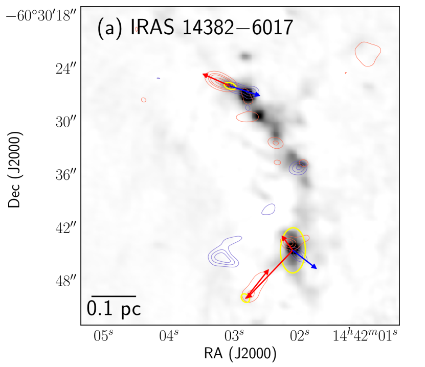
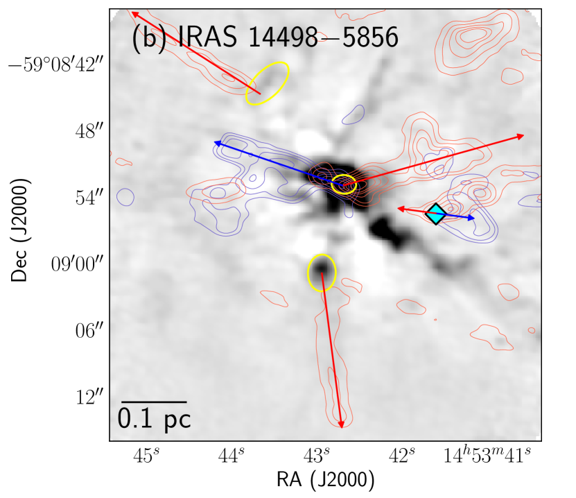
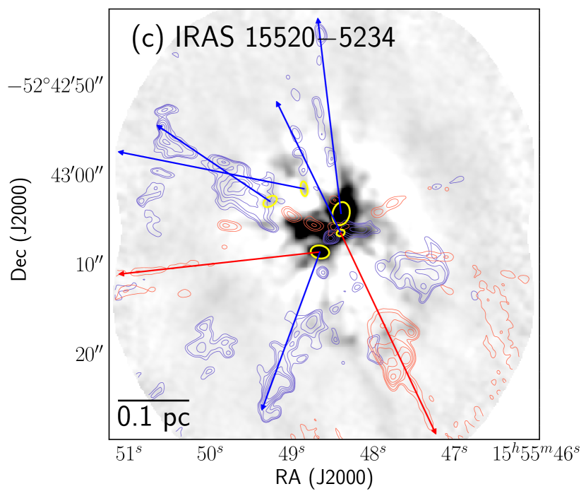
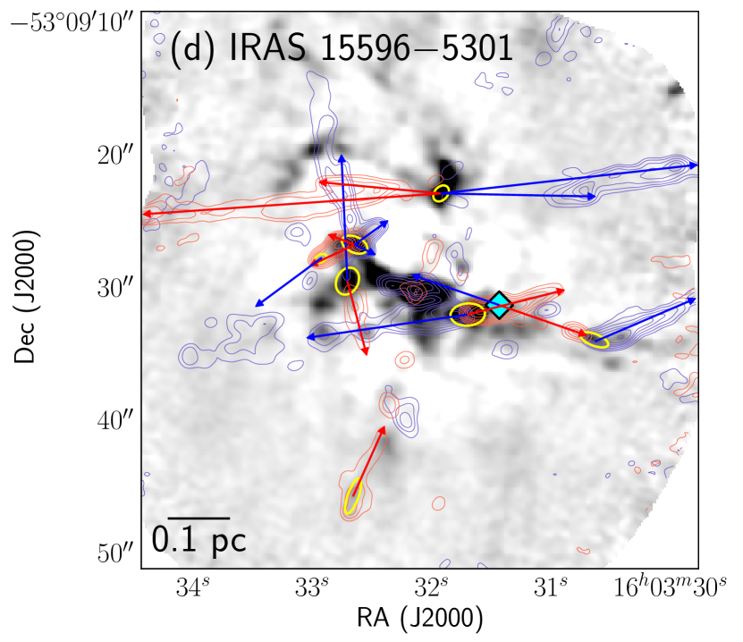
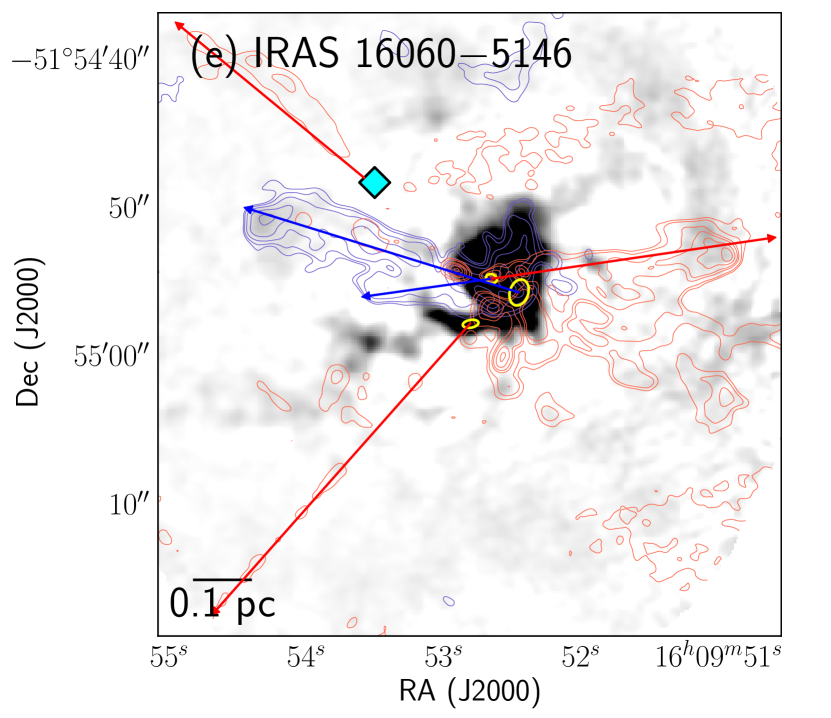
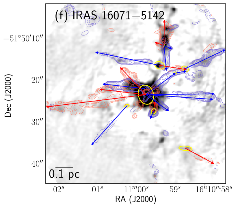
Figure 1.— Images of molecular outflows in the first six target fields listed in Table 1. Background grey-scale images are the ALMA 0.9 mm continuum maps. The red and blue contours correspond to red and blue-shifted CO(3–2) gas integrated over carefully selected velocity ranges to depict the outflow lobes. The blue and red outflow lobes are also marked by blue and red arrows, respectively. The driving sources as shown by continuum emission are marked in yellow ellipses. Outflow lobes with cyan diamonds are those for which no continuum sources are identified.

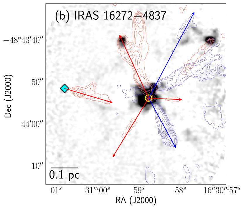
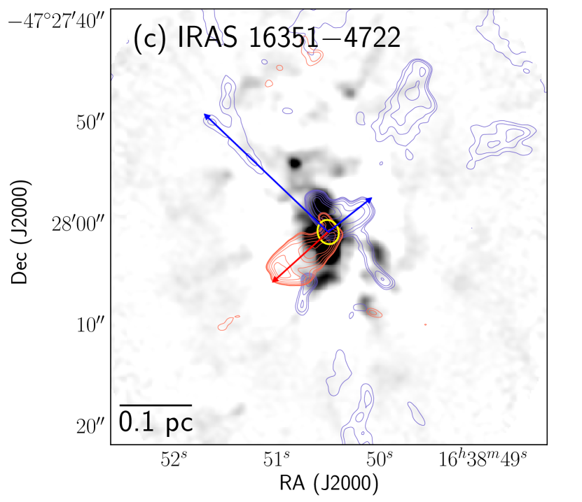
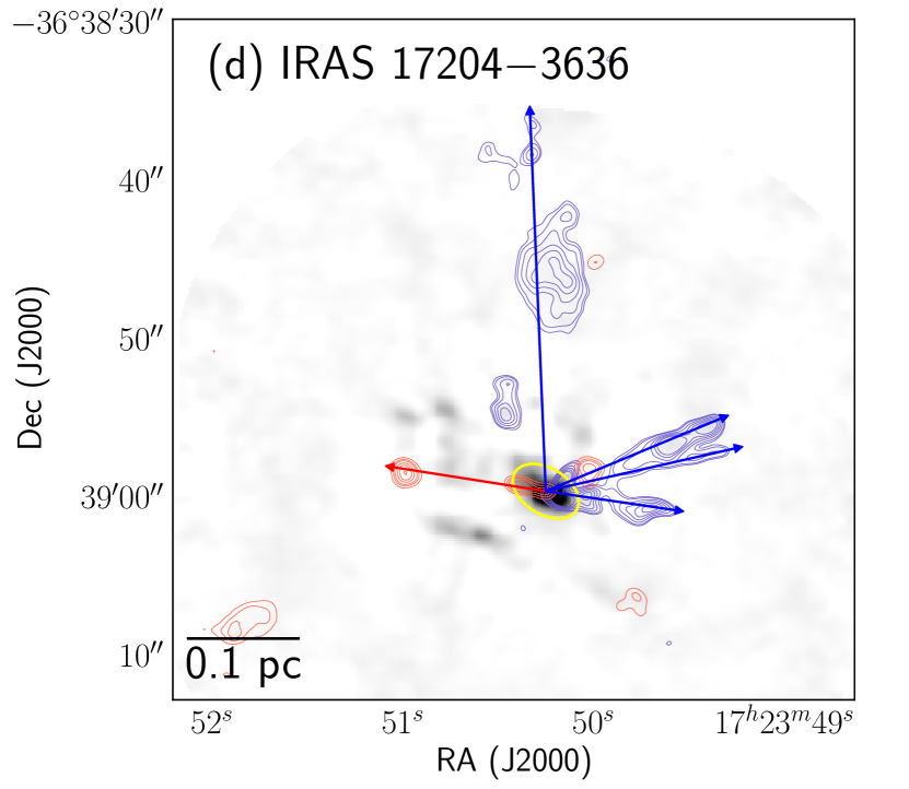
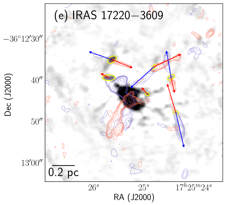
Figure 1 (Cont.).— Images of molecular outflows for the last five target fields listed in Table 1. The symbols are the same as in Figure 1.

After completing the preliminary identification of outflows in the averaged small data cubes, we finally inspected the original data cubes for the same set of outflows to obtain their final parameters. This also helped us to identify lower velocity outflows that were not detected in the integrated channel maps. In addition, other outflow tracers of outflows (e.g., HCN, SiO) were used to confirm a few confusing outflow lobes. The peak velocity and extent of each outflow were considered up to a 5$\sigma$ level where $\sigma$ is the rms measured from a few line-free channels. Details of all identified outflows such as the coordinates of the continuum sources, assigned names, orientations of outflow lobes in the plane of sky, orientation of lobes with respect to underlying filaments, magnetic field orientation and Galactic plane (see following sections), peak velocity, and extent of each outflow are presented in Table 2. For five outflow lobes, no continuum sources were detected as they are possibly below our detection limit. The outflow lobes overlaid on the 0.9 mm ALMA continuum maps for all the regions are presented in Figure 1. We finally identified a total of hundred and five outflow lobes. Among them 32 are bipolar and 41 are unipolar in nature.

3.2. Identification of host clouds and filaments

The primary aim of our study is to examine whether the orientation of outflow lobes have a dependence on large-scale filamentary accretion and also with the orientation of the magnetic fields or Galactic plane. Thus, we examined integrated ThrUMMS ¹³CO maps and the ATLASGAL dust continuum maps to identify the host clouds and large-scale filamentary structures. To generate the integrated intensity maps, velocity ranges of all the clouds were determined from the ¹³CO spectrum along the direction of each target. Priority is given to the clouds structures traced in ThrUMMS ¹³CO data over the ATLASGAL images as the integrated ¹³CO data for a specific velocity range suffers from least contamination from the foreground and background emission compared to ATLASGAL maps. However, ¹³CO data were not available for IRAS 17204-3636 and IRAS 17220-3609 regions. Thus, for these two regions, we identified clouds based on the 870 $\mu m$ ATLASGAL image.

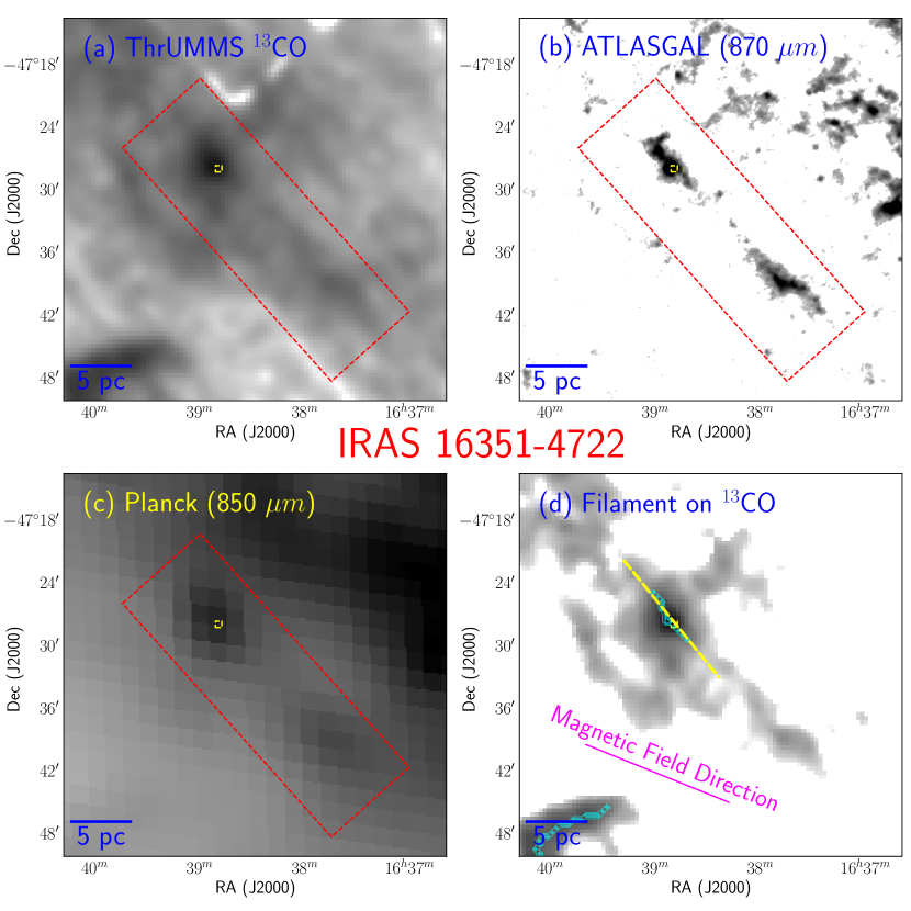
Figure 2.— Distribution of gas and dust in the IRAS 16351-4722 region. (a) Velocity integrated ThrUMMS ¹³CO map of the large 21${}^{\prime}\times$21^′ area around IRAS 16351-4722. The field of view of ALMA observations is shown by a small yellow box toward the center. The red rectangle shows the extent of the cloud.(b) ATLASGAL 870 $\mu m$ dust image of the same area. (c) Planck 850 $\mu m$ image of the same area. (d) Filaments marked on the ThrUMMS ¹³CO map. The filament skeletons are also shown by cyan contours. Large-scale orientation of the filament is shown by an eye-fitted yellow dashed line. Position angle of the magnetic field is also shown by a magenta line. Magnetic field PA is estimated by averaging the polarization position angles of the Planck 850 $\mu m$ dust polarization map within the dashed red rectangle shown in other panels.

Python-based filfinder algorithm (Koch & Rosolowsky, 2015) was applied on all the identified molecular clouds to trace the filamentary structures. filfinder is capable of finding filaments even with low surface brightness as the algorithm uses an arctangent transform on the image. This algorithm identify all the possible filamentary structures across the input map followed by a method to determine their skeletons via the Medial Axis Transform. To identify the filaments, we ran the filfinder algorithm with inputs like the global background thresholds and thresholds for length of skeletons. Note that the primary beam of our ALMA data (36^′′) is comparable or even smaller than the angular resolution of the ATLASGAL (19$\farcs$2) and ThrUMMS ¹³CO data (66^′′) making it difficult to determine the filament orientation at the scale of ALMA field of view (PA_Fil). So, we only considered the large scale PAs of filaments estimated by a visual fit over the large-scale filfinder skeletons. By large-scale PAs, we imply the average PAs over at least 5 pixels of the identified skeleton (i.e., $\sim$3–4 pc at the distances of our targets). Note that a visual fit to filaments might not be as accurate as a statistical fit. However, visual fits to these large-scale PA_Fil have typical uncertainty $\lesssim$10$\arcdeg$. We also considered elongated clumps (aspect ratio $<$ 5) as filamentary structure because such structures may also aid in gas-flow along a preferred direction like filaments.

Filaments are detected toward 7 targets, and corresponding PA_Fil are listed in Table 1. The remaining four targets are associated with round-shaped clumps that have no preferred orientations. The distribution of integrated ¹³CO and dust emission toward two representative regions, one with filaments (IRAS 16351-4722) and another without filaments (IRAS 15520-5234) are shown in Figures 2 and 3. The extents of the identified clouds are also marked in both figures. We have also shown the Planck 850 $\mu m$ dust emission as Planck data is used to determine the magnetic field PAs in our study (following section). The filament mask identified by the filfinder algorithm, and a visual fit to the filament is also shown in Figure 2d. Figures corresponding to the remaining targets are presented in Appendix A.

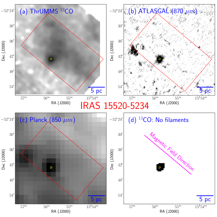
Figure 3.— Distribution of gas and dust in the IRAS 15520-5234 region where no filamentary structure is detected in the integrated ¹³CO and ATLASGAL 870 $\mu m$ images. Symbols are the same as in Figure 2.

3.3. Magnetic field position angle

Our purpose of using Planck polarization data is to infer the mean orientation of magnetic field around our targets as magnetic field also often aid in star formation. We estimated the mean linear polarization PAs over the cloud extent identified in the previous section. The conventional relation for PAs, $\theta_{\mathrm{GAL}}=0.5\,\times\,arctan(U,Q)$ (where, arctan avoids the $\pi$ ambiguity) yields PAs in Galactic coordinates in the range $-90\arcdeg<\theta<+90\arcdeg$, where $\theta_{\mathrm{GAL}}$ $=$ 0$\arcdeg$ pointing towards the Galactic North but increasing towards Galactic West. But in order to follow the IAU convention (i.e., $\theta_{\mathrm{GAL}}$ $=$ 0$\arcdeg$ points Galactic North but increases toward Galactic East), the $\theta_{\mathrm{GAL}}$ values were derived by using the relation

$$\theta_{\mathrm{GAL}}=0.5\,\times\,arctan(-U,Q).$$ (1)

The magnetic field orientations in Galactic coordinates can be obtained by adding 90$\arcdeg$ to $\theta_{\mathrm{GAL}}$, i.e., $\theta^{\prime}_{B}$ = 90$\arcdeg$ + $\theta_{\mathrm{GAL}}$ (for details see Planck Collaboration et al., 2016c, d, and references therein).

Furthermore, the magnetic field orientation in celestial coordinates (FK5, J2000) is obtained using the following relation given in Corradi et al. (1998)

$$\psi=arctan\left[\frac{cos(l-32.9\arcdeg)}{cos\,b~{}cot\,62.9\arcdeg~{}-~{}sin\,b~{}sin(l-32.9\arcdeg)}\right],$$ (2)

where $\psi$ is the angle subtended at the position of each object by the direction of the equatorial North and the Galactic North. The $l$ and $b$ are the Galactic coordinates of each pixel with a polarization measurement. We then transform the magnetic field orientations from Galactic ($\theta^{\prime}_{B}$) to equatorial ($\theta_{B}$) coordinate system using the relation

$$\theta_{B}={\theta^{\prime}_{B}}-\psi$$ (3)

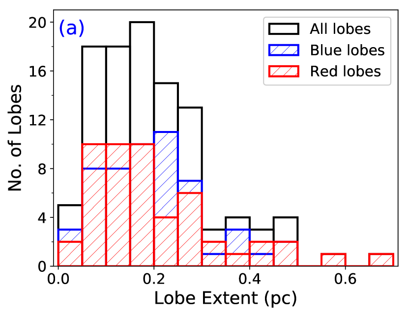
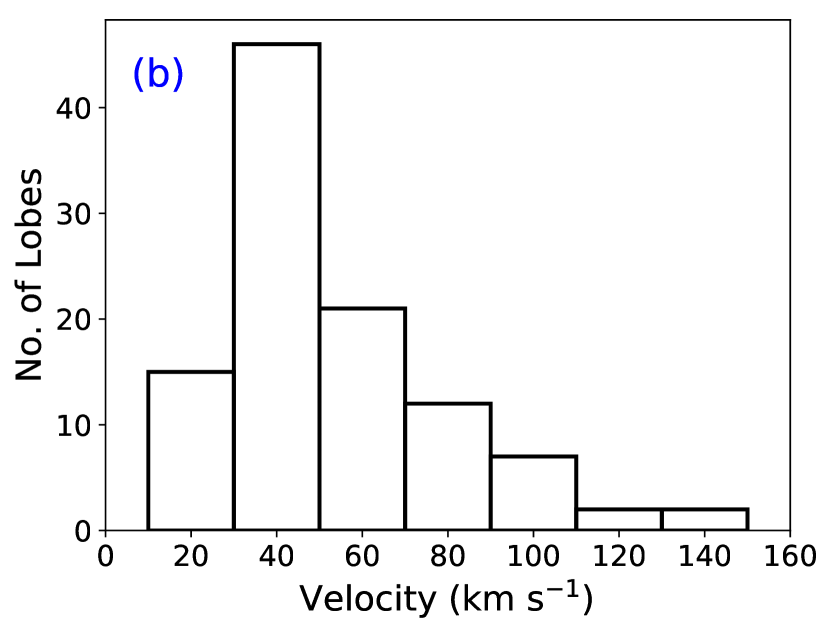
Figure 4.— (a) Stacked histogram of extents of all the identified outflows. Extents for blue and red-lobes are also shown as blue and red histograms. (b) Histogram of the peak velocities of all the identified outflows.

Finally, we have estimated the mean magnetic field orientation using the $\theta_{B}$ vectors distributed within the area of the clouds identified in the previous section. The mean values of $\theta_{B}$ and the corresponding standard deviations are listed in Table 1. The mean magnetic field direction toward IRAS 14498-5856 and IRAS 15520-5234 regions are also marked in Figures 2d and 3d.

3.4. Statistics of Outflow extent and Velocities

We have measured the projected plane of sky extent and maximum red-blue velocities of all identified outflow lobes. The plane of sky extent of outflow lobes are converted into physical scale (in pc) using the distances listed in Table 1. A histogram for all the measured outflow extents are presented in Figure 4a, along with the histograms for extents of red and blue lobes separately. Red and blue lobes typically show a similar shape signify an unbiased identification of the outflow lobes. Sky projected extent of outflows lobes have a range of 0.05–0.7 pc peaking at around 0.2 pc. Similarly, we constructed a histogram for peak outflow velocities which is presented in Figure 4b. Most of outflows have plane of sky projected velocities below 50 km s^-1. However, a few outflows are seen with significantly higher velocities (up to 150 km s^-1), and also a few among them have extended outflow lobes more than 0.2 pc. With an average outflow extent of 0.2 pc and peak outflow velocity of 40 km s^-1, the typical dynamical time-scale is about 5$\times$10³ yr. The average mass of the driving continuum sources is 15 M_⊙ (with T${}_{\mathrm{dust}}\sim$ 20 K and spectral index, $\beta~{}\sim$2.0) and have typical outflowing mass of 0.5 M_⊙ (details are not presented in this paper). Such extended massive outflow lobes can be results of energetic driving protostars. Understanding of this scenario demands a detailed analysis of gas dynamics and momentum budget of the outflows, which will be presented in a forthcoming paper.

3.5. Outflow Position Angles

The PAs of all outflow lobes (PA_lobe) were measured from the celestial North pole. The PAs for both blue and red-shifted lobes are measured independently. We are only interested in the the orientations of the lobes, and hence, alloted them with values in the range from -90$\arcdeg$ to +90$\arcdeg$ counterclockwise from the celestial North (see Table 2). Thus, the PAs in first quadrant have negative signs, and PAs in the second quadrant have positive signs.

We constructed histograms of the absolute values of the measured PA_lobe (ignoring the signs) considering each lobe as independent (Figure 5). Histograms are constructed separately for the outflows associated with the filaments and with round-shaped/circular clumps. The outflows associated with circular clumps can be treated as a control region as they do not have any preferred direction of gas accretion like filaments. Although, the overall distribution of PA_lobe has a rising trend at $\sim$90$\arcdeg$, lobes associated with filaments do not have any preferred plane of sky direction (Figure 5a). The distribution is skewed toward PA${}_{\mathrm{lobe}}~{}=$ 90$\arcdeg$ as the outflow lobes associated with the circular clumps mostly oriented at PA_lobe in the range from 50–90$\arcdeg$.

3.5.1 PA_lobe with respect to magnetic field and Galactic plane

As mentioned before, magnetic field plays important roles at different evolutionary phases and spatial scales of star formation. Hence, in this study, we also searched for any correlation of the PA_lobe with respect to the large-scale magnetic field orientation. We measured the projected plane of sky angles between PAs of large-scale magnetic field (see $\theta_{B}$ values in Table 1) and PA_lobe (hereafter $\gamma_{B}$). The following equation was used to estimate the $\gamma_{B}$ values,

$$\gamma_{B}=\mathrm{MIN}\{|\mathrm{PA}_{\mathrm{lobe}}-\theta_{B}|,|\mathrm{PA}_{\mathrm{lobe}}-\theta_{B}|-90\arcdeg\},$$ (4)

where $\gamma_{B}$ has ranges between 0^∘ and 90^∘.

Note that previous studies on Galactic large-scale filaments showed most of them generally aligned with the Galactic plane (Wang et al., 2015, 2016) Thus, it might be important to also examine the projected plane of sky angles between PAs of Galactic plane (i.e., PA_GP; see Table 1) and PA_lobe (hereafter $\gamma_{\mathrm{GP}}$). The $\gamma_{\mathrm{GP}}$ values are calculated in similar convention as mentioned in Eq 4.

Histograms for both $\gamma_{B}$ and $\gamma_{\mathrm{GP}}$ are shown in Figure 5b. No specific trend in the distributions is noted in both the cases. This particular result indicates toward a non-correlation of the outflow axes with the large-scale magnetic field orientation as well as with the Galactic plane.

3.5.2 Orientation of Outflows and Filaments

Our primary interest in this paper is to search for the presence of any preferred angle of outflows with respect to their host filaments. Filamentary structures are seen in 7 regions (see Section 3.2). These 7 targets contain a total of 49 outflow lobes. The PA_Fil values of the identified filaments are listed in Table 1.

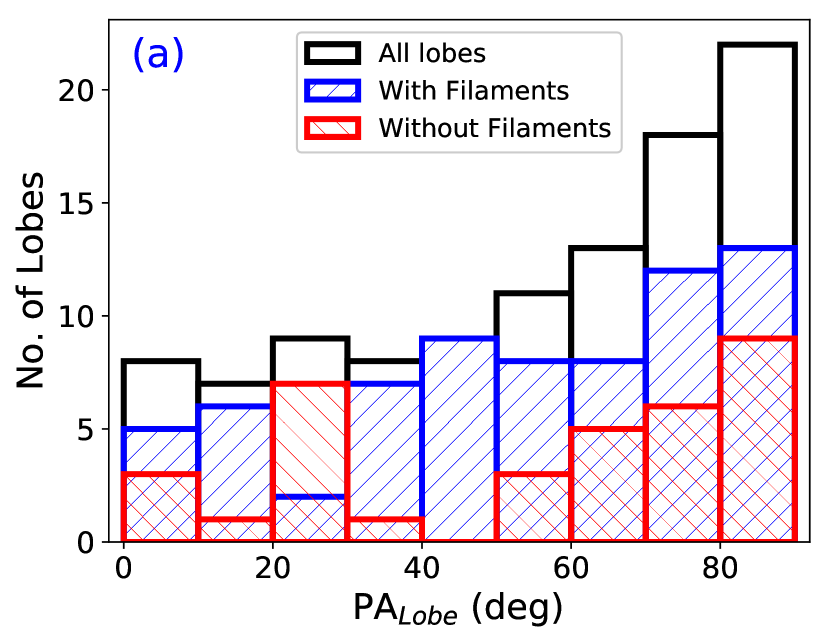
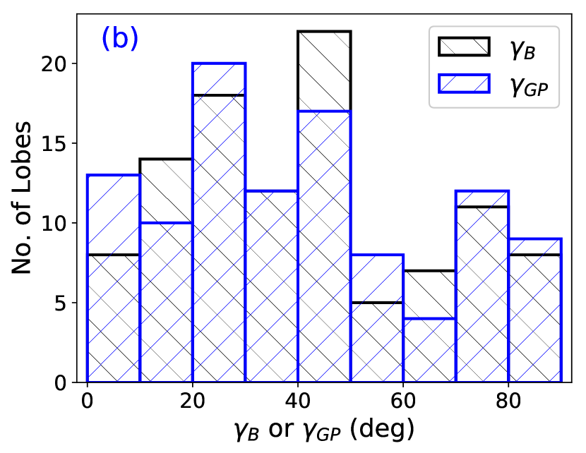
Figure 5.— (a) Stacked histogram of PAs of all the identified outflow lobes associated with filaments and circular clumps. (b) Stacked histograms of projected separations of PAs of all the lobes with respect to magnetic field orientation ($\gamma_{B}$) and Galactic plane ($\gamma_{GP}$).

We further measured the projected PAs between PA_lobe and PA_Fil (i.e., $\gamma_{\mathrm{Fil}}$) for all the lobes in these 7 regions following the same convention used in Eq 4. In Figure 6a, we present the histogram of all the $\gamma_{Fil}$. In addition, histogram of $\gamma_{\mathrm{Fil}}$ for those particular lobes for which the host filaments are oriented along the magnetic field (namely, IRAS 14382-6017, IRAS 14498-5856, IRAS 16071-5142, and IRAS 16076-5134) is also presented in Figure 6a. No specific trend is apparent in the histograms, except both the histograms are slightly devoid of outflow lobes at $\gamma_{\mathrm{Fil}}\sim$60$\arcdeg$. We further constructed a cumulative histogram of $\gamma_{\mathrm{Fil}}$ (Figure 6b). It is apparent in the cumulative histogram that $\gamma_{\mathrm{Fil}}$ for all 7 regions with filaments, and also filaments aligned with magnetic fields do not show any specific trend. In fact, the distribution seems to be random in nature, and follow closely the random distribution curve shown in Figure 6b.

Note that we measured PAs of outflow lobes and filaments on the plane of sky. The measured $\gamma_{\mathrm{Fil}}$ value is thus a plane of sky projection of the actual three-dimensional angle between outflow axes and their host filament ($\gamma_{\mathrm{3D}}$). Hence, the observed $\gamma_{\mathrm{Fil}}$ values might appear with a different distribution than the original distribution of $\gamma_{\mathrm{3D}}$ (see detailed discussions by Stephens et al., 2017). To examine the projection effect on the measured $\gamma_{\mathrm{Fil}}$ distribution, we carried out a Monte Carlo simulation. The detailed methodology can be found in Stephens et al. (2017). In brief, we randomly generated 2$\times$10⁶ radially outward pairs of unit vectors on the surface of a sphere. Then we calculated the real 3D PA between the two unit vectors ($\gamma_{\mathrm{3D}}$), and also their 2D PA ($\gamma_{\mathrm{2D}}$) assuming they are projected onto the y-z plane. These $\gamma_{\mathrm{2D}}$ values are equivalent to the observed $\gamma_{\mathrm{Fil}}$. Finally, we calculated the cumulative distribution function (CDF) of $\gamma_{\mathrm{2D}}$ considering three scenarios of $\gamma_{\mathrm{3D}}$ values: (1) parallel where $\gamma_{\mathrm{3D}}$ ranging from 0$\arcdeg$ to 20$\arcdeg$, (2) perpendicular where $\gamma_{\mathrm{3D}}$ ranging from 70$\arcdeg$ to 90$\arcdeg$, and (3) random where $\gamma_{\mathrm{3D}}$ ranging from 0$\arcdeg$ to 90$\arcdeg$. These simulated CDFs are also shown in Figure 6b. Although, our observed CDF of $\gamma_{\mathrm{Fil}}$ typically follow the random distribution, it also deviates slightly. We thus tried a combined CDF for random and $\gamma_{3D}$ values from 10$\arcdeg$ to 40$\arcdeg$ that may better represent the observed CDF of $\gamma_{\mathrm{Fil}}$. Accordingly, we found that the observed distribution $\gamma_{\mathrm{Fil}}$ can be reproduced if additional 10% sources in a random distribution have preferred $\gamma_{\mathrm{3D}}$ values from 10$\arcdeg$ to 40$\arcdeg$. Note that the uncertainties in the measured PAs are about $\sim$10$\arcdeg$. Thus, the simulated CDF with 10% more sources in preferred direction from 10$\arcdeg$–40$\arcdeg$ which better represents the observed $\gamma_{\mathrm{Fil}}$ CDF might not be significant.

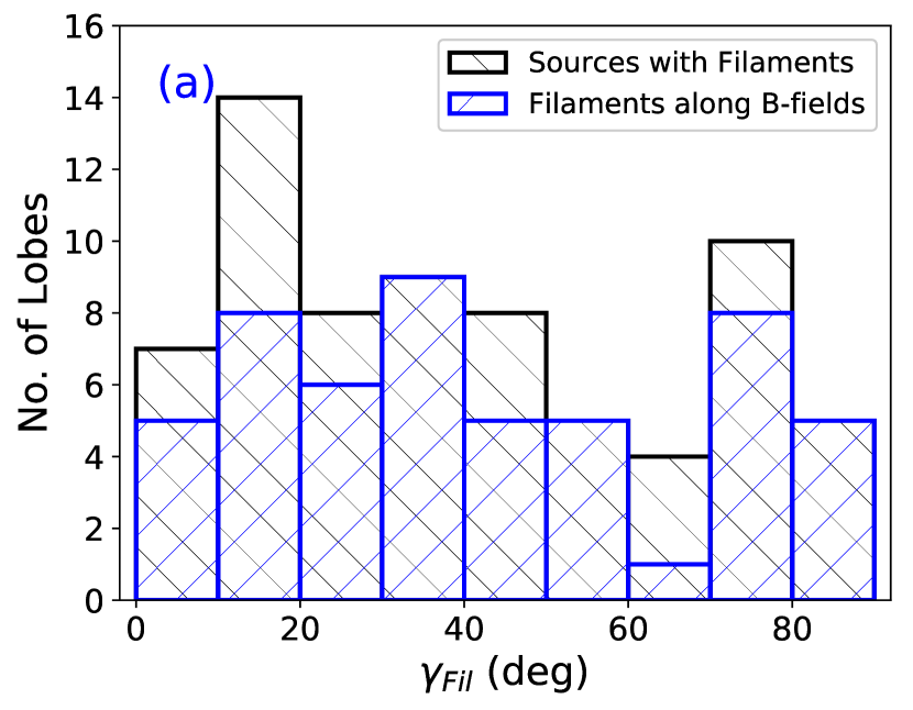
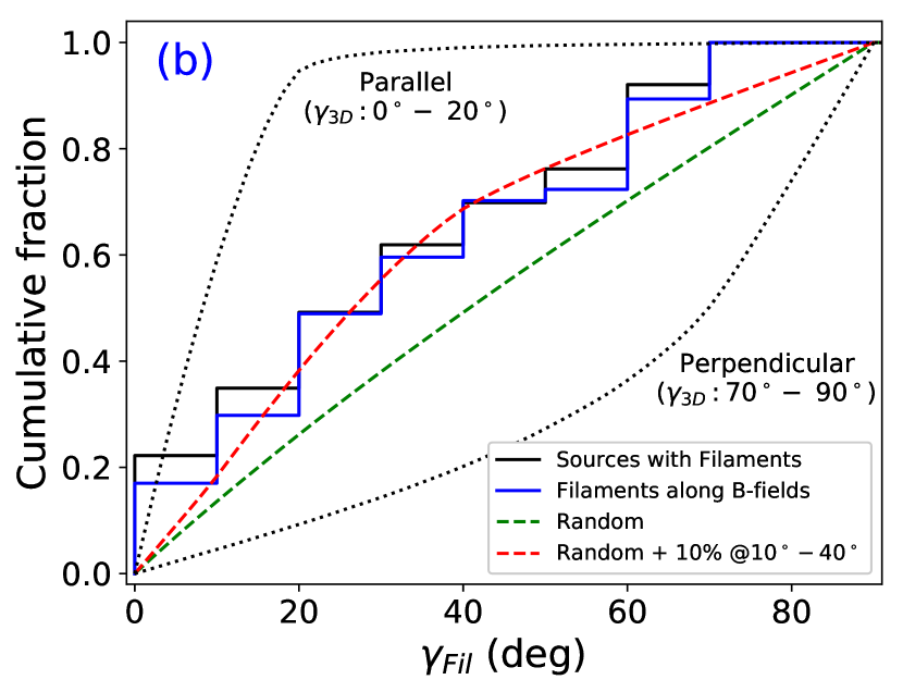
Figure 6.— (a) Histogram of $\gamma_{\mathrm{Fil}}$ (i.e., the angle between the PA_Out and PA_Fil). (b) Cumulative distribution function of $\gamma_{\mathrm{Fil}}$. Green line shows the CDF of randomly distributed $\gamma_{\mathrm{3D}}$ values. Two black dotted lines show parallel and perpendicular distributions of $\gamma_{3D}$ values. Red line represent the CDF for the randomly distributed $\gamma_{\mathrm{3D}}$ values with additional 10% sources that are oriented along 10$\arcdeg$–40$\arcdeg$. The red line better represents the observed CDF of $\gamma_{\mathrm{Fil}}$.

Table 2Outflow parameters

Continuum Source		Outflow	PAlobe (∘)		$\gamma_{\mathrm{Fil}}$ (∘)		$\gamma_{B}$ (∘)		$\gamma_{\mathrm{GP}}$ (∘)		$v_{\mathrm{peak}}$ (km s-1)		Extent (pc)
RA (J2000)	Dec (J2000)	Name	Red	Blue	Red	Blue	Red	Blue	Red	Blue	Red	Blue	Red	Blue
14 42 02.106	-60 30 44.59	I14382_o1a	37	52	-28	-13	-34	-19	-29	-14	49.5	46.7	0.041	0.067
		I14382_o1b	-38	–	77	–	71	–	76	–	55.6	–	0.148	–
14 42 03.066	-60 30 26.02	I14382_o2	66	72	1	7	-5	1	0	6	70.4	72.7	0.067	0.070
14 42 02.833	-60 30 49.99	I14382_o3	-38	–	77	–	71	–	76	–	31.3	–	0.083	–
14 53 42.681	-59 08 52.88	I14498_o1a	-74	–	73	–	45	–	43	–	119.0	–	0.263	–
		I14498_o1b	–	71	–	38	–	10	–	8	–	65.6	–	0.190
$\ast\ast$	$\ast\ast$	I14498_o2	82	83	49	50	21	22	19	20	65.3	69.1	0.054	0.054
14 53 43.579	-59 08 43.78	I14498_o3	57	–	24	–	-4	–	-6	–	19.3	–	0.213	–
14 53 42.941	-59 09 00.87	I14498_o4	6	–	-27	–	-55	–	-57	–	25.4	–	0.151	–
15 55 48.398	-52 43 06.53	I15520_o1	25	26	–	–	-25	-24	-25	-24	28.1	32.6	0.313	0.206
15 55 48.654	-52 43 08.66	I15520_o2a	-84	–	–	–	46	–	46	–	42.0	–	0.284	–
		I15520_o2b	–	-20	–	–	–	-70	–	-70	–	32.6	–	0.236
15 55 48.393	-52 43 04.38	I15520_o3	–	7	–	–	–	-43	–	-43	–	23.9	–	0.276
15 55 48.848	-52 43 01.61	I15520_o4	–	79	–	–	–	29	–	29	–	61.2	–	0.266
15 55 49.265	-52 43 03.02	I15520_o5	–	56	–	–	–	6	–	6	–	68.1	–	0.191
16 03 31.921	-53 09 22.96	I15596_o1a	-86	-84	–	–	44	46	45	47	41.7	48.4	0.480	0.415
		I15596_o1b	85	89	–	–	35	39	36	40	33.1	54.5	0.196	0.248
16 03 32.646	-53 09 26.82	I15596_o2a	-65	-54	–	–	65	76	66	77	88.5	51.0	0.079	0.066
		I15596_o2b	69	64	–	–	19	14	20	15	72.9	84.9	0.045	0.037
16 03 32.656	-53 09 45.76	I15596_o3	-24	–	–	–	-74	–	-73	–	55.6	–	0.123	–
16 03 32.705	-53 09 29.57	I15596_o4	15	3	–	–	-35	-47	-34	-46	49.5	42.4	0.123	0.203
16 03 31.697	-53 09 32.09	I15596_o5	-76	-82	–	–	54	48	55	49	104.1	95.3	0.160	0.261
$\ast\ast$	$\ast\ast$	I15596_o6	71	71	–	–	21	21	22	22	72.1	51.0	0.148	0.148
16 03 32.927	-53 09 27.85	I15596_o7	–	-53	–	–	–	77	–	78	–	33.7	–	0.130
16 03 30.635	-53 09 33.99	I15596_o8	–	-68	–	–	–	62	–	63	–	82.3	–	0.175
16 09 52.650	-51 54 54.86	I16060_o1	-82	-82	-22	-22	48	48	51	51	40.1	34.5	0.488	0.223
16 09 52.450	-51 54 55.79	I16060_o2	–	73	–	-47	–	23	–	26	–	50.1	–	0.488
$\ast\ast$	$\ast\ast$	I16060_o3	50	–	-70	–	0	–	3	–	39.2	–	0.416	–
16 09 52.803	-51 54 57.90	I16060_o4	-42	–	18	–	88	–	-89	–	26.2	–	0.662	–
16 10 59.750	-51 50 23.54	I16071_o1a	-83	-89	44	38	56	50	50	44	70.2	56.3	0.571	0.387
		I16071_o1b	83	86	30	33	42	45	36	39	31.2	35.5	0.264	0.380
		I16071_o1c	43	54	-10	1	2	13	-4	7	52.9	39.9	0.213	0.158
		I16071_o1d	–	84	–	31	–	43	–	37	–	142.2	–	0.240
		I16071_o1e	–	-75	–	52	–	64	–	58	–	90.1	–	0.465
16 10 59.553	-51 50 27.51	I16071_o2	-7	-23	-60	-76	-48	-64	-54	-70	148.3	109.2	0.054	0.045
16 10 59.400	-51 50 16.52	I16071_o3	78	81	25	28	37	40	31	34	31.2	28.6	0.371	0.154
16 11 00.242	-51 50 26.22	I16071_o4	–	-42	–	85	–	-83	–	-89	–	19.1	–	0.299
16 10 58.732	-51 50 36.37	I16071_o5	62	–	9	–	21	–	15	–	31.2	–	0.183	–
16 10 59.286	-51 50 11.78	I16071_o6	71	67	18	14	30	26	24	20	33.8	94.5	0.054	0.047
16 10 59.286	-51 50 11.78	I16071_o7	-1	6	-54	-47	-42	-35	-48	-41	87.6	65.9	0.145	0.142
16 11 26.540	-51 41 57.32	I16076_o1a	51	47	14	10	4	0	4	0	85.2	41.4	0.136	0.080
		I16076_o1b	18	20	-19	-17	-29	-27	-29	-27	111.2	27.5	0.144	0.120
		I16076_o1c	-59	–	84	–	74	–	74	–	68.7	–	0.162	–
		I16076_o1d	76	64	39	27	29	17	29	17	80.9	87.3	0.066	0.107
		I16076_o1e	-62	–	81	–	71	–	71	–	35.8	–	0.184	–
		I16076_o1f	-45	–	-82	–	88	–	88	–	35.8	–	0.216	–
		I16076_o1g	71	72	34	35	24	25	24	25	35.8	63.1	0.205	0.098
		I16076_o1h	-50	-71	-87	72	83	62	83	62	32.3	31.0	0.170	0.203
		I16076_o1i	–	6	–	-31	–	-41	–	-41	–	56.1	–	0.194
		I16076_o1j	–	30	–	-7	–	-17	–	-17	–	32.7	–	0.166
		I16076_o1k	–	-35	–	-72	–	-82	–	-82	–	52.7	–	0.108
		I16076_o1l	–	-37	–	-74	–	-84	–	-84	–	35.3	–	0.128
16 11 27.384	-51 41 50.21	I16076_o2	-12	–	-49	–	-59	–	-59	–	35.8	–	0.412	–
16 11 27.697	-51 41 55.36	I16076_o3	–	-36	–	-73	–	-83	–	-83	–	36.2	–	0.299
16 11 26.876	-51 41 55.92	I16076_o4	-89	–	54	–	44	–	44	–	36.6	–	0.155	–
16 11 26.876	-51 41 55.92	I16076_o5	–	-88	–	55	–	45	–	45	–	37.9	–	0.076
$\ast\ast$	$\ast\ast$	I16076_o6	–	84	–	47	–	37	–	37	–	23.2	–	0.167
16 30 58.770	-48 43 53.89	I16272_o1a	25	29	–	–	-16	-12	-18	-14	68.0	41.2	0.256	0.209
		I16272_o1b	-31	-28	–	–	-72	-69	-74	-71	22.9	20.4	0.254	0.359
		I16272_o1c	87	–	–	–	46	–	44	–	31.6	–	0.122	–
$\ast\ast$	$\ast\ast$	I16272_o2	74	–	–	–	33	–	31	–	47.2	–	0.184	–
16 38 50.501	-47 28 00.91	I16351_o1a	58	41	19	2	-10	-27	16	-1	92.0	21.6	0.090	0.092
		I16351_o1b	–	46	–	7	–	-22	–	4	–	35.4	–	0.237
17 23 50.249	-36 38 59.66	I17204_o1a	81	82	–	–	45	46	47	48	20.2	40.5	0.144	0.123
		I17204_o1b	–	-77	–	–	–	67	–	69	–	32.7	–	0.179
		I17204_o1c	–	-67	–	–	–	77	–	79	–	35.3	–	0.175
		I17204_o1d	–	2	–	–	–	-34	–	-32	–	24.9	–	0.342
17 25 25.635	-36 12 35.12	I17220_o1	68	71	68	71	38	41	34	37	28.4	32.3	0.196	0.215
17 25 24.796	-36 12 36.85	I17220_o2	-65	-48	-65	-48	85	-78	81	-82	97.8	49.6	0.265	0.280
17 25 24.357	-36 12 47.89	I17220_o3	13	17	13	17	-17	-13	-21	-17	35.4	55.7	0.316	0.264
17 25 24.453	-36 12 39.36	I17220_o4	13	10	13	10	-17	-20	-21	-24	33.6	52.2	0.140	0.238
17 25 24.926	-36 12 43.44	I17220_o5	41	–	41	–	11	–	7	–	30.2	–	0.076	–
17 25 25.697	-36 12 39.48	I17220_o6	62	–	62	–	32	–	28	–	34.5	–	0.080	–

4. Discussion

The projected momentum axes of outflow lobes in our studied protoclusters do not show any preferred direction with respect to the observed filaments. The $\gamma_{\mathrm{Fil}}$ are in fact distributed in a random fashion (see Figure 6b). For further confirmation of the randomness, we performed a statistical Kolmogorov–Smirnov (K–S) test on the observed CDF of $\gamma_{\mathrm{Fil}}$ with the simulated CDFs for random and random$+$preferred(10% in 10$\arcdeg$–40$\arcdeg$) $\gamma_{\mathrm{3D}}$ values. Both the tests produce $p-$values more than 0.8 which imply that we cannot reject the null hypothesis at a level of 80% or lower. This particular test indicates that the distribution is likely to be random in nature (with at least 80% confidence). In addition, our identified outflow lobes do not show any preferred orientation with respect to the large-scale magnetic field as well as with the Galactic plane.

Random orientation of outflow lobes on the plane of sky for every origin indeed refers that the distribution of $\gamma_{\mathrm{Fil}}$ is really random in nature. Note that we identified filaments with a visual fit to the filfinder skeletons, and the uncertainties in the large-scale PA_Fil are typically $\lesssim$10$\arcdeg$. Thus, we also constructed cumulative distribution of $\gamma_{\mathrm{Fil}}$ values by adding a random number in range of $\pm$10$\arcdeg$. The cumulative distribution does not show any significant change compared to the original curve. Two such examples are shown in Figure 9 (Cont.) in Appendix B. Thus, a robust identification of filaments may only slightly improve the statistics but not the overall finding of this study.

Filamentary structures in molecular clouds may develop through several physical processes, and accretion through filaments also vary depending on the presence of the magnetic fields (see Stephens et al., 2017, for more detailed discussion). Observational studies of Hacar et al. (2013) and Pineda et al. (2011) suggest that filaments may fragment into smaller substructures, which may significantly affect the initial conditions for protostellar accretion and collapse. These prolate shaped substructures are generally aligned along the filaments (Pineda et al., 2011; Hacar et al., 2013), but this is not the case always (Pineda et al., 2015). Formation of protostars within these arbitrarily distributed smaller substructures may thus lead to a random direction of outflows.

Magnetic fields are known to play a crucial role in both low- and high-mass star formation (Hull & Zhang, 2019) but only at tens of pc to sub-pc scales (Li et al., 2013; Zhang et al., 2014; Santos et al., 2016). The role of the magnetic field becomes less important compared to gravity and angular momentum at the core to disk scale (0.01 pc; Zhang et al., 2014). In a study of low-mass star-forming cores, Hull et al. (2014) found no correlation between outflow axis and envelope magnetic fields. Simulation of Li, P.-S. et al. (2015) showed that the local small scale (i.e., clump/core scale) magnetic field and filament orientations can be substantially different from the large scale orientations. The deviation in orientation also depends on the gas density of the cores and filaments. Even if the local magnetic field aligned with the large scale magnetic field, the turbulence within cores may lead to misalignment of outflow axes and magnetic field (Gray et al., 2018). With Planck polarization data, we could only estimate the large-scale (a few pc) magnetic field which was compared with the sub-pc scale driving sources. The internal dynamics and magnetic field at core-scale could be highly different from that measured in the large-scale. This could be a possible reason of non-correlation of $\theta_{B}$ with PA_lobe.

Earlier, Davis et al. (2009) and Stephens et al. (2017) also found a random alignment of molecular outflows (i.e., momentum axes) with respect to the filament/core directions in nearby Galactic star-forming regions. In contrast, Anathpindika & Whitworth (2008), Wang et al. (2011), and Kong et al. (2019) found that the momentum axes of outflows are preferentially oriented perpendicular to the filaments. Numerical simulations suggest both scenarios are possible depending upon the initial condition of the host cloud that formed the filaments, on their surrounding environment, and the presence of magnetic fields. In fact, momentum axes of outflows may vary significantly depending on how exactly the accretion occurs to the central protostars. For example, on the one hand, Clarke et al. (2017) showed that accretion onto a filament occurring from a turbulent environment may produce vorticity which have angular momentum parallel to the axis of the filament.

On the other hand, magnetic fields also play a crucial role in star formation (Machida et al., 2005, 2019; Hull & Zhang, 2019). Simulations show that orientation of outflows with respect to their parent cores (thus, the filaments) could depend strongly on the relative strengths of the magnetic field, turbulence, and rotation (Machida et al., 2005; Offner et al., 2016; Lee et al., 2017). It is important to note that although the feedback from star formation is energetically important (Arce et al., 2011) and is capable of sustaining turbulence even in a low mass star forming region (Li, H. et al., 2015), the dynamic flow seems to de-couple from filament in the protostellar accretion phase based on the results here. Recently, Li & Klein (2019) suggested for a possibility of perpendicular alignment of momentum axis in the moderately strong magnetized filaments. While some observations revealed magnetic field lines to be perpendicular to the orientation of the filament (see e.g., Matthews, & Wilson, 2000; Santos et al., 2016), Galametz et al. (2018) showed a bimodal distribution outflows with respect to envelope-scale magnetic field in a few protostars. Earlier, Wang et al. (2012) observed a filament perpendicular and corresponding outflow lobes parallel to the magnetic fields.

Most of the previous studies are based on the nearby star-forming clouds. Observational evidences for both preferred and random orientation of outflow lobes are found in the studied regions. The only distant massive star-forming region with comprehensive outflow orientation study is IRDC G28.34+0.06 (Wang et al., 2011, 2012; Kong et al., 2019), and outflows in this region orient perpendicular to the underlying filaments. However, our study with 11 massive protocluster show a contrasting result. Note that the regions presented in this paper have already appeared with H ii regions that are characteristics of newborn massive stars. These regions are at a later evolutionary stage compared to the infrared dark clouds (for example studied by Wang et al., 2011; Kong et al., 2019). With the evolutionary sequence, the outflow power declines and the primary winds tend to dominate over the outflows with the evolution of prestellar cores (Bally, 2016). In addition, multiplicity is also a common phenomena in the dense massive star-forming environment. Interaction with companions may significantly affect the protostar’s spin (Offner et al., 2016; Lee et al., 2017), and hence, may lead to a randomly oriented outflow lobes.

Another possibility of random distribution of outflow lobes could be the operating of multiple mechanisms in the same molecular cloud. This is because while some simulations suggest momentum axis parallel to the filament axis under certain conditions, others are suggestive of perpendicular momentum axis depending upon a different physical condition of the surrounding environment. Thus, in a combined environment and physical condition, one may ideally expect to see a random orientation of the outflow axes with respect to the filament axis. Stephens et al. (2017) tried to disentangle the observed outflows assuming that they are not purely random in nature, and found a hint for momentum axes tending to align perpendicular to the filament axis. Although not very significant, our analysis shows that $\gamma_{\mathrm{Fil}}\sim$60^∘ is devoid of outflows including the filaments that are aligned along the magnetic fields (see Figure 6). This could also be an indication for the presence of both the mechanisms that lead to parallel and perpendicular outflows.

5. Conclusions

In this comprehensive study, we have investigated the protostellar outflows in 11 massive protoclusters using CO(3–2) line data observed with the ALMA. The main results of this study are the following.

$\bullet$ We identified a total of 105 outflow lobes in these 11 protoclusters, among which 64 lobes are bipolar, and the remaining 41 are unipolar in nature. Except for five outflow lobes, the remaining outflow lobes are identified with ALMA 0.9 mm continuum cores (detailed results of cores are not presented in this paper).

$\bullet$ Statistically the identified outflow lobes have wide range of velocity (10–150 km s^-1) and plane of sky extents (0.1–0.8 pc) with mostly having velocities below 50 km s^-1 and average projected plane of sky extents of $\sim$0.2 pc.

$\bullet$ Seven out of our 11 targets are embedded in filaments. Analysis of plane of sky orientations of PA_lobe with respect to the filaments (i.e., $\gamma_{\mathrm{Fil}}$) hosting their driving sources, shows no preferred direction.

$\bullet$ We have taken into account the plane of sky projection effect on the observed $\gamma_{\mathrm{Fil}}$ distribution. Theoretical cumulative distribution function was constructed using the projected two-dimensional angles of vectors on three-dimension generated utilizing Monte-Carlo simulations. The cumulative distribution function of the observed $\gamma_{\mathrm{Fil}}$ resembles to a random orientation of outflow lobes with respect to the filaments.

$\bullet$ No correlation is also found for the PA_lobe values with respect to the large-scale magnetic fields or Galactic plane position angles. In fact, outflows in filaments aligned along magnetic field PAs also do not show any preferred orientation. Magnetic field is reported to be less important at the core scale dynamics of star formation, and our results are consistent with a relatively minor role of the magnetic fields.

$\bullet$ Our result is inconsistent with the observational study of Wang et al. (2011, 2012) and Kong et al. (2019) for massive star-forming regions. They showed perpendicularly aligned outflows with respect to the filaments. However, our targets are associated with H ii regions, and hence, are at later evolutionary stage compared to the IRDC studied by Wang et al. (2011, 2012) and Kong et al. (2019). Thus, the outflow axes might depend on the age of a star-forming protocluster.

Overall, it might be important to explore several other massive protoclusters to get a statistically significant scenario. It is also equally important to explore whether the detailed inner structures of the host filaments, e.g., magnetic field, turbulence, etc, have a role in explaining such contrasting scenarios.

Appendix A A. Cloud and Filaments identifications

As presented in Section 3.2, we identified the host clouds in the integrated ThrUMMS ¹³CO maps and the ATLASGAL dust continuum maps. Python-based filfinder algorithm (Koch & Rosolowsky, 2015) was also applied on all the identified molecular clouds to trace the filamentary structures. Two example figures are presented in Figures 2 and 3. Figures corresponding to the rest of the regions are presented here in two sets: sources with filaments are presented in Figure 7, and sources without filaments are presented in Figure 8 (Cont.). Note that ¹³CO data were not available for IRAS 17204-3636 and IRAS 17220-3609 regions. Thus, host clouds in these two regions were identified based on the 870 $\mu$ ATLASGAL image.

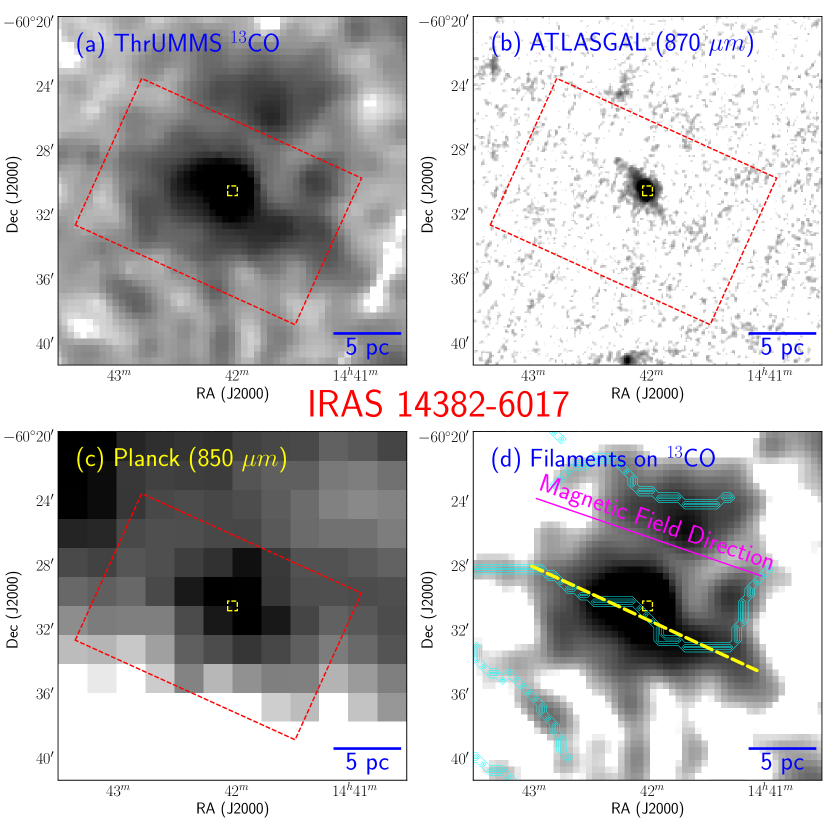
Figure 7.— Distribution of gas and dust in the IRAS 14382-6017 region. Filament is detected in the integrated ¹³CO and ATLASGAL 870 $\mu m$ images. Symbols are the same as in Figure 2.

Figure 7 (Cont.).— Distribution of gas and dust in the IRAS 14498-5856 region. Symbols are the same as in Figure 2.

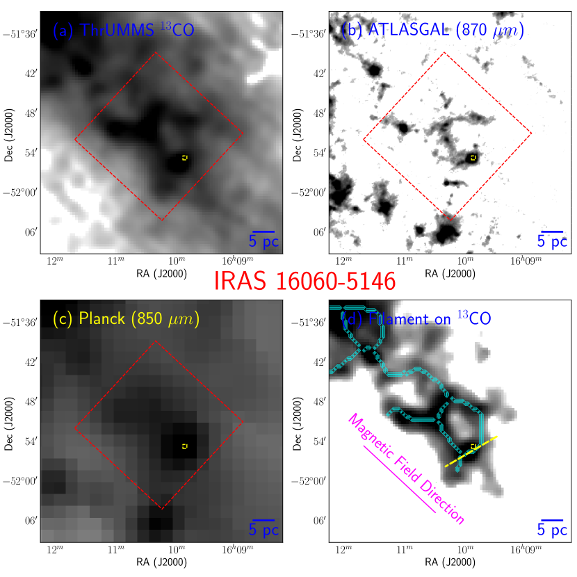
Figure 7 (Cont.).— Distribution of gas and dust in the IRAS 16060-5146 region. Symbols are the same as in Figure 2.

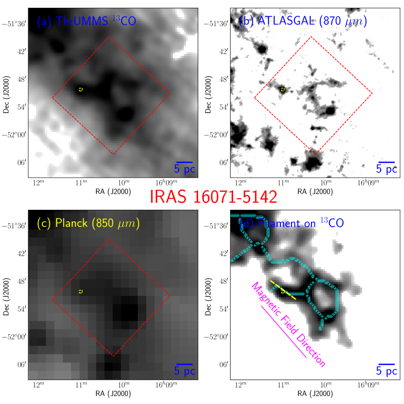
Figure 7 (Cont.).— Distribution of gas and dust in the IRAS 16071-5142 region. Symbols are the same as in Figure 2.

Figure 7 (Cont.).— Distribution of gas and dust in the IRAS 16076-5134 region. Symbols are the same as in Figure 2.

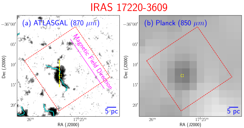
Figure 7 (Cont.).— Distribution of dust in the IRAS 17220-3609 region. Symbols are the same as in Figure 2.

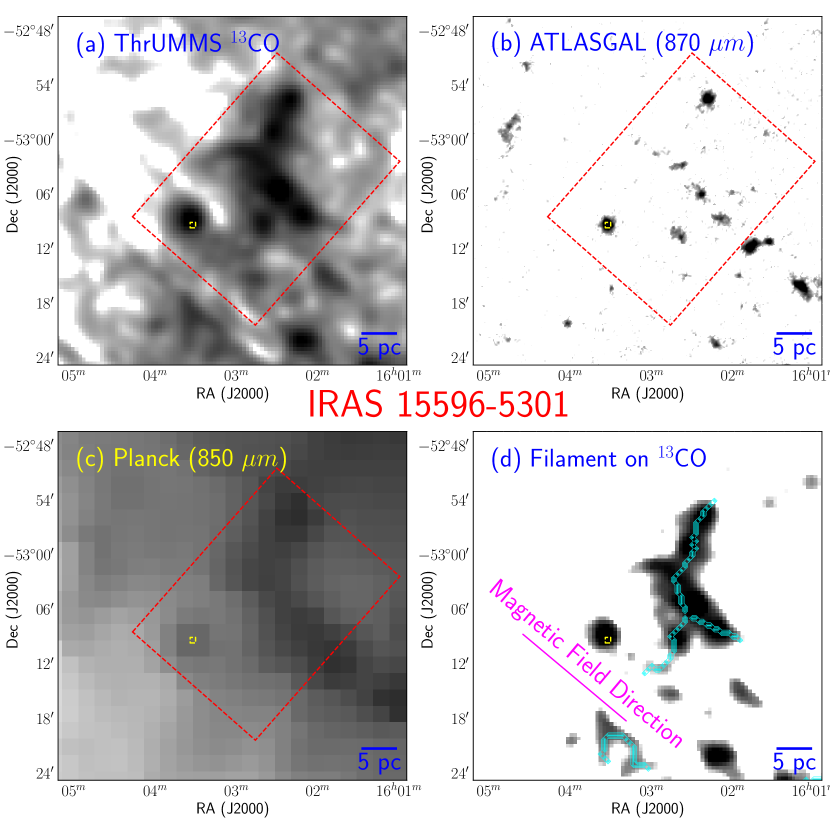
Figure 8 (Cont.).— Distribution of gas and dust in the IRAS 15596-5301 region where no filamentary structure is detected in the integrated ¹³CO and ATLASGAL 870 $\mu m$ images. Symbols are the same as in Figure 2.

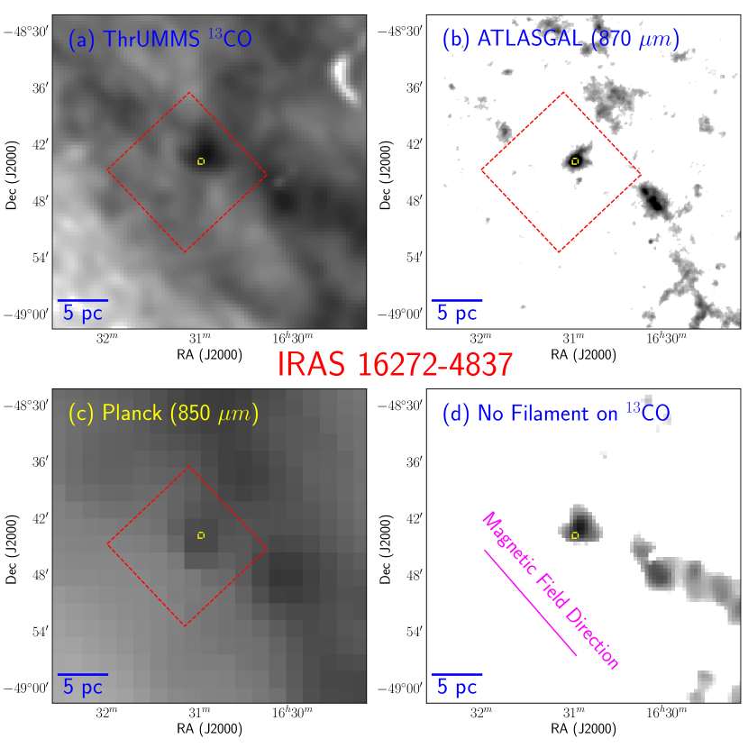
Figure 8 (Cont.).— Distribution of gas and dust in the IRAS 16272-4837 region. Symbols are the same as in Figure 2.

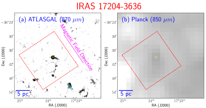
Figure 8 (Cont.).— Distribution of dust in the IRAS 17204-3636 region Symbols are the same as in Figure 2.

Appendix B B. Cumulative distribution of $\gamma_{\mathrm{Fil}}$

The cumulative distribution of $\gamma_{\mathrm{Fil}}$ (Figure 9 (Cont.)) after adding a random value within the uncertainty limit of $\pm$10$\arcdeg$.

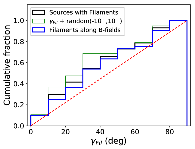
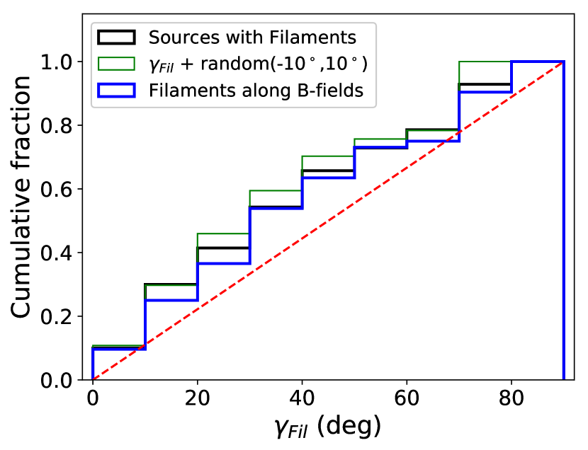
Figure 9 (Cont.).— Two examples of cumulative distribution functions of $\gamma_{Fil}$ with randomly added value within $\pm$10$\arcdeg$. No significant change is noted in the distribution.

References

- Anathpindika & Whitworth (2008) Anathpindika, S., & Whitworth, A. P. 2008, A&A, 487, 605
- André et al. (2010) André, P., Men’shchikov, A., Bontemps, S., et al. 2010, A&A, 518, L102
- André et al. (2014) André, P., Di Francesco, J., Ward-Thompson, D., et al. 2014, Protostars and Planets VI, 27
- Arce et al. (2011) Arce, H. G., Borkin, M. A., Goodman, A. A., et al. 2011, ApJ, 742, 105
- Arzoumanian et al. (2011) Arzoumanian, D., André, P., Didelon, P., et al. 2011, A&A, 529, L6
- Astropy Collaboration et al. (2018) Astropy Collaboration, Price-Whelan, A. M., Sipőcz, B. M., et al. 2018, AJ, 156, 123
- Bally (2016) Bally, J. 2016, ARA&A, 54, 491
- Barnes et al. (2015) Barnes, P. J., Muller, E., Indermuehle, B., et al. 2015, ApJ, 812, 6
- Baug et al. (2018) Baug, T., Dewangan, L. K., Ojha, D. K., et al. 2018, ApJ, 852, 119
- Bodenheimer (1995) Bodenheimer, P. 1995, ARA&A, 33, 199
- Busquet et al. (2013) Busquet, G., Zhang, Q., Palau, A., et al. 2013, ApJ, 764, L26
- Chapman et al. (2013) Chapman, N. L., Davidson, J. A., Goldsmith, P. F., et al. 2013, ApJ, 770, 151
- Clarke et al. (2017) Clarke, S. D., Whitworth, A. P., Duarte-Cabral, A., et al. 2017, MNRAS, 468, 2489
- Corradi et al. (1998) Corradi, R. L. M., Aznar, R., & Mampaso, A. 1998, MNRAS, 297, 617
- Dale & Bonnell (2011) Dale, J. E., & Bonnell, I. 2011, MNRAS, 414, 321
- Davis et al. (2009) Davis, C. J., Froebrich, D., Stanke, T., et al. 2009, A&A, 496, 153
- Faúndez et al. (2004) Faúndez, S., Bronfman, L., Garay, G., et al. 2004, A&A, 426, 97
- Fernández-López et al. (2014) Fernández-López, M., Arce, H. G., Looney, L., et al. 2014, ApJ, 790, L19
- Galametz et al. (2018) Galametz, M., Maury, A., Girart, J. M., et al. 2018, A&A, 616, A139
- Goodman et al. (1993) Goodman, A. A., Benson, P. J., Fuller, G. A., et al. 1993, ApJ, 406, 528
- Gray et al. (2018) Gray, W. J., McKee, C. F., & Klein, R. I. 2018, MNRAS, 473, 2124
- Hacar et al. (2013) Hacar, A., Tafalla, M., Kauffmann, J., et al. 2013, A&A, 554, A55
- Hull et al. (2014) Hull, C. L. H., Plambeck, R. L., Kwon, W., et al. 2014, ApJS, 213, 13
- Hull & Zhang (2019) Hull, C. L. H., & Zhang, Q. 2019, Frontiers in Astronomy and Space Sciences, 6, 3
- Kirk et al. (2013) Kirk, H., Myers, P. C., Bourke, T. L., et al. 2013, ApJ, 766, 115
- Koch & Rosolowsky (2015) Koch, E. W., & Rosolowsky, E. W. 2015, MNRAS, 452, 3435
- Kong et al. (2019) Kong, S., Arce, H. G., Maureira, M. J., et al. 2019, ApJ, 874, 104
- Kudoh, & Basu (2008) Kudoh, T., & Basu, S. 2008, ApJ, 679, L97
- Lee et al. (2014) Lee, K. I., Fernández-López, M., Storm, S., et al. 2014, ApJ, 797, 76
- Lee et al. (2016) Lee, K. I., Dunham, M. M., Myers, P. C., et al. 2016, ApJ, 820, L2
- Lee et al. (2017) Lee, J. W. Y., Hull, C. L. H., & Offner, S. S. R. 2017, ApJ, 834, 201
- Li et al. (2013) Li, H.-. bai ., Fang, M., Henning, T., et al. 2013, MNRAS, 436, 3707
- Li, H. et al. (2015) Li, H., Li, D., Qian, L., et al. 2015, ApJS, 219, 20
- Li, P.-S. et al. (2015) Li, P. S., McKee, C. F., & Klein, R. I. 2015, MNRAS, 452, 2500
- Li & Klein (2019) Li, P. S., & Klein, R. I. 2019, MNRAS, 485, 4509
- Liu et al. (2012) Liu, H. B., Jiménez-Serra, I., Ho, P. T. P., et al. 2012, ApJ, 756, 10
- Liu et al. (2016a) Liu, T., Zhang, Q., Kim, K.-T., et al. 2016, ApJ, 824, 31
- Liu et al. (2016b) Liu, T., Kim, K.-T., Yoo, H., et al. 2016, ApJ, 829, 59
- Lu et al. (2018) Lu, X., Zhang, Q., Liu, H. B., et al. 2018, ApJ, 855, 9
- Machida et al. (2005) Machida, M. N., Matsumoto, T., Hanawa, T., et al. 2005, MNRAS, 362, 382
- Machida et al. (2019) Machida, M. N., Hirano, S., & Kitta, H. 2019, ApJ, (arXiv:1911.03851)
- Matsumoto, & Tomisaka (2004) Matsumoto, T., & Tomisaka, K. 2004, ApJ, 616, 266
- Matthews, & Wilson (2000) Matthews, B. C., & Wilson, C. D. 2000, ApJ, 531, 868
- Myers (2009) Myers, P. C. 2009, ApJ, 700, 1609
- Offner et al. (2016) Offner, S. S. R., Dunham, M. M., Lee, K. I., et al. 2016, ApJ, 827, L11
- Pineda et al. (2011) Pineda, J. E., Arce, H. G., Schnee, S., et al. 2011, ApJ, 743, 201
- Pineda et al. (2015) Pineda, J. E., Offner, S. S. R., Parker, R. J., et al. 2015, Nature, 518, 213
- Planck Collaboration et al. (2016a) Planck Collaboration, Adam, R., Ade, P. A. R., et al. 2016, A&A, 594, A1
- Planck Collaboration et al. (2016b) Planck Collaboration, Adam, R., Ade, P. A. R., et al. 2016, A&A, 594, A8
- Planck Collaboration et al. (2016c) Planck Collaboration, Ade, P. A. R., Aghanim, N., et al. 2016, A&A, 586, A136
- Planck Collaboration et al. (2016d) Planck Collaboration, Ade, P. A. R., Aghanim, N., et al. 2016, A&A, 594, A19
- Reid et al. (2014) Reid, M. J., Menten, K. M., Brunthaler, A., et al. 2014, ApJ, 783, 130
- Santos et al. (2016) Santos, F. P., Busquet, G., Franco, G. A. P., et al. 2016, ApJ, 832, 186
- Schuller et al. (2009) Schuller, F., Menten, K. M., Contreras, Y., et al. 2009, A&A, 504, 415
- Siringo et al. (2009) Siringo, G., Kreysa, E., Kovács, A., et al. 2009, A&A, 497, 945
- Stephens et al. (2017) Stephens, I. W., Dunham, M. M., Myers, P. C., et al. 2017, ApJ, 846, 16
- Targon et al. (2011) Targon, C. G., Rodrigues, C. V., Cerqueira, A. H., et al. 2011, ApJ, 743, 54
- Tatematsu et al. (2016) Tatematsu, K., Ohashi, S., Sanhueza, P., et al. 2016, PASJ, 68, 24
- Wang et al. (2011) Wang, K., Zhang, Q., Wu, Y., et al. 2011, ApJ, 735, 64
- Wang et al. (2012) Wang, K., Zhang, Q., Wu, Y., et al. 2012, ApJ, 745, L30
- Wang et al. (2015) Wang, K., Testi, L., Ginsburg, A., et al. 2015, MNRAS, 450, 4043
- Wang et al. (2016) Wang, K., Testi, L., Burkert, A., et al. 2016, ApJS, 226, 9
- Wang (2018) Wang, Ke. 2018, Research Notes of the American Astronomical Society, 2, 52
- Wenger et al. (2018) Wenger, T. V., Balser, D. S., Anderson, L. D., & Bania, T. M. 2018, ApJ, 856, 52
- Yuan et al. (2018) Yuan, J., Li, J.-Z., Wu, Y., et al. 2018, ApJ, 852, 12
- Zhang et al. (2014) Zhang, Q., Qiu, K., Girart, J. M., et al. 2014, ApJ, 792, 116