Properties of Unique Information

Abstract.

We study the unique information function $UI(T:X\setminus Y)$ defined by Bertschinger et al. [4] within the framework of information decompositions. In particular, we study uniqueness and support of the solutions to the convex optimization problem underlying the definition of $UI$. We identify sufficient conditions for non-uniqueness of solutions with full support in terms of conditional independence constraints and in terms of the cardinalities of $T$, $X$ and $Y$. Our results are based on a reformulation of the first order conditions on the objective function as rank constraints on a matrix of conditional probabilities. These results help to speed up the computation of $UI(T:X\setminus Y)$, most notably when $T$ is binary. Optima in the relative interior of the optimization domain are solutions of linear equations if $T$ is binary. In the all binary case, we obtain a complete picture of where the optimizing probability distributions lie.

1. Introduction

Bertschinger et al. [4] introduced an information measure $UI(T:X\setminus Y)$ which they called unique information. The function $UI$ is proposed within the framework of information decompositions [17] to quantify the amount of information about $T$ that is contained in $X$ but not in $Y$. Similar quantities within this framework have been proposed by Harder et al. [8], Ince [9], James et al. [10] and Niu and Quinn [12]. Among them, the quantity $UI$ probably has the clearest axiomatic characterization. Although it has received a lot of attention by theorists [see e.g. 15, 2, 13], so far, applications have focused on other measures, because $UI$ is difficult to compute, although there has been recent progress [11, 3].

The function $UI$ is defined by means of an optimization problem. Let $T$, $X$, $Y$ be random variables with finite state spaces $\mathcal{T},\mathcal{X},\mathcal{Y}$ and with a joint distribution $P$. Let $\Delta_{\mathcal{T},\mathcal{X},\mathcal{Y}}$ be the set of all joint distributions of such random variables, and let

$$\Delta_{P}=\Big{\{}Q\in\Delta_{\mathcal{T},\mathcal{X},\mathcal{Y}}:Q(X=x,T=t)=P(X=x,T=t),\\ Q(Y=y,T=t)=P(Y=y,T=t)\text{ for all }x\in\mathcal{X},y\in\mathcal{Y},t\in\mathcal{T}\Big{\}}$$

be the set of all joint distributions that have the same pair marginals as $P$ for the pairs $(X,T)$ and $(Y,T)$. Then

(1) $$UI(T:X\setminus Y)=\min_{Q\in\Delta_{P}}I_{Q}(T:X|Y),$$

where $I_{Q}(T:X|Y)$ denotes the conditional mutual information of $T$ and $X$ given $Y$, computed with respect to $Q$. Due to the definition of $\Delta_{P}$, the optimization problem in (1) can be reformulated as follows:

(2) $$\min_{Q\in\Delta_{P}}I_{Q}(T:X|Y)=H(T|Y)-\max_{Q\in\Delta_{P}}H(T|X,Y).$$

This paper studies $UI$, focusing on the following two questions:

1. When is there a unique solution to the optimization problems in (2)?

2. When is there a solution in the relative interior of $\Delta_{P}$?

In the framework of information decomposition, the solutions to the optimization problems (2) are distributions with “zero synergy about $T$.” Thus, understanding these solutions sheds light on the concept of synergy. If the solution is unique, there is a unique way to combine the random variables $X$ and $Y$ without synergy about $T$ that preserves the $(X,T)$- and $(Y,T)$-marginals.

Moreover, a unique solution $Q^{*}$ might be used to “localize” the information decomposition, in the sense of Finn and Lizier [7]; although one should keep in mind that the support of $Q^{*}$ may satisfy $\operatorname{supp}(Q^{*})\not\supseteq\operatorname{supp}(P)$. A better understanding of the optimization problems also helps in the computation of $UI$. In the case where $\mathcal{T}$ is binary, an optimum in the interior of $\Delta_{P}$ can be found as solutions of linear equations. Solving an optimization problem can be avoided in the all binary case in which we derive a closed form solution of the optimization problem.

Summary of results and outline

Section 2 describes how the optimization domain $\Delta_{P}$ and its support depend on $P$.

Section 3 summarizes general facts about the optimization problem. The relationship between uniqueness of the optimizer and the supports of the optimizers is discussed, and sufficient conditions for non-uniqueness are identified.

Section 4 specializes to the case where $T$ is binary. In this case, if there is an optimizer in the interior, then this optimizer satisfies a conditional independence constraint. In general, the optimizer is not unique. We analyze how often the optimum lies in the interior or at the boundary of $\Delta_{P}$ and how often an optimum in the interior is unique as a function of the cardinalities of $\mathcal{X},\mathcal{Y}$ when sampling $P$ uniformly from $\Delta_{\mathcal{T},\mathcal{X},\mathcal{Y}}$.

Section 5 gives a complete picture for the case where all variables are binary. In this case, $\Delta_{P}$ is a rectangle, a line segment or a single point. A closed form expression is given for optimizers that lie in the interior of $\Delta_{P}$. If the optimizer does not lie in the interior, the optimum is attained at a vertex of $\Delta_{P}$.

Section 6 collects examples that demonstrate that the conditions of some of our results are indeed necessary. The final Section 7 presents our conclusions.

2. The optimization domain $\Delta_{P}$

Fix a joint distribution $P\in\Delta_{\mathcal{T},\mathcal{X},\mathcal{Y}}$. Since the marginal of $T$ is constant on $\Delta_{P}$, the support of $T$, which we denote by $\mathcal{T}^{\prime}:=\{t\in\mathcal{T}:P(T=t)>0\}$, is also constant on $\Delta_{P}$.

Any distribution $Q\in\Delta_{P}$ is characterized uniquely by the conditional probabilities $Q(X,Y|T=t)$ for $t\in\mathcal{T}^{\prime}$. The map

$$P\in\Delta_{\mathcal{T},\mathcal{X},\mathcal{Y}}\mapsto\big{(}P(X,Y|T=t)\big{)}_{t\in\mathcal{T}^{\prime}}$$

(where $\mathcal{T}^{\prime}$ depends on $P$) induces a linear bijection

$$\Delta_{P}=\operatorname*{\textnormal{\Large$\times$}}_{t\in\mathcal{T}^{\prime}}\Delta_{P,t},$$

where

$$\Delta_{P,t}=\Big{\{}Q\in\Delta_{\mathcal{X},\mathcal{Y}}:Q(X=x)=P(X=x |T=t),$$

$$Q(Y=y)=P(Y=y |T=t)\Big{\}},$$

and $\Delta_{\mathcal{X},\mathcal{Y}}$ is the set of all probability distributions of random variables $X,Y$ with finite state spaces $\mathcal{X},\mathcal{Y}$. For example, when $X$ and $Y$ are binary, $\Delta_{P,t}$ is a line segment (which may degenerate to a point) for all $t\in\mathcal{T}^{\prime}$. Thus, $\Delta_{P}$ is a product of line segments; that is, a hypercube (up to a scaling). If $T$ is also binary, then $\Delta_{P}$ is a rectangle (a product of two line segments), which may degenerate to a line segment or even a point depending on the support of $P$. A figure of $\Delta_{P}$ in the case that all variables are binary (when $\Delta_{P}$ is a rectangle) can be found in[4]. Figure 1 makes use of the product structure to visualize $\Delta_{P}$ in the case $|\mathcal{T}|=2=|\mathcal{X}|$, $|\mathcal{Y}=3|$, where $\dim(\Delta_{P})=4$.

In the following, for $Q\in\Delta_{P}$ and $t\in\mathcal{T}^{\prime}$, we write $Q_{t}:=Q(X,Y|T=t)$ for the conditional distribution of $X,Y$ given that $T=t$. The product structure of $\Delta_{P}$ implies: if $Q\in\Delta_{P}$ lies on the boundary of $\Delta_{P}$, then at least one of the $Q_{t}$ lies on the boundary of $\Delta_{P,t}$. Moreover, $Q$ lies on the boundary of $\Delta_{\mathcal{T},\mathcal{X},\mathcal{Y}}$. Hence, the boundaries of the polytopes $\Delta_{P}$ or $\Delta_{P,t}$ are characterized by the vanishing of probabilities.

Remark 2.1.

In the following, the expression boundary of $\Delta_{P}$ refers to the relative boundary. If $P$ lies on the boundary of $\Delta_{\mathcal{T},\mathcal{X},\mathcal{Y}}$, then $\Delta_{P}$ may be a subset of the boundary of $\Delta_{\mathcal{T},\mathcal{X},\mathcal{Y}}$ (cf. Lemma 2.4). This happens if and only if one probability vanishes throughout $\Delta_{P,t}$ (and thus one probability vanishes throughout $\Delta_{P}$). In this case, $\Delta_{P}$ is part of the boundary of $\Delta_{\mathcal{T},\mathcal{X},\mathcal{Y}}$. However, the (relative) boundary of $\Delta_{P}$ is a strict subset of $\Delta_{P}$, and the same holds for $\Delta_{P,t}$.

Let $A$ be the linear map that maps a joint distribution $P\in\Delta_{\mathcal{T},\mathcal{X},\mathcal{Y}}$ to the pair $(P(X,T),P(Y,T))$ of marginal distributions. Then

$$\Delta_{P}=(P+\ker(A))\cap\Delta_{\mathcal{T},\mathcal{X},\mathcal{Y}}.$$

The difference of any two elements of $\Delta_{P}$ belongs to $\ker(A)$. Conversely, the elements of $\ker(A)$ can be used to move within each $\Delta_{P}$. A generating set of $\ker(A)$ is given by the vectors

(3) $$\gamma_{t;x,x^{\prime};y,y^{\prime}}=\delta_{t,x,y}+\delta_{t,x^{\prime},y^{\prime}}-\delta_{t,x,y^{\prime}}-\delta_{t,x^{\prime},y},\qquad x,x^{\prime}\in\mathcal{X},y,y^{\prime}\in\mathcal{Y},t\in\mathcal{T}$$

where $\delta_{t,x,y}$ denotes the Dirac measure supported at $T=t,X=x,Y=y$. These vectors are not linearly independent. One way to choose a linearly independent subset is to fix $x_{0}\in\mathcal{X}$, $y_{0}\in\mathcal{Y}$. Then the set

$$\Gamma:=\big{\{}\gamma_{t;x,x_{0};y,y_{0}}:x\in\mathcal{X}\setminus\{x_{0}\},y\in\mathcal{Y}\setminus\{y_{0}\},t\in\mathcal{T}\big{\}}$$

is a basis of $\ker(A)$.

Remark 2.2.

Apart from being symmetric, the larger dependent set has the following advantage, which is reminiscent of the Markov basis property [5]: Any two points $Q,Q^{\prime}\in\Delta_{P}$ can be connected by a path in $\Delta_{P}$ by applying a sequence of multiples of the elements $\gamma_{t;x,x^{\prime};y,y^{\prime}}$. The same is not true if we restrict $x^{\prime},y^{\prime}$ to $x_{0},y_{0}$: if $Q(X=x_{0})=0$, then adding a multiple of $\gamma_{t;x,x_{0};y,y_{0}}$ for any $x\in\mathcal{X}$, $y\in\mathcal{Y}$ leads to a negative entry.

Let $V$ be the set of distributions $Q_{0}\in\Delta_{\mathcal{T},\mathcal{X},\mathcal{Y}}$ that have a factorization of the form

$$Q_{0}(t,x,y)=Q_{0}(t)Q_{0}(x|t)Q_{0}(y|t).$$

Thus, $V$ consists of all joint distributions that satisfy the Markov chain $X\;\text{--}\;T\;\text{--}\;Y$. For each $P\in\Delta_{\mathcal{T},\mathcal{X},\mathcal{Y}}$, the intersection $\Delta_{P}\cap V$ contains precisely one element $Q_{0}=Q_{0}(P)$; namely

(4) $$Q_{0}(t,x,y)=P(t)P(x|t)P(y|t).$$

In the language of information geometry, $\Delta_{P}$ is a linear family that is dual to the exponential family $V$ [1]. A general distribution $Q\in\Delta_{\mathcal{T},\mathcal{X},\mathcal{Y}}$ can thus be expressed uniquely in the form

(5) $$Q=Q_{0}+\sum_{t,x^{\prime},y^{\prime}}P(t)g_{t,x^{\prime},y^{\prime}}\gamma_{t;x,x^{0};y,y^{0}}$$

with $Q_{0}=Q_{0}(Q)\in V$ and $g=(g_{t,x^{\prime},y^{\prime}})_{t,x^{\prime}\neq x^{0},y^{\prime}\neq y^{0}}$ denoting the coefficients with respect to $\Gamma$.

Let $\operatorname{supp}(\Delta_{P}):=\bigcup_{Q\in\Delta_{P}}\operatorname{supp}(Q)$ be the largest support of an element of $\Delta_{P}$. Generic elements of $\Delta_{P}$ have support $\operatorname{supp}(\Delta_{P})$. We also let

$$\operatorname{supp}(\Delta_{P,t}):=\bigcup_{Q\in\Delta_{P}}\operatorname{supp}(Q_{t})\\ =\big{\{}(x,y)\in\mathcal{X}\times\mathcal{Y}:(t,x,y)\in\operatorname{supp}(\Delta_{P})\big{\}}\text{ for~{}$t\in\mathcal{T}^{\prime}$.}$$

If $\Delta_{P}$ is a singleton, then $P=Q_{0}$. In this case, $\operatorname{supp}(\Delta_{P})=\operatorname{supp}(P)$, and $\operatorname{supp}(\Delta_{P,t})=\operatorname{supp}(P_{t})$.

For $t\in\mathcal{T}^{\prime}$ let $\mathcal{X}_{t}=\big{\{}x\in\mathcal{X}:P(X=x|T=t)>0\big{\}}$ and $\mathcal{Y}_{t}=\big{\{}y\in\mathcal{Y}:P(Y=y|T=t)>0\}$. It follows from the definitions:

Lemma 2.3.

Let $t\in\mathcal{T}^{\prime}$. Then $\operatorname{supp}(\Delta_{P,t})=\operatorname{supp}(Q_{0,t})=\mathcal{X}_{t}\times\mathcal{Y}_{t}$. Moreover, $\operatorname{supp}(\Delta_{P})=\operatorname{supp}(Q_{0})$. Thus, $Q_{0}$ has maximal support in $\Delta_{P}$.

The next lemma follows from Lemma 2.3 and the definitions:

Lemma 2.4.

Let $t\in\mathcal{T}$, $x\in\mathcal{X}$ and $y\in\mathcal{Y}$. The following statements are equivalent:

1. $\Delta_{P}$ lies in the face of $\Delta_{\mathcal{T},\mathcal{X},\mathcal{Y}}$ defined by $Q(t,x,y)=0$.

2. $(t,x,y)\notin\operatorname{supp}(\Delta_{P})$.

3. Every $Q\in\Delta_{P}$ satisfies $Q(t,x,y)=0$.

4. $Q_{0}:=Q_{0}(P)$ satisfies $Q_{0}(t,x,y)=0$.

5. $P(T=t,Y=y)P(T=t,X=x)=0$.

Lemma 2.5.

Let $t\in\mathcal{T}^{\prime}$. The following are equivalent:

1. $\Delta_{P,t}$ is a singleton.

2. At least one of $\mathcal{X}_{t}$, $\mathcal{Y}_{t}$ is a singleton.

Proof.

Condition 2. in the lemma captures precisely when it is not possible to add a multiple of some $\gamma_{t;x,x^{\prime};y,y^{\prime}}$ to $P$ or, in fact, to any $Q\in\Delta_{P}$ (cf. Remark 2.2). ∎

3. Support and uniqueness of the optimum

This section studies the uniqueness of the optimizer and the question, when it lies on the boundary of $\Delta_{P}$. There are many relations between uniqueness and support of the optimizers: Lemma 3.1 states that, if the optimizer is not unique, then there are optimizers with restricted support. Theorems 3.6, 3.7, 3.8 and 3.10 prove that either the optimizer lies at the boundary or it is not unique under a variety of different assumptions that involve the cardinalities of $|\mathcal{X}|$, $|\mathcal{Y}|$ and $|\mathcal{T}|$ or conditional independence conditions.

Lemma 3.1.

If the optimizer is not unique, then there exists an optimizer on the boundary of $\Delta_{P}$.

Proof.

Suppose that there are two distinct optimizers $Q_{1},Q_{2}\in\Delta_{P}$, and assume that neither $Q_{1}$ nor $Q_{2}$ lies on the boundary of $\Delta_{P}$. By convexity of the target function $I_{Q}(T:X|Y)$ on $\Delta_{P}$ (see Lemma 4 in [4] or Lemma 3.4 below), the convex hull of $Q_{1}$ and $Q_{2}$ consists of optimizers. Let $L_{Q_{1},Q_{2}}$ be the line through $Q_{1},Q_{2}$. The target function $I_{Q}(T:X|Y)$ is a continuous function on the line segment $L_{Q_{1},Q_{2}}\cap\Delta_{P}$, and it is analytic on the relative interior of this line segment. By assumption, $I_{Q}(T:X|Y)$ is constant on the part of $L_{Q_{1},Q_{2}}$ between $Q_{1}$ and $Q_{2}$. By the principle of permanence, $I_{Q}(T:X|Y)$ is constant on $L_{Q_{1},Q_{2}}\cap\Delta_{P}$. Therefore, the two points where $L_{Q_{1},Q_{2}}$ intersect the boundary of $\Delta_{P}$ are optimizers of $I_{Q}(T:X|Y)$ that lie on the boundary of $\Delta_{P}$. ∎

The derivative of $I_{Q}(T:X|Y)$ in the direction of $\gamma_{t;x,x^{\prime};y,y^{\prime}}$ at $Q$ equals

(6) $$\log\left(\frac{Q(t,x,y)Q(t,x^{\prime},y^{\prime})}{Q(t,x,y^{\prime})Q(t,x^{\prime},y)}\cdot\frac{Q(x,y^{\prime})Q(x^{\prime},y)}{Q(x,y)Q(x^{\prime},y^{\prime})}\right)=\log\left(\frac{Q(t|x,y)Q(t|x^{\prime},y^{\prime})}{Q(t|x,y^{\prime})Q(t|x^{\prime},y)}\right),$$

assuming that the probabilities in the logarithm are positive. Otherwise, the partial derivative has to be computed as a limit.

Remark 3.2.

The vanishing of the directional derivative of $I_{Q}(T:X|Y)$ can be seen as a determinantal condition: all derivatives (6) vanish if and only if for all $t\in\mathcal{T}^{\prime}$ the determinants of all $2\times 2$-submatrices of the matrix $(Q(t|x,y))_{x,y}\in\mathbb{R}^{\mathcal{X}\times\mathcal{Y}}$ vanish; that is, if and only if these matrices have rank one. As $\sum_{t\in\mathcal{T}^{\prime}}Q(t|x,y)=1$ for all $x,y$, the sum of these rank-one matrices is again of rank one.

Conversely, let $\tilde{Q}_{1},\dots,\tilde{Q}_{k}$ be non-negative rank-one matrices such that the sum $\tilde{Q}=\tilde{Q}_{1}+\dots+\tilde{Q}_{k}$ is non-zero and again of rank one; say $\tilde{Q}=vw^{\top}$ with $v,w$ non-negative and $\top$ denoting the transpose. Let $V=\operatorname{diag}(v)$, $W=\operatorname{diag}(w)$, and let $Q_{t}=V^{-1}\tilde{Q}_{t}W^{-1}$ for $t=1,\dots,k$. Then $Q_{1}+\dots+Q_{k}=V^{-1}\tilde{Q}W^{-1}$ is the matrix with all entries equal to one. Thus, the matrices $Q_{t}$ for $t=1,\dots,k$ can be interpreted as matrices of conditional probabilities $Q(t|X,Y)$. Together with any distribution of the pair $(X,Y)$, one obtains a distribution $Q(T,X,Y)$ at which all directional derivatives of $I_{Q}(T:X|Y)$ vanish.

Lemma 3.3.

Let $Q^{*}$ be a minimizer of $I_{Q}(T:X|Y)$ for $Q\in\Delta_{P}$, and let $(t,x,y)\in\operatorname{supp}(\Delta_{P})$. If $Q^{*}(t,x,y)=0$, then $Q^{*}(x,y)=0$. Thus, $Q^{*}(t^{\prime},x,y)=0$ for all $t^{\prime}\in\mathcal{T}$.

Proof.

Suppose that $Q^{*}(t,x,y)=0$, but that $Q^{*}(x,y)>0$. Then there exist $x^{\prime},y^{\prime}$ such that $Q_{\epsilon}:=Q^{*}+\epsilon\gamma_{t;x,x^{\prime};y,y^{\prime}}$ is non-negative for $\epsilon>0$ small enough (and thus $Q_{\epsilon}\in\Delta_{P}$). In particular, $Q^{*}(t,x^{\prime},y),Q^{*}(t,x,y^{\prime})>0$.

Since $Q^{*}$ is a minimizer, the partial derivative (6) at $Q^{*}$ must be non-negative. Note that, by assumption, $Q^{*}(t,x,y)=0$. If all four probabilities in the denominator of the fraction in the logarithm were non-zero, then the partial derivative would be equal to minus infinity. Thus, either $Q^{*}(x,y)$ or $Q^{*}(x^{\prime},y^{\prime})$ must vanish.

Suppose that $Q^{*}(x,y)>0$. Then $Q^{*}(x^{\prime},y^{\prime})=0$. Hence, $Q^{*}(t,x^{\prime},y^{\prime})=0$, and so

$$\frac{Q_{\epsilon}(t,x,y)Q_{\epsilon}(t,x^{\prime},y^{\prime})}{Q_{\epsilon}(t,x,y^{\prime})Q_{\epsilon}(t,x^{\prime},y)}\cdot\frac{Q_{\epsilon}(x,y^{\prime})Q\epsilon(x^{\prime},y)}{Q_{\epsilon}(x,y)Q_{\epsilon}(x^{\prime},y^{\prime})}\\ =\frac{\epsilon^{2}Q_{\epsilon}(x,y^{\prime})Q_{\epsilon}(x^{\prime},y)}{Q_{\epsilon}(t,x,y^{\prime})Q_{\epsilon}(t,x^{\prime},y)Q_{\epsilon}(x,y)\epsilon}=O(\epsilon).$$

Thus, the partial derivative diverges as $\log(\epsilon)$ to $-\infty$ as $\epsilon\to 0$, contradicting the fact that $Q^{*}$ is a local minimizer. Therefore, $Q^{*}(x,y)=0$. ∎

If $Q^{*}(t,x,y)=0$ and $Q^{*}(t,x^{\prime},y)>0$, $Q^{*}(t,x,y^{\prime})>0$ for some $t\in\mathcal{T}^{\prime}$, $x,x^{\prime}\in\mathcal{X}$, $y,y^{\prime}\in\mathcal{Y}$, then the partial derivative at $Q^{*}$ in the direction of $\gamma_{t;x,x^{\prime};y,y^{\prime}}$ is

$$\log\left(\frac{Q^{*}(t,x^{\prime},y^{\prime})Q^{*}(x,y^{\prime})Q^{*}(x^{\prime},y)}{Q^{*}(t,x,y^{\prime})Q^{*}(t,x^{\prime},y)Q^{*}(x^{\prime},y^{\prime})}\right).$$

Therefore,

$$Q^{*}(t,x^{\prime},y^{\prime})Q^{*}(x,y^{\prime})Q^{*}(x^{\prime},y)\geq Q^{*}(t,x,y^{\prime})Q^{*}(t,x^{\prime},y)Q^{*}(x^{\prime},y^{\prime}),$$

or

$$\frac{Q^{*}(t,x^{\prime},y^{\prime})}{Q^{*}(x^{\prime},y^{\prime})}\geq\frac{Q^{*}(t,x,y^{\prime})}{Q^{*}(x,y^{\prime})}\frac{Q^{*}(t,x^{\prime},y)}{Q^{*}(x^{\prime},y)}.$$

It is well known that entropy is strictly concave and that conditional entropy is concave. From the proof of this fact, it is easy to analyze where conditional entropy is strictly concave.

Lemma 3.4.

The conditional entropy $H(A|B)$ is concave in the joint distribution of $A,B$. It is strictly concave, with the exception of those directions where $P(A|B)$ is constant. That is:

$$\lambda H_{P_{1}}(A|B)+(1-\lambda)H_{P_{2}}(A|B)\leq H_{\lambda P_{1}+(1-\lambda)P_{2}}(A|B)$$

with equality if and only if $P_{1}(A|B)=P_{2}(A|B)$ a.e.

Proof.

Let $\theta$ be a Bernoulli random variable with parameter $\lambda$, and consider the joint distribution $P$ of $\theta$, $A$ and $B$ given by

$$P(A,B,\theta)=\begin{cases}\lambda P_{1}(A,B),&\text{ if }\theta=0,\\ (1-\lambda)P_{2}(A,B),&\text{ if }\theta=1.\end{cases}$$

Then

$$H_{\lambda P_{1}+(1-\lambda)P_{2}}(A|B)=H_{P}(A|B)\geq H_{P}(A|B,\theta)\\ =\lambda H_{P_{1}}(A|B)+(1-\lambda)H_{P_{2}}(A|B).$$

Equality holds if and only if $A$ is independent of $\theta$ given $B$; that is:

$$P_{1}(A|B)=P(A|B,\theta=0)=P(A|B,\theta=1)=P_{2}(A|B).\qed$$

Lemma 3.5.

Let $Q_{1},Q_{2}\in\Delta_{P}$ be two maximizers of $\max_{Q\in\Delta_{P}}H_{Q}(T|XY)$. Then $Q_{1}(T|XY)=Q_{2}(T|XY)$.

Proof.

We may assume that $Q_{1}\neq Q_{2}$. By assumption, $H_{Q}(T|XY)$ is constant on the line segment between $Q_{1}$ and $Q_{2}$. Thus, on this line segment $H_{Q}(T|XY)$ is not strictly concave. By Lemma 3.4, $Q_{1}(T|XY)=Q_{2}(T|XY)$. ∎

The following four theorems give different sufficient conditions for non-uniqueness of the optimizer.

Theorem 3.6.

Suppose that $|\mathcal{T}|<\min\big{\{}|\mathcal{X}|,|\mathcal{Y}|\big{\}}$. If there exists an optimizer of $\max_{Q\in\Delta_{P}}H_{Q}(T|XY)$ with full support, then the optimizer is not unique.

Proof.

Suppose that $Q^{*}\in\arg\max_{Q\in\Delta_{P}}H_{Q}(T|XY)$ has full support. The proof proceeds by finding a direction within $\Delta_{P}$ in which $H_{Q}(T|XY)$ is not strictly concave. Consider the linear equation

(7) $$Q(t,x,y)=Q^{*}(t|x,y)Q(x,y)\quad\text{ for }Q\in\Delta_{P}.$$

If $Q^{\prime}\in\Delta_{P}$ solves this equation, then, by Lemma 3.4, the function $H_{Q}(T|X,Y)$ is affine on the line connecting $Q^{*}$ and $Q^{\prime}$. Since $Q^{*}$ is a maximizer, $H_{Q}(T|X,Y)$ is constant on this line, whence any point on this line is a maximizer. Thus, to prove the theorem, it suffices to show that there exists a solution $Q^{\prime}\neq Q*$ in $\Delta_{P}$ to (7).

By Remark 3.2, for every $t\in\mathcal{T}^{\prime}$, there exists a pair of non-negative vectors $v_{t},w_{t}$ such that $Q^{*}(t|x,y)=v_{t}w_{t}^{\top}$. The assumption $|\mathcal{T}|<\min\big{\{}|\mathcal{X}|,|\mathcal{Y}|\big{\}}$ implies that there exist non-zero $v_{0}\in\mathbb{R}^{\mathcal{X}}$, $w_{0}\in\mathbb{R}^{\mathcal{Y}}$ with $v_{0}^{\top}v_{t}=0=w_{0}^{\top}w_{t}$ for all $t\in\mathcal{T}^{\prime}$. For $\epsilon\in\mathbb{R}$ let

$$Q_{\epsilon}(x,y):=Q^{*}(x,y)+\epsilon v_{0,x}^{\top}w_{0,y}.$$

Then

$$\sum_{x\in\mathcal{X},y\in\mathcal{Y}}Q_{\epsilon}(x,y)=\sum_{x\in\mathcal{X},y\in\mathcal{Y}}Q^{*}(x,y)+\epsilon\sum_{x\in\mathcal{X},y\in\mathcal{Y}}v_{0,x}w_{0,y}=1,$$

because

$$\sum_{x\in\mathcal{X},y\in\mathcal{Y}}v_{0,x}w_{0,y}=\sum_{x\in\mathcal{X},y\in\mathcal{Y}}v_{0,x}w_{0,y}\sum_{t\in\mathcal{T}^{\prime}}Q^{*}(t|x,y)\\ =\sum_{t\in\mathcal{T}^{\prime}}\sum_{x\in\mathcal{X}}v_{0,x}v_{t,x}\sum_{y\in\mathcal{Y}}w_{0,y}w_{t,y}=0.$$

Therefore, if $\epsilon$ is sufficiently close to zero, then $Q_{\epsilon}$ defines a probability distribution for $X$ and $Y$.

Extend $Q_{\epsilon}$ to a joint distribution of $T,X,Y$ by $Q_{\epsilon}(t,x,y)=Q^{*}(t|x,y)Q_{\epsilon}(x,y)$. Then $Q_{\epsilon}$ satisfies (7). It remains to show that $Q_{\epsilon}\in\Delta_{Q^{*}}$. From

$$Q_{\epsilon}(t,x)-Q^{*}(t,x)=\sum_{y\in\mathcal{Y}}\big{(}Q_{\epsilon}(t,x,y)-Q^{*}(t,x,y)\big{)}\\ =\sum_{y\in\mathcal{Y}}Q^{*}(t|x,y)\big{(}Q_{\epsilon}(x,y)-Q^{*}(x,y)\big{)}=\epsilon v_{t,x}v_{0,x}\sum_{y\in\mathcal{Y}}w_{t,y}w_{0,y}=0$$

follows $Q_{\epsilon}(T,X)=Q^{*}(T,X)$. The equality $Q_{\epsilon}(T,Y)=Q^{*}(T,Y)$ follows similarly. ∎

Theorem 3.7.

Let $|\mathcal{T}|<|\mathcal{Y}|$, and suppose that $UI(T:X\setminus Y)=0$. If there is an optimizer of $\max_{Q\in\Delta_{P}}H_{Q}(T|X,Y)$ with full support, then the optimizer is not unique.

Proof.

The proof of Theorem 3.6 can be adapted. Under the assumptions of the theorem, if $Q^{*}$ is an optimizer, then $Q^{*}(t|x,y)=Q^{*}(t|y)$ does not depend on $x$. Therefore, one may choose $v_{t,x}=1$ for all $y\in\mathcal{Y},t\in\mathcal{T}$ and $w_{t,y}=Q^{*}(t|y)$. To construct $v_{0}$, it now suffices that $|\mathcal{X}|\geq 2$, since all vectors $v_{t}$, $t\in\mathcal{T}$, are identical. ∎

Theorem 3.8.

Suppose that $H(X),H(Y)>0$. If both $\left.T\mathchoice{\mathrel{\hbox to0.0pt{$\displaystyle\perp$\hss}\mkern 2.0mu{\displaystyle\perp}}}{\mathrel{\hbox to0.0pt{$\textstyle\perp$\hss}\mkern 2.0mu{\textstyle\perp}}}{\mathrel{\hbox to0.0pt{$\scriptstyle\perp$\hss}\mkern 2.0mu{\scriptstyle\perp}}}{\mathrel{\hbox to0.0pt{$\scriptscriptstyle\perp$\hss}\mkern 2.0mu{\scriptscriptstyle\perp}}}\!\!_{\smash{P}}\;X\right.$ and $\left.T\mathchoice{\mathrel{\hbox to0.0pt{$\displaystyle\perp$\hss}\mkern 2.0mu{\displaystyle\perp}}}{\mathrel{\hbox to0.0pt{$\textstyle\perp$\hss}\mkern 2.0mu{\textstyle\perp}}}{\mathrel{\hbox to0.0pt{$\scriptstyle\perp$\hss}\mkern 2.0mu{\scriptstyle\perp}}}{\mathrel{\hbox to0.0pt{$\scriptscriptstyle\perp$\hss}\mkern 2.0mu{\scriptscriptstyle\perp}}}\!\!_{\smash{P}}\;Y\right.$, then $\arg\max_{Q\in\Delta_{P}}{H_{Q}(T|X,Y)}$ is not unique.

Proof.

Let $Q_{0}=Q_{0}(P)=P_{T}P_{X|T}P_{Y|T}=P_{T}P_{X}P_{Y}\in\Delta_{P}$. Then $\left.T\mathchoice{\mathrel{\hbox to0.0pt{$\displaystyle\perp$\hss}\mkern 2.0mu{\displaystyle\perp}}}{\mathrel{\hbox to0.0pt{$\textstyle\perp$\hss}\mkern 2.0mu{\textstyle\perp}}}{\mathrel{\hbox to0.0pt{$\scriptstyle\perp$\hss}\mkern 2.0mu{\scriptstyle\perp}}}{\mathrel{\hbox to0.0pt{$\scriptscriptstyle\perp$\hss}\mkern 2.0mu{\scriptscriptstyle\perp}}}\!\!_{\smash{Q_{0}}}\;(X,Y)\right.$ by construction. Since $H_{Q}(T|X,Y)\leq H(T)$ for $Q\in\Delta_{P}$ and since $Q_{0}$ achieves equality, $Q_{0}$ maximizes $H(T|X,Y)$ on $\Delta_{P}$.

Due to the assumption of positive entropy, there exist $x_{0},x_{1}\in\mathcal{X}$, $y_{0},y_{1}\in\mathcal{Y}$ with $P_{X}(x_{0})>0$, $P_{X}(x_{1})>0$, $P_{Y}(y_{0})>0$ and $P_{Y}(y_{1})>0$. For $\delta\in\mathbb{R}$ let

$$Q_{\delta}(t,x,y):=Q_{0}(t,x,y)+\delta p_{T}(t)\gamma_{t;x_{0},x_{1};y_{0},y_{1}}.$$

If $|\delta|$ is small enough, then $Q_{\delta}$ is non-negative and hence belongs to $\Delta_{P}$. For such $\delta$, the conditional $Q_{\delta}(x,y|t)$ does not depend on $t$, whence $\left.T\mathchoice{\mathrel{\hbox to0.0pt{$\displaystyle\perp$\hss}\mkern 2.0mu{\displaystyle\perp}}}{\mathrel{\hbox to0.0pt{$\textstyle\perp$\hss}\mkern 2.0mu{\textstyle\perp}}}{\mathrel{\hbox to0.0pt{$\scriptstyle\perp$\hss}\mkern 2.0mu{\scriptstyle\perp}}}{\mathrel{\hbox to0.0pt{$\scriptscriptstyle\perp$\hss}\mkern 2.0mu{\scriptscriptstyle\perp}}}\!\!_{\smash{Q_{\delta}}}\;(X,Y)\right.$. Thus, all such $Q_{\delta}$ are maximizers of $H_{Q}(T|X,Y)$ for $Q\in\Delta_{P}$. ∎

Example 3.9.

Let $P$ be the distribution of three independent uniform binary random variables $T,X,Y$, and let $P^{\prime}$ be the joint distribution where $X,T$ are uniform independent binary random variables and where $X=Y$. Then $\Delta_{P}=\Delta_{P^{\prime}}$, and both $P$ and $P^{\prime}$ maximize $H_{Q}(T|X,Y)$ for $Q\in\Delta_{P}$.

This example is the same as Example 31 by Bertschinger et al. [4]. Ironically, Bertschinger et al. [4] remarked that the optimization problem is ill-conditioned, but they failed to observe the non-uniqueness of the optimum in this case.

The following technical result generalizes Theorem 3.8. It is illustrated by Example 6.2.

Theorem 3.10.

Suppose that $\left.T\mathchoice{\mathrel{\hbox to0.0pt{$\displaystyle\perp$\hss}\mkern 2.0mu{\displaystyle\perp}}}{\mathrel{\hbox to0.0pt{$\textstyle\perp$\hss}\mkern 2.0mu{\textstyle\perp}}}{\mathrel{\hbox to0.0pt{$\scriptstyle\perp$\hss}\mkern 2.0mu{\scriptstyle\perp}}}{\mathrel{\hbox to0.0pt{$\scriptscriptstyle\perp$\hss}\mkern 2.0mu{\scriptscriptstyle\perp}}}\!\!_{\smash{P}}\;X\,\middle|\,Y\right.{}$ and $\left.T\mathchoice{\mathrel{\hbox to0.0pt{$\displaystyle\perp$\hss}\mkern 2.0mu{\displaystyle\perp}}}{\mathrel{\hbox to0.0pt{$\textstyle\perp$\hss}\mkern 2.0mu{\textstyle\perp}}}{\mathrel{\hbox to0.0pt{$\scriptstyle\perp$\hss}\mkern 2.0mu{\scriptstyle\perp}}}{\mathrel{\hbox to0.0pt{$\scriptscriptstyle\perp$\hss}\mkern 2.0mu{\scriptscriptstyle\perp}}}\!\!_{\smash{P}}\;Y\,\middle|\,X\right.{}$. If there exist $x_{0}\in\mathcal{X}$, $y_{0}\in\mathcal{Y}$ with $P(X=x_{0},Y=y_{0})>0$ and $H(X|Y=y_{0})\neq 0\neq H(Y|X=x_{0})$, then $\max_{Q\in\Delta_{P}}{H_{Q}(T|X,Y)}$ is not unique.

Proof.

If $\left.T\mathchoice{\mathrel{\hbox to0.0pt{$\displaystyle\perp$\hss}\mkern 2.0mu{\displaystyle\perp}}}{\mathrel{\hbox to0.0pt{$\textstyle\perp$\hss}\mkern 2.0mu{\textstyle\perp}}}{\mathrel{\hbox to0.0pt{$\scriptstyle\perp$\hss}\mkern 2.0mu{\scriptstyle\perp}}}{\mathrel{\hbox to0.0pt{$\scriptscriptstyle\perp$\hss}\mkern 2.0mu{\scriptscriptstyle\perp}}}\!\!_{\smash{P}}\;X\,\middle|\,Y\right.{}$, then $I_{P}(T:X|Y)=0$. From this it follows that $P$ belongs to $\arg\min_{Q\in\Delta_{P}}I_{Q}(T:X|Y)=\arg\max_{Q\in\Delta_{P}}H_{Q}(T|XY)$. The probability distributions that satisfy $\left.T\mathchoice{\mathrel{\hbox to0.0pt{$\displaystyle\perp$\hss}\mkern 2.0mu{\displaystyle\perp}}}{\mathrel{\hbox to0.0pt{$\textstyle\perp$\hss}\mkern 2.0mu{\textstyle\perp}}}{\mathrel{\hbox to0.0pt{$\scriptstyle\perp$\hss}\mkern 2.0mu{\scriptstyle\perp}}}{\mathrel{\hbox to0.0pt{$\scriptscriptstyle\perp$\hss}\mkern 2.0mu{\scriptscriptstyle\perp}}}\!\!_{\smash{P}}\;X\,\middle|\,Y\right.{}$ and $\left.T\mathchoice{\mathrel{\hbox to0.0pt{$\displaystyle\perp$\hss}\mkern 2.0mu{\displaystyle\perp}}}{\mathrel{\hbox to0.0pt{$\textstyle\perp$\hss}\mkern 2.0mu{\textstyle\perp}}}{\mathrel{\hbox to0.0pt{$\scriptstyle\perp$\hss}\mkern 2.0mu{\scriptstyle\perp}}}{\mathrel{\hbox to0.0pt{$\scriptscriptstyle\perp$\hss}\mkern 2.0mu{\scriptscriptstyle\perp}}}\!\!_{\smash{P}}\;Y\,\middle|\,X\right.{}$ have first been characterized by Fink [6]; see also the reformulation by Rauh and Ay [14]. This characterization implies that there are partitions $\mathcal{X}=\mathcal{X}^{\prime}_{1}\cup\dots\cup\mathcal{X}^{\prime}_{b}$ and $\mathcal{Y}=\mathcal{Y}^{\prime}_{1}\cup\dots\cup\mathcal{Y}^{\prime}_{b}$ such that $\operatorname{supp}(P)\subseteq(\mathcal{X}^{\prime}_{1}\times\mathcal{Y}^{\prime}_{1})\cup\dots\cup(\mathcal{X}^{\prime}_{b}\times\mathcal{Y}^{\prime}_{b})$ and such that $\left.T\mathchoice{\mathrel{\hbox to0.0pt{$\displaystyle\perp$\hss}\mkern 2.0mu{\displaystyle\perp}}}{\mathrel{\hbox to0.0pt{$\textstyle\perp$\hss}\mkern 2.0mu{\textstyle\perp}}}{\mathrel{\hbox to0.0pt{$\scriptstyle\perp$\hss}\mkern 2.0mu{\scriptstyle\perp}}}{\mathrel{\hbox to0.0pt{$\scriptscriptstyle\perp$\hss}\mkern 2.0mu{\scriptscriptstyle\perp}}}\!\!_{\smash{P}}\;\{X,Y\}\,\middle|\,X\in\mathcal{X}^{\prime}_{i},Y\in\mathcal{Y}^{\prime}_{i}\right.{}$ for $i=1,\dots,b$. There exists $i_{0}\in\{1,\dots,b\}$ such that $x_{0}\in\mathcal{X}^{\prime}_{i_{0}}$ and $y_{0}\in\mathcal{Y}^{\prime}_{i_{0}}$. Since $H(X|Y=y_{0})\neq 0\neq H(Y|X=x_{0})$, there exist $x_{1}\in\mathcal{X}^{\prime}_{i_{0}}\setminus\{x_{0}\}$ and $y_{1}\in\mathcal{Y}^{\prime}_{i_{0}}\setminus\{y_{0}\}$ with $P(x_{1},y_{0})>0$ and $P(x_{0},y_{1})>0$. For $\delta>0$ let

$$P_{\delta}=P+\delta\cdot P(T|X,Y)\gamma_{t;x_{0},x_{1};y_{0};y_{1}}.$$

If $\delta$ is positive and small enough, then $P_{\delta}$ is a probability distribution in $\Delta_{P}$ that satisfies $\operatorname{supp}(P)=\operatorname{supp}(P_{\delta})$. Moreover, $\left.T\mathchoice{\mathrel{\hbox to0.0pt{$\displaystyle\perp$\hss}\mkern 2.0mu{\displaystyle\perp}}}{\mathrel{\hbox to0.0pt{$\textstyle\perp$\hss}\mkern 2.0mu{\textstyle\perp}}}{\mathrel{\hbox to0.0pt{$\scriptstyle\perp$\hss}\mkern 2.0mu{\scriptstyle\perp}}}{\mathrel{\hbox to0.0pt{$\scriptscriptstyle\perp$\hss}\mkern 2.0mu{\scriptscriptstyle\perp}}}\!\!_{\smash{P_{\delta}}}\;\{X,Y\}\,\middle|\,X\in\mathcal{X}^{\prime}_{i},Y\in\mathcal{Y}^{\prime}_{i}\right.{}$ for $i=1,\dots,b$. Hence, $\left.T\mathchoice{\mathrel{\hbox to0.0pt{$\displaystyle\perp$\hss}\mkern 2.0mu{\displaystyle\perp}}}{\mathrel{\hbox to0.0pt{$\textstyle\perp$\hss}\mkern 2.0mu{\textstyle\perp}}}{\mathrel{\hbox to0.0pt{$\scriptstyle\perp$\hss}\mkern 2.0mu{\scriptstyle\perp}}}{\mathrel{\hbox to0.0pt{$\scriptscriptstyle\perp$\hss}\mkern 2.0mu{\scriptscriptstyle\perp}}}\!\!_{\smash{P_{\delta}}}\;X\,\middle|\,Y\right.{}$ and $\left.T\mathchoice{\mathrel{\hbox to0.0pt{$\displaystyle\perp$\hss}\mkern 2.0mu{\displaystyle\perp}}}{\mathrel{\hbox to0.0pt{$\textstyle\perp$\hss}\mkern 2.0mu{\textstyle\perp}}}{\mathrel{\hbox to0.0pt{$\scriptstyle\perp$\hss}\mkern 2.0mu{\scriptstyle\perp}}}{\mathrel{\hbox to0.0pt{$\scriptscriptstyle\perp$\hss}\mkern 2.0mu{\scriptscriptstyle\perp}}}\!\!_{\smash{P_{\delta}}}\;Y\,\middle|\,X\right.{}$, and so $P_{\delta}\in\arg\min_{Q\in\Delta_{P}}I_{Q}(T:X|Y)$. ∎

4. The case of binary $T$

4.1. Independence properties for optimizers in the interior

If $\left.T\mathchoice{\mathrel{\hbox to0.0pt{$\displaystyle\perp$\hss}\mkern 2.0mu{\displaystyle\perp}}}{\mathrel{\hbox to0.0pt{$\textstyle\perp$\hss}\mkern 2.0mu{\textstyle\perp}}}{\mathrel{\hbox to0.0pt{$\scriptstyle\perp$\hss}\mkern 2.0mu{\scriptstyle\perp}}}{\mathrel{\hbox to0.0pt{$\scriptscriptstyle\perp$\hss}\mkern 2.0mu{\scriptscriptstyle\perp}}}\!\!_{\smash{P}}\;X\,\middle|\,Y\right.{}$ or $\left.T\mathchoice{\mathrel{\hbox to0.0pt{$\displaystyle\perp$\hss}\mkern 2.0mu{\displaystyle\perp}}}{\mathrel{\hbox to0.0pt{$\textstyle\perp$\hss}\mkern 2.0mu{\textstyle\perp}}}{\mathrel{\hbox to0.0pt{$\scriptstyle\perp$\hss}\mkern 2.0mu{\scriptstyle\perp}}}{\mathrel{\hbox to0.0pt{$\scriptscriptstyle\perp$\hss}\mkern 2.0mu{\scriptscriptstyle\perp}}}\!\!_{\smash{P}}\;Y\,\middle|\,X\right.{}$, then $P$ solves the PID optimization problem (2). The next theorem is a partial converse in the case of binary $T$. We denote the interior of $\Delta_{P}$ by $\overset{\circ}{\Delta}_{P}$.

Theorem 4.1.

Let $T$ be binary. Assume that $\Delta_{P}$ has full support and that $\tilde{Q}\in\overset{\circ}{\Delta}_{P}\cap\arg\max_{Q\in\Delta_{P}}{H_{Q}(T|X,Y)}$ is an interior point. Then, either $\left.T\mathchoice{\mathrel{\hbox to0.0pt{$\displaystyle\perp$\hss}\mkern 2.0mu{\displaystyle\perp}}}{\mathrel{\hbox to0.0pt{$\textstyle\perp$\hss}\mkern 2.0mu{\textstyle\perp}}}{\mathrel{\hbox to0.0pt{$\scriptstyle\perp$\hss}\mkern 2.0mu{\scriptstyle\perp}}}{\mathrel{\hbox to0.0pt{$\scriptscriptstyle\perp$\hss}\mkern 2.0mu{\scriptscriptstyle\perp}}}\!\!_{\smash{\tilde{Q}}}\;X\,\middle|\,Y\right.{}$ or $\left.T\mathchoice{\mathrel{\hbox to0.0pt{$\displaystyle\perp$\hss}\mkern 2.0mu{\displaystyle\perp}}}{\mathrel{\hbox to0.0pt{$\textstyle\perp$\hss}\mkern 2.0mu{\textstyle\perp}}}{\mathrel{\hbox to0.0pt{$\scriptstyle\perp$\hss}\mkern 2.0mu{\scriptstyle\perp}}}{\mathrel{\hbox to0.0pt{$\scriptscriptstyle\perp$\hss}\mkern 2.0mu{\scriptscriptstyle\perp}}}\!\!_{\smash{\tilde{Q}}}\;Y\,\middle|\,X\right.{}$ (or both). Thus, either $UI(T:X\setminus Y)=0$ or $UI(T:Y\setminus X)=0$.

Remark 4.2.

The proof of the theorem relies on the vanishing condition of the directional derivatives. Thus, the conclusion still holds when $\tilde{Q}$ does not belong to $\overset{\circ}{\Delta}_{P}$, as long as all directional derivatives of the target function $H_{Q}(T|X,Y)$ exist and vanish at $\tilde{Q}$. By Remark 3.2, this happens if and only if for any $t\in\mathcal{T}^{\prime}$ the matrix $(\tilde{Q}(t|x,y))_{x,y}\in\mathbb{R}^{\mathcal{X}\times\mathcal{Y}}$ has rank one.

Remark 4.3.

When $\mathcal{T}$ has cardinality three or more, the statement of the theorem becomes false; see Example 6.1. This is related to the fact that there exist three positive rank-one-matrices the sum of which has again rank one, cf. Remark 3.2. When the support of $\Delta_{P}$ is not full, the statement of the theorem becomes false, even when all variables are binary; see Example 6.4

Remark 4.4.

Theorem 4.1 can be used to efficiently compute $UI$ (and the corresponding bivariate information decomposition) when the optimum lies in the interior of $\Delta_{P}$, as searching for conditional independences in $\Delta_{P}$ constitutes solving a linear programming problem (see the proof of Theorem 4.5). If no solution in the interior is found, $\max_{Q\in\partial\Delta_{P}}(H_{Q}(T|X,Y))$ has to be solved.

Proof.

Under the assumption that the optimum is attained in the interior of $\Delta_{P}$, it is characterized by $\frac{\partial H_{q}(T|X,Y)}{\partial_{g_{t,x,y}}}=0$. This leads to the system of equations

$$\log\frac{\tilde{Q}(t|x,y_{0})\tilde{Q}(t|x_{0},y)}{\tilde{Q}(t|x_{0},y_{0})\tilde{Q}(t|x,y)} =0\text{ ,}$$

for $t\in\{0,1\}$, $x\in\mathcal{X}\setminus\{x_{0}\}$ and $y\in\mathcal{Y}\setminus\{y_{0}\}$. For fixed $x,y$, this rewrites to

$$\tilde{Q}(0|x,y_{0})\tilde{Q}(0|x_{0},y) =\tilde{Q}(0|x_{0},y_{0})\tilde{Q}(0|x,y)$$

$$\tilde{Q}(1|x,y_{0})\tilde{Q}(1|x_{0},y) =\tilde{Q}(1|x_{0},y_{0})\tilde{Q}(1|x,y)\text{ .}$$

Using $\tilde{Q}(0|x,y)=1-\tilde{Q}(1|x,y)$, this system is equivalent to

$$\tilde{Q}(0|x,y_{0})\tilde{Q}(0|x_{0},y) =\tilde{Q}(0|x_{0},y_{0})\tilde{Q}(0|x,y)$$

$$\tilde{Q}(0|x,y_{0})+\tilde{Q}(0|x_{0},y) =\tilde{Q}(0|x_{0},y_{0})+\tilde{Q}(0|x,y)\text{ .}$$

These equations imply

$$(\tilde{Q}(0|x,y_{0}) -\tilde{Q}(0|x_{0},y_{0}))(\tilde{Q}(0|x_{0},y)-\tilde{Q}(0|x_{0},y_{0}))$$

$$=\tilde{Q}(0|x,y_{0})\tilde{Q}(0|x_{0},y)-\tilde{Q}(0|x,y_{0})\tilde{Q}(0|x_{0},y_{0})$$

$$\qquad\qquad-\tilde{Q}(0|x_{0},y_{0}))\tilde{Q}(0|x_{0},y)+\tilde{Q}(0|x_{0},y_{0}))^{2}$$

$$=\tilde{Q}(0|x_{0},y_{0})\big{(}\tilde{Q}(0|x,y)-\tilde{Q}(0|x,y_{0})-\tilde{Q}(0|x_{0},y)+\tilde{Q}(0|x_{0},y_{0})\big{)}=0.$$

Therefore, for fixed values of $x$ and $y$, there are only two possible solutions:

$$I(x,y):\tilde{Q}(t|x_{0},y_{0}) =\tilde{Q}(t|x,y_{0})\text{ and }\tilde{Q}(t|x,y)=\tilde{Q}(t|x_{0},y)\text{ for all }t,$$

$$I\!I(x,y):\tilde{Q}(t|x_{0},y_{0}) =\tilde{Q}(t|x_{0},y)\text{ and }\tilde{Q}(t|x,y)=\tilde{Q}(t|x,y_{0})\text{ for all $t$.}$$

Let $\mathcal{X}^{\prime}=\mathcal{X}\setminus\{x_{0}\}$ and $\mathcal{Y}^{\prime}=\mathcal{Y}\setminus\{y_{0}\}$. By what has been shown so far, $A_{I}\cup A_{I\!I}=\mathcal{X}^{\prime}\times\mathcal{Y}^{\prime}$, where

$$A_{I} =\big{\{}(x,y)\in\mathcal{X}^{\prime}\times\mathcal{Y}^{\prime}:I(x,y)\text{ holds}\big{\}},$$

$$A_{I\!I} =\big{\{}(x,y)\in\mathcal{X}^{\prime}\times\mathcal{Y}^{\prime}:I\!I(x,y)\text{ holds}\big{\}}.$$

We next show that either $A_{I}=\mathcal{X}^{\prime}\times\mathcal{Y}^{\prime}$ or $A_{I\!I}=\mathcal{X}^{\prime}\times\mathcal{Y}^{\prime}$ (or both).

Suppose that $A_{I}$ is not empty. Let $(x,y)\in A_{I}$, and let $y^{\prime}\in\mathcal{Y}^{\prime}\setminus\{y\}$. If $I\!I(x,y^{\prime})$ holds, then $\tilde{Q}(t|x,y^{\prime})=\tilde{Q}(t|x,y_{0})=\tilde{Q}(t|x_{0},y_{0})=\tilde{Q}(t|x_{0},y^{\prime})$. Thus, $I(x,y^{\prime})$ also holds, which implies $(x,y^{\prime})\in A_{I}$. Thus, $A_{I}\subset\mathcal{X}^{\prime}\times\mathcal{Y}^{\prime}$ is of the form $A_{I}=\mathcal{X}^{\prime}_{I}\times\mathcal{Y}^{\prime}$, where $\mathcal{X}^{\prime}_{I}\subseteq\mathcal{X}^{\prime}$.

Similarly, $A_{I\!I}=\mathcal{X}^{\prime}\times\mathcal{Y}^{\prime}_{I\!I}$, where $\mathcal{Y}^{\prime}_{I\!I}\subseteq\mathcal{Y}^{\prime}$. If $A_{I}\neq\emptyset$ and $A_{I\!I}\neq\emptyset$, then $A_{I}\cap A_{I\!I}\neq\emptyset$; say $(x^{\prime},y^{\prime})\in A_{I}\cap A_{I\!I}$. Let $(x,y)\in A_{I}$. Then $\tilde{Q}(t|x,y)=\tilde{Q}(t|x^{\prime},y)=\tilde{Q}(t|x^{\prime},y^{\prime})$ for all $t$. Similarly, if $(x,y)\in A_{I\!I}$. Then $\tilde{Q}(t|x,y)=\tilde{Q}(t|x,y^{\prime})=\tilde{Q}(t|x^{\prime},y^{\prime})$ for all $t$. Thus, all conditional distributions of $t$ given any $(x,y)\in\mathcal{X}\times\mathcal{Y}$ are identical, and so $A_{I}=A_{I\!I}=\mathcal{X}^{\prime}\times\mathcal{Y}^{\prime}$.

The theorem now follows from the following observation: if $A_{I}=\mathcal{X}^{\prime}\times\mathcal{Y}^{\prime}$, then $\left.T\mathchoice{\mathrel{\hbox to0.0pt{$\displaystyle\perp$\hss}\mkern 2.0mu{\displaystyle\perp}}}{\mathrel{\hbox to0.0pt{$\textstyle\perp$\hss}\mkern 2.0mu{\textstyle\perp}}}{\mathrel{\hbox to0.0pt{$\scriptstyle\perp$\hss}\mkern 2.0mu{\scriptstyle\perp}}}{\mathrel{\hbox to0.0pt{$\scriptscriptstyle\perp$\hss}\mkern 2.0mu{\scriptscriptstyle\perp}}}\!\!_{\smash{\tilde{Q}}}\;X\,\middle|\,Y\right.{}$, and if $A_{I\!I}=\mathcal{X}^{\prime}\times\mathcal{Y}^{\prime}$, then $\left.T\mathchoice{\mathrel{\hbox to0.0pt{$\displaystyle\perp$\hss}\mkern 2.0mu{\displaystyle\perp}}}{\mathrel{\hbox to0.0pt{$\textstyle\perp$\hss}\mkern 2.0mu{\textstyle\perp}}}{\mathrel{\hbox to0.0pt{$\scriptstyle\perp$\hss}\mkern 2.0mu{\scriptstyle\perp}}}{\mathrel{\hbox to0.0pt{$\scriptscriptstyle\perp$\hss}\mkern 2.0mu{\scriptscriptstyle\perp}}}\!\!_{\smash{\tilde{Q}}}\;Y\,\middle|\,X\right.{}$. ∎

As a corollary to Theorem 3.7:

Theorem 4.5.

Let $\tilde{Q}\in\overset{\circ}{\Delta}_{P}\cap\arg\max_{Q\in\Delta_{P}}H(T|X,Y)$, and assume that $\Delta_{P}$ has full support. Then $\tilde{Q}$ is not unique if

1. $\left.T\mathchoice{\mathrel{\hbox to0.0pt{$\displaystyle\perp$\hss}\mkern 2.0mu{\displaystyle\perp}}}{\mathrel{\hbox to0.0pt{$\textstyle\perp$\hss}\mkern 2.0mu{\textstyle\perp}}}{\mathrel{\hbox to0.0pt{$\scriptstyle\perp$\hss}\mkern 2.0mu{\scriptstyle\perp}}}{\mathrel{\hbox to0.0pt{$\scriptscriptstyle\perp$\hss}\mkern 2.0mu{\scriptscriptstyle\perp}}}\!\!_{\smash{\tilde{Q}}}\;X\,\middle|\,Y\right.{}$ and $|\mathcal{X}|\geq 3$ or

2. $\left.T\mathchoice{\mathrel{\hbox to0.0pt{$\displaystyle\perp$\hss}\mkern 2.0mu{\displaystyle\perp}}}{\mathrel{\hbox to0.0pt{$\textstyle\perp$\hss}\mkern 2.0mu{\textstyle\perp}}}{\mathrel{\hbox to0.0pt{$\scriptstyle\perp$\hss}\mkern 2.0mu{\scriptstyle\perp}}}{\mathrel{\hbox to0.0pt{$\scriptscriptstyle\perp$\hss}\mkern 2.0mu{\scriptscriptstyle\perp}}}\!\!_{\smash{\tilde{Q}}}\;Y\,\middle|\,X\right.{}$ and $|\mathcal{Y}|\geq 3$.

Equivalently, $\tilde{Q}$ is not unique

• when $UI(T:X\setminus Y)=0$ and $|\mathcal{Y}|>2$, or

• when $UI(T:Y\setminus X)=0$ and $|\mathcal{X}|>2$.

4.2. The case of restricted support

With a little more effort, the analysis of Theorem 4.1 extends to the case where $\Delta_{P}$ has restricted support. For any $t\in\mathcal{T}^{\prime}=\{0,1\}$ let $\mathcal{X}_{t}=\operatorname{supp}(P(X|T=t))$ and $\mathcal{Y}_{t}=\operatorname{supp}(P(Y|T=t))$. Lemma 2.3 says that $\operatorname{supp}(\Delta_{P,t})=\mathcal{X}_{t}\times\mathcal{Y}_{t}$.

For any $t\in\mathcal{T}$ let $\bar{t}=1-t$. If $x\notin\mathcal{X}_{t}$, then $P(T=\bar{t}|X=x)=1$. Therefore, $\left.T\mathchoice{\mathrel{\hbox to0.0pt{$\displaystyle\perp$\hss}\mkern 2.0mu{\displaystyle\perp}}}{\mathrel{\hbox to0.0pt{$\textstyle\perp$\hss}\mkern 2.0mu{\textstyle\perp}}}{\mathrel{\hbox to0.0pt{$\scriptstyle\perp$\hss}\mkern 2.0mu{\scriptstyle\perp}}}{\mathrel{\hbox to0.0pt{$\scriptscriptstyle\perp$\hss}\mkern 2.0mu{\scriptscriptstyle\perp}}}\!\!_{\smash{}}\;Y\,\middle|\,\{X=x\}\right.{}$ for all $x\in\mathcal{X}\setminus\mathcal{X}_{t}$. Similarly, $\left.T\mathchoice{\mathrel{\hbox to0.0pt{$\displaystyle\perp$\hss}\mkern 2.0mu{\displaystyle\perp}}}{\mathrel{\hbox to0.0pt{$\textstyle\perp$\hss}\mkern 2.0mu{\textstyle\perp}}}{\mathrel{\hbox to0.0pt{$\scriptstyle\perp$\hss}\mkern 2.0mu{\scriptstyle\perp}}}{\mathrel{\hbox to0.0pt{$\scriptscriptstyle\perp$\hss}\mkern 2.0mu{\scriptscriptstyle\perp}}}\!\!_{\smash{}}\;X\,\middle|\,\{Y=y\}\right.{}$ for all $y\in\mathcal{Y}\setminus\mathcal{Y}_{t}$. Thus, to prove that $\left.T\mathchoice{\mathrel{\hbox to0.0pt{$\displaystyle\perp$\hss}\mkern 2.0mu{\displaystyle\perp}}}{\mathrel{\hbox to0.0pt{$\textstyle\perp$\hss}\mkern 2.0mu{\textstyle\perp}}}{\mathrel{\hbox to0.0pt{$\scriptstyle\perp$\hss}\mkern 2.0mu{\scriptstyle\perp}}}{\mathrel{\hbox to0.0pt{$\scriptscriptstyle\perp$\hss}\mkern 2.0mu{\scriptscriptstyle\perp}}}\!\!_{\smash{}}\;Y\,\middle|\,X\right.{}$, say, it suffices to look at $\mathcal{X}_{0}\cap\mathcal{X}_{1}$.

Lemma 4.6.

1. If $\mathcal{X}_{0}\cap\mathcal{X}_{1}=\emptyset$, then $\left.T\mathchoice{\mathrel{\hbox to0.0pt{$\displaystyle\perp$\hss}\mkern 2.0mu{\displaystyle\perp}}}{\mathrel{\hbox to0.0pt{$\textstyle\perp$\hss}\mkern 2.0mu{\textstyle\perp}}}{\mathrel{\hbox to0.0pt{$\scriptstyle\perp$\hss}\mkern 2.0mu{\scriptstyle\perp}}}{\mathrel{\hbox to0.0pt{$\scriptscriptstyle\perp$\hss}\mkern 2.0mu{\scriptscriptstyle\perp}}}\!\!_{\smash{Q}}\;Y\,\middle|\,X\right.{}$ for any $Q\in\Delta_{P}$.

2. If $\mathcal{Y}_{0}\cap\mathcal{Y}_{1}=\emptyset$, then $\left.T\mathchoice{\mathrel{\hbox to0.0pt{$\displaystyle\perp$\hss}\mkern 2.0mu{\displaystyle\perp}}}{\mathrel{\hbox to0.0pt{$\textstyle\perp$\hss}\mkern 2.0mu{\textstyle\perp}}}{\mathrel{\hbox to0.0pt{$\scriptstyle\perp$\hss}\mkern 2.0mu{\scriptstyle\perp}}}{\mathrel{\hbox to0.0pt{$\scriptscriptstyle\perp$\hss}\mkern 2.0mu{\scriptscriptstyle\perp}}}\!\!_{\smash{Q}}\;X\,\middle|\,Y\right.{}$ for any $Q\in\Delta_{P}$.

3. Suppose that $\mathcal{X}_{0}\cap\mathcal{X}_{1}\neq\emptyset\neq\mathcal{Y}_{0}\cap\mathcal{Y}_{1}$.

   1. If there exists $t\in\mathcal{T}^{\prime}$ that satisfies $\mathcal{X}_{t}\setminus\mathcal{X}_{\bar{t}}\neq\emptyset$ and $\mathcal{Y}_{t}\setminus\mathcal{Y}_{\bar{t}}\neq\emptyset$, then $\arg\max_{Q\in\Delta_{P}}H(T|X,Y)$ does not intersect the interior $\overset{\circ}{\Delta}_{P}$.

   2. If $\mathcal{X}_{t}\setminus\mathcal{X}_{\bar{t}}\neq\emptyset$ and if there exists $Q^{*}\in\overset{\circ}{\Delta}_{P}\cap\arg\max_{Q\in\Delta_{P}}H(T|X,Y)$, then $\left.T\mathchoice{\mathrel{\hbox to0.0pt{$\displaystyle\perp$\hss}\mkern 2.0mu{\displaystyle\perp}}}{\mathrel{\hbox to0.0pt{$\textstyle\perp$\hss}\mkern 2.0mu{\textstyle\perp}}}{\mathrel{\hbox to0.0pt{$\scriptstyle\perp$\hss}\mkern 2.0mu{\scriptstyle\perp}}}{\mathrel{\hbox to0.0pt{$\scriptscriptstyle\perp$\hss}\mkern 2.0mu{\scriptscriptstyle\perp}}}\!\!_{\smash{Q^{*}}}\;Y\,\middle|\,\{X,Y\in\mathcal{Y}_{t}\}\right.{}$ (i.e., with respect to $Q^{*}$, $T$ is independent of $Y$ given $X$, given that $Y\in\mathcal{Y}_{t}$).

   3. If $\mathcal{Y}_{t}\setminus\mathcal{Y}_{\bar{t}}\neq\emptyset$ and if there exists $Q^{*}\in\overset{\circ}{\Delta}_{P}\cap\arg\max_{Q\in\Delta_{P}}H(T|X,Y)$, then $\left.T\mathchoice{\mathrel{\hbox to0.0pt{$\displaystyle\perp$\hss}\mkern 2.0mu{\displaystyle\perp}}}{\mathrel{\hbox to0.0pt{$\textstyle\perp$\hss}\mkern 2.0mu{\textstyle\perp}}}{\mathrel{\hbox to0.0pt{$\scriptstyle\perp$\hss}\mkern 2.0mu{\scriptstyle\perp}}}{\mathrel{\hbox to0.0pt{$\scriptscriptstyle\perp$\hss}\mkern 2.0mu{\scriptscriptstyle\perp}}}\!\!_{\smash{Q^{*}}}\;X\,\middle|\,\{Y,X\in\mathcal{X}_{t}\}\right.{}$.

Proof.

Statements (1) and (2): If $\mathcal{X}_{0}\cap\mathcal{X}_{1}=\emptyset$, then $T$ is a function of $X$ for any $Q\in\Delta_{P}$, whence $\left.T\mathchoice{\mathrel{\hbox to0.0pt{$\displaystyle\perp$\hss}\mkern 2.0mu{\displaystyle\perp}}}{\mathrel{\hbox to0.0pt{$\textstyle\perp$\hss}\mkern 2.0mu{\textstyle\perp}}}{\mathrel{\hbox to0.0pt{$\scriptstyle\perp$\hss}\mkern 2.0mu{\scriptstyle\perp}}}{\mathrel{\hbox to0.0pt{$\scriptscriptstyle\perp$\hss}\mkern 2.0mu{\scriptscriptstyle\perp}}}\!\!_{\smash{Q}}\;Y\,\middle|\,X\right.{}$. Statement (2) follows similarly.

Statement (3a): Let $x_{0}\in\mathcal{X}_{0}\cap\mathcal{X}_{1}$, $y_{0}\in\mathcal{Y}_{0}\cap\mathcal{Y}_{1}$, $x_{1}\in\mathcal{X}_{t}\setminus\mathcal{X}_{\bar{t}}\neq\emptyset$ and $y_{1}\in\mathcal{Y}_{t}\setminus\mathcal{Y}_{\bar{t}}\neq\emptyset$. Suppose that $q\in\overset{\circ}{\Delta}_{P}$. Then $Q(t,x_{0},y_{0})>0$ and $Q(\bar{t},x_{0},y_{0})>0$, whence $Q(t|x_{0},y_{0})\neq 1$. Then the derivative of $H(T|X,Y)$ in the direction of $\gamma_{t;x_{0},x_{1};y_{0},y_{1}}$ is

$$\log\frac{Q(t|x_{0},y_{0})Q(t|x_{1},y_{1})}{Q(t|x_{0},y_{1})Q(t|x_{1},y_{0})}=\log Q(t|x_{0},y_{0})\neq 0.$$

Statement (3b): If $|\mathcal{Y}_{t}|=1$, then $Y$ is constant when conditioning on $Y\in\mathcal{Y}_{t}$, whence the conclusion holds trivially. Let $y_{0},y_{1}\in\mathcal{Y}_{t}$ with $y_{0}\neq y_{1}$, let $x_{0}\in\mathcal{X}_{0}\cap\mathcal{X}_{1}$, and let $x_{1}\in\mathcal{X}_{t}\setminus\mathcal{X}_{\bar{t}}\neq\emptyset$. The derivative of $H(T|X,Y)$ at $Q^{*}$ in the direction of $\gamma_{t;x_{0},x_{1};y_{0},y_{1}}$ is

$$\log\frac{Q^{*}(t|x_{0},y_{0})Q^{*}(t|x_{1},y_{1})}{Q^{*}(t|x_{0},y_{1})Q^{*}(t|x_{1},y_{0})}=\log\frac{Q^{*}(t|x_{0},y_{0})}{Q^{*}(t|x_{0},y_{1})}.$$

By assumption, this derivative vanishes at $Q^{*}$, whence $Q^{*}(t|x_{0},y_{0})=Q^{*}(t|x_{0},y_{1})$, which proves the statement. ∎

Theorem 4.7.

Let $T$ be binary, and suppose that $Q^{*}\in\arg\max_{Q\in\Delta_{P}}H(T|X,Y)$ lies in $\overset{\circ}{\Delta}_{P}$.

• If $\mathcal{X}_{0}=\mathcal{X}_{1}$ and $\mathcal{Y}_{0}\neq\mathcal{Y}_{1}$, then $\left.T\mathchoice{\mathrel{\hbox to0.0pt{$\displaystyle\perp$\hss}\mkern 2.0mu{\displaystyle\perp}}}{\mathrel{\hbox to0.0pt{$\textstyle\perp$\hss}\mkern 2.0mu{\textstyle\perp}}}{\mathrel{\hbox to0.0pt{$\scriptstyle\perp$\hss}\mkern 2.0mu{\scriptstyle\perp}}}{\mathrel{\hbox to0.0pt{$\scriptscriptstyle\perp$\hss}\mkern 2.0mu{\scriptscriptstyle\perp}}}\!\!_{\smash{Q^{*}}}\;X\,\middle|\,Y\right.{}$.

• If $\mathcal{Y}_{0}=\mathcal{Y}_{1}$ and $\mathcal{X}_{0}\neq\mathcal{X}_{1}$, then $\left.T\mathchoice{\mathrel{\hbox to0.0pt{$\displaystyle\perp$\hss}\mkern 2.0mu{\displaystyle\perp}}}{\mathrel{\hbox to0.0pt{$\textstyle\perp$\hss}\mkern 2.0mu{\textstyle\perp}}}{\mathrel{\hbox to0.0pt{$\scriptstyle\perp$\hss}\mkern 2.0mu{\scriptstyle\perp}}}{\mathrel{\hbox to0.0pt{$\scriptscriptstyle\perp$\hss}\mkern 2.0mu{\scriptscriptstyle\perp}}}\!\!_{\smash{Q^{*}}}\;Y\,\middle|\,X\right.{}$.

Proof.

The theorem follows from Lemma 4.6. ∎

4.3. Statistics for uniqueness and support of optimizers for binary T

To better understand whether the optimizer typically lies in the interior of $\Delta_{P}$ and whether it is typically unique, we uniformly sampled joint distributions $P\in\Delta_{\mathcal{T},\mathcal{X},\mathcal{Y}}$ for binary $\mathcal{T}$ and different cardinalities of $|\mathcal{X}|,|\mathcal{Y}|$. Uniform sampling from $\Delta_{T,X,Y}$ was performed with Kraemers’ method [16]. Based on 10000 samples, the following percentage of optima were found in the interior of $\Delta_{P}$:

$|\mathcal{X}|/|\mathcal{Y}|$	2	3	4	5
2	77.6	49.3	76.3	81.4
3	-	52.7	58.4	63.8
4	-	-	57.0	56.3
5	-	-	-	53.1

The percentage of solutions found in the interior of $\Delta_{P}$ decreases with increasing cardinality of $|\mathcal{X}|$ and $|\mathcal{Y}|$. The following table lists the percentages for $|\mathcal{X}|=|\mathcal{Y}|=k$ over 1000 samples for different values of $k$.

$k$:	6	8	10	12	14	16	18	20
optimizer in interior [%]:	47.8	43.9	41.0	37.4	37.3	37.5	32.5	29.1

Under uniform sampling, all sampled distributions have full support. In accordance with Theorem 4.5, we do not find unique optima in the interior of $\Delta_{P}$, except when the cardinalities are $2\times 2\times k$. In the $2\times 2\times k$-case, the percentage of samples where we found unique optimizers are (10,000 samples per $k$):

$k$:	2	3	4	5	6	10
optimizer unique [%]:	100	31.2	7.4	2.4	0.1	0

4.4. Visualization of the 2x2x3 case

For the all binary case, the geometry of optimization domain $\Delta_{P}$ is generically a rectangle and can readily be visualized, see Bertschinger et al. [4]. In this section we aim to illustrate the features of the optimization domain for the next larger case $|\mathcal{T}|=2,|\mathcal{X}|=2,|\mathcal{Y}|=3$. In this case, the four-dimensional optimization domain $\Delta_{P}=\Delta_{P,0}\times\Delta_{P,1}$ is the direct product of two two-dimensional polytopes. We parameterize elements $Q\in\Delta_{P}$ by $Q=Q_{0}+P_{T}(0)(g_{0,0,0}\gamma_{0;0,1,0,2}+g_{0,0,1}\gamma_{0;0,1,1,2})+P_{T}(1)(g_{1,0,0}\gamma_{1;0,1,0,2}+g_{1,0,1}\gamma_{1;0,1,1,2})$. Figure 1 visualizes $\Delta_{P,0},\Delta_{P,1}$, and the projections of $\arg\max_{Q\in\Delta_{P}}H_{Q}(T|XY)$ for three different distributions sampled from the unit simplex. In (a) and (b), $\arg\max_{Q\in\Delta_{P}}H_{Q}(T|XY)$ is a singleton in the interior or on the boundary of $\Delta_{P}$. Note that in case (b) both projections of the optimizer lie at the boundary of $\Delta_{P,0},\Delta_{P,1}$, in agreement with Lemma 3.3 In (c), there exists no unique optimizer, but conditional independence $\left.T\mathchoice{\mathrel{\hbox to0.0pt{$\displaystyle\perp$\hss}\mkern 2.0mu{\displaystyle\perp}}}{\mathrel{\hbox to0.0pt{$\textstyle\perp$\hss}\mkern 2.0mu{\textstyle\perp}}}{\mathrel{\hbox to0.0pt{$\scriptstyle\perp$\hss}\mkern 2.0mu{\scriptstyle\perp}}}{\mathrel{\hbox to0.0pt{$\scriptscriptstyle\perp$\hss}\mkern 2.0mu{\scriptscriptstyle\perp}}}\!\!_{\smash{Q^{*}}}\;X\,\middle|\,Y\right.{}$ holds for all $Q^{*}$ on the line segment between the boundary points in $\Delta_{P,0}$ and $\Delta_{P,1}$ and every such $Q^{*}\in\arg\max_{Q\in\Delta_{P}}H_{Q}(T|XY)$.

(a) Unique optimizer in interior of $\Delta_{P}$

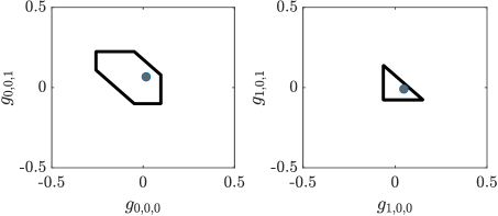
(b) Unique optimizer at boundary of $\Delta_{P}$

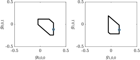
(c) $\arg\max_{Q\in\Delta_{P}}H_{Q}(T|XY)$ given by a line segment

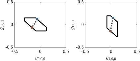
Figure 1. Three examples of $\Delta_{P}$ and $\arg\max_{Q\in\Delta_{P}}H_{Q}(T|XY)$ for $|\mathcal{T}|=2$,$|\mathcal{X}|=2$,$|\mathcal{Y}|=3$. Left plots show $\Delta_{P,0}$, while $\Delta_{P,1}$ is shown on the right side. Boundaries of $\Delta_{P}$ are marked by black lines, $\arg\max_{Q\in\Delta_{P}}H_{Q}(T|XY)$ is marked in gray. (a) There exists a unique optimizer in the interior of $\Delta_{P}$. (b) The unique optimizer lies at the boundary of $\Delta_{P}$. Note that both projections of the optimizer lies at the boundary of $\Delta_{P,0},\Delta_{P,1}$. (c) Gray lines mark the projections of $\arg\max_{Q\in\Delta_{P}}H_{Q}(T|XY)$ to $\Delta_{P,0}$ and $\Delta_{P,1}$.

5. The all binary case

If $X$, $Y$ and $T$ are all binary, $\Delta_{\mathcal{T},\mathcal{X},\mathcal{Y}}$ has 7 dimensions, which split in 5 dimensions for $V$ and 2 dimensions for $\Delta_{P}$. In this case it is possible to explicitly describe $\arg\max_{Q\in\Delta_{P}}H_{Q}(T|X,Y)$. This description will be developped throughout this chapter and summarized at the end of this section in Theorem 5.5.

Throughought this section we assume that $\mathcal{T}^{\prime}=\{0,1\}=\mathcal{X}=\mathcal{Y}$. In the following, $V$ is parameterized by the variables

(8) $$a=P_{T}(0), \begin{aligned} b=P_{X|T}(0|0),\\ c=P_{X|T}(0|1),\end{aligned} \begin{aligned} d=P_{Y|T}(0|0),\\ e=P_{Y|T}(0|1),\end{aligned}$$

and by the coefficients $g_{1},g_{2}$ of $a\gamma_{0;0,1;0,1},(1-a)\gamma_{1;0,1;0,1}$. Table 1 makes the parametrization (5) explicit.

$T$	$X$	$Y$	$P(t,x,y)$
0	0	0	$a(bd+g_{1})$
0	0	1	$a(b(1-d)-g_{1})$
0	1	0	$a((1-b)d-g_{1})$
0	1	1	$a((1-b)(1-d)+g_{1})$
1	0	0	$(1-a)(ce+g_{2})$
1	0	1	$(1-a)(c(1-e)-g_{2})$
1	1	0	$(1-a)((1-c)e-g_{2})$
1	1	1	$(1-a)((1-c)(1-e)+g_{2})$

Table 1. Parameterization of $2\times 2\times 2$ distributions

$\Delta_{P}$ is a rectangle. The allowed parameter domain is

$$-\min{\{bd,(1-b)(1-d)\}} \leq g_{1}\leq\min{\{b(1-d),(1-b)d\}}$$

$$-\min{\{ce,(1-c)(1-e)\}} \leq g_{2}\leq\min{\{c(1-e),(1-c)e\}}\text{ .}$$

The lower and upper bounds on $g_{i}$ will be denoted by $g_{i_{\min}}$ and $g_{i_{\max}}$ respectively.

The following holds:

1. $\Delta_{p,0}$ is a singleton iff $b\in\{0,1\}$ or $d\in\{0,1\}$.

2. $\Delta_{p,1}$ is a singleton iff $c\in\{0,1\}$ or $e\in\{0,1\}$.

3. $\Delta_{P}$ is a singleton iff both conditions are met. Thus, $\Delta_{P}$ degenerates to a single point precisely in the following four cases:

   1. $H(X|T)=0$;

   2. $H(Y|T)=0$;

   3. $H(X|T=0)=0$ and $H(Y|T=1)=0$;

   4. $H(X|T=1)=0$ and $H(Y|T=0)=0$.

In the all-binary case, Theorem 4.1 slightly generalizes:

Theorem 5.1.

Let $X,Y,T$ be binary. Suppose that ${\Delta}_{P}$ is not a singleton in case (c) or (d). If $\tilde{Q}=\arg\max_{Q\in\Delta_{P}}{H_{Q}(T|X,Y)}\in\overset{\circ}{\Delta}_{P}$, then $\left.T\mathchoice{\mathrel{\hbox to0.0pt{$\displaystyle\perp$\hss}\mkern 2.0mu{\displaystyle\perp}}}{\mathrel{\hbox to0.0pt{$\textstyle\perp$\hss}\mkern 2.0mu{\textstyle\perp}}}{\mathrel{\hbox to0.0pt{$\scriptstyle\perp$\hss}\mkern 2.0mu{\scriptstyle\perp}}}{\mathrel{\hbox to0.0pt{$\scriptscriptstyle\perp$\hss}\mkern 2.0mu{\scriptscriptstyle\perp}}}\!\!_{\smash{\tilde{Q}}}\;X\,\middle|\,Y\right.{}$ or $\left.T\mathchoice{\mathrel{\hbox to0.0pt{$\displaystyle\perp$\hss}\mkern 2.0mu{\displaystyle\perp}}}{\mathrel{\hbox to0.0pt{$\textstyle\perp$\hss}\mkern 2.0mu{\textstyle\perp}}}{\mathrel{\hbox to0.0pt{$\scriptstyle\perp$\hss}\mkern 2.0mu{\scriptstyle\perp}}}{\mathrel{\hbox to0.0pt{$\scriptscriptstyle\perp$\hss}\mkern 2.0mu{\scriptscriptstyle\perp}}}\!\!_{\smash{\tilde{Q}}}\;Y\,\middle|\,X\right.{}$.

Remark 5.2.

Example 6.4 shows that the conclusion does not in general hold in the singleton cases (c) and (d).

Proof.

The singleton cases (a) and (b) are trivial, and the remaining cases follow from Theorem 4.7. ∎

In the all-binary case, uniqueness can be completely characterized:

Theorem 5.3.

$\arg\max_{Q\in\Delta_{P}}{H_{Q}(T|X,Y)}$ is unique, unless $b=c$ and $d=e$.

Proof.

If $\arg\max_{Q\in\Delta_{P}}{H_{Q}(T|X,Y)}$ is not unique, then $\arg\max_{Q\in\overset{\circ}{\Delta}_{P}}{H_{Q}(T|X,Y)}$ is not unique either (by Lemma 3.3), so we may restrict attention to maximizers in the interior of $\Delta_{P}$. Thus, we assume that $b,c,d,e\notin\{0,1\}$.

First assume that $\Delta_{P}$ has full support. As shown in Theorem 4.1 and its proof, there are two cases $I$ and $I\!I$ to consider. Inserting the parameterization from above and using the injectivity of $\frac{1}{1+x}$ leads for case $I$ to the equations

$$\frac{ce+g_{2}}{bd+g_{1}} =\frac{(1-c)e-g_{2}}{(1-b)d-g_{1}}$$

$$\frac{c(1-e)-g_{2}}{b(1-d)-g_{1}} =\frac{(1-c)(1-e)+g_{2}}{(1-b)(1-d)+g_{1}}\text{ ,}$$

which simplify to

$$g_{2}d-g_{1}e =de(b-c)$$

$$g_{1}(1-e)-g_{2}(1-d) =(1-d)(1-e)(b-c)\text{ .}$$

Rearranging for $g_{1},g_{2}$ leads to

(9) $$g_{1}(d-e) =d(b-c)(1-d)$$

$$g_{2}(d-e) =e(b-c)(1-e)\text{ .}$$

For $d\neq e$, there exists a unique solution, and for $b=c$, the optimum is $Q_{0}$ itself. For $d=e$, there only exists a solution if $b=c$.

Similarly, case $I\!I$ reduces to

$$g_{2}b-g_{1}c =bc(d-e)$$

$$g_{1}(1-c)-g_{2}(1-b) =(1-b)(1-c)(d-e)$$

and rearranging for $g_{1},g_{2}$ gives

(10) $$g_{1}(b-c) =b(d-e)(1-b)$$

$$g_{2}(b-c) =c(d-e)(1-c)\text{ .}$$

Again, there exists a unique solution for $b\neq c$ and $Q_{0}$ is the optimum for $d=e$.

Now assume that $\Delta_{P}$ is a line. Following the proof of Theorem 5.1, assume that $b=0$. Plugging the parametrization from above into the equality $Q(1|10)=Q(1|11)$ gives

$$\frac{(1-a)\big{(}(1-c)e-g_{2}\big{)}}{(1-a)\big{(}(1-c)e-g_{2}\big{)}+P(010)}=\frac{(1-a)\big{(}(1-c)(1-e)+g_{2}\big{)}}{(1-a)\big{(}(1-c)(1-e)+g_{2}\big{)}+P(011)}.$$

If $P(010)=0$, then $P(011)=0$, and conversely; otherwise, this equation has no solution. In this case $P(010)=P(011)=0$, the sum $P(01)=P(010)+P(011)=a$ vanishes, which contradicts $\mathcal{T}^{\prime}=\{0,1\}$. Thus, $P(010)\neq 0$ and $P(011)\neq 0$. Using injectivity of $x\mapsto\frac{1}{1+x}$ and cancelling $(1-a)$, this is equivalent to

(11) $$\frac{(1-c)e-g_{2}}{P(010)}=\frac{(1-c)(1-e)+g_{2}}{P(011)}.$$

This equation is linear in $g_{2}$ and has a single unique solution, since the coefficient $\frac{1}{P(010)}+\frac{1}{P(011)}$ in front of $g_{2}$ is positive. ∎

Only the case where the maximizer lies on the boundary of $\Delta_{P}$ remains to be analyzed.

Theorem 5.4.

Assume that $\tilde{Q}=\arg\max_{Q\in\Delta_{P}}{H_{Q}(T|X,Y)}$ lies at the boundary of $\Delta_{P}$. Then, it is attained either at $(g_{1_{\min}},g_{2_{\min}})$ or $(g_{1_{\max}},g_{2_{\max}})$.

Proof.

If $\Delta_{P}$ is degenerate, then either $g_{1_{\min}}=g_{1_{\max}}$ or $g_{2_{\min}}=g_{2_{\max}}$, and the theorem becomes trivial. Otherwise, the statement follows from Lemma 3.3. ∎

The following theorem sums up the different possibilities.

Theorem 5.5.

For non-constant binary random variables $X$, $Y$ and $T$, there are five cases:

1. $b=c$ and $d=e$. In this case, $\left.X\mathchoice{\mathrel{\hbox to0.0pt{$\displaystyle\perp$\hss}\mkern 2.0mu{\displaystyle\perp}}}{\mathrel{\hbox to0.0pt{$\textstyle\perp$\hss}\mkern 2.0mu{\textstyle\perp}}}{\mathrel{\hbox to0.0pt{$\scriptstyle\perp$\hss}\mkern 2.0mu{\scriptstyle\perp}}}{\mathrel{\hbox to0.0pt{$\scriptscriptstyle\perp$\hss}\mkern 2.0mu{\scriptscriptstyle\perp}}}\!\!_{\smash{}}\;Y\,\middle|\,T\right.{}$ and $\arg\max_{Q\in\Delta_{P}}H_{Q}(T|X,Y)$ is not unique, but consists of the diagonal of $\Delta_{P}$.

2. $\left.T\mathchoice{\mathrel{\hbox to0.0pt{$\displaystyle\perp$\hss}\mkern 2.0mu{\displaystyle\perp}}}{\mathrel{\hbox to0.0pt{$\textstyle\perp$\hss}\mkern 2.0mu{\textstyle\perp}}}{\mathrel{\hbox to0.0pt{$\scriptstyle\perp$\hss}\mkern 2.0mu{\scriptstyle\perp}}}{\mathrel{\hbox to0.0pt{$\scriptscriptstyle\perp$\hss}\mkern 2.0mu{\scriptscriptstyle\perp}}}\!\!_{\smash{\tilde{Q}}}\;X\,\middle|\,Y\right.{}$ for the unique $\tilde{Q}=\arg\max_{Q\in\Delta_{P}}H_{Q}(T|X,Y)$.

3. $\left.T\mathchoice{\mathrel{\hbox to0.0pt{$\displaystyle\perp$\hss}\mkern 2.0mu{\displaystyle\perp}}}{\mathrel{\hbox to0.0pt{$\textstyle\perp$\hss}\mkern 2.0mu{\textstyle\perp}}}{\mathrel{\hbox to0.0pt{$\scriptstyle\perp$\hss}\mkern 2.0mu{\scriptstyle\perp}}}{\mathrel{\hbox to0.0pt{$\scriptscriptstyle\perp$\hss}\mkern 2.0mu{\scriptscriptstyle\perp}}}\!\!_{\smash{\tilde{Q}}}\;Y\,\middle|\,X\right.{}$ for the unique $\tilde{Q}=\arg\max_{Q\in\Delta_{P}}H_{Q}(T|X,Y)$.

4. The unique maximizer lies at $(g_{1_{\min}},g_{2_{\min}})$.

5. The unique maximizer lies at $(g_{1_{\max}},g_{2_{\max}})$.

Remark 5.6.

(1) The last four cases in Theorem 5.5 intersect. For example, the intersection of the last four cases contains the distribution $\frac{1}{2}\delta_{000}+\frac{1}{2}\delta_{111}$ (see [6, 14] for a discussion of the intersection of cases (2) and (3)).

(2) In cases 2. and 3., if $0<b,c,d,e<1$, then $\tilde{Q}$ can be computed by solving (9) or (10). If $b=0$, then $\tilde{Q}$ can be computed in cases 2. and 3. by solving (11). Similar equations can be obtained if $b=1$ or if any of $c,d,e$ lies in $\{0,1\}$.

(3) The five cases can be distinguished by polynomial inequalities among the parameters $a,b,c,d,e$. Therefore, the five cases correspond to five semi-algebraic sets of probability distributions. For example, case (2) holds if and only if the unique solution $(g_{1},g_{2})$ to (9) satisfies $g_{i_{\min}}\leq g_{i}\leq g_{i_{\max}}$ for $i=1,2$, which can be formulated as eight polynomial inequalities.

6. Examples

Example 6.1 (For ternary $T$, maximizers with full support need not satisfy CI statements).

Let $X,Y$ be binary random variables with $P(X,Y)$ arbitrary (of full support), and let $T$ be ternary with

$$(P(T=1|X=x,Y=y))_{x,y} =\begin{pmatrix}\frac{1}{3}&\frac{1}{2}\\ \frac{1}{12}&\frac{1}{8}\end{pmatrix},$$

$$(P(T=2|X=x,Y=y))_{x,y} =\begin{pmatrix}\frac{1}{3}&\frac{1}{8}\\ \frac{5}{24}&\frac{5}{64}\end{pmatrix},$$

$$(P(T=3|X=x,Y=y))_{x,y} =\begin{pmatrix}\frac{1}{3}&\frac{3}{8}\\ \frac{17}{24}&\frac{51}{64}\end{pmatrix}$$

Then $P$ minimizes $I_{Q}(T:X|Y)$ on $\Delta_{P}$ (cf. Remark 3.2), and one can check that $P$ is the unique minimizer on $\Delta_{P}$ (it is impossible to find a line through $P$ in $\Delta_{P}$ such that the two points at which this line hits the boundary satisfy the conclusion of Lemma 3.3). $P$ has full support, but there is no conditional independence statement.

Example 6.2 (An illustration of Theorem 3.10).

Consider the distributions

$x$	$y$	$t$	$P(x,y,t)$
0	0	0	$\tfrac{1}{6}$
0	0	1	$\tfrac{1}{6}$
1	1	0	$\tfrac{1}{6}$
1	1	1	$\tfrac{1}{6}$
2	2	0	$\tfrac{1}{9}$
2	2	1	$\tfrac{2}{9}$

$x$	$y$	$t$	$P^{\prime}(x,y,t)$
0	1	0	$\tfrac{1}{6}$
0	1	1	$\tfrac{1}{6}$
1	0	0	$\tfrac{1}{6}$
1	0	1	$\tfrac{1}{6}$
2	2	0	$\tfrac{1}{9}$
2	2	1	$\tfrac{2}{9}$

Then $\left.T\mathchoice{\mathrel{\hbox to0.0pt{$\displaystyle\perp$\hss}\mkern 2.0mu{\displaystyle\perp}}}{\mathrel{\hbox to0.0pt{$\textstyle\perp$\hss}\mkern 2.0mu{\textstyle\perp}}}{\mathrel{\hbox to0.0pt{$\scriptstyle\perp$\hss}\mkern 2.0mu{\scriptstyle\perp}}}{\mathrel{\hbox to0.0pt{$\scriptscriptstyle\perp$\hss}\mkern 2.0mu{\scriptscriptstyle\perp}}}\!\!_{\smash{P}}\;Y\,\middle|\,X\right.{}$ and $\left.T\mathchoice{\mathrel{\hbox to0.0pt{$\displaystyle\perp$\hss}\mkern 2.0mu{\displaystyle\perp}}}{\mathrel{\hbox to0.0pt{$\textstyle\perp$\hss}\mkern 2.0mu{\textstyle\perp}}}{\mathrel{\hbox to0.0pt{$\scriptstyle\perp$\hss}\mkern 2.0mu{\scriptstyle\perp}}}{\mathrel{\hbox to0.0pt{$\scriptscriptstyle\perp$\hss}\mkern 2.0mu{\scriptscriptstyle\perp}}}\!\!_{\smash{P^{\prime}}}\;Y\,\middle|\,X\right.{}$ as well as $\left.T\mathchoice{\mathrel{\hbox to0.0pt{$\displaystyle\perp$\hss}\mkern 2.0mu{\displaystyle\perp}}}{\mathrel{\hbox to0.0pt{$\textstyle\perp$\hss}\mkern 2.0mu{\textstyle\perp}}}{\mathrel{\hbox to0.0pt{$\scriptstyle\perp$\hss}\mkern 2.0mu{\scriptstyle\perp}}}{\mathrel{\hbox to0.0pt{$\scriptscriptstyle\perp$\hss}\mkern 2.0mu{\scriptscriptstyle\perp}}}\!\!_{\smash{P}}\;X\,\middle|\,Y\right.{}$ and $\left.T\mathchoice{\mathrel{\hbox to0.0pt{$\displaystyle\perp$\hss}\mkern 2.0mu{\displaystyle\perp}}}{\mathrel{\hbox to0.0pt{$\textstyle\perp$\hss}\mkern 2.0mu{\textstyle\perp}}}{\mathrel{\hbox to0.0pt{$\scriptstyle\perp$\hss}\mkern 2.0mu{\scriptstyle\perp}}}{\mathrel{\hbox to0.0pt{$\scriptscriptstyle\perp$\hss}\mkern 2.0mu{\scriptscriptstyle\perp}}}\!\!_{\smash{P^{\prime}}}\;X\,\middle|\,Y\right.{}$, and $P^{\prime}\in\Delta_{P}$. It follows that $I_{P}(T:Y|X)=I_{P^{\prime}}(T:Y|X)=0$, whence $P$ and $P^{\prime}$ are both minimizers. The same holds true for any convex combination of $P$ and $P^{\prime}$. Note that $P$ and $P^{\prime}$ (more generally: any convex combination of $P$ and $P^{\prime}$) have restricted support: the probability of $\big{\{}X=2,Y\neq 2\big{\}}$ vanishes. On the other hand, $\operatorname{supp}(\Delta_{P})$ is full.

Example 6.3 (The all-binary case where $\Delta_{P}$ is a line).

Consider the $2\times 2\times 2$ distribution given by $e=0$ and $a,b,c,d=\tfrac{1}{2}$

$T$	$X$	$Y$	$P(t,x,y)$
0	0	0	$\tfrac{1}{8}$
0	0	1	$\tfrac{1}{8}$
0	1	0	$\tfrac{1}{8}$
0	1	1	$\tfrac{1}{8}$
1	0	1	$\tfrac{1}{4}$
1	1	1	$\tfrac{1}{4}$

$\Delta_{P}$ degenerates to a line $P+g_{1}\gamma_{0;0,1;0,1}$ with support $-\tfrac{1}{8}\leq g_{1}\leq\tfrac{1}{8}$. The conditional entropy is

$$H_{g_{1}}(T|X,Y) =(\tfrac{3}{8}-g_{1})H_{g_{1}}(T|0,1)+(\tfrac{3}{8}+g_{1})H_{g_{1}}(T|1,1)$$

$$=(\tfrac{3}{8}-g_{1})h\bigg{(}\frac{\tfrac{1}{8}-g_{1}}{\tfrac{3}{8}-g_{1}},\frac{\tfrac{1}{4}}{\tfrac{3}{8}-g_{1}}\bigg{)}+(\tfrac{3}{8}+g_{1})h\bigg{(}\frac{\tfrac{1}{8}+g_{1}}{\tfrac{3}{8}+g_{1}},\frac{\tfrac{1}{4}}{\tfrac{3}{8}+g_{1}}\bigg{)}.$$

By symmetry and Lemma 3.5, the unique maximizer of $H_{g_{1}}(T|X,Y)$ lies at $g_{1}=0$, that is, $P$ is the unique solution to the optimization problem. In this case, $P$ equals $Q_{0}$; that is, $\left.X\mathchoice{\mathrel{\hbox to0.0pt{$\displaystyle\perp$\hss}\mkern 2.0mu{\displaystyle\perp}}}{\mathrel{\hbox to0.0pt{$\textstyle\perp$\hss}\mkern 2.0mu{\textstyle\perp}}}{\mathrel{\hbox to0.0pt{$\scriptstyle\perp$\hss}\mkern 2.0mu{\scriptstyle\perp}}}{\mathrel{\hbox to0.0pt{$\scriptscriptstyle\perp$\hss}\mkern 2.0mu{\scriptscriptstyle\perp}}}\!\!_{\smash{P}}\;Y\,\middle|\,T\right.{}$ holds. Moreover, $\left.T\mathchoice{\mathrel{\hbox to0.0pt{$\displaystyle\perp$\hss}\mkern 2.0mu{\displaystyle\perp}}}{\mathrel{\hbox to0.0pt{$\textstyle\perp$\hss}\mkern 2.0mu{\textstyle\perp}}}{\mathrel{\hbox to0.0pt{$\scriptstyle\perp$\hss}\mkern 2.0mu{\scriptstyle\perp}}}{\mathrel{\hbox to0.0pt{$\scriptscriptstyle\perp$\hss}\mkern 2.0mu{\scriptscriptstyle\perp}}}\!\!_{\smash{P}}\;X\,\middle|\,Y\right.{}$ holds.

Example 6.4 (The all-binary case where $\Delta_{P}$ is a singleton).

Consider the $2\times 2\times 2$ distribution given by $b=e=1$ and $a,c,d=\tfrac{1}{2}$:

$T$	$X$	$Y$	$P(t,x,y)$
0	0	0	$\tfrac{1}{4}$
0	0	1	$\tfrac{1}{4}$
1	0	0	$\tfrac{1}{4}$
1	1	0	$\tfrac{1}{4}$

Here, $\Delta_{P}$ is a singleton. Neither $\left.T\mathchoice{\mathrel{\hbox to0.0pt{$\displaystyle\perp$\hss}\mkern 2.0mu{\displaystyle\perp}}}{\mathrel{\hbox to0.0pt{$\textstyle\perp$\hss}\mkern 2.0mu{\textstyle\perp}}}{\mathrel{\hbox to0.0pt{$\scriptstyle\perp$\hss}\mkern 2.0mu{\scriptstyle\perp}}}{\mathrel{\hbox to0.0pt{$\scriptscriptstyle\perp$\hss}\mkern 2.0mu{\scriptscriptstyle\perp}}}\!\!_{\smash{P}}\;Y\,\middle|\,X\right.{}$ nor $\left.T\mathchoice{\mathrel{\hbox to0.0pt{$\displaystyle\perp$\hss}\mkern 2.0mu{\displaystyle\perp}}}{\mathrel{\hbox to0.0pt{$\textstyle\perp$\hss}\mkern 2.0mu{\textstyle\perp}}}{\mathrel{\hbox to0.0pt{$\scriptstyle\perp$\hss}\mkern 2.0mu{\scriptstyle\perp}}}{\mathrel{\hbox to0.0pt{$\scriptscriptstyle\perp$\hss}\mkern 2.0mu{\scriptscriptstyle\perp}}}\!\!_{\smash{P}}\;X\,\middle|\,Y\right.{}$ holds.

7. Conclusions

In this work we investigated uniqueness and support of the solutions to the optimization problem underlying the definition of the unique information function $UI(T:X\setminus Y)$ defined by Bertschinger et al. [4]. This optimization problem consists of maximizing the conditional entropy $H(T|XY)$ over the space of probability distributions with fixed pairwise $TX,TY$ marginals. We showed that this conditional entropy is not strictly concave in exactly the directions in which $P(T|XY)$ is constant. From this we showed that all optima that are attained in the interior of the optimization space which have full support are not unique if $|\mathcal{T}|<\max(|\mathcal{X}|,|\mathcal{Y}|)$ and identified sufficient conditions for non-uniqueness that relate to independence statements. If the variable $\mathcal{T}$ is binary we showed partial converses of these results. In this case, vanishing of the directional derivatives of the $H(T|XY)$ implies a conditional independence $\left.T\mathchoice{\mathrel{\hbox to0.0pt{$\displaystyle\perp$\hss}\mkern 2.0mu{\displaystyle\perp}}}{\mathrel{\hbox to0.0pt{$\textstyle\perp$\hss}\mkern 2.0mu{\textstyle\perp}}}{\mathrel{\hbox to0.0pt{$\scriptstyle\perp$\hss}\mkern 2.0mu{\scriptstyle\perp}}}{\mathrel{\hbox to0.0pt{$\scriptscriptstyle\perp$\hss}\mkern 2.0mu{\scriptscriptstyle\perp}}}\!\!_{\smash{}}\;Y\,\middle|\,X\right.{}$ or $\left.T\mathchoice{\mathrel{\hbox to0.0pt{$\displaystyle\perp$\hss}\mkern 2.0mu{\displaystyle\perp}}}{\mathrel{\hbox to0.0pt{$\textstyle\perp$\hss}\mkern 2.0mu{\textstyle\perp}}}{\mathrel{\hbox to0.0pt{$\scriptstyle\perp$\hss}\mkern 2.0mu{\scriptstyle\perp}}}{\mathrel{\hbox to0.0pt{$\scriptscriptstyle\perp$\hss}\mkern 2.0mu{\scriptscriptstyle\perp}}}\!\!_{\smash{}}\;X\,\middle|\,Y\right.{}$ and thus vanishing of the corresponding unique informations. Imposing such an independence relation on the optimization domain led to a set of linear constraints. Thus, by solving this linear problems we solve the optimization problem if there exists a solution in the interior, otherwise we reduce the optimization domain to its boundary. Numerical experiments showed that a noticeable fraction of distributions sampled uniformely from the probability simplex have corresponding optima in the interior. This fraction becomes smaller with growing cardinalities of $|\mathcal{X}|,|\mathcal{Y}|$. We derived an analytical solution of the optimization problem when all variables are binary. Whenever possible, we gave extensions to the theorems relaxing the assumptions on the support of the optima and gave examples showing that the assumptions in our theorems are neccesary.

Authors’ Contributions

Work on this project was initiated by questions of JJ. Initial results for the all binary case were obtained by MS and JJ. MS and JR worked together to generalize and complete the results. MS and JR wrote the paper. All authors read and approved the final manuscript.

References

• Amari and Nagaoka [2000] Shun-ichi Amari and Hiroshi Nagaoka. Methods of Information Geometry, volume 191 of Translations of mathematical Monographs. American Mathematical Society, first edition, 2000.
• Banerjee et al. [2018a] Pradeep Kr. Banerjee, Eckehard Olbrich, Jürgen Jost, and Johannes Rauh. Unique informations and deficiencies. In Proceedings of Allerton, 2018a.
• Banerjee et al. [2018b] Pradeep Kr. Banerjee, Johannes Rauh, and Guido Montúfar. Computing the unique information. In Proc. IEEE ISIT, pages 141–145. IEEE, 2018b.
• Bertschinger et al. [2014] Nils Bertschinger, Johannes Rauh, Eckehard Olbrich, Jürgen Jost, and Nihat Ay. Quantifying unique information. Entropy, 16(4):2161–2183, 2014.
• Diaconis and Sturmfels [1998] Persi Diaconis and Bernd Sturmfels. Algebraic algorithms for sampling from conditional distributions. Annals of Statistics, 26:363–397, 1998.
• Fink [2011] Alex Fink. The binomial ideal of the intersection axiom for conditional probabilities. Journal of Algebraic Combinatorics, 33(3):455–463, 2011.
• Finn and Lizier [2018] Conor Finn and Joseph T. Lizier. Pointwise partial information decomposition using the specificity and ambiguity lattices. Entropy, 20(4):297, 2018.
• Harder et al. [2013] Malte Harder, Christoph Salge, and Daniel Polani. A bivariate measure of redundant information. Phys. Rev. E, 87:012130, Jan 2013.
• Ince [2017] Robin Ince. Measuring multivariate redundant information with pointwise common change in surprisal. Entropy, 19(7):318, 2017.
• James et al. [2018] Ryan James, Jeffrey Emenheiser, and James Crutchfield. Unique information via dependency constraints. Journal of Physics A, 52(1):014002, 2018.
• Makkeh et al. [2017] Abdullah Makkeh, Dirk Oliver Theis, and Raul Vicente. Bivariate partial information decomposition: The optimization perspective. Entropy, 19(10):530, 2017.
• Niu and Quinn [2019] Xueyan Niu and Christopher Quinn. A measure of synergy, redundancy, and unique information using information geometry. In Proc. IEEE ISIT, 2019.
• Rauh et al. [2019] J. Rauh, P. Kr. Banerjee, E. Olbrich, and J. Jost. Unique information and secret key decompositions. In 2019 IEEE International Symposium on Information Theory (ISIT), pages 3042–3046, 2019.
• Rauh and Ay [2014] Johannes Rauh and Nihat Ay. Robustness, canalyzing functions and systems design. Theory in Biosciences, 133(2):63–78, 2014.
• Rauh et al. [2014] Johannes Rauh, Nils Bertschinger, Eckehard Olbrich, and Jürgen Jost. Reconsidering unique information: Towards a multivariate information decomposition. In Proc. IEEE ISIT, pages 2232–2236, 2014.
• Smith and Tromble [2004] Noah A Smith and Roy W Tromble. Sampling uniformly from the unit simplex. Johns Hopkins University, Tech. Rep, 29, 2004.
• Williams and Beer [2010] Paul Williams and Randall Beer. Nonnegative decomposition of multivariate information. arXiv:1004.2515v1, 2010.