Quantum critical scaling of gapped phases in nodal-line semimetals

Abstract

We study the effect of short range interactions in three dimensional nodal-line semimetals with linear band crossings. We analyze the Yukawa theories for gapped instabilities in the charge, spin and superconducting channels using the Wilsonian renormalization group framework, employing a large number of fermion flavors $N_{f}$ for analytical control. We obtain stable non-trivial fixed points and provide a unified description of the critical exponents for the ordering transitions in terms of the number of order parameter components $N_{b}$ systematically to order $1/N_{f}$. We show that in all cases, the dynamical exponent $z=1$ in one loop, whereas $1/N_{f}$ corrections to various exponents follow from the anomalous dimension of the bosonic fields only.

I Introduction

Three dimensional (3D) nodal-line semimetals describe an interesting class of fermionic systems where the valence and conduction bands touch along manifolds of codimension $d_{c}=2$. Rather than forming around points, such as in graphene Neto or in Dirac and Weyl semimetals Wan-1 ; Armitage , the quasiparticles can appear around closed lines in the 3D Brillouin zone, which are protected by symmetries of the Hamiltonian Fang ; Yang-sym ; Chan-sym ; Wang-sym ; Chiu-1 . Nodal-line semimetals have been originally predicted in a variety of different contexts Arovas ; Heikkila ; Burkov ; Xu ; Mullen ; Weng2 ; Kim ; Weng and were more recently observed in different materials Xie ; Bian ; Bian2 ; Yan ; Fu ; Deng , in photonic crystals Lu and also in cold atom systems Song .

In general, electron-electron interactions open up a myriad of new possibilities for non-Fermi liquid behavior and various broken symmetry phases in materials with nodal points or lines. Long range Coulomb interactions in Dirac and Weyl semimetals have been shown to be isotropic, marginal and lead to logarithmic corrections to physical quantities at low energies Kotov ; Sekine ; Goswami ; Hosur ; Throckmorton ; Gonsalez . In anisotropic systems, Coulomb interactions may lead to non-Fermi liquid behavior over a wide range of energy scales Isobe ; Moon ; Herbut , or else be irrelevant in the perturbative regime Huh ; Wang-1 ; Yang-1 . Short-range interactions, on the other hand, can lead to continuous quantum phase transitions resulting in spontaneously ordered phases. For instance, in the case of Dirac fermions in the honeycomb lattice, the critical behavior was shown to belong to the Gross-Neveu-Yukawa universality class Herbut-1 ; Assad . 2D semi-Dirac fermions, which exist at a topological phase transition between a semimetallic and a gapped phase, where two Dirac cones merge Montambaux , have unconventional quantum criticality Uryszek ; Roy ; Sur . They show correlation lengths that diverge along different directions with distinct exponents, which may result in novel exotic superconductivity with smectic order Uchoa . In Weyl semimetals, short range interactions lead either to a first-order phase transition into a band insulator or else to a continuous transition into a symmetry breaking phase Roy-1 .

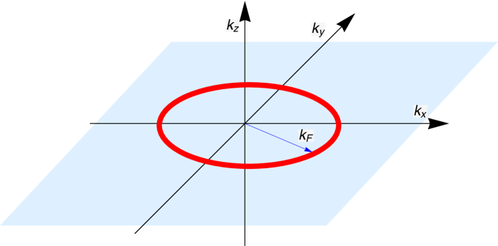
Figure 1: Ring of nodal points in the $k_{z}=0$ plane resulting from the spectrum of the free Hamiltonian (2). The light blue shaded region represents the plane of the nodal line. Nodal loop of radius $k_{F}$ is shown in red.

We contribute to this endeavor by investigating the effect of short-range interactions on 3D nodal-line semimetals with linear band crossings. We address the relatively general case where the nodal line forms a closed ring or loop centered at the 3D Brillouin zone, as depicted in Fig. 1. Due to the vanishing density of states at the nodal line, the expected many-body instabilities occur through a quantum phase transition separating the semimetallic regime from spontaneously broken symmetry phases Nandikshore ; Roy-2 . We investigate the universal quantum critical scaling for instabilities in the spin, charge and superconducting channels that produce fully gapped states.

Using a Wilson momentum shell renormalization group (RG) in the Yukawa language, we analyze the interacting fixed points for the different channels. We augment the action with a large number of fermionic flavors $N_{f}$ for analytical control and derive their corresponding critical exponents in leading $1/N_{f}$ order. In one loop, we show that the mean field results are exact in the $s$-wave superconducting (SC) channel, where vertex corrections vanish, whereas in both the charge density wave (CDW) and spin density wave (SDW) orders we obtain finite $1/N_{f}$ corrections. In all cases, the dynamical exponent

$$z=1+O(N_{f}^{-2})$$ (1)

in the regime where the radius of the nodal line is large compared to all other energy scales. The critical exponents are summarized in a table, which is the main result of the paper.

As the outline of the paper, we introduce the Yukawa action of the problem in section II. In section III, we discuss the Wilson RG scheme for nodal-line semimetals, where we derive the RG equations for contact interactions in the various channels. We then calculate the fixed points and their respective critical exponents to leading order in $1/N_{f}$. Finally, in section IV we present our conclusions.

II MODEL

We consider the simplest non-interacting low energy Hamiltonian for a nodal-line semimetal, which supports an isolated closed circular loop of Fermi points with radius $k_{F}$. The nodal line is centered around the origin of the Brillouin zone in the $k_{x}-k_{y}$ plane,

$$\mathcal{H}_{0}=\frac{k_{x}^{2}+k_{y}^{2}-k_{F}^{2}}{2m}\tau_{0}\otimes\sigma_{y}+v_{z}k_{z}\tau_{0}\otimes\sigma_{x},$$ (2)

where $\tau_{i}$ and $\sigma_{i}$ are Pauli matrices acting on the spin and orbital/sublattice degrees of freedom. The four-component spinor basis is defined as $\psi_{k}^{T}\equiv\left(\varphi_{1,\uparrow,\mathbf{k}},\varphi_{2,\uparrow,\mathbf{k}},\varphi_{1,\downarrow,\mathbf{k}},\varphi_{2,\mathbf{\downarrow,}\mathbf{k}}\right)$, where $1,2$ denote pseudospin and $\uparrow,\downarrow$ spin quantum numbers. Lattice realizations of this model have been proposed in different contexts, including hyperhoneycomb lattices Mullen , graphene networks Weng2 and cubic crystals Roy-2 . Near the nodal loop,

$$\frac{k_{x}^{2}+k_{y}^{2}-k_{F}^{2}}{2m}\simeq v_{r}\tilde{k}_{r}$$

where $\tilde{k}_{r}=\sqrt{k_{x}^{2}+k_{y}^{2}}-k_{F}$ and $v_{{}_{r}}=\frac{k_{F}}{m}$ is the radial Fermi velocity. Thus the quasiparticles disperse linearly in all directions that are normal to the nodal line. The action for the non interacting part is therefore given by

$$\mathcal{S}_{\psi}=\sum_{n=1}^{N_{f}}\int dk\ \bar{\psi}_{n,k}\left[-ik_{0}+\mathcal{H}_{0}\right]\psi_{n,k}$$ (3)

where $k=\left(k_{0},k_{x},k_{y},k_{z}\right)$ is the four-momentum vector in 3+1 dimensions, with $k_{0}$ the frequency and $\int dk\equiv(2\pi)^{-4}\int dk_{0}dk_{x}dk_{y}dk_{z}.$ $\psi_{n,k}$ represents the fermion field carrying a flavor index $n$, with $N_{f}$ the number of fermionic flavors, which are treated as a degeneracy.

To study the quantum critical behavior of the nodal-loop system, we use a Hubbard-Stratanovich decomposition of the four-fermion interaction into appropriate channels and study the resulting Gross-Neveau-Yukawa theories. Short range interactions can lead to mass terms of the form $\sum_{i=1}^{N_{b}}M_{i}\Gamma_{i}$, where $\Gamma_{i}$ are all possible $4\times 4$ matrices that anticommute with the noninteracting Hamiltonian (2). In this class of phase transitions, the mass term describes the spontaneous chiral symmetry breaking of the system across a quantum critical point into a gapped phase. The Yukawa coupling term in the action can then be generically written as

$$\mathcal{S}_{\phi\psi}=g\sum_{n=1}^{N_{f}}\sum_{j}^{N_{b}}\int dkdq\,\phi_{q}^{j}\left(\bar{\psi}_{n,k}\Gamma_{j}\psi_{n,k-q}\right)$$ (4)

where

$$\Gamma_{j}=\tau_{j}\otimes\sigma_{3},$$ (5)

with $j=0,1,2,3$ are the only four possible mass terms that lead to gapped phases in the considered Hilbert space.

CDW and SDW instabilities correspond to staggered patterns of charge and spin in the pseudospin space. The effective single particle interaction Hamiltonian that describes those instabilities is of the form

$$\mathcal{H}_{CDW}=\phi^{0}\tau_{0}\otimes\sigma_{3},$$ (6)

and

$$\mathcal{H}_{SDW}=\boldsymbol{\phi}\cdot\boldsymbol{\tau}\otimes\sigma_{3}$$ (7)

respectively, where $\boldsymbol{\phi}=\left(\phi^{1},\phi^{2},\phi^{3}\right)$ is a vector order parameter and $\boldsymbol{\tau}=\left(\tau_{1},\tau_{2},\tau_{3}\right)$. Clearly, these terms anticommute with the noninteracting Hamiltonian (2), leading to gaps in the spectrum. To identify the vertex of the $s$-wave superconducting case, it is convenient to double the size of the Hilbert space and introduce the 8-component Nambu spinor basis $\Psi_{k}^{T}=\left(\varphi_{1,\uparrow,\mathbf{k}},\varphi_{2,\uparrow,\mathbf{k}},\varphi_{1,\downarrow,\mathbf{k}},\varphi_{2,\mathbf{\downarrow,}\mathbf{k}},\varphi_{1,\downarrow,-\mathbf{k}}^{\dagger},\varphi_{2,\downarrow,-\mathbf{k}}^{\dagger},\varphi_{1,\uparrow,-\mathbf{k}}^{\dagger},\varphi_{2,\mathbf{\uparrow,}-\mathbf{k}}^{\dagger}\right)$. In this basis, the non-interacting part of the Hamiltonian can be written as

$$\mathcal{H}_{0}=\frac{k_{x}^{2}+k_{y}^{2}-k_{F}^{2}}{2m}\eta_{0}\otimes\tau_{0}\otimes\sigma_{y}+v_{z}k_{z}\eta_{0}\otimes\tau_{0}\otimes\sigma_{x},$$ (8)

where the Pauli matrices $\eta_{i}$ ($i=0,1,2,3$) act in the Nambu space. The fully gapped $s$-wave pairing term that anticommutes with (8) has the form $\mathcal{H}_{SC}=\boldsymbol{\phi}\cdot\boldsymbol{\eta}_{\perp}\otimes\tau_{0}\otimes\sigma_{3}$ where $\boldsymbol{\phi}=(\phi_{1},\phi_{2})$ is a vector whose components are defined in terms of the real and imaginary parts of the order parameter, and $\boldsymbol{\eta}_{\perp}=(\eta_{1},\eta_{2}).$ One can see that the spin space is redundant in this basis, as it corresponds to two identical $4\times 4$ copies of the Hamiltonian. Therefore, we drop for convenience the $\tau_{0}$ matrices in $\mathcal{H}_{0}$ and $\mathcal{H}_{SC}$ and absorb the spin as a degeneracy. In that case, the pairing term has the form

$$\mathcal{H}_{SC}=\boldsymbol{\phi}\cdot\boldsymbol{\eta}_{\perp}\otimes\sigma_{3}.$$ (9)

The Yukawa vertex that follows from this term has the same form of Eq. (5) for $j=1,2$ if one performs the substitution $\eta_{i}\leftrightarrow\tau_{i}$. As expected, the pairing term is dual to the antiferromagnetic XY model.

In all cases, we can identify the different mass terms that correspond to distinct channels of instabilities in the charge, spin and $s$-wave superconducting states with a Yukawa vertex of the form (5) written in some appropriate basis. The different ordered states encoded in the generic Yukawa coupling (5) are

$$j=\begin{cases}0&\text{CDW}\\ 1,2&\text{SC}\\ 1,2,3&\text{SDW}\end{cases}.$$ (10)

Here, $N_{b}=1,2$,$3$ describes respectively the number of bosonic field components in the CDW, SC and SDW cases, respectively.

Other possible emergent mass terms leading to fully gapped states are allowed if one enlarges the size of the Hilbert space. For instance, in 2D Dirac fermions on the honeycomb lattice, an anomalous quantum Hall (AQH) state is in principle allowed Raghu ; Christou when one reverses the sign of the mass term across opposite valleys. In nodal-line semimetals, where the concept of valleys is ill defined, the reversal of the sign of the mass in the AQH state happens continuously along the nodal line. Due to particle-hole symmetry, which keeps the mass purely imaginary and hence topological, this state does not produce a fully gapped state, but rather a Weyl semimetal, with Fermi arcs connecting a discrete number of gapless points of the nodal line, where the mass term changes sign Kim-Hall . Although this is an interesting state, it is highly dependent on the microscopic details of the lattice model, such as the number of nodes of the mass along the nodal line Kim-Hall ; Okugawa , and will be considered elsewhere. Here, we will restrict our analysis to isotropic instabilities in the considered Hilbert space that fully gap the nodal line.

The free part of the bosonic action can be written as

$$\mathcal{S}_{\phi}=\sum_{j=1}^{N_{b}}\int dq\phi_{-q}^{j}\left(c_{0}^{2}q_{0}^{2}+c_{1}^{2}(q_{x}^{2}+q_{y}^{2})+c_{2}^{2}q_{z}^{2}+m_{\phi}^{2}\right)\phi_{q}^{j},$$ (11)

in which we have also included the gradient terms that will be generated in the ultraviolet (UV) through the RG process. Therefore the action for the field theory describing the problem of interest is given by

$$\mathcal{S}=\mathcal{S}_{\psi}+\mathcal{S}_{\phi}+\mathcal{S}_{\phi\psi}.$$ (12)

We now proceed with the momentum shell RG accounting for both the fermionic and bosonic fields.

III RENORMALIZATION GROUP

In this section, we perform one loop RG calculations of the Yukawa action and derive the flow equations for various coupling constants in the action. As pointed out in Ref. Huh ; Wang-1 , the presence of the nodal ring requires that the fermionic and bosonic momenta be treated differently. While fermionic momenta should be rescaled towards to the nodal ring, bosonic momenta is rescaled towards the origin of momentum space. This has important implications for the tree level scaling analysis.

For fermionic momenta, we take the tree level scaling dimensions to be

$$\left[k_{0}\right]=z,\quad\left[\tilde{k}_{r}\right]=1,\quad\left[k_{z}\right]=z_{1},$$ (13)

where $z_{1}$ is introduced for computational convenience and will be set to unity later. The scaling dimension of the 3D fermionic integral $[\int\!dk]=2$ due to the fact that the radius of the nodal ring $k_{F}$ does not run Huh ; Wang-1 . Tree level scaling invariance of the fermionic part of the action hence requires that $\left[\psi\right]=-\frac{1}{2}(2z+z_{1}+1)$, setting the scaling dimensions of velocities as $\left[v_{r}\right]=z-1$ and $\left[v_{r}\right]=z-z_{1}$. For the bosonic part,

$$\left[q_{0}\right]=z,\quad\left[q_{x}\right]=\left[q_{y}\right]=\left[q_{z}\right]=1.$$

Since $[\int\!dq]=3$, this implies that the scaling dimension of the bosonic fields is $\left[\phi\right]=-\frac{3}{2}\left(z+1\right)$, whereas the coupling constants $c_{0}$, $c_{1}$ and $c_{2}$ remain marginal at the tree level. This saves us from unphysical infrared divergences of the bosonic propagator Uryszek . In our analysis, we assume that important contributions arise when momenta $q$ is small compared to the radius of the ring $k_{F}$, and hence correspond to processes with small momentum transfer near the nodal line. In that spirit, we ignore corrections of the order of $\sim$$|q|/k_{F}$, as is appropriate when the nodal loop has a large radius compared to all other energy scales.

To be consistent with this approximation, we have to ensure that one of the momenta ($q$) in Eq. 4 is bosonic, and the other ($k$) fermionic. With this, one can see that the Yukawa coupling has scaling dimensions

$$\left[g\right]=\frac{3}{2}\left(z-1\right),$$ (14)

and is therefore marginal at the tree level.

Different implementations of the momentum shell integration have been employed in the study of nodal-line semimetals. A cylindrical momentum shell integration scheme was used in Ref. Huh whereas a more symmetric mode elimination in a toroidal geometry was used in Ref. Sur-1 . With the understanding that physical quantities do not depend on the renormalization scheme, we employ a different one in which frequency and momenta are treated on the same footing. For fermionic momenta, we perform mode elimination by integrating out fast modes that lie in a thin shell around the nodal line,

$$\Lambda e^{-zd\ell}<\sqrt{k_{0}^{2}+E_{k}^{2}}<\Lambda,$$ (15)

where $E_{k}^{2}=v_{r}^{2}\tilde{k}_{r}^{2}+v_{z}^{2}k_{z}^{2}$.

For bosonic momenta, we integrate out modes that lie in a thin shell defined by

$$\Lambda e^{-zd\ell}<\sqrt{q_{0}^{2}+q_{x}^{2}+q_{y}^{2}+q_{z}^{2}}<\Lambda.$$ (16)

In either case, we assume that the UV energy cutoff $\Lambda$ is small compared to the radius of the nodal ring, $\Lambda/v_{r}k_{F}\ll 1$. Another important distinction that is specific to nodal-line semimetals is the fact that in keeping the radius of the nodal line $k_{F}$ fixed, the UV cut-off has a finite scaling dimension $[\Lambda]=-z$, which is incorporated in the RG flow detailed below.

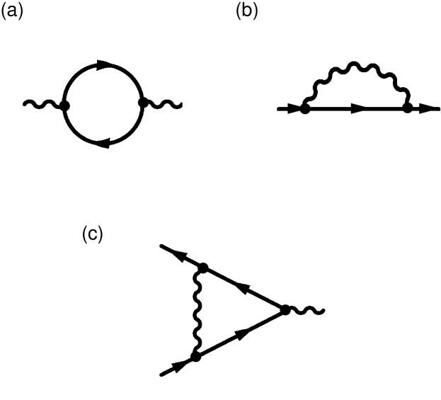
Figure 2: Feynman diagrams at the one loop level. Solid lines represent the fermionic propagator and dashed lines the bosonic propagator. (a) Polarization diagram, describing the bosonic self-energy; (b) fermionic self energy, (c) Vertex corrections.

III.1 One loop calculations

At one loop level, corrections to the different coupling constants in Eq. (12) come from three diagrams: the bosonic polarization bubble, the fermionic self energy and vertex corrections, as shown in Fig. 2. The bosonic polarization depicted in Fig. 2a is given by

$$\Pi_{ij}(q)=g^{2}\,\mathrm{tr}\!\int_{>}dk\,\Gamma_{i}G_{\psi}\left(k\right)\Gamma_{j}G_{\psi}\left(k+q\right),$$ (17)

where $G_{\psi}^{-1}\left(k\right)=-ik_{0}+\mathcal{H}_{0}(k)$ is the bare fermion propagator

$$G_{\psi}\left(k\right)=\frac{-ik_{0}+v_{r}\tilde{k}_{r}\tau_{0}\otimes\sigma_{y}+v_{z}k_{z}\tau_{0}\otimes\sigma_{x}}{k_{0}^{2}+E_{k}^{2}},$$ (18)

$``\text{tr}"$ is the trace and $\int_{>}$ refers to the shell integration defined in Eq. (15). In all cases, $\Pi_{ij}(q)=\delta_{ij}\Pi(q)$ is diagonal and has the same form for any of the Yukawa vertices considered in Eq. (5). To proceed with the integration, it is convenient to parametrize the fermionic momenta as

$$k_{0} =\epsilon\cos\theta$$

$$v_{r}k_{r} =\epsilon\sin\theta\cos\phi$$ (19)

$$v_{z}k_{z} =\epsilon\sin\theta\sin\phi$$

with $\theta\in\left[0,\pi\right]$ and $\phi\in\left[0,2\pi\right]$ and $\epsilon\equiv\sqrt{k_{0}^{2}+E_{k}^{2}}$ defined within the UV shell $\epsilon\in[e^{-zd\ell}\Lambda,\Lambda]$ around the nodal line. As previously stated in the last section, we ignore terms proportional to $q/k_{F}$ in the denominator of the fermionic propagator, namely $(|\mathbf{k}_{r}+\mathbf{q}_{r}|^{2}-k_{F}^{2})/2m\approx v_{r}(\tilde{k}_{r}+q_{r}\cos\theta)$, with $\theta$ the angle between the vectors $\mathbf{k}_{r}$ and $\mathbf{q}_{r}$. Expanding to second order in $q_{0}$, $q_{r}$ and $q_{z}$ and integrating over $k$, we find that

$$\Pi(q)=\Pi_{0}\left(q_{0}^{2}+\frac{1}{2}v_{r}^{2}q_{r}^{2}+v_{z}^{2}q_{z}^{2}\right)zd\ell,$$ (20)

where

$$\Pi_{0}=\frac{4N_{f}g^{2}k_{F}}{3\pi v_{r}v_{z}\Lambda(\ell)}.$$ (21)

Hence, under the RG process the bosonic action (11) is renormalized as

$$d(c_{0}^{2}) =\Pi_{0}zd\ell=d(c_{2}^{2})$$ (22)

$$d(c_{1}^{2}) =\frac{1}{2}\Pi_{0}zd\ell,$$ (23)

whereas the mass term $m_{\phi}$ is not renormalized and can be set to zero at the fixed point, which corresponds to a quantum phase transition.

We also note that the polarization bubble in the CDW, SC and SDW channels has explicit frequency dependence, and is distinct from earlier works that studied the effect of Coulomb interactions in the Yukawa language by decomposing the four fermion interaction in the Hartree channel Huh ; Sur-1 . In the Coulomb case, the bosonic propagator is frequency independent, implying in the absence of renormalization of the fermionic wavefunction. This in turn implies that vertex corrections vanish due to Ward identities that follow from the local gauge invariance of the Yukawa theoryCho . The present Yukawa theory is not locally gauge invariant, and therefore has an intrinsically different RG structure, with distinct fixed points.

The fermionic self energy in Fig. 2b gives corrections to the velocities $v_{r}$ and $v_{z}$:

$$\hat{\Sigma}(k)=-g^{2}\sum_{j=1}^{N_{b}}\int_{>}dq\ \Gamma_{i}G_{\psi}(k-q)\Gamma_{i}G_{\phi}(q),$$ (24)

where

$$G_{\phi}^{-1}\left(q\right)=c_{0}^{2}q_{0}^{2}+c_{1}^{2}(q_{x}^{2}+q_{y}^{2})+c_{2}^{2}q_{z}^{2}$$ (25)

is the bosonic propagator in the disordered phase, and here $\int_{>}$ refers to the shell integration as defined in Eq (16). Expanding to linear order in $k_{0}$, $\tilde{k}_{r}$ and $k_{z}$,

$$\hat{\Sigma}(k)=\tau_{0}\otimes\left(-\Sigma_{0}ik_{0}\sigma_{0}+\Sigma_{r}v_{r}\tilde{k}_{r}\sigma_{y}+\Sigma_{z}v_{z}k_{z}\sigma_{x}\right)zd\ell$$

where

$$\Sigma_{0} =\frac{N_{b}}{N_{f}}\frac{\Lambda}{v_{r}k_{F}}F_{1}\left(g_{0}^{2},g_{1}^{2},g_{2}^{2}\right)=\Sigma_{z}$$ (26)

$$\Sigma_{r} =\frac{N_{b}}{N_{f}}\frac{\Lambda}{v_{r}k_{F}}F_{2}\left(g_{0}^{2},g_{1}^{2},g_{2}^{2}\right).$$ (27)

The functions $F_{1}$, and $F_{2}$ are special functions,

$$F_{1}(a,b,c) = \int_{0}^{\pi}\!d\phi\!\int_{0}^{\pi}\!d\theta\frac{\left(2\pi\right)^{-3}\cos 2\theta\csc\phi}{\frac{1}{b}+\frac{1}{c}\cot^{2}\phi+\frac{1}{a}\cot^{2}\theta\csc^{2}\phi}$$

$$F_{2}(a,b,c) = \int_{0}^{\pi}\!d\phi\!\int_{0}^{\pi}\!d\theta\frac{\left(2\pi\right)^{-3}\left(\cos 2\theta+\cot^{2}\phi\right)\sin\phi}{\frac{1}{b}+\frac{1}{c}\cot^{2}\phi+\frac{1}{a}\cot^{2}\theta\csc^{2}\phi}$$

with

$$g_{n}^{2}\equiv\frac{N_{f}g^{2}k_{F}}{v_{r}v_{z}c_{n}^{2}\Lambda(\ell)},\quad\text{(}n=0,1,2)$$ (28)

defining a set of three dimensionless couplings.

Lastly, the diagram in Fig. 2c describes the corrections to the Yukawa vertex,

$$\Upsilon{}_{j}=g^{3}\sum_{i=1}^{N_{b}}\int_{>}dk\,G_{\phi}(-k)\Gamma_{i}G_{\psi}(k)\Gamma_{j}G_{\psi}(k)\Gamma_{i},$$ (29)

where $\int_{>}$ describes a fermionic momentum shell integration, as defined in Eq. (15). The calculation of this diagram yields

$$\Upsilon_{j}=-\frac{(N_{b}-2)}{N_{f}}g\Gamma_{j}\,F_{3}\left(g_{0}^{2},g_{1}^{2},g_{2}^{2}\right)zd\ell.$$ (30)

where

$$F_{3}(a,b,c)=\int_{0}^{2\pi}\negmedspace\negmedspace d\phi\!\int_{0}^{\pi}\!d\theta\frac{\left(2\pi\right)^{-3}\csc\,\theta}{(\frac{1}{b}\cot^{2}\theta+\frac{1}{c}\sin^{2}\phi+\frac{1}{a}\cos^{2}\phi)}.$$

Due to the symmetry of the integrals around the nodal line that follow from linearly dispersing quasiparticles, no new couplings are generated in the RG flow. With those results, one can proceed to write down the RG equations of the problem.

III.2 RG equations

Absorbing the renormalizations in the bosonic propagator (25) in the form of an anomalous dimension of the bosonic field $\phi$,

$$\eta_{\phi}=\frac{2g_{0}^{2}}{3\pi}z,$$ (31)

the $c_{0}$ coefficient becomes marginal whereas $c_{1}$ and $c_{2}$ renormalize as

$$\frac{d\,\ln c_{1}^{2}}{d\ell}=\frac{2}{3\pi}g_{0}^{2}z\left(\frac{2c_{0}^{2}-c_{1}^{2}}{c_{1}^{2}}\right),$$ (32)

and

$$\frac{d\,\ln c_{2}^{2}}{d\ell}=\frac{4}{3\pi}g_{0}^{2}z\left(\frac{c_{0}^{2}-c_{2}^{2}}{c_{2}^{2}}\right).$$ (33)

Regardless of the flow of the dimensionless coupling $g_{0}^{2}$, it is clear that $\{c_{0}^{2},c_{1}^{2},c_{2}^{2}\}$ flow towards the values $\{c_{0}^{2},2c_{0}^{2},c_{0}^{2}\}$ at the fixed point, where $d\ln c_{1}^{2}/d\ell=d\ln c_{0}^{2}/d\ell=0$, provided that $g_{0}^{2}$ remains finite. From Eq. (28), the ratio between the dimensionless couplings at the fixed point is

$$\frac{g_{1}^{2}}{g_{0}^{2}}=\frac{1}{2},\quad\frac{g_{2}^{2}}{g_{0}^{2}}=1.$$ (34)

Since the nature of the interacting fixed point does not depend on the starting point of the RG flow, we are then allowed to fix the ratio between $g_{0}$, $g_{1}$ and $g_{2}$ at their fixed point values in the RG equations from the start Note ,

$$g_{0}^{2}=2g_{1}^{2}=g_{2}^{2}\equiv\tilde{g}^{2}.$$ (35)

With this restriction in place, we define the special functions

$$F_{m}\left(\tilde{g}^{2},\frac{\tilde{g}^{2}}{2},\tilde{g}^{2}\right):=\alpha_{m}(\tilde{g}^{2}),$$ (36)

with $m=1,$2,3. Those functions are linear in the dimensionless coupling $\tilde{g}^{2}$ defined above.

Similarly, one can absorb the RG corrections to the fermionic propagator by defining the anomalous dimension for the fermionic field $\psi$,

$$\eta_{\psi}=\frac{N_{b}}{N_{f}}\frac{\Lambda}{v_{r}k_{F}}z\,\alpha_{1}(\tilde{g}^{2}),$$ (37)

in such a way that $dv_{z}/d\ell=v_{z}(z-z_{1})=0$ is marginal if we set $z_{1}=z$. The remaining RG equation for the other velocity is

$$\frac{dv_{r}}{d\ell}=v_{r}(z-1)-v_{r}\eta_{\psi}+zv_{r}\Sigma_{r}(\tilde{g}^{2}).$$ (38)

The velocity $v_{r}$ can be kept fixed in the RG flow by renormalizing the dynamical exponent,

$$z=1+\eta_{\psi}-\frac{N_{b}}{N_{f}}\frac{\Lambda}{v_{r}k_{F}}\alpha_{2}(\tilde{g}^{2})+O(1/N_{f}^{2}).$$ (39)

Ignoring terms that are proportional to $\Lambda/v_{r}k_{F}\ll 1$, consintently with prior assumptions about the fermionic propagator in Eq. (20), we have that $\eta_{\psi}=0$ while the dynamical exponent $z=z_{1}=1$ remains similarly unchanged at one loop level. From the preceding analysis, even though $g^{2}$ is marginal, the tree level scaling dimension of $\tilde{g}^{2}$ is

$$[\tilde{g}^{2}]=4z-3=1.$$ (40)

This leads to the one loop RG equation for the dimensionless Yukawa coupling,

$$\frac{d\widetilde{g}^{2}}{d\ell}=\widetilde{g}^{2}\left[1-\frac{2(N_{b}-2)}{N_{f}}\alpha_{3}(\widetilde{g}^{2})-\frac{2}{3\pi}\widetilde{g}^{2}\right],$$ (41)

which determines the nature of the interacting fixed point in the RG flow.

III.3 Fixed point and critical exponents

After a quick inspection, the RG equation (41) flows toward a stable fixed point, where $d\tilde{g}/d\ell=0$. In the $N_{f}\to\infty$ limit, the fixed point is at

$$\tilde{g}_{\infty}^{2}=\frac{3\pi}{2}.$$ (42)

Proceeding in leading $1/N_{f}$ order, the fixed point is

$$\frac{\widetilde{g}_{*}^{2}}{\tilde{g}_{\infty}^{2}}=1-\frac{2(N_{b}-2)}{N_{f}}\alpha_{3}(\tilde{g}_{\infty}^{2}),$$ (43)

where $\alpha_{3}(\tilde{g}_{\infty}^{2})\approx 0.1487$. To compute the correlation length exponent $\nu$, we write down the RG equations for the gapping mass term,

$$\frac{dm_{\phi}^{2}}{d\ell}=(2-\eta_{\phi})m_{\phi}^{2},$$ (44)

which gives as a result

$$\nu=\frac{1}{2-\eta_{\phi}}=1-\frac{2(N_{b}-2)}{N_{f}}\alpha_{3}(\tilde{g}_{\infty}^{2}).$$ (45)

Once two exponents are known, the others can be obtained from hyperscaling relations. The quantum version of the hyperscaling relation for the specific heat exponent gives

$$\alpha=2-\nu\left(2+z\right)=-1+\frac{2(N_{b}-2)}{N_{f}}\alpha_{3}(\tilde{g}_{\infty}^{2}),$$ (46)

where we have set $d=2$ in the general expression $\alpha=2-\nu\left(d+z\right)$, since the fermions are scaled in only 2 spatial directions around the nodal line. Moreover, $d=2$ gives the correct large $N_{f}$ behavior, as we show below from the mean field analysis.

								Exponent								value
								$z$								1
								$\eta_{\phi}$								$1-0.2975\frac{(N_{b}-2)}{N_{f}}$
								$\eta_{\psi}$								0
								$\alpha$								$-1+0.2975\frac{(N_{b}-2)}{N_{f}}$
								$\beta$								$1-0.1487\frac{(N_{b}-2)}{N_{f}}$
								$\gamma$								$1$
								$\delta$								$2+0.1487\frac{(N_{b}-2)}{N_{f}}$
								$\nu$								$1-0.2975\frac{(N_{b}-2)}{N_{f}}$

Table 1: List of critical exponents for nodal-line semimetals including $1/N_{f}$ corrections, with $N_{f}$ the number of fermionic flavors and $N_{b}$ the number of components of the bosonic fields. $N_{b}=1$: Charge density wave order; $N_{b}=2$: superconductivity; $N_{b}=3$: spin density wave.

Fisher’s and Widom’s equality are the same as in the classical case. Fisher’s equality gives the exponent

$$\gamma=(2-\eta_{\phi})\nu=1+O(1/N_{f}^{2}).$$ (47)

Essam-Fisher relation $\alpha+2\beta+\gamma=2$ gives the order parameter exponent in one loop

$$\beta=1-\frac{(N_{b}-2)}{N_{f}}\alpha_{3}(\tilde{g}_{\infty}^{2}).$$ (48)

Finally, Widom’s equality gives the field exponent

$$\delta=1+\frac{\gamma}{\beta}=2+\frac{(N_{b}-2)}{N_{f}}\alpha_{3}(\tilde{g}_{\infty}^{2}).$$ (49)

The set of exponents for the three different gapped instabilities and their numerical values is listed in Table I. In nodal line semimetals, where the existence of a Fermi surface leads the anomalous dimension of the fermions $\eta_{\psi}$ to vanish in one loop, the only source of renormalization comes from the vertex correction, which is zero when $N_{b}=2$. It is clear that in the SC case, where the order parameter is complex ($N_{b}=2$), all one loop corrections vanish, implying that the mean field results are exact up to $O(N_{f}^{-2})$ terms. In both the CDW ($N_{b}=1$) and SDW ($N_{b}=3$) order, the one loop corrections are finite and have opposite signs.

As a consistency check, one can explicitly verify that the mean field exponents are correctly recovered in the $N_{f}\to\infty$ limit. Taking the bosonic fields at their mean-field value $\phi_{0}$ and integrating out the fermions, the mean field free energy for a generic gapped phase at the nodal line is

$$\mathcal{F}_{\text{MF}}(\phi_{0})=\frac{\phi_{0}^{2}}{g}-\int_{\tilde{k}_{r}^{2}+k_{z}^{2}<\Lambda}d\vec{k}\sqrt{\tilde{k}_{r}^{2}+k_{z}^{2}+\phi_{0}^{2}},$$ (50)

where $\vec{k}$ are the spatial components of the momentum away from the nodal line, after conveniently absorbing the velocities $v_{r}$ and $v_{z}$ in their definition. We proceed by expanding (50) in powers of the order parameter $\phi_{0}$ and also in terms of long-wavelength spatial modulations that couple to momenta as gauge fields. The corresponding Ginzburg-Landau free energy for nodal-line semimetals has the usual form expected for conventional Dirac fermions in 2D Sachdev ,

$$\mathcal{F}_{\text{GL}}(\phi_{0})=\tilde{q}_{r}^{2}|\phi_{0}|+q_{z}^{2}|\phi_{0}|+a_{0}\left(\frac{g_{c}-g}{g}\right)\left|\phi_{0}\right|^{2}+b\left|\phi_{0}\right|^{3},$$ (51)

where $a_{0}$ and $b$ are positive numbers, and $g_{c}$ is the critical coupling of the mean field theory. Minimization of the free energy in the order parameter $|\phi_{0}|$ implies that $\left|\phi_{0}\right|\sim\left|g_{c}-g\right|$ giving $\beta=1$ at the mean field level. At the same time, by dimensional analysis

$$\xi^{-2}|\phi_{0}|\cong\delta g|\phi_{0}|^{2},$$ (52)

and hence the correlation length $\xi\sim(\delta g)^{-1}$ diverges with the mean field exponent $\nu=1$. Using hyperscaling relations, all other mean field exponents can be recovered and found to be in agreement with the large $N_{f}$ results in the $N_{f}$$\rightarrow\infty$ limit, indicating that hyperscaling relations are fulfilled.

IV CONCLUSIONS

In summary, we performed a Wilson momentum shell RG calculation and computed the scaling exponents describing the universal quantum critical behavior for 3D nodal-line semimetals with linear band crossings. We considered states that lead to fully gapped instabilities in the charge, spin and $s$-wave superconducting channels, and calculated their exponents in a unified manner.

A few comments about the RG literature in nodal-line semimetals is in order. Previous perturbative RG calculations in Ref. Huh ; Wang-1 examined the problem of Coulomb interactions within the Yukawa method for a nodal-line. In those works, a non-interacting fixed point was found in the clean case, with logarithmic corrections to scaling, indicating that Coulomb interactions are marginally irrelevant, as in graphene Kotov .

In the strong coupling regime, Ref. Sur-1 addressed the problem of broken symmetry states for a nodal-line both in the superconducting and in the particle-hole channels. That work considered the effect of short range interactions through an $\epsilon$-expansion in the fermionic language. In that approach, short range interactions are irrelevant operators in the perturbative regime, but flow towards an interacting fixed point when they are sufficiently strong. The fermionic language is particularly suitable to address the competition between different channels of instability, but not so convenient to address the universal quantum critical scaling of the phases. Here, we used a non-perturbative Gross-Neveau-Yukawa theory involving order parameter bosonic fields to examine the quantum critical scaling of various gapped phases in nodal-line semimetals. After deriving the interacting fixed points of this theory, we extracted the full set of quantum critical exponents. Those exponents reduce to their mean-field values in the $N_{f}\to\infty$ limit, suggesting that hyperscaling is satisfied.

The RG calculations were performed in one loop in the number of fermionic flavors $N_{f}$, which were added for analytic control. We found that in the SC state, where vertex corrections are absent, the mean-field exponents are exact within one loop, whereas the CDW and SDW states have finite $1/N_{f}$ corrections with opposite signs. In all cases, the dynamical exponent $z=1$ in leading order, whereas the one loop corrections to various exponents follow directly from the bosonic anomalous dimension $\eta_{\phi}$. This study complements current efforts in the literature to account for the effect of electronic correlations in nodal systems and addresses a timely class of materials with topological nodal lines.

V ACKNOWLEDGEMENTS

The authors thank R. Nandkishore and F. Kruger for illuminating conversations. BU acknowledges Carl T. Bush fellowship at University of Oklahoma for partial support.

References

- (1) A. H. Castro Neto, N. M. R. Peres, K. S. Novoselov, and A. K. Geim, Rev. Mod. Phys. 81,109 (2009).
- (2) X. Wan, A. M Turner, A. Vishwanath, and S. Y Savrasov, Phys. Rev. B 83, 205101 (2011).
- (3) N. P. Armitage, E. J. Mele, and A. Vishwanath, Rev. Mod. Phys. 90, 1443 (2018).
- (4) C. Fang, H. Weng, X. Dai and Z. Fang, 2016 Chinese Phys. B 25 11710 (2016).
- (5) S.-Y. Yang, H. Yang, E. Derunova, S. S. P. Parkin, B. Yan, M. N. Ali, Advances in Physics: X, 3:1, (2018)
- (6) Y.-H. Chan, Ching-Kai Chiu, M. Y. Chou, and A. P. Schnyder, Phys. Rev. B 93, 205132.
- (7) Z. Wang, Y. Sun, X Q Chen, C. Franchini, G. Xu, H. Weng, X. Dai and Z. Fang, Phys. Rev. B 85 195320 (2012).
- (8) Ching-Kai Chiu, Jeffrey C. Y. Teo, Andreas P. Schnyder, and Shinsei Ryu, Rev. Mod. Phys. 88, 035005 (2016).
- (9) D. P. Arovas and F. Guinea, Phys. Rev. B 78, 245416 (2008).
- (10) T. T. Heikkila and G. E. Volovik, JETP Lett. 93, 59 (2011).
- (11) A. A. Burkov, M. D. Hook, and L. Balents, Phys. Rev. B 84, 235126 (2011).
- (12) G. Xu, H.M. Weng, Z. J. Wang, X. Dai and Z. Fang, Phys. Rev. Lett. 107 186806 (2011).
- (13) K. Mullen, B. Uchoa, D. Glatzhofer, Phys. Rev. Lett. 115, 026403 (2015).
- (14) H. Weng, Y. Liang, Q. Xu, R. Yu, Z. Fang, X. Dai, Y. Kawazoe, Phys. Rev. B 92, 045108 (2015).
- (15) Y. Kim, B. J. Wieder, C. L. Kane, and Q. D. A. M. Gibson, A. Rappe, Phys. Rev. Lett. 115, 036806 (2015).
- (16) H. Weng, C. Fang, Z. Fang, B. A. Bernevig, and X. Dai Phys. Rev. X 5, 011029 (2015).
- (17) L. S. Xie, L. M. Schoop, E. M. Seibel, Q. D. Gibson, W. Xie, R. J. Cava, APL Mat. 3, 083602 (2015).
- (18) G. Bian, T.-R. Chang, R. Sankar, S.-Y. Xu, H. Zheng, T. Neupert, C.-K. Chiu, S.-M. Huang, G. Chang, I. Belopolski, D. S. Sanchez, M. Neupane, N. Alidoust, C. Liu, B. Wang, C.-C. Lee, H.-T. Jeng, C. Zhang, Z. Yuan, S. Jia, A. Bansil, F. Chou, H. Lin and M. Z. Hasan, Nat. Comm. 7, 10556 (2016).
- (19) G. Bian, T.-R. Chang, H. Zheng, S. Velury, S.-Y. Xu, T. Neupert, C.-K. Chiu, S.-M. Huang, D. S. Sanchez, I. Belopolski, N. Alidoust, P.-J. Chen, G. Chang, A. Bansil, H.-T. Jeng, H. Lin, and M. Z. Hasan, Phys. Rev. B 93, 121113(R) (2016).
- (20) Q. Yan, R. Liu, Z. Yan, B. Liu, H. Chen, Z. Wang, and Ling Lu, Nat. Phys. 14, 461 (2018).
- (21) B.-B. Fu, C.-J. Yi, T.-T. Zhang, M. Caputo, J.-Z. Ma, X. Gao, B. Q. Lv, L.-Y. Kong, Y.-B. Huang, P. Richard, M. Shi, V. N. Strocov, C. Fang, H.-M. Weng, Y.-G. Shi, T. Qian, and H. Ding, Science Advances 5, 1126 (2019).
- (22) W. Deng, J. Lu, F. Li, X. Huang, M. Yan, J. Ma & Z. Liu, Nat. Comm. 10, 1769 (2019).
- (23) L. Lu, L. Fu, J. D. Joannopoulos, and M. Soljačić, Nat. Photonics 7, 294 (2013).
- (24) B. Song, C. He, S. Niu, L. Zhang, Z. Ren, X.-J. Liu, and G.-B. Jo, Nat. Phys. 15, 911 (2019).
- (25) V. N. Kotov, B. Uchoa, V. M. Pereira, F. Guinea, and A. H. Castro Neto, Rev. Mod. Phys. 84, 1067 (2012).
- (26) A. Sekine, T. Z. Nakano, Y. Araki, and K. Nomura, Phys. Rev. B 87, 165142 (2013).
- (27) P. Goswami and S. Chakravarty, Phys. Rev. Lett. 107, 196803 (2011).
- (28) P. Hosur, S. A. Parameswaran, and A. Vishwanath, Phys. Rev. Lett. 108, 046602 (2012).
- (29) R. E. Throckmorton, J. Hofmann, E. Barnes, and S. Das Sarma, Phys. Rev. B 92, 115101 (2015).
- (30) J. Gonzalez, Phys. Rev. B 90, 121107(R) (2014).
- (31) H. Isobe, B.-J. Yang, A. Chubukov, J. Schmalian, and N. Nagaosa, Phys. Rev. Lett. 116, 076803 (2016).
- (32) E. G. Moon, C. Xu, Y. B. Kim, and L. Balents, Phys. Rev. Lett. 111, 206401 (2013).
- (33) Igor F. Herbut and Lukas Janssen Phys. Rev. Lett. 113, 106401 (2015).
- (34) Y. Huh, E.-G. Moon and Y. B. Kim, Phys. Rev. B 93, 035138 (2016).
- (35) Y. Wang and R. Nandkishore, Phys. Rev. B 96, 115130 (2017).
- (36) B. Yang, E. Moon, H. Isobe and N. Nagaosa, Nat. Phys 10, 774 (2014).
- (37) I. F. Herbut, Phys. Rev. Lett. 97, 146401 (2006).
- (38) F. F. Assaad and I. F. Herbut, Phys. Rev. X 3, 031010 (2013).
- (39) G. Montambaux, F. Piéchon, J.-N. Fuchs, and M. O. Goerbig, Phys. Rev. B 80, 153412 (2009).
- (40) M. D. Uryszek, E. Christou, A. Jaefari, F. Krüger and B. Uchoa, Phys. Rev. B, 100, 155101 (2019).
- (41) B. Roy and M. S. Foster Phys. Rev. X 8, 011049 (2018).
- (42) S. Sur and B. Roy Phys. Rev. Lett. 123, 207601 (2019).
- (43) B. Uchoa, and K. Seo, Phys. Rev. B 96, 220503(R) (2017).
- (44) B. Roy, P. Goswami, and V. Juričić, Phys. Rev. B 95, 201102(R) (2018).
- (45) R. Nandkishore Phys. Rev. B 93, 020506(R) (2016).
- (46) B. Roy Phys. Rev. B 96, 041113(R) (2017).
- (47) S. Raghu, X.-L. Qi, C. Honerkamp, and S.-C. Zhang, Phys. Rev. Lett. 100, 156401 (2008).
- (48) E. Christou, B. Uchoa, F. Kruger, Phys. Rev. B 98, 161120(R) (2018).
- (49) S. W. Kim, K. Seo, B. Uchoa, Phys. Rev. B 97, 201101(R) (2018).
- (50) R. Okugawa and S. Murakami, Phys. Rev. B 96, 115201 (2017).
- (51) S. Sur and R. Nandkishore, New J. Phys. 18, 115006 (2016).
- (52) G. Young Cho, and E.-G. Moon, Scientific Reports 6, 19198 (2016).
- (53) One could equivalently solve the RG equations for three independent couplings. That procedure leads to the same conclusions regarding the fixed point.
- (54) S. Sachdev, Quantum Phase Transitions, 2nd ed. (Cambridge University Press, Cambridge, UK, 2011).