Topological States in Generalized Electric Quadrupole Insulators

Abstract

The modern theory of electric polarization has recently been extended to higher multipole moments, such as quadrupole and octupole moments. The higher electric multipole insulators are essentially topological crystalline phases protected by underlying crystalline symmetries. Henceforth, it is natural to ask what are the consequences of symmetry breaking in these higher multipole insulators. In this work, we investigate topological phases and the consequences of symmetry breaking in generalized electric quadrupole insulators. Explicitly, we generalize the Benalcazar-Bernevig-Hughes model by adding specific terms in order to break the crystalline and non-spatial symmetries. Our results show that chiral symmetry breaking induces an indirect gap phase which hides corner modes in bulk bands, ruining the topological quadrupole phase. We also demonstrate that quadrupole moments can remain quantized even when mirror symmetries are absent in a generalized model. Furthermore, it is shown that topological quadrupole phase is robust against a unique type of disorder presented in the system.

I Introduction

Electric polarization in crystalline had traditionally been a long-standing issue as it is not a well-defined observable that can simply be given by the expectation value of a local operator Resta94rmp ; Resta98prl . The modern theory of bulk polarization is based on the Berry phase, which is determined via the wave functions of energy bands over a closed path in the Brillouin zone King93prb . The theory has exerted a strong influence on condensed matter physics over recent decades, particularly on the development of topological band insulators XiaoD10rmp ; Kane10rmp ; QiXL11rmp ; SQS ; BernevigBook ; Thouless83prb ; FuL06prb . Recent studies have extended the modern theory of polarization to higher multipole moments, such as quadrupole and octupole moments. As is well known, quantized bulk polarization in the Su-Schrieffer-Heeger (SSH) model gives rise to the fractional charge $\pm e/2$ at the boundaries of a one-dimensional (1D) sample, where $e$ is the electron charge SSH79prl . Benalcazar et al. extended this to two- and three-dimensional systems that hold quantized bulk quadrupole and octupole moments, respectively Benalcazar17Science ; BBH17prb . These systems are denoted as electric quadrupole and octupole insulators. Explicit models demonstrate that these quantized bulk multipole moments also manifest fractionalized boundary charges. Traditionally, a topological bulk state in a $d$-dimensional system has robust ($d-1$) dimensional boundary states. Nevertheless, topological quadrupole (octupole) insulators have localized states at corners, namely, the $d-2$ ($d-3$) boundaries of the system. This “high-order” bulk-boundary correspondence Trifunovic19prx casts these topological phases into a new class of topological insulators denoted as “high-order topological insulators” Schindler18SA . Generally, a $d$-dimensional high-order topological insulator has non-trivial boundary states at the $d-m$ boundary ($d\geq m\geq 2$). Thus, such high-order topological insulators have attracted much theoretical and experimental interest over the past few years Langbehn17prl ; Khalaf18prb ; SongZD19prl ; Geier18prb ; petrides2019arxiv ; WangZJ19prl ; Schindler18NP ; Serra-Garcia18nature ; Peterson18nature ; Franca18prb ; Thomale18np , and have been extended to high-order topological superconductors YanZB18prl ; WangQ18prl ; Hsu18prl ; Volpez19prl ; LiuT18prb ; ZhuXY18prb ; Shapourian18prb and even semi-metals Ezawa18prl ; okugawa2019arxiv ; wieder2019arxiv .

Higher electric multipole insulators are essentially topological crystalline insulators FuL11prl ; Neupert18springer ; Jan17prx , with the quantization of multipole moments imposed via the underlying crystalline symmetries of the system. For example, the quantization of quadrupole (octupole) moments of the Benalcazar-Bernevig-Hughes (BBH) model can be performed using a combination of mirror symmetries BBH17prb . As well as crystalline symmetries, high-order topological insulators may also require non-spatial symmetries (i.e., chiral, time-reversal, and particle-hole symmetries) in order to protect their high-order topology Schindler18SA ; Yoshida18prb ; Khalaf18prx . A key topic of interest is the determination of the consequences of symmetry breaking, including both the crystalline and non-spatial symmetries, in higher electric multipole insulators. In simple terms, crystalline symmetry breaking damages topological phases while non-spatial symmetry breaking is irrelevant. However, the consequences are in fact more complicated. Furthermore, the high-order topology in the BBH model is characterized by the so-called “nested Wilson loop”. This characterization is based on the equivalent topology between the Wannier bands and the edge spectrum YuR11prb ; Fidkowski11prl ; Alexandradinata14prb ; khalaf19arxiv . The equivalence, however, may be lost under certain circumstances Yang19arxiv ; Yang2019arxiv . In this case it is also meaningful to ask how to demonstrate high-order phase if nested Wilson loop approach fails.

In this paper, we exploit several generalized BBH models in order to evaluate newly appearing topological phases as well as the consequences of symmetry breaking in electric quadrupole insulators. In the first generalized model, we include additional hopping terms to break chiral symmetry. These chiral symmetry breaking terms lead the system to an indirect gap phase. Corner modes will be buried by bulk bands in the indirect gap phase, and quadrupole moments are not well defined. The nested Wilson loop approach fails to capture this phase since there is no real topological phase transition. In the second model, we include hopping terms with imaginary amplitudes in order to break the time-reversal and chiral symmetries. Following an induced phase transition, the equivalent topology between the Wannier bands and edge spectrum may be lost in this simple model. In this case, the nested Wilson loop approach is no longer applicable since its basis is ruined, while the quantized quadrupole moments together with edge polarization and fractional corner charges remain effective for the characterization of high-order topology. In the third model, we focus on mirror symmetry breaking while keeping inversion symmetry. Unexpectedly, the quadrupole moments remain quantized, despite the breakdown of mirror symmetry. Note that the $C_{2}$ (inversion) symmetry is kept for all these three models, and it is necessary for the well-defined quadrupole moments. More interestingly, we determine the quantized quadrupole moments to be robust against disorders of a unique type added to the system.

The remainder of this paper is organized as follows. Sec. II introduces the extended model with chiral symmetry breaking, and discusses the consequences of the indirect gap phase. Sec. III presents the inclusion of time-reversal and chiral symmetry breaking in the model. Sec. IV details the results of mirror symmetry breaking. Sec. V considers the robustness of quantized quadrupole moments in the presence of disorders. Finally, Sec. VI concludes our results with a discussion.

II Indirect gap phases: chiral symmetry breaking

The topology of the SSH model, which forms the basis of the BBH model, is protected by chiral symmetry. Thus, in this section we consider a generalized BBH model with chiral symmetry breaking by introducing hopping terms between equivalent sites, as presented in Fig. 1(a). The dressed model is expressed as follows:

$$H_{1}=H_{0}+\sum_{\mathbf{R}}\text{$\sum_{\zeta=1}^{4}\sum_{s=x,y}$}t(C_{\mathbf{R},\zeta}^{\dagger}C_{\mathbf{R}+\hat{s},\zeta}+\mathrm{H.c.}),$$ (1)

where $t$ is the corresponding hopping amplitude, and

$$H_{0}= \sum_{\mathbf{R}}\Big{[}\gamma_{x}(C_{\mathbf{R},1}^{\dagger}C_{\mathbf{R},3}+C_{\mathbf{R},2}^{\dagger}C_{\mathbf{R},4})$$

$$+\gamma_{y}(C_{\mathbf{R},1}^{\dagger}C_{\mathbf{R},4}-C_{\mathbf{R},2}^{\dagger}C_{\mathbf{R},3})$$

$$+\lambda(C_{\mathbf{R},1}^{\dagger}C_{\mathbf{R}+\hat{x},3}+C_{\mathbf{R},4}^{\dagger}C_{\mathbf{R}+\hat{x},2})$$

$$+\lambda(C_{\mathbf{R},1}^{\dagger}C_{\mathbf{R}+\hat{y},4}-C_{\mathbf{R},3}^{\dagger}C_{\mathbf{R}+\hat{y},2})\Big{]}+\mathrm{H.c.},$$ (2)

The operators $C_{\mathbf{R},\zeta}^{\dagger}$ ($C_{\mathbf{R},\zeta}$) are creation (annihilation) operators at unit cell $\mathbf{R}=(m\hat{x},n\hat{y})$ with $\zeta=1,2,3,4$ being orbital-like degree of freedoms. Here the parameters $\gamma_{x,y}$ and $\lambda$ are hopping amplitudes within and between unit cells, as sketched in Fig. 1(a). The Hamiltonian $H_{0}$ represents the original BBH model. Note the lattice constant is assumed to be unity and $\lambda=1$ throughout the following sections.

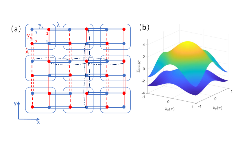
Figure 1: (a) Lattice structure of extended BBH model $H_{1}$. The dashed dark blue lines represent hopping at equivalent sites with strength $t$ between nearest unit cells. For simplicity, here we only sketch parts of this kind of hopping. (b) Energy bands corresponding to (a) with parameters fixed at $\gamma_{x}=\gamma_{y}=0.5,$ and $t=0.5$. Here the system has an indirect gap.

The corresponding Bloch Hamiltonian in momentum space is described as follows:

$$H_{1}({\bf k})=H_{q}({\bf k})+2t\sum_{s=x,y}\cos k_{s},$$ (3)

where

$$H_{q}({\bf k}) =[\gamma_{x}+\lambda\cos k_{x}]\Gamma_{4}+\lambda\sin k_{x}\Gamma_{3}$$

$$+[\gamma_{y}+\lambda\cos k_{y}]\Gamma_{2}+\lambda\sin k_{y}\Gamma_{1}.$$ (4)

The Gamma matrices are defined as $\Gamma_{j}=-\tau_{2}\sigma_{j}$ ($j=1,2,3$), and $\Gamma_{4}=\tau_{1}\sigma_{0}$ with $\tau$ and $\sigma$ both being Pauli matrices for the unit cell orbital degrees of freedom. Due to the appearance of identity terms in Eq. (3), chiral symmetry is no longer preserved. One can check that

$$\mathcal{C}H_{1}({\bf k})\mathcal{C}^{-1}\neq-H_{1}({\bf k}),\ \mathcal{C}=\tau_{3}\sigma_{0},$$ (5)

where $\mathcal{C}$ is the chiral symmetry operator. Particle-hole symmetry is not preserved either, which is obvious from the energy spectrum $E_{\pm}=2t\sum_{s=x,y}\cos k_{s}\pm\sqrt{\epsilon_{x}^{2}(k_{x})+\epsilon_{y}^{2}(k_{y})}$ where $\epsilon_{s}^{2}(k_{s})=\gamma_{s}^{2}+2\gamma_{s}\lambda\cos k_{s}+\lambda^{2}$. Since the system respects both time-reversal symmetry and inversion symmetry, its energy bands are still doubly degenerated. The global symmetries cast the system into AI class, and its classification is trivial in two-dimensional (2D) Schnyder08prb ; ChiuCK16rmp . Note that Eq. (3) keeps mirror symmetries.

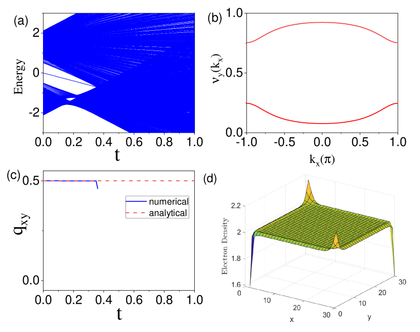
Figure 2: Indirect gap phase induced by chiral symmetry breaking. (a) Energy spectrum of $H_{1}$ as functions of parameter $t$. (b) Wannier bands for fixed $t=0.5$. (c) Calculated quadrupole moments when varying parameter $t$ (red line is calculated analytically with nested Wilson loop approach, blue line is calculated numerically under periodic boundary condition with size $L_{x}\times L_{y}=40\times 40$). (d) Electron charge density in the nontrivial phase with $t=0.2$. Other parameters are $\gamma_{x}=\gamma_{y}=0.5$.

Due to the breakdown of chiral symmetry, the emerging “new phase” is an indirect gap phase chen17arxiv ; LiLH14prb ; Prezgonzlez18arxiv . Figure 1(b) demonstrates that the valence band $E_{\mathrm{max}}^{\mathrm{v}}$ maximum exceeds the conduction band $E_{\mathrm{min}}^{\mathrm{c}}$ minimum. However, there is no bulk gap closure. We denote this phase as an indirect gap phase. The appearance of the indirect gap phase is determined by the following inequality:

$$t>\frac{1}{8}\sum_{\alpha=\pm}\sqrt{\sum_{s=x,y}(\gamma_{s}+\alpha\lambda)^{2}}.$$ (6)

The topological phase of an electric quadrupole insulator is characterized by quadrupole moments $q_{xy}$ Benalcazar17Science ; BBH17prb . Classically, the quadrupole moments are defined as $q_{ij}=\int d^{3}r\rho(r)r_{i}r_{j}$ where $\rho(r)$ is the charge density and $r_{i,j}$ are positions with $i,j=x,y$. Benalcazar et al. proposed insulators having only nonvanishing $q_{xy}$ which is quantized by mirror symmetries. Quadrupole moments will manifest hierarchical observable properties such as edge polarizations (see Appendix B.3) and corner charges (see Appendix B.4). Note that the indirect gap phase here can hide the corner modes in real space. Despite the varying of parameter $t$, the appearance of indirect gap phase is not reflected by the Wannier sector polarization ${\bf p}^{\nu}$ (see Appendix B.2) or the quadrupole moments $q_{xy}$ calculated using nested Wilson loop (see Appendix B.5). In addition, Fig. 2(b) shows that the Wannier bands are not affected by the increase of parameter $t$ at all. This is a reasonable observation since no real gap closure process occurs, and the eigen states are unchanged as the second term proportional to $t$ in Eq. (3) is an identity term. Thus, Eq. (23) in Appendix B.1 indicates that the Wannier bands will be independent of parameter $t$.

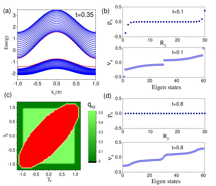
Figure 3: Signatures of the indirect gap phase of Hamiltonian $H_{1}$. (a) Energy spectrum of $H_{1}$ at a ribbon with width $L_{y}=20$ for $t=0.35$. Red lines denote edge states. Panels (b) and (d) plot the edge polarization and Wannier centers of states for $t=0.1$ and $0.8$, respectively. (c) Phase diagram modified by the chiral breaking term in $H_{1}$ with fixed parameter $t=0.38$. Here $q_{xy}$ is calculated numerically under periodic boundary condition with size $L_{x}\times L_{y}=30\times 30$. Red color region denotes indirect gap phases. Other parameters are $\gamma_{x}=\gamma_{y}=0.5$.

Alternatively, we also employ a real-space recipe to calculate the electric quadrupole moment Kang19prb ; Wheeler19prb , which is numerically calculated as follows:

$$q_{xy}=\frac{1}{2\pi}\mathrm{Imlog}\langle\Psi_{G}|\hat{U}_{2}|\Psi_{G}\rangle,$$ (7)

where $|\Psi_{G}\rangle$ is the many-body ground states, and $\hat{U}_{2}\equiv\exp[i2\pi\hat{q}_{xy}]$ with $\hat{q}_{xy}=\sum_{{\bf R}}xy\hat{n}({\bf R})/(L_{x}L_{y})$ as quadrupole momentum density operator per unit cell at position ${\bf R}$. Here $L_{s=x,y}$ are the length of sample along $\hat{s}$ direction. Note that we need to eliminate the atomic limit contribution roy19arxiv . Despite its defects Ono19prb , this technique proves to be effective.

We now further evaluate Fig. 2. Prior to entering the indirect gap phase, the quantized quadrupole moments $q_{xy}=1/2$ remain, accompanied by sharply localized corner states (see Appendix B.4). At the same time, the corresponding energy of the corner states is shifted away from zero-energy. Figure 2(d) shows that the charge density is not “symmetric” with respect to different corners, yet the integrated charge over a quarter of the sample around each corner still quantizes to $\pm e/2$. After the “transition” point, the corner states are hidden by bulk valence bands, and the quantized quadrupole moments are destroyed. The buried corner states work similarly as hidden helical edge states in topological insulators LiC18prb ; Skolasinski18prb . In this case, there are no gaps in the system, thus the real-space recipe is not applicable.

It is evident that the original non-trivial phases (see Appendix B.6) will shrink due to the appearance of indirect gap phases. As demonstrated in the energy spectrum in Fig. 3(a), the conduction bands “overlap” with the valence bands, and the edge states merge to bulk bands. The phase diagram Fig. 3(c) presents a closed region that represents the indirect gap phase, which is consistent with the restriction condition of Eq. (6). Furthermore, both the edge polarization $p_{x}(R_{y})$ (see Appendix B.3) and the Wannier values of states $\nu_{x}$ (see Appendix B.1) can aid in the detection of topological phases. Note that $p_{x}$ and $\nu_{x}$ are calculated on a ribbon with a finite width. Prior to entering the indirect gap phase, $p_{x}(R_{y})$ exhibits non-zero values, with an integrated value over half of the ribbon width as $\pm e/2$. Moreover, there are two isolated topological modes associated with the Wannier center $\nu_{x}=\pm 1/2$. In contrast, for the indirect gap phase with larger $t$, the edge polarization vanishes, and the quantized Wannier value states disappear. This is because the edge states totally merge into the bulk bands.

III Discrepant topology between Wannier bands and edge spectrum

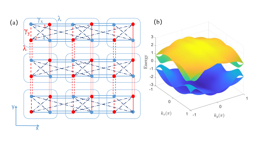
Figure 4: (a) Lattice structure of extended BBH model $H_{2}$. The dashed dark blue lines represent hopping within and between unit cells. These hopping with imaginary amplitudes will break time-reversal symmetry. (b) Energy bands corresponding to (a) with parameters fixed at $\gamma_{x}=0.8,\gamma_{y}=0.5,$ and $J_{2}=0.3.$ The band degeneracy is lifted.

In this section, we consider the consequences of non-spatial symmetry breaking (time-reversal and chiral symmetry) in the second generalized BBH model. The imaginary hopping terms are introduced as depicted in Fig. 4(a). The corresponding modified Hamiltonian is described as follows:

$$H_{2} =H_{0}+\sum_{\mathbf{R}}J_{2}(iC_{\mathbf{R},2}^{\dagger}C_{\mathbf{R},1}-iC_{\mathbf{R},4}^{\dagger}C_{\mathbf{R},3}+\mathrm{H.c.})$$

$$+\sum_{\mathbf{R}}J_{2}(-iC_{\mathbf{R},2}^{\dagger}C_{\mathbf{R}+\hat{x},1}-iC_{\mathbf{R},3}^{\dagger}C_{\mathbf{R}+\hat{x},4}+\mathrm{H.c.}),$$ (8)

where $iJ_{2}$ is the imaginary hopping amplitude ($J_{2}$ is a real number). It is imaginary due to the enclosed half-$\pi$ flux, with the sign convention as in Eq. (8). In the original BBH model, there is $\pi$ flux threading each square plaquette to open band gap, thus for our extended model, we can choose a gauge such that the triangle, for example, triangle with points $1\rightarrow 2\rightarrow 4\rightarrow 1$ in Fig. 4, contains half-$\pi$ flux. The hopping terms with imaginary amplitudes break the time-reversal symmetry Haldane88prl . For simplicity, only $iJ_{2}$ hopping along the $x$ direction is considered, and we assume the same amplitudes within and between unit cells.

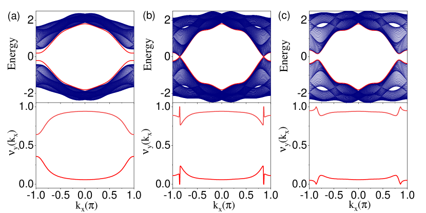
Figure 5: Edge spectrum and corresponding Wannier bands for extended model $H_{2}$. (a) $J_{2}=0.2$. (b) $J_{2}=0.5$. Gap closure happens both at edge spectrum and Wannier bands. (c) $J_{2}=0.6$. Edge spectrum opens a gap while Wannier bands are still gapless. Other parameters are fixed at $\gamma_{x}=0.8,\gamma_{y}=0.5$ for all.

The Fourier transformation of $H_{2}$ from real space to momentum space provides us with the corresponding Bloch Hamiltonian:

$$H_{2}({\bf k})=H_{q}({\bf k})+J_{2}(1-\cos k_{x})\text{$\Gamma_{24}$}+J_{2}\sin k_{x}\Gamma_{23},$$ (9)

where the Gamma matrices are defined as $\Gamma_{ab}=-i\Gamma_{a}\Gamma_{b}$. Here $\Gamma_{24}$ ($\Gamma_{23}$) is odd (even) under time-reversal symmetry, and thus we have:

$$\mathcal{T}H_{2}({\bf k})\mathcal{T}^{-1}\neq H_{2}(-{\bf k}),\ \mathcal{T}=K,$$ (10)

where $\mathcal{T}$ is the time-reversal operator and $K$ represents complex conjugation. Chiral symmetry $\mathcal{C}$ is also not preserved, while particle-hole symmetry is respected with its operator $\mathcal{P}=\tau_{3}\sigma_{0}K$ given as the production of $\mathcal{C}$ and $\mathcal{T}$. Here the bulk bands lose their double degeneracy (Fig. 4(b)). Crucially, the additional terms in Eq. (9) maintain mirror symmetry $\mathcal{M}_{x,y}$.

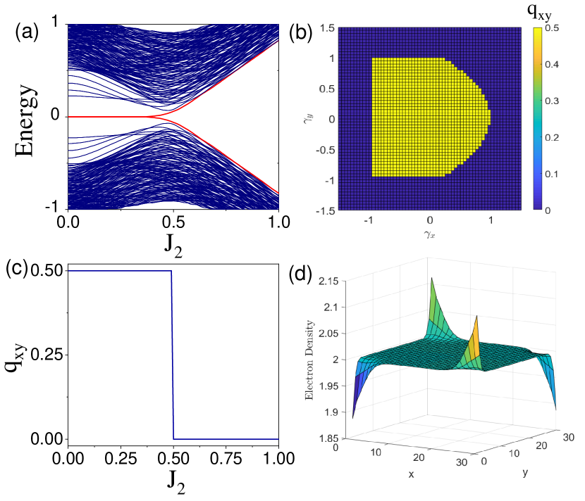
Figure 6: The topological phase transition induced by $iJ_{2}$ hopping terms. (a) Energy spectrum as function of $J_{2}$. We find that the zero-energy mode splits around $J_{2}=0.5$ due to topological phase transition. (b) Calculated quadrupole moments $q_{xy}$ for fixed parameter $J_{2}=0.5$. The nontrivial regions shrink due to topological phase transitions. (c) Numerically calculated $q_{xy}$ corresponding to (a). Here $q_{xy}$ jumps from one-half to zero around $J_{2}=0.5$. (d) Electron charge density in the nontrivial phase for $J_{2}=0.2$. Other parameters are fixed at $\gamma_{x}=0.8,\gamma_{y}=0.5$ for all. Here we set system at size $L_{x}\times L_{y}=40\times 40$ with periodic boundary for the calculation of $q_{xy}$.

Two key points should be noted regarding the extended model $H_{2}({\bf k})$. First, topological equivalence between the edge spectrum and the Wannier bands may be lost in this model. It has been suggested that the Wannier bands (e.g. $\nu_{y}(k_{x})$) can be continuously mapped to the edge spectrum localized at, for example, the $y$-normal boundaries Neupert18springer . In other words, the edge spectrum at the $y$-normal boundaries should be topologically equivalent to Wannier bands $\nu_{y}(k_{x})$. However, in our case, this is not necessarily true. In Fig. 5(a), the edge spectrum (red lines in the top panel of Fig. 5) along the $x$ direction closes its gap as we tune $J_{2}$ to approximately $0.5$. At this point, the Wannier bands close their gap correspondingly. Slightly increasing $J_{2}$ results in the immediate opening of a gap by the edge spectrum, while the Wannier bands remain gapless (for a small region of approximately $0.5\lesssim J_{2}\lesssim 0.65$). Although the underlying reasons behind the lack of gaps for the Wannier bands at such a small parameter region remains unclear, this observation clearly indicates that the topological equivalence between the Wannier bands and edge spectrum is lost. For $J_{2}$ greater than $0.65$, the gap of the Wannier bands also opens. A discrepancy between these two bands can occur when we consider long-range hopping between unit cells Yang19arxiv ; Yang2019arxiv . If we consider the edge spectrum along the $k_{y}$ direction, a similar discrepancy can be observed. The nested Wilson approach thus loses its validity in describing the topological phase. This topological equivalence loss between the Wannier bands and the edge spectrums consequently indicates that choosing a Wannier sector to calculate the polarization is illegal. Indeed, the numerically calculated ${\bf p}^{\nu}$ is arbitrary within $[0,1]$ for gapless Wannier bands. For $J_{2}$ greater than $0.65$, the Wannier bands gap opens and the Wannier sector polarization gives an incorrect index.

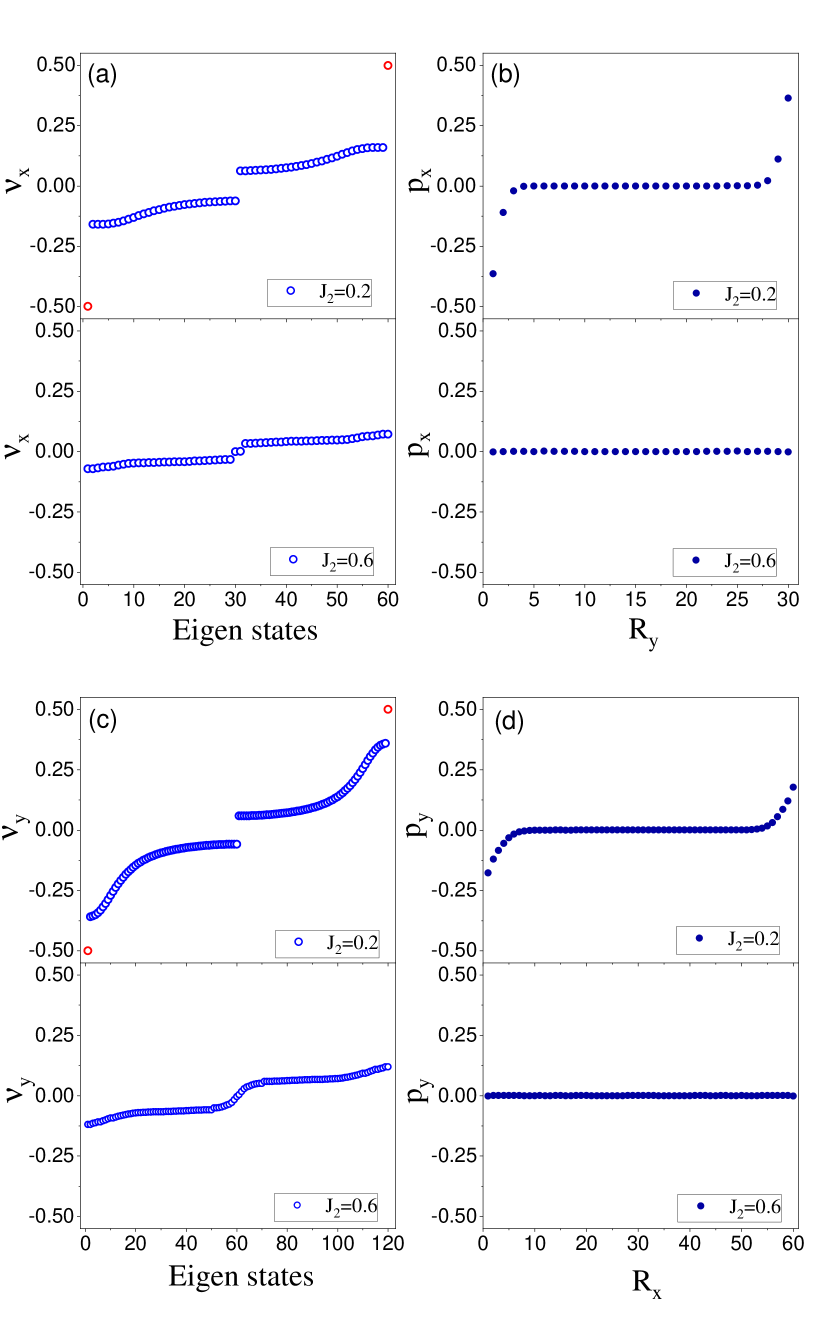
Figure 7: Wannier values and edge polarization before ($J_{2}=0.2$) and after ($J_{2}=0.6$) the topological phase transition. (a) $\nu_{x}$ for different eigen states, (b) edge polarization $p_{x}$ along $R_{y}$, (c) $\nu_{y}$ for different eigen states, (d) edge polarization $p_{y}$ along $R_{x}$. Other parameters are $\gamma_{x}=0.8,\gamma_{y}=0.5.$ Here the red circles in the upper panel of (a) and (c) are used to stress the two isolated topological modes with quantized Wannier center one half.

Second, the edge gap close-reopen process is a topological phase transition. Note that the gap closes at two different $k_{x}$ points. Since the real phase transition occurs at the sample’s boundaries, we focus on the edge spectrum and ignore the Wannier bands at this point. In order to explicitly show the phase transition, we employ several signatures including quadrupole moment $q_{xy}$, fractional corner charges, and quantized edge polarizations. We compare the variation of these signatures before and after the edge spectrum closing point to ensure the occurrence of the topological phase transition. The calculated $q_{xy}$ jumps from $q_{xy}=1/2$ to $q_{xy}=0$ (Fig. 6(c)), indicating that the edge spectrum gap close-reopen process drives the quadrupole insulator from a topological non-trivial phase to a trivial phase. This quadrupole moment jump is associated with the disappearance of both the zero-energy corner modes (Fig. 6(a)) and the fractional corner charges (see Fig. 6(d)). Putting in more detailed words, prior to the phase transition point, the system is gapped with zero-energy corner states, as shown in Fig. 6(a). Following the phase transition point, zero-energy corner modes do not appear in the trivial gap, which is consistent with the result of $q_{xy}$. The real-space numerical calculations of $q_{xy}$ prove to be more effective for the characterization of the quadrupole moments compared to the nested Wilson loop. It is clear that this topological phase transition will modify the original phase diagram. In particular, the non-trivial region will shrink, as shown in Fig. 6(b).

The edge polarization $p_{x}^{\mathrm{edge,}\pm y}$ and $p_{y}^{\mathrm{edge,}\pm x}$, together with the states having Wannier values $\pm 1/2$, can also aid in the detection of the topological phase transition. Figure 7 depicts the edge polarizations and Wannier centers of the system at the two sides of the phase transition point. It is evident that for the non-trivial case where non-zero edge polarizations are present, both $p_{x}(R_{y})$ and $p_{y}(R_{x})$ are accompanied by two isolated topological modes with pinned Wannier center $v_{x,y}=\pm 1/2$ (red circles). Note that the edge polarizations slightly penetrate into the bulk bands, yet their integration over half of the lattice width still results in the quantized value of $\pm e/2$. In comparison, for the trivial case where the edge polarization is maintained at zero, the states with the quantized Wannier values disappear.

IV Robust topological quadrupole phases under mirror symmetry breaking

Mirror symmetries play an important role for the quantization of quadrupole moments in the BBH model. It is thus useful to investigate the consequences of mirror symmetry breaking. To this end, we consider a model that breaks mirror symmetries explicitly, as shown in Fig. 8(a). The generalized model is described as follows:

$$H_{3} =H_{0}+\sum_{\mathbf{R}}J_{3}(iC_{\mathbf{R},2}^{\dagger}C_{\mathbf{R},1}-iC_{\mathbf{R},4}^{\dagger}C_{\mathbf{R},3}+\mathrm{H.c.})$$

$$+\sum_{\mathbf{R}}J_{3}(iC_{\mathbf{R},1}^{\dagger}C_{\mathbf{R}+\hat{x},2}+iC_{\mathbf{R},3}^{\dagger}C_{\mathbf{R}+\hat{x},4}+\mathrm{H.c.}),$$ (11)

where $iJ_{3}$ is the imaginary hopping amplitude. For simplicity, we assume the same hopping amplitudes within and between unit cells. Transforming $H_{3}$ into momentum space gives Bloch Hamiltonian:

$$H_{3}({\bf k})=H_{q}({\bf k})+J_{3}\Gamma_{24}-J_{3}(\sin k_{x}\Gamma_{23}-\cos k_{x}\Gamma_{13}).$$ (12)

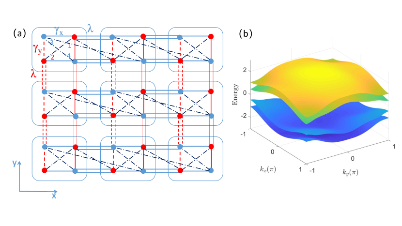
Figure 8: (a) Lattice structure of extended BBH model $H_{3}$. The dashed dark blue lines represent hopping within and between unit cells. Here the artificial asymmetric hopping breaks mirror symmetry. (b) Energy bands corresponding to (a) with parameters fixed at $\gamma_{x}=\gamma_{y}=0.5,$ and $J_{3}=0.3$. The band degeneracy is totally lifted.

The most crucial feature of $H_{3}({\bf k})$ is the breaking of the mirror symmetry, which is evident from our artificial hopping design depicted in Fig. 8(a). Explicitly, we have:

$$\mathcal{M}_{s}H_{3}({\bf k})\mathcal{M}_{s}^{-1}\neq H_{3}(\mathcal{M}_{s}{\bf k}),\ s=x,y.$$ (13)

In this case, the mirror symmetry operators are $\mathcal{M}_{x}=\tau_{1}\sigma_{3},\ \mathcal{M}_{y}=\tau_{1}\sigma_{1}.$ The rotation symmetry $C_{2}=\mathcal{M}_{x}\mathcal{M}_{y}$ of $H_{3}({\bf k})$ is preserved, which allows for well-defined quadrupole moments in the vanishing total bulk polarization BBH17prb . Note that chiral and time-reversal symmetries $\mathcal{C}$ and $\mathcal{T}$ are both absent, thus the discrepancy between the edge spectrum and the Wannier bands also occurs here. Due to the only preserved particle-hole symmetry, the system is categorized into the $D$ class, with a classification of $\mathbb{Z}$ in 2D. It is evident from the numerical result in Fig. 8(b) that the band degeneracy is totally lifted.

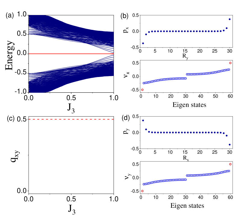
Figure 9: (a) Energy spectrum as function of parameter $J_{3}$. (b) Edge polarization $p_{x}$ along $R_{y}$ (the upper panel) and Wannier center $\nu_{x}$ for different eigen states (the lower panel). (c) Numerically calculated $q_{xy}$ corresponding to (a) panel. (d) Edge polarization $p_{y}$ along $R_{x}$ (the upper panel) and Wannier center $\nu_{y}$ for different eigen states (the lower panel). Other parameters are fixed at $\gamma_{x}=\gamma_{y}=0.5,$ and $J_{3}=0.2$. Here we set system size $L_{x}\times L_{y}=40\times 40$ with periodic boundary for the calculations of $q_{xy}$. Here the red circles in the lower panel of (b) and (d) are used to stress the two isolated topological modes with quantized Wannier center one half.

A crucial result of the generalized model $H_{3}({\bf k})$ is the persistence of the topological quadrupole phases despite the breakdown of the mirror symmetries. In the original BBH model Benalcazar17Science ; BBH17prb , the quantization of the quadrupole moments is protected by the combination of the mirror symmetries ($H_{3}({\bf k})$ does not respect $C_{4}$ symmetry). In the $H_{3}({\bf k})$ model, the robustness of topological quadrupole phases can be demonstrated in several ways. First, it is always valid to calculate quadrupole moments $q_{xy}$. In Fig. 9(c), the numerical results indeed show that for the existing parameters, $q_{xy}$ quantizes at $1/2$ for increasing $J_{3}$. Due to the lack of mirror symmetries, the Wannier sector polarization ${\bf p}^{\nu}$, however, is not quantized. Second, zero-energy corner modes are present. The red line in the spectrum of Fig. 9(a) indicates four-fold degenerate zero-energy modes whose wave functions are sharply localized at the corners of the sample. Moreover, the corner charges are quantized at $\pm e/2$. Third, we found that non-trivial quadrupole phases also correspond to quantized edge polarizations. The lower panels of Figs. 9(b) and 9(d) show that the two topological states located on the edge exhibit half-integer Wannier values, while other states are distributed over the bulk. The edge polarization $p_{x}(R_{y})$ (or $p_{y}(R_{x})$) has a non-zero value close to the edge of the sample. Despite not being highly distributed at the edge sites, the integrated polarization over half of the lattice width still results in the quantized edge polarization of $p_{x}^{\mathrm{edge},\pm y}=\pm e/2$ ($p_{y}^{\mathrm{edge},\pm x}=\pm e/2$). The above observations unambiguously determine the presence of the topological quadrupole phases.

The robustness of $q_{xy}$ under mirror-symmetry breaking can be explained as follows. Although mirror symmetry is used to construct the topological quadrupole insulators, its protection is not necessary for their existence. Once the mirror symmetry is broken, the robust states located at the corners still remain Langbehn17prl ; Trifunovic19prx , and more generally, the existence of corner modes even does not require crystalline symmetry zhang19arxiv ; You2019arXiv . The corner states are associated with the quantized corner charges $\pm e/2$, and cannot be changed adiabatically. This may consequently account for the quantization of $q_{xy}$.

V Quantized quadrupole moments against disorders

In this section, we investigate the disorder effect on the BBH model. Essentially, the topological quadrupole insulator is a topological crystalline insulator, and the presence of disorder can subsequently test the robustness of the topological phase. Furthermore, the involvement of the disorder may induce more interesting topological phases, such as the topological Anderson insulators LiJian09prl .

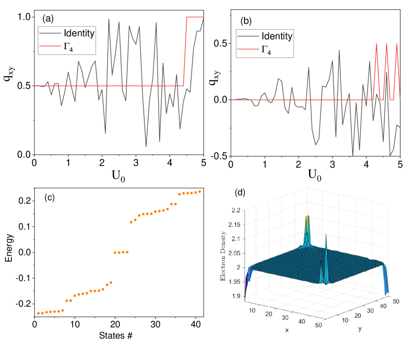
Figure 10: Quadrupole moments in the presence of disorder. Upper panels (a) and (b) plot quadrupole moments $q_{xy}$ as functions of disorder strength $U_{0}$. In topological nontrivial case $\gamma_{x}=0.8$, $\gamma_{y}=0.5$ and trivial case with $\gamma_{x}=1.5$, $\gamma_{y}=0.5$. In panels (a,b) we use periodic boundary condition. (c) Eigen states and (d) electron charge density in the presence of $\Gamma_{4}$ type disorder with strength $U_{0}=3.0$ for the nontrivial case $\gamma_{x}=0.8$, $\gamma_{y}=0.5$. In panels (c,d) we use open boundary condition. The system size is $L_{x}\times L_{y}=50\times 50$, and we only take one disorder configuration for all.

We first consider a simple on-site type of disorder of the form $V_{\mathrm{dis}}=V({\bf R})I_{4\times 4}$ at each lattice site ${\bf R}$. Here $I_{4\times 4}$ is an identity matrix and the random onsite potential, $V({\bf R})$, distributes uniformly in the interval $[-U_{0}/2,U_{0}/2]$ for disorder strength $U_{0}$. Figure 10 shows that for relatively small $U_{0}$ values, the quadrupole moments $q_{xy}$ are well-quantized. This is a reasonable observation as the disorder is weak and can be considered as a series of small perturbations. In addition, for large $U_{0}$ (compared to the bulk gap), $q_{xy}$ exhibits a highly fluctuating trend. If we take the averages across the disorder, the situation improves. More specifically, the quantization of the quadrupole moments recovers under the condition of “averaged mirror symmetry” Benalcazar17Science . However, for much larger values of $U_{0}$, maintaining the quantization of $q_{xy}$ proves impossible.

An interesting phenomenon is observed when we consider another type of disorder, namely, the hopping disorder of the form $V({\bf R})\Gamma_{4}$. Fig. 10 presents the specific parameter configuration used for this case. Results show that the quadrupole moments are well-quantized, regardless of the large disorder strength and lack of disorder average. The quantization of the quadrupole moments is demonstrated by the zero-energy corner modes in the bulk gap (Fig. 10(c)) and the quantized corner charges $\pm e/2$ (Fig. 10(d)). This robustness may be explained as follows. From a 1D point of view, the BBH model can be decomposed into two uncoupled SSH models along the $x$ and $y$ directions. Expressed in terms of $\Gamma$ matrices, the $V({\bf R})\Gamma_{4}$-type disorder respects the chiral symmetry of the SSH model along the $x$ direction. Thus, the topology of each SSH model is still well-defined, regardless of the presence of such a strong disorder Shem14prl . As the disorder strength approaches infinity, we find that the disorder effect dominates and the system becomes trivial. The phase transition from a non-trivial to trivial phase occurs (Fig. 10(a)) and the phase diagram is modified. Interestingly, the high-order topological Anderson-type phase can also appear due to the $\Gamma_{4}$-type disorder LiCA19 . As the central theme of this paper is the quantization of quadrupole moments, here we just focus on the robustness of $q_{xy}$, which remains even under the strong $\Gamma_{4}$ type of disorder where crystalline symmetry is broken down.

VI discussion and conclusions

On the one hand, non-spatial symmetries are not necessary to protect quantization of quadrupole moments, while several generalized models demonstrating that non-spatial symmetry breaking can lead to richer topological phases in the system. On the other hand, although the BBH model is constructed based on a combination of mirror symmetries, when mirror symmetry is broken the quantized quadrupole moments and topologically protected states located at the corners still remain. Thus, the underlying roles played by different symmetries within higher multipole insulators should be further investigated in order to determine their specific impacts on the system.

In summary, we investigate the topological quadrupole phases and consequences of symmetry breaking in the generalized BBH models. We summarize the properties of several generalized models (including the original BBH model) in Table 1. Results from the symmetry analysis indicate that only $C_{2}$ symmetry (inversion symmetry) is required to ensure well-defined quadrupole moments, and quantized quadrupole moments $q_{xy}$ can persist even when mirror symmetry is broken. Besides, we note that nested Wilson loop approach is not suitable to characterize the high-order topology of the generalized models and the topological equivalence between Wannier bands and edge spectrum could be lost; Interestingly, both the quantized quadrupole moments and the topologically protected boundary signatures continue to exist despite the presence of a unique type of disorder. Our results may give a clue to search for more ‘robust’ topological invariant of high-order topological phases.

Table 1: Symmetries and properties of the quantized quadrupole insulator models.

	$\mathcal{M}_{x}$	$\mathcal{M}_{y}$	$C_{2}$	$C_{4}$	$\mathcal{C}$	$\mathcal{\mathcal{T}}$	$\mathcal{P}$	$q_{xy}=0,1/2$	Quantized $p^{\mathrm{edge}}$
$H_{0}({\bf k})$	$\checkmark$	$\checkmark$	$\checkmark$	$\checkmark$	$\checkmark$	$\checkmark$	$\checkmark$	$\checkmark$	$\checkmark$
$H_{1}({\bf k})$	$\checkmark$	$\checkmark$	$\checkmark$	$\checkmark$	$\times$	$\checkmark$	$\times$	$\checkmark$	$\checkmark$
$H_{2}({\bf k})$	$\checkmark$	$\checkmark$	$\checkmark$	$\times$	$\times$	$\times$	$\checkmark$	$\checkmark$	$\checkmark$
$H_{3}({\bf k})$	$\times$	$\times$	$\checkmark$	$\times$	$\times$	$\times$	$\checkmark$	$\checkmark$	$\checkmark$

VII Acknowledgments

C.-A. Li thanks B. Fu, Z.-A. Hu, J. Li, and S.-Q. Shen for helpful discussions, and acknowledges H.-Z Lu at SUSTech. China for hospitality at the initial stage of this project. This work is supported by foundation of Westlake University and the Natural Science Foundation of Zhejiang Province under Grant No. Q20A04005.

Appendix A The effective model

In this appendix, we derive an effective Hamiltonian from BBH model. For the chosen parameters, the bulk gap of BBH model closes at $(\pi,\pi)$ point when $\gamma_{x}=\gamma_{y}=1$. Expanding Eq. (4) around this gap closing point to the second order, we have an effective model

$$H_{\mathrm{eff}}({\bf k}) =\left(\begin{array}[]{cc}0&Q\\ Q^{\dagger}&0\end{array}\right),$$ (16)

$$Q \equiv-m_{x}\sigma_{0}-ik_{x}\sigma_{3}-im_{y}\sigma_{2}-ik_{y}\sigma_{1},$$ (17)

where $m_{x}\equiv 1-\gamma_{x}-k_{x}^{2}/2$, and $m_{y}\equiv 1-\gamma_{y}-k_{y}^{2}/2$. Note that this effective Hamiltonian inherits all symmetries of the original BBH model. After proper rotation of gamma matrices, we arrive at

$$H_{\mathrm{eff}}({\bf k})=m_{x}\beta+\alpha\cdot{\bf p},$$ (18)

where the Dirac matrices are defined as $\beta=\tau_{3}\sigma_{0},$ and $\alpha_{i}=\tau_{1}\sigma_{i}.$ The “momentums” in Eq. (18) are defined as

$${\bf p}\equiv(k_{y},m_{y},k_{x}).$$ (19)

Here we recover the fact that this effective model Eq. (18) is exactly Dirac equation in two dimensions SQS , whereas one of the momentums is replaced by mass term $m_{y}$. Tracing back the relation between $\Gamma_{i}$ matrices before rotation and $\{\beta,{\bf\alpha}\}$ Dirac matrices in Eq. (18), we find that $\Gamma_{4}\rightarrow\beta$. This means that the disorder of the form $V({\bf R})\Gamma_{4}$ modifies the mass term of Dirac Hamiltonian  (18). Besides, it explains why the quadrupole is still quantized when strong disorder is applied, as shown in Fig. 10, to some extent.

Actually, Eq. (18) describes the same physics as quantum spin Hall insulator with an anisotropic edge gap term. This point would be transparent if the Dirac matrices are rotated by a unitary transformation

$$\left(\begin{array}[]{c}\alpha^{\prime}_{2}\\ \beta^{\prime}\end{array}\right)=\frac{1}{\sqrt{2}}\left(\begin{array}[]{cc}1&-1\\ 1&1\end{array}\right)\left(\begin{array}[]{c}\alpha_{2}\\ \beta\end{array}\right).$$ (20)

For simplicity, let us set $\gamma_{x}=\gamma_{y}=\gamma$. With the help of Eq. (20), the effective model is transformed to

$$H_{\mathrm{eff}}({\bf k}) =m({\bf k})\beta^{\prime}+k_{x}\alpha_{3}+k_{y}\alpha_{1}+\Delta({\bf k})\alpha^{\prime}_{2},$$ (21)

$$m({\bf k}) \equiv\left[\sqrt{2}(1-\gamma)-\frac{k^{2}}{2\sqrt{2}}\right],\Delta({\bf k})\equiv\frac{k_{x}^{2}-k_{y}^{2}}{2\sqrt{2}}.$$ (22)

From the mass term $m({\bf k})$, the system is topologically nontrivial when $\gamma<1$, which is consistent with BBH model. Note that the Dirac matrices after rotation still obey Clifford algebra. If $\Delta({\bf k})=0$, which is only satisfied if $k_{x}^{2}=k_{y}^{2}$, the effective Hamiltonian describes quantum spin Hall insulator. Generally, $\Delta({\bf k})$ acts as a mass term to gap helical edge modes as it anticommutes with other Dirac matrices in the Eq. (21), and it creates a domain wall profile since it changes sign at adjacent two edges. In this sense, the BBH model is equivalent to a quantum spin Hall insulator with an anisotropic edge gap term.

Appendix B Calculation details

In this appendix, we show the details about the calculation of nested Wilson loop approach, edge polarization, and etc. Benalcazar17Science ; BBH17prb .

B.1 Wannier bands

The nested Wilson loop approach is based on Wilson loop, thus let us start with the construction of Wilson loop. The Wilson loop operator parallel to the $y$ direction is constructed as

$$\hat{P}_{y,{\bf k}}=P_{N_{y}\delta k_{y}+k_{y}}P_{(N_{y}-1)\delta k_{y}+k_{y}}\cdots P_{\delta k_{y}+k_{y}}P_{k_{y}},$$ (23)

where each projection operator is defined as $P_{m\delta k_{y}+k_{y}}\equiv\sum_{n\in N_{\mathrm{occ}}}|u_{k_{x},m\delta k_{y}+k_{y}}^{n}\rangle\langle u_{k_{x},m\delta k_{y}+k_{y}}^{n}|$ with $|u_{k_{x},m\delta k_{y}+k_{y}}^{n}\rangle$ being the $n$-th eigen state of occupied bands at point $(k_{x},m\delta k_{y}+k_{y})$, and $m$ is an integer taking values from $\{1,2,\cdots,N_{y}\}$. The projection method can avoid the arbitrary phase problem in numerical realizations. Here $N_{y}$ is the number of unit cells, $n$ is the band index, and $N_{\mathrm{occ}}$ is the number of occupied bands. Note that $\hat{P}_{y,{\bf k}}$ has dimension of $N$ now with $N$ being the total bands number. After projection onto the occupied bands at base point ${\bf k}$, there is $N_{\mathrm{occ}}\times N_{\mathrm{occ}}$ matrix $\mathcal{W}_{y,{\bf k}}$ that defines a Wannier Hamiltonian $H_{\mathcal{W}_{y}}({\bf k})$ from the relation $\mathcal{W}_{y,{\bf k}}=\exp[iH_{\mathcal{W}_{y}}({\bf k})]$. The eigen values of $H_{\mathcal{W}_{y}}({\bf k})$ give the Wannier bands $2\pi\nu_{y}(k_{x})$ associated with eigen states $|\nu_{y,{\bf k}}^{j}\rangle$, $j\in\{1,2,\cdots,N_{\mathrm{occ}}\}$. Similar procedure is applicable for the construction of $\mathcal{W}_{x,{\bf k}}$.

B.2 Wannier sector polarization

These Wannier bands can carry their own topology and have associated Berry phases. If the Wannier bands are gapped, then one can chose a Wannier sector and construct nested Wilson loop $\mathcal{\widetilde{W}}_{x,k_{y}}$ by the similar projection procedures as before, which gives rise to Wannier sector polarization $p_{x}^{v_{y}}$. To this end, we need to define the Wannier basis

$$|w_{y,{\bf k}}^{\ell}\rangle=\sum_{n}^{N_{\mathrm{occ}}}|u_{{\bf k}}^{n}\rangle[\nu_{y,{\bf k}}^{\ell}]^{n},$$ (24)

where $\ell$ takes value from the set $\{1,2,\cdots,N_{\mathrm{ws}}\}$, and $N_{\mathrm{ws}}$ is the dimension of chosen Wannier sector. Here $[\nu_{y,{\bf k}}^{\ell}]^{n}$ is the $n$-th component of eigen state $|\nu_{y,{\bf k}}^{\ell}\rangle$. The nested Wilson loop operator parallel along the $x$ direction is constructed as

$$\hat{\mathcal{P}}_{x,{\bf k}}=\mathcal{P}_{N_{x}\delta k_{x}+k_{x}}\mathcal{P}_{(N_{x}-1)\delta k_{x}+k_{x}}\cdots\mathcal{P}_{\delta k_{x}+k_{x}}\mathcal{P}_{k_{x}},$$ (25)

where each projection operator is defined as $\mathcal{P}_{q\delta k_{x}+k_{x}}\equiv\sum_{\ell=1}^{N_{\mathrm{ws}}}|w_{y,q\delta k_{x}+k_{x},k_{y}}^{\ell}\rangle\langle w_{y,q\delta k_{x}+k_{x},k_{y}}^{\ell}|$ where $q$ is also an integer taking values from the set $\{1,2,\cdots,N_{x}\}$. Note that $\hat{\mathcal{P}}_{x,{\bf k}}$ also has dimension of $N$ now. After projection onto the Wannier basis of chosen sector, there is $N_{\mathrm{ws}}\times N_{\mathrm{ws}}$ matrix $\mathcal{\widetilde{W}}_{x,k_{y}}$ that defines a nested Wilson loop. The polarization of Wannier bands is given as

$$p_{x}^{\nu_{y}}=\frac{1}{2\pi iN_{y}}\sum_{k_{y}}\log\det\mathcal{\widetilde{W}}_{x,k_{y}}.$$ (26)

Similar procedure can be carried out for the construction of $p_{y}^{\nu_{x}}$.

B.3 Edge polarization

The edge polarization is exhibited on ribbon samples with finite width but infinite length BBH17prb . It is a useful signature to exhibit high-order topology in quadrupole insulators. Let us assume the ribbon is infinite along the $x$ direction. First, we treat the width along $y$ as inner degree of freedom and get Wannier band $v_{k_{x}}^{s}$using the projection method described as above. The associated wave functions are $|\nu_{k_{x}}^{s}\rangle$ where $s\in\{1,2,\cdots,N_{\mathrm{tot}}\}$ where $N_{\mathrm{tot}}=N_{y}\times N_{\mathrm{occ}}$. Second, we construct hybrid Wannier function as

$$|\Psi_{R_{x}}^{s}\rangle=\frac{1}{\sqrt{N_{x}}}\sum_{k_{x}}\sum_{n=1}^{N_{\mathrm{tot}}}[v_{k_{x}}^{s}]^{n}e^{-ik_{x}R_{x}}\varUpsilon_{n,k_{x}}^{\dagger}|0\rangle,$$ (27)

where $\varUpsilon_{n,k_{x}}$ is the basis that diagonalizes the Hamiltonian. One can check that $|\Psi_{R_{x}}^{s}\rangle$ is a complete basis such that $\langle\Psi_{R_{x}}^{s}|\Psi_{R_{x}}^{s^{\prime}}\rangle=\delta_{ss^{\prime}}.$ Third, we consider the probability distribution of the Wannier function along the $y$ direction

$$\rho^{s}(R_{y}) =\sum_{R^{\prime}_{x},\zeta}\langle\Psi_{R_{x}}^{s}|\phi_{R_{x}^{{}^{\prime}}}^{R_{y,\zeta}}\rangle\langle\phi_{R_{x}^{{}^{\prime}}}^{R_{y,\zeta}}|\Psi_{R_{x}}^{s}\rangle,$$

$$|\phi_{R_{x}^{{}^{\prime}}}^{R_{y,\zeta}}\rangle =\sum_{k_{x}}e^{-ik_{x}R_{x}^{{}^{\prime}}}C_{k_{x},R_{y},\zeta}^{\dagger}|0\rangle,$$ (28)

where $\zeta$ denotes the inner degree of freedom at each unit cell. Finally, the edge polarization along the $x$ direction is

$$p_{x}(R_{y})=\sum_{s=1}^{N_{\mathrm{tot}}}\rho^{s}(R_{y})v_{k_{x}}^{s}.$$ (29)

The total edge polarization $p_{x}^{\mathrm{edge}}$ is defined as summation of $p_{x}(R_{y})$ over half of the width along the $y$ direction, for example

$$p_{x}^{\mathrm{edge,}-y}=\sum_{R_{y}=1}^{N_{y}/2}p_{x}(R_{y}).$$ (30)

B.4 Corner charges

The corner charge is also a direct signature of high-order topology of quadrupole insulators. The local charge density is

$$\rho(R_{x},R_{y})\equiv e\sum_{n=1}^{N_{\mathrm{occ}}}\sum_{\zeta=1}^{4}\left|u^{n}(R_{x},R_{y},\zeta)\right|^{2},$$ (31)

where $u^{n}(R_{x},R_{y},\zeta)$ is the component of $n$-th eigen state $|u^{n}\rangle$. The corner charge is defined as the summation of charge density over a quarter of the sample, for instance,

$$Q^{\mathrm{corner,-x,-y}}=\sum_{R_{x}=1}^{N_{x}/2}\sum_{R_{y}=1}^{N_{y}/2}[\rho(R_{x},R_{y})-2e].$$ (32)

Note that here we need to eliminate contributions from the atomic charge $2e$.

B.5 Quadrupole moments

Classically, the quadrupole moments are defined as

$$q_{ij}=\int d^{3}r\rho(r)r_{i}r_{j},$$ (33)

where $\rho(r)$ is the charge density. The quadrupole moments will manifest observable electromagnetic properties such as corner charges. BBH proposed quantum mechanical crystalline insulator that holds only bulk quadrupole moments, and the defining constraint of the quadrupole insulator is

$$q_{xy}=|p_{x}^{\mathrm{edge}}|=|p_{y}^{\mathrm{edge}}|=|Q^{\mathrm{corner}}|.$$ (34)

In the presence of certain symmetries, the quadrupole moments will be quantized, and they are related to Wannier sector polarizations as

$$q_{xy}\overset{\mathcal{M}_{x},\mathcal{M}_{y}}{=}2p_{x}^{\nu_{y}^{-}}p_{y}^{\nu_{x}^{-}}.$$ (35)

B.6 Phases of BBH model

The BBH model Eq. (4) is a concrete minimal model that holds quantized bulk quadrupole moments. Its bulk bands are gapped unless $\gamma_{s}/\lambda=\pm 1$ ($s=x,y$). Hence it is an insulator at half-filling. The model gives rise to topological quadrupole moments protected by mirror symmetries in principle. The non-spatial symmetries preserved are chiral symmetry, time-reversal symmetry, and particle-hole symmetry, although they are not necessarily needed to quantize quadrupole moments. The topological phase in electric quadrupole insulators is characterized by quantized quadrupole moments $q_{xy}=0,1/2$, which induce corner charge $Q^{\mathrm{corner}}$ and edge polarization $p^{\mathrm{edge}}$ of its equal magnitude. Explicitly, the quantized quadrupole moments are formulated via the nested Wilson loops approach. Sitting on the basis that Wannier bands and boundary spectrum are topologically equivalent, the topological quadrupole phase is characterized by Wannier sector polarization ${\bf p}^{\nu}\equiv(p_{y}^{\nu_{x}^{-}},p_{x}^{\nu_{y}^{-}})$. The nontrivial topological quadrupole phase constrains parameter region $|\gamma_{s}/\lambda|<1$ for $s=x,y$.

References

- (1) R. Resta, Macroscopic polarization in crystalline dielectrics: the geometric phase approach, Rev. Mod. Phys. 66, 899 (1994).
- (2) R. Resta, Quantum-mechanical position operator in extended systems, Phys. Rev. Lett. 80, 1800 (1998).
- (3) R. D. King-Smith and D. Vanderbilt, Theory of polarization of crystalline solids, Phys. Rev. B 47, 1651 (1993).
- (4) D. Xiao, Ming-Che Chang, and Qian Niu, Berry phase effects on electronic properties, Rev. Mod. Phys. 82, 1959 (2010).
- (5) M. Z. Hasan and C. L. Kane, Colloquium: Topological insulators, Rev. Mod. Phys. 82, 3045 (2010).
- (6) X.-L. Qi and S.-C. Zhang, Topological insulators and superconductors, Rev. Mod. Phys. 83, 1057 (2011).
- (7) S.-Q. Shen, Topological Insulators: Dirac Equation in Condensed Matter, 2nd ed. (Springer, Singapore, 2017).
- (8) B. A. Bernevig and T. L. Hughes, Topological insulators and topological superconductors (Princeton University Press, 2013).
- (9) D. J. Thouless, Quantization of particle transport, Phys. Rev. B 27, 6083 (1983).
- (10) L. Fu and C. L. Kane, Time reversal polarization and a adiabatic spin pump, Phys. Rev. B 74, 195312 (2006).
- (11) W. P. Su, J. R. Schrieffer, and A. J. Heeger, Solitons in polyacetylene, Phys. Rev. Lett. 42, 1698 (1979).
- (12) W. A. Benalcazar, B. A. Bernevig, and T. L. Hughes, Quantized electric multipole insulators, Science 357, 61 (2017).
- (13) W. A. Benalcazar, B. A. Bernevig, and T. L. Hughes, Electric multipole moments, topological multipole moment pumping, and chiral hinge states in crystalline insulators, Phys. Rev. B 96, 245115 (2017).
- (14) L. Trifunovic and P. W. Brouwer, Higher-order bulk-boundary correspondence for topological crystalline phases, Phys. Rev. X 9, 011012 (2019).
- (15) F. Schindler, A. M. Cook, M. G. Vergniory, Z. Wang, S. S. P. Parkin, B. A. Bernevig, and T. Neupert, Higher-order topological insulators, Science Advances 4 6 (2018).
- (16) J. Langbehn, Y. Peng, L. Trifunovic, F. von Oppen, and P. W. Brouwer, Reflection-symmetric second-order oopological insulators and superconductors, Phys. Rev. Lett. 119, 246401 (2017).
- (17) E. Khalaf, Higher-order topological insulators and superconductors protected by inversion symmetry, Phys. Rev. B 97, 205136 (2018).
- (18) Z. Song, Z. Fang, and C. Fang, (d-2) -dimensional edge states of rotation symmetry protected topological states, Phys. Rev. Lett. 119, 246402 (2017).
- (19) M. Geier, L. Trifunovic, M. Hoskam, and P. W. Brouwer, Second-order topological insulators and superconductors with an order-two crystalline symmetry, Phys. Rev. B 97, 205135 (2018).
- (20) I. Petrides and O. Zilberberg, (2019), arXiv:1911.08461 [cond-mat.mes-hall].
- (21) Z. Wang, B. J. Wieder, J. Li, B. Yan, and B. A. Bernevig, Higher-order topology, monopole nodal lines, and the origin of large Fermi arcs in transition metal dichalcogenides (), Phys. Rev. Lett. 123, 186401 (2019).
- (22) F. Schindler, Z. Wang, M. G. Vergniory, A. M. Cook, A. Murani, S. Sengupta, A. Y. Kasumov, R. Deblock, S. Jeon, I. Drozdov, H. Bouchiat, S. Gueon, A. Yazdani, B. A. Bernevig, and T. Neupert, Higher-order topology in bismuth, Nat. Phys. 14, 918 (2018).
- (23) M. Serra-Garcia, V. Peri, R. Sustrunk, O. R. Bilal, T. Larsen, L. G. Villanueva, and S. D. Huber, Observation of a phononic quadrupole topological insulator, Nature 555, 342 (2018).
- (24) C. W. Peterson, W. A. Benalcazar, T. L. Hughes, and G. Bahl, A quantized microwave quadrupole insulator with topologically protected corner states, Nature 555, 346 (2018).
- (25) S. Franca, J. van den Brink, and I. C. Fulga, An anomalous higher-order topological insulator, Phys. Rev. B 98, 201114(R) (2018).
- (26) S. Imhof, C. Berger, F. Bayer, J. Brehm, L. W. Molenkamp, T. Kiessling, F. Schindler, C.-H. Lee, M. Greiter, T. Neupert and R. Thomale, Topolectrical-circuit realization of topological corner modes, Nat. Phys. 14, 925 (2018).
- (27) Z. Yan, F. Song, and Z. Wang, Majorana corner modes in a high-temperature platform, Phys. Rev. Lett. 121, 096803 (2018).
- (28) Q. Wang, C.-C. Liu, Y.-M. Lu, and F. Zhang, High-temperature Majorana corner states, Phys. Rev. Lett. 121, 186801 (2018).
- (29) C.-H. Hsu, P. Stano, J. Klinovaja, and D. Loss, Majorana Kramers pairs in higher-order topological insulators, Phys. Rev. Lett. 121, 196801 (2018).
- (30) Y. Volpez, D. Loss, and J. Klinovaja, Second-order topological superconductivity in π -junction Rashba layers, Phys. Rev. Lett. 122, 126402 (2019).
- (31) T. Liu, J. J. He, and F. Nori, Majorana corner states in a two-dimensional magnetic topological insulator on a high-temperature superconductor, Phys. Rev. B 98, 245413 (2018).
- (32) X. Zhu, Tunable Majorana corner states in a two-dimensional second-order topological superconductor induced by magnetic fields, Phys. Rev. B 97, 205134 (2018).
- (33) H. Shapourian, Y. Wang, and S. Ryu, Topological crystalline superconductivity and second-order topological superconductivity in nodal-loop materials, Phys. Rev. B 97, 094508 (2018).
- (34) M. Ezawa, Higher-order topological insulators and semimetals on the breathing kagome and pyrochlore lattices, Phys. Rev. Lett. 120, 026801 (2018).
- (35) R. Okugawa, S. Hayashi, and T. Nakanishi, (2019), arXiv:1907.01153 [cond-mat.mes-hall].
- (36) B. J. Wieder, Z. Wang, J. Cano, X. Dai, L. M. Schoop, B. Bradlyn, and B. A. Bernevig, (2019), arXiv:1908.00016 [cond-mat.mes-hall].
- (37) L. Fu, Topological crystalline insulators, Phys. Rev. Lett. 106, 106802 (2011).
- (38) T. Neupert and F. Schindler, “Topological crystalline insulators,” in Topological Matter: Lectures from the Topological Matter School 2017, edited by D. Bercioux, J. Cayssol, M. G. Vergniory, and M. Reyes Calvo (Springer International Publishing, Cham, 2018) pp. 31– 61.
- (39) J. Kruthoff, J. de Boer, J. van Wezel, C. L. Kane, and R.-J. Slager, Topological classification of crystalline insulators through band structure combinatorics, Phys. Rev. X 7, 041069 (2017)
- (40) A. Yoshida, Y. Otaki, R. Otaki, and T. Fukui, Edge states, corner states, and flat bands in a two-dimensional PT -symmetric system, Phys. Rev. B 100, 125125 (2019).
- (41) E. Khalaf, H. C. Po, A. Vishwanath, and H. Watanabe, Symmetry indicators and anomalous surface states of topological crystalline insulators, Phys. Rev. X 8, 031070 (2018).
- (42) R. Yu, X. L. Qi, A. Bernevig, Z. Fang, and X. Dai, Equivalent expression of topological invariant for band insulators using the non-Abelian Berry connection, Phys. Rev. B 84, 075119 (2011).
- (43) L. Fidkowski, T. S. Jackson, and I. Klich, Model characterization of gapless edge modes of topological insulators using intermediate Brillouin-zone functions, Phys. Rev. Lett. 107, 036601 (2011).
- (44) A. Alexandradinata, X. Dai, and B. A. Bernevig, Wilson-loop characterization of inversion-symmetric topological insulators, Phys. Rev. B 89, 155114 (2014).
- (45) E. Khalaf, W. A. Benalcazar, T. L. Hughes, and R. Queiroz, (2019), arXiv:1908.00011 [cond-mat.meshall].
- (46) Y.-B. Yang, K. Li, L. M. Duan, and Y. Xu, (2019), arXiv:1910.04151 [cond-mat.mes-hall].
- (47) Y.-B. Yang, K. Li, and Y. Xu, (2019), arXiv:1910.14189 [cond-mat.mes-hall].
- (48) A. P. Schnyder, S. Ryu, A. Furusaki, and A. W. W. Ludwig, Classification of topological insulators and superconductors in three spatial dimensions, Phys. Rev. B 78, 195125 (2008).
- (49) C.-K. Chiu, J. C. Y. Teo, A. P. Schnyder, and S. Ryu, Classification of topological quantum matter with symmetries, Rev. Mod. Phys. 88, 035005 (2016).
- (50) B.-H. Chen and D.-W. Chiou, (2017), arXiv:1705.06913 [cond-mat.mes-hall].
- (51) L. Li, Z. Xu, and S. Chen, Topological phases of generalized Su-Schrieffer-Heeger models, Phys. Rev. B 89, 085111 (2014).
- (52) B. Perez-Gonzalez, M. Bello, A. Gomez-Leon, and G. Platero, (2018), arXiv:1802.03973 [cond-mat.meshall].
- (53) B. Kang, K. Shiozaki, and G. Y. Cho, Many-body order parameters for multipoles in solids, Phys. Rev. B 100, 245134 (2019).
- (54) W. A. Wheeler, L. K. Wagner, and T. L. Hughes, Many-body electric multipole operators in extended systems, Phys. Rev. B 100, 245135 (2019).
- (55) B. Roy, (2019), arXiv:1906.10685 [cond-mat.mes-hall].
- (56) S. Ono, L. Trifunovic, and H. Watanabe, Difficulties in operator-based formulation of the bulk quadrupole moment, Phys. Rev. B 100, 245133 (2019).
- (57) C.-A. Li, S.-B. Zhang, and S.-Q. Shen, Hidden edge Dirac point and robust quantum edge transport in InAs/GaSb quantum wells, Phys. Rev. B 97, 045420 (2018).
- (58) R. Skolasinski, D. I. Pikulin, J. Alicea, and M. Wimmer, Robust helical edge transport in quantum spin Hall quantum wells, Phys. Rev. B 98, 201404(R) (2018).
- (59) F. D. M. Haldane, Model for a quantum Hall effect without Landau levels: condensed-matter realization of the "parity anomaly", Phys. Rev. Lett. 61, 2015 (1988).
- (60) S.-B. Zhang and B. Trauzettel, Detection of second-order topological superconductors by Josephson junctions, Phys. Rev. Research 2, 012018(R) (2020).
- (61) Y. You, (2019), arXiv:1908.04299 [cond-mat.str-el].
- (62) J. Li, R.-L. Chu, J. K. Jain, and S.-Q. Shen, Topological Anderson insulator, Phys. Rev. Lett. 102, 136806 (2009).
- (63) I. Mondragon-Shem, T. L. Hughes, J. Song, and E. Prodan, Topological criticality in the chiral-symmetric AIII class at strong disorder, Phys. Rev. Lett. 113, 046802 (2014).
- (64) C.-A. Li, et al., unpublished.