Quantum implementation of an artificial feed-forward neural network

Abstract

Artificial intelligence algorithms largely build on multi-layered neural networks. Coping with their increasing complexity and memory requirements calls for a paradigmatic change in the way these powerful algorithms are run. Quantum computing promises to solve certain tasks much more efficiently than any classical computing machine, and actual quantum processors are now becoming available through cloud access to perform experiments and testing also outside of research labs.
Here we show in practice an experimental realization of an artificial feed-forward neural network implemented on a state-of-art superconducting quantum processor using up to 7 active qubits. The network is made of quantum artificial neurons, which individually display a potential advantage in storage capacity with respect to their classical counterpart, and it is able to carry out an elementary classification task which would be impossible to achieve with a single node. We demonstrate that this network can be equivalently operated either via classical control or in a completely coherent fashion, thus opening the way to hybrid as well as fully quantum solutions for artificial intelligence to be run on near-term intermediate-scale quantum hardware.

I Introduction

The field of artificial intelligence was revolutionized by moving from the simple, single layer perceptron design Rosenblatt (1957) to that of a complete feed-forward neural network (ffNN), constituted by several neurons organized in multiple successive layers Hinton et al. (2006); Hinton (2007). In such artificial neural network designs each constituent neuron receives, as inputs, the outputs (activations) from the neurons in the preceding layer. The advantage of ffNNs with respect to simpler designs such as single layer perceptrons or support vector machines is that they can be used to classify data with relations that cannot be reduced to a separating hyperplane Goodfellow et al. (2016). The present ubiquitous use of artificial intelligence in a wide variety of tasks, ranging from pattern or spoken language recognition to the analysis of large data sets, is mostly due to the discovery that such feed-forward networks can be trained by using well established optimization algorithms Hinton et al. (2006); Hinton (2007); Goodfellow et al. (2016).

Quantum computers hold promise to achieve some form of computing advantage over classical counterparts in the not-so-far future Arute et al. (2019). Indeed, quantum computing has been theoretically shown to offer potentially exponential speedups over traditional computing machines, especially in tasks such as large number factoring, solving linear systems of equations, and data classification Nielsen and Chuang (2004); Shor (1997); Harrow et al. (2009); Lloyd et al. (2014); Rebentrost et al. (2014). More recently, quantum computers have been applied to the field of Artificial Intelligence Schuld et al. (2014); Rebentrost et al. (2018); Lloyd et al. (2013); Biamonte et al. (2017), and recent realizations of artificial neurons Schuld et al. (2015, 2017); Cao et al. (2017); Tacchino et al. (2019) and support vector machines Havlíček et al. (2019); Schuld and Killoran (2019) on real quantum processors, even if limited to simple systems at present, have shown a promising route towards a practical realization of such advantage.

In order to harness the full potentialities that quantum computing may offer to the field of artificial intelligence it is necessary to undergo the passage from single layered to deep feed-forward neural networks Wan et al. (2017); Grant et al. (2018); Cong et al. (2019), which has so greatly expanded the capabilities of artificially intelligent systems to date. Here we propose the architecture of a quantum ffNN and we test it on a state-of-the art 20-qubit IBMQ quantum processor. We start from a hybrid approach combining quantum nodes with classical information feed-forward, obtained via classical control of unitary transformations on qubits. This design realizes a fully general implementation of a ffNN on a quantum processor assisted by classical registers. A minimal 3-node example, specifically designed to carry out a pattern recognition task exceeding the capabilities of a single artificial neuron, is used for a proof-of-principle demonstration on real quantum hardware. We then describe and successfully implement on a 7-qubit register an equivalent fully quantum coherent configuration of the same set-up, which does not involve classical control of the feed-forward links and thus potentially opens the way to the exploration of more complex and classically inaccessible regimes.

The proposed quantum implementation of ffNN offers interesting perspectives on scalability already in the Noisy Intermediate-Scale Quantum (NISQ) Preskill (2018) regime: indeed, the single quantum nodes potentially feature exponential advantage in memory usage, thus allowing to manipulate high-dimensional data structures with intermediate-size quantum registers, in principle. Moreover, the hybrid nature of the ffNN itself suggests a seamless integration with existing classical structures and algorithms for neural network computation and machine learning Mari et al. (2019).

II Design of the hybrid feed-forward neural network

In this section, we outline the general structure of our proposed hybrid ffNN, including a synthetic description of the working principles of single nodes and a more detailed discussion of layer-to-layer connections. While, for the sake of clarity, we will often refer to a specific minimal example with three nodes and two layers, the overall scheme can be generalized to arbitrary feed-forward networks.

II.1 Individual nodes

A ffNN is essentially composed of a set of individual nodes $\{n_{i}\}$, or artificial neurons, arranged in a set of successive layers $\{L_{j}\}$. Information flows through the network in a well defined direction from the input to the output layer, travelling through neuron-neuron connections (i.e. artificial synapses). Each node performs an elementary non-linear operation on the incoming data, whose result is then passed on to one or more nodes in the successive layer.

In their simplest form, individual nodes can be designed to analyze binary-valued inputs. The artificial neurons that we consider here are based on the well known perceptron model Rosenblatt (1957): such computational units analyze information by combining input ($\vec{i}$) and weight ($\vec{w}$) vectors, providing an activation response that depends on their scalar product $\vec{i}\cdot\vec{w}$. In our case, input and weight vectors are assumed to be binary-valued $m$-dimensional arraysMcCulloch and Pitts (1943), i.e.

$$\vec{i}=\begin{pmatrix}i_{0}\\ i_{1}\\ \vdots\\ i_{m-1}\end{pmatrix}\,,\quad\vec{w}=\begin{pmatrix}w_{0}\\ w_{1}\\ \vdots\\ w_{m-1}\end{pmatrix}$$ (1)

where $i_{k},w_{k}\in\{-1,1\}\,\forall k$. The activity of a binary artificial neuron can be implemented on a quantum register of $N=\log_{2}(m)$ qubits Tacchino et al. (2019) by considering the quantum states

$$|\psi_{i}\rangle=\frac{1}{\sqrt{m}}\sum_{j=0}^{m-1}i_{j}|j\rangle\,,\quad|\psi_{w}\rangle=\frac{1}{\sqrt{m}}\sum_{j=0}^{m-1}w_{j}|j\rangle$$ (2)

These encode the corresponding input and weight vectors by effectively exploiting the exponential size of the Hilbert space associated to the quantum register in use. The states of the form presented in Eq. (2) are real equally-weighted (REW) superpositions of all the computational basis states $|j\rangle\in\{|0\ldots 00\rangle;|0\ldots 01\rangle;\ldots,|1\ldots 11\rangle\}$. The quantum procedure carrying out the perceptron-like computation for single artificial neurons can be summarized in three steps Tacchino et al. (2019). First, assuming that the $N$-qubits quantum register is initially in the idle configuration, $|0\rangle^{\otimes N}$, we prepare the quantum state encoding the input vector with a unitary operation $\mathrm{U}_{i}$ such that $|\psi_{i}\rangle=\mathrm{U}_{i}|0\rangle^{\otimes N}$. We then apply the weight factors of vector $\vec{w}$ on the input state by implementing another unitary transformation, $\mathrm{U}_{w}$, subject to the constraint $|1\rangle^{\otimes N}=\mathrm{U}_{w}|\psi_{w}\rangle$. An optimized yet exact implementation of $\mathrm{U}_{i}$ and $\mathrm{U}_{w}$ exploits the close relationship between REW quantum states and the class of hypergraph states Rossi et al. (2013); Tacchino et al. (2019), achieving in the worst case an overall computational complexity which is linear in the size of the classical input, i.e. $O(m)$. After the two unitaries have been performed, it is easily seen that the state of the quantum register is

$$|\phi_{i,w}\rangle=\mathrm{U}_{w}\mathrm{U}_{i}|0\rangle^{\otimes N}=\sum_{j=0}^{m-1}c_{j}|j\rangle$$ (3)

where $c_{m-1}=\langle\psi_{w}|\psi_{i}\rangle=(1/m)\vec{i}\cdot\vec{w}$. Finally, the non-linear activation of the single artificial neuron can be implemented by performing a multi-controlled $\mathrm{NOT}$ gate Nielsen and Chuang (2004) between the encoding register and an ancilla initialized in the initial state $|0\rangle$

$$|\phi_{i,w}\rangle|0\rangle_{a}\rightarrow\sum_{j=0}^{m-2}c_{j}|j\rangle|0\rangle_{a}+c_{m-1}|m-1\rangle|1\rangle_{a}$$ (4)

followed by a final measure of the ancilla in the computational basis. Hence, the output of the quantum artificial neuron is found in the active state $|1\rangle_{a}$ with probability $p(1)=|c_{m-1}|^{2}$.

II.2 Information feed-forward

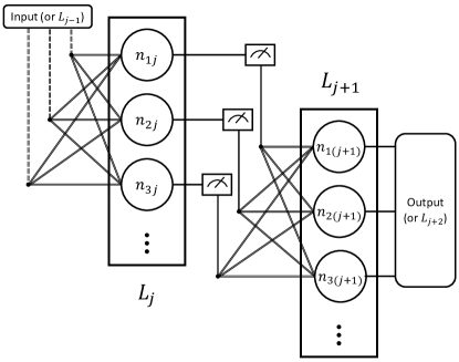
Figure 1: Abstract architecture of a hybrid ffNN. Each layer $L_{j}$ contains an arbitrary number of nodes $\{n_{kj}\}$, which can individually be implemented on a quantum hardware. Upon measurement, information about the activation state of a layer is passed to the following one ($L_{j+1}$) in the form of classical bits controlling quantum operations. Full connectivity between nodes in successive layers is schematically shown, although sparser networks are also possible in principle. The dashed line represents classical inputs from a generic preceding stage, which can be, e.g., a collection of layers up to $L_{j-1}$ or the original input information.

When several copies of the quantum register implementing the artificial neuron model outlined above work in parallel, the respective ancillae, and the result of the measurements performed on them, can be used to feed-forward the information about the input-weight processing to a successive layer. Indeed, let us suppose that a layer $L_{j}$ contains $\ell_{j}$ independent nodes, $\{n_{kj}\}_{k=1}^{\ell_{j}}$, each of them characterized by a weight vector $\vec{w}_{kj}$: in one cycle of operation, every node is provided with a classical input $\vec{i}_{kj}$ (either coming from layer $L_{j-1}$ or directly from the original data set to be analyzed) and, upon measurement, it outputs an activation state $a_{kj}\in\{1,0\}$, chosen according to a probability $p_{kj}(a_{kj}=1)\propto|\vec{i}_{kj}\cdot\vec{w}_{kj}|^{2}$. Assuming for simplicity that the $h$-th neuron $n_{h(j+1)}$ belonging to the $L_{j+1}$ layer collects the outputs of all $\{n_{kj}\}$ nodes, the corresponding binary classical input can be constructed as

$$\vec{i}_{h(j+1)}=\begin{pmatrix}(-1)^{a_{1j}}\\ (-1)^{a_{2j}}\\ \vdots\\ (-1)^{a_{\ell_{j}j}}\end{pmatrix}$$ (5)

Such new input vector can then be used to parametrize the appropriate $\mathrm{U}_{i}$ transformation for the $n_{h(j+1)}$ node. The overall computation can then be constructed by iteratively alternating the unitary quantum computation carried out by single layers with non-linear measurement and feed-forward stages. Notice that the design is totally general in terms of the number of nodes in each layer, the number of connections and the size of the various inputs to individual nodes. Moreover, as the information is formally transferred in the form of classical bits, the same input can easily be manipulated, e.g., by making classical copies to be fed to independent nodes sharing similar connections to the previous layer. An abstract representation of the proposed architecture is shown in Fig. 1.

From the technical point of view, a very natural implementation of the hybrid ffNN architecture onto a quantum processor makes use of classically controlled quantum gates. Independent quantum nodes within the same layer can either be implemented in different quantum registers, and thus computed simultaneously, or run on the same set of qubits, after proper re-initialization and by storing all the observed activation states in different positions of a classical memory register.

II.3 Example: pattern recognition

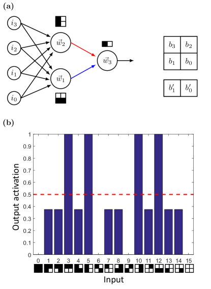
Figure 2: 3-node ffNN for patter recognition. (a) The minimal example of a feed-forward neural network that we analyze in this study accepts four classical binary inputs and features one hidden layer containing two artificial neurons plus one output layer made of a single neuron. Next to each neuron, the ideal shape of the weight vectors achieving the desired recognition of horizontal and vertical lines is shown. The corresponding encoding scheme in terms of black and white pixels is also reported for a generic input/weight binary vector $\vec{b}=(b_{0},\ldots,b_{m})$. (b) Ideal results for the classification of $2\times 2$ pixel images. Notice that the target patterns, corresponding to integer labels $12$, $3$ (horizontal), $10$ and $5$ (vertical) all have $p^{out}=1$, while all others have $p^{out}<0.5$ (threshold shown in red).

The working principles of our proposed hybrid ffNN, including the above technical details, are actually best clarified by describing an explicit example tailored to solve a well defined elementary classification problem. This will also set the stage for the experimental proof-of-principle demonstration on an actual superconducting quantum hardware to be presented in the next section. First, let us recall that binary input and weight vectors can be visually interpreted as images containing black or white square pixels Tacchino et al. (2019): a natural encoding scheme associates, e.g., a white spot to a $i_{j}(w_{j})=-1$ entry in the corresponding input (weight) vector, as shown explicitly in Fig. 2a for the hidden ($m=4$, i.e. $2\times 2$ pixel images) and output ($m=2$, i.e. $2\times 1$ pixel images) layers of a minimal ffNN. Moreover, we can identify any such binary pattern with a unique integer label by considering the equivalent decimal representation of the binary number $\mathtt{b}_{3}\mathtt{b}_{2}\mathtt{b}_{1}\mathtt{b}_{0}$ where $b_{k}=(-1)^{\mathtt{b}_{k}},\,\mathtt{b}_{k}\in\{0,1\}$. The task that we set out to solve with our example ffNN is the following: the network should be able to recognize (i.e., give a positive output activation with sufficiently large probability) whether there exist straight lines in $2\times 2$ pixel images, regardless of the fact that the lines are horizontal or vertical. All the other possible input images should be classified as negative. Notice that, as the data vectors encoding horizontal and vertical lines are orthogonal to each other, there is no single hyperplane separating the four positive states from all other possible input images: therefore, the desired classification cannot be carried out by a single node accepting 4-bit inputs. This behavior of quantum artificial neurons differs from their usual classical counterparts, which cannot correctly classify sets containing opposite vectors Goodfellow et al. (2016). More explicitly, given an input vector $\vec{v}_{1}$ and a weight vector $\vec{w}$, a single quantum neuron would output a value proportional to $|\vec{v}_{1}\cdot\vec{w}|^{2}$, i.e. $\cos^{2}\theta$, where $\theta$ is the angle formed by the two vectors. If we take a second input vector $\vec{v}_{2}\perp\vec{v}_{1}$, the output would be upper bounded by $\sin^{2}\theta$. As the set of patterns that should yield a positive result includes vectors that are orthogonal (those representing horizontal lines are orthogonal to those representing vertical lines) and vectors that are opposite (for instance, the vector corresponding to a vertical line on the left column of a $2\times 2$ pixel image is opposite to the vector corresponding to a vertical line on the right column), it is therefore impossible to find a weight $\vec{w}$ capable of yielding an output activation larger than $0.5$ for all targets in the configuration space. We hereby show that a simple three-node network can accomplish the desired computation. A scheme of such an elementary ffNN is shown in Fig. 2a, where the circles indicate individual artificial neurons, and the vectors $\vec{w}_{i}$ refer to their respective weights. The network features a single hidden layer and a single binary output neuron. On a conceptual level, the functioning of the network can be interpreted as follows: with the a priori choice of weights represented in Fig. 2a, the top quantum neuron of the hidden layer outputs a high activation if the input vector has vertical lines, while the bottom neuron does the same for the case of horizontal lines. The output neuron in the last layer then recognizes whether one of the neurons in the hidden layer has given a positive outcome.

A possible quantum circuit description of the ffNN introduced above, including the classical feed-forward stage between the hidden and the output layer, is provided in Fig. 3a. We assume that each neuron within the hidden layer can accept 4-bit inputs, such that each quantum neuron can be represented on a 2-qubit encoding register plus an ancilla qubit (i.e., $m=4$ and $N=2$ in this case). At the same time, the output neuron takes 2-dimensional inputs coming from the previous layer and provides the global activation state of the network, thus requiring a single qubit ($m=2$, $N=1$) to be encoded. Classical bits are also included to store the intermediate and final results.

Let us call $n_{1}$ and $n_{2}$ the two hidden nodes, which actually accept the same classical input but process it in two different ways. As described at the beginning of this section, each artificial neuron will independently provide, upon measurement, an activation pattern $a_{k}\in\{0,1\}\,(\text{for}\,k=1,2)$, which can be stored in a classical bit $b_{k}$. We denote $p_{k}$ the probability of actually observing a value $a_{k}=1$ from the $k$-th neuron. When such measurement is performed, we set $b_{k}=a_{k}$: as a result, the state of the classical 2-bit register after the quantum computation in the hidden layer has been completed is one of the following

$$[b_{1},b_{2}]=\begin{cases}[0,0]\\ [0,1]\\ [1,0]\\ [1,1]\end{cases}$$ (6)

with probability

$$p([b_{1},b_{2}])=\begin{cases}(1-p_{1})(1-p_{2})\\ (1-p_{1})p_{2}\\ p_{1}(1-p_{2})\\ p_{1}p_{2}\end{cases}$$ (7)

respectively. It is easy to see that feed-forwarding the information contained in the classical register to the output neuron $n_{3}$ corresponds to providing it with one of the classical binary inputs $\vec{i}_{b_{1}b_{2}}$ reading

$$\begin{split}\vec{i}_{00}=\begin{pmatrix}1\\ 1\end{pmatrix},\quad\vec{i}_{01}=\begin{pmatrix}1\\ -1\end{pmatrix}\\ \vec{i}_{10}=\begin{pmatrix}-1\\ 1\end{pmatrix},\quad\vec{i}_{11}=\begin{pmatrix}-1\\ -1\end{pmatrix}\end{split}$$ (8)

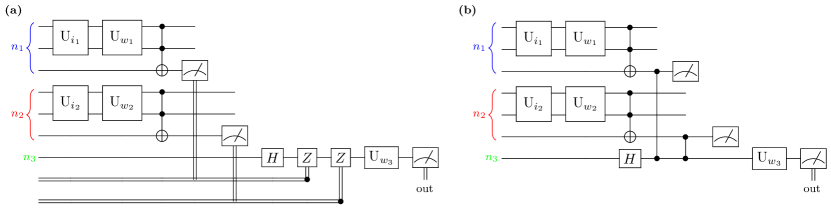
Figure 3: Circuit implementation of a ffNN. (a) Hybrid realization of the feed-forward architecture introduced in Fig. 2 via classical control. (b) Equivalent quantum coherent version using quantum controlled operations.

As shown in Fig. 3a, a straightforward strategy for preparing the corresponding $|\psi_{i}\rangle$ state on the single-qubit register representing $n_{3}$ is by first bringing it from the idle state $|0\rangle$ to the superposition $\sqrt{2}|+\rangle=|0\rangle+|1\rangle$ via a Hadamard ($\mathrm{H}$) gate, and then conditioning the application of two $\mathrm{Z}$ gates (each of them adds a $-1$ phase to the $|1\rangle$ component, if applied) on the two classical bits $[b_{1},b_{2}]$. The resulting quantum state will then be

$$|\psi_{i}\rangle_{n_{3}}=\frac{1}{\sqrt{2}}\left(|0\rangle+(-1)^{b_{1}\oplus b_{2}}|1\rangle\right)$$ (9)

where $a\oplus b$ here denotes the usual bit sum modulo 2. If we now choose, as shown in Fig. 2a, a weight vector $\vec{w}_{3}=(1,-1)$ we obtain $\mathrm{U}_{w_{3}}\equiv\mathrm{H}$. Therefore, the final state of the third neuron reads

$$|\psi_{out}\rangle_{n_{3}}=\begin{cases}|0\rangle\quad&\text{if }b_{1}\oplus b_{2}=0\\ |1\rangle\quad&\text{if }b_{1}\oplus b_{2}=1\end{cases}$$ (10)

The overall probability of observing an active state on the output neuron can be written, in general, as

$$p^{out}=\sum_{[b_{1},b_{2}]}p([b_{1},b_{2}])p(a_{3}=1|[b_{1},b_{2}])$$ (11)

where we employed the usual notation for conditional probabilities and

$$p(a_{3}=1|[b_{1},b_{2}])=|\langle 1|\psi_{out}\rangle_{n_{3}}|^{2}$$ (12)

In our specific case, it is easy to see that, given Eq. (7) and Eq. (10), this reduces to

$$p^{out}=p_{1}(1-p_{2})+(1-p_{1})p_{2}$$ (13)

Since in this elementary example $n_{3}$ is encoded in a single qubit, the final measurement can be performed directly without the need for an additional ancilla. In Fig. 2b we report the exact result for the convolution of Eq. (13): as it can be seen, the ffNN ideally outputs an active state with $p^{out}=1$ for the target horizontal and vertical patterns, while $p^{out}<0.5$ in all other cases.

Before moving forward, it is worth mentioning that the construction of a classically conditioned $\mathrm{U}_{i}$ can always be found also in more general cases, e.g. when the hidden layer contains more than two neurons. In particular, any node encoded on $N$ qubits will be able to accept inputs from $m=2^{N}$ nodes in the previous layer: indeed, each output configuration from the latter will be one of the $2^{m}$ possible bit strings $[b_{1},\ldots,b_{m}]$ that can be used to uniquely identify one of the $2^{m}=2^{2^{N}}$ possible input states, and thus to classically program its preparation.

III Quantum coherent feed-forward

The hybrid feed-forward architecture described so far and realized in a minimal 3-node 2-layer example can also be reformulated in a fully quantum coherent way. As we will show below, and at difference with the hybrid quantum-classical solution, this version always requires all nodes to be implemented simultaneously on a dedicated quantum register, thus making the quantum computation more demanding. At the same time, however, it reduces the necessity to store and process classical bits during intermediate stages. Moreover, fully coherent quantum neural networks offer more opportunities for use on quantum processors, as will be discussed in the final conclusions.

In Fig. 3b we show a fully quantum construction for the ffNN of Fig. 3a. The fundamental reason for the actual equivalence lies in the well known principle of deferred measurement Nielsen and Chuang (2004), stating that in a quantum circuit one can always move a measurement done at an intermediate stage to the end of the computation while replacing classically controlled operations ($\mathrm{O}$) with quantum controlled ones:

$$\Qcircuit@C=1.0em@R=0.0em@!R{&\meter\control\cw\cwx[2]\ctrl{2}\meter\\ =\\ \qw\gate{\mathrm{O}}\qw\gate{\mathrm{O}}\qw\\ }$$

Indeed, assuming that the nodes $n_{1}$ and $n_{2}$ are encoded in parallel and after the operations of the first layer (except the measurement on the ancillae) have been performed, we can write the global state of the total (3+3+1)-qubit network as

$$\begin{split}&\left(r_{n_{1}}|\varphi_{n_{1}}\rangle|0\rangle_{a_{1}}+c_{m-1,n_{1}}|1\ldots 1\rangle_{n_{1}}|1\rangle_{a_{1}}\right)\\ &\otimes\left(r_{n_{2}}|\varphi_{n_{2}}\rangle|0\rangle_{a_{2}}+c_{m-1,n_{2}}|1\ldots 1\rangle_{n_{2}}|1\rangle_{a_{2}}\right)\\ &\otimes|0\rangle_{n_{3}}\end{split}$$ (14)

where $r_{n_{x}}=(1-c_{m-1,n_{x}}^{2})^{1/2}$ and $|\varphi_{n_{x}}\rangle$ contains, for each neuron, all the components other than the one leading to activation, see Eq. (4). Notice that, by construction, $\langle\varphi_{n_{x}}|1\ldots 1\rangle=0$. In the meantime, the $n_{3}$ qubit is brought into the superposition $\sqrt{2}|+\rangle=|0\rangle+|1\rangle$ by applying a single-qubit Hadamard gate, $\mathrm{H}$. Synapses can thereafter be implemented with two $\mathrm{CZ}$ gates, as represented in Fig. 3b. The overall state of the quantum ffNN then becomes

$$\begin{split}&\left(r_{n_{1}}r_{n_{2}}|R_{n_{1}}\rangle|R_{n_{2}}\rangle+c_{n_{1}}c_{n_{2}}|A_{n_{1}}\rangle|A_{n_{2}}\rangle\right)|+\rangle_{n_{3}}\\ &+\left(r_{n_{1}}c_{n_{2}}|R_{n_{1}}\rangle|A_{n_{2}}\rangle+c_{n_{1}}r_{n_{2}}|A_{n_{1}}\rangle|R_{n_{2}}\rangle\right)|-\rangle_{n_{3}}\end{split}$$ (15)

where $c_{n_{x}}$ is a short-hand notation for $c_{m-1,n_{x}}$, and the activated $|A\rangle$ and rest $|R\rangle$ states of $n_{1}$ and $n_{2}$ are explicitly given as

$$\begin{split}|A_{n_{x}}\rangle&=|1\ldots 1\rangle_{n_{x}}|1\rangle_{a_{x}}\\ |R_{n_{x}}\rangle&=|\varphi_{n_{x}}\rangle|0\rangle_{a_{x}}\end{split}$$ (16)

By applying $\mathrm{U}_{w_{3}}\equiv\mathrm{H}$ on $n_{3}$ we obtain an output state

$$\begin{split}&|\psi_{out}\rangle=\\ &\left(r_{n_{1}}r_{n_{2}}|R_{n_{1}}\rangle|R_{n_{2}}\rangle+c_{n_{1}}c_{n_{2}}|A_{n_{1}}\rangle|A_{n_{2}}\rangle\right)|0\rangle_{n_{3}}\\ &+\left(r_{n_{1}}c_{n_{2}}|R_{n_{1}}\rangle|A_{n_{2}}\rangle+c_{n_{1}}r_{n_{2}}|A_{n_{1}}\rangle|R_{n_{2}}\rangle\right)|1\rangle_{n_{3}}\end{split}$$ (17)

It is straightforward to observe at this point that the neurons of the hidden layer can in principle be measured in an activation state $[b_{1},b_{2}]\in\{[0,0],[0,1],[1,0],[1,1]\}$ with probabilities

$$p([b_{1},b_{2}])=\begin{cases}|r_{n_{1}}|^{2}|r_{n_{2}}|^{2}=(1-p_{1})(1-p_{2})\\ |r_{n_{1}}|^{2}|c_{n_{2}}|^{2}=(1-p_{1})p_{2}\\ |c_{n_{1}}|^{2}|r_{n_{2}}|^{2}=p_{1}(1-p_{2})\\ |c_{n_{1}}|^{2}|c_{n_{2}}|^{2}=p_{1}p_{2}\end{cases}$$ (18)

which exactly correspond to the ones reported in Eq. (7). However, as long as we are interested only in the output state of the network, i.e. the activation state $a_{3}$ of $n_{3}$, there is no need to actually perform the final measurements on $n_{1}$ and $n_{2}$: similarly to Eq. (11), we can in fact simply discard the information contained in the variables pertaining to the hidden layer by performing a partial trace operation. This returns a density matrix for the output neuron

$$\rho_{n_{3}}=\operatorname{Tr}_{\{n_{1},n_{2}\}}\left[|\psi_{out}\rangle\langle\psi_{out}|\right]=\begin{pmatrix}1-p^{out}&0\\ 0&p^{out}\end{pmatrix}$$ (19)

which automatically represents the convolution of the hidden nodes, see Eq. (13). It is worth noticing that the role of the partial trace operation has recently been recognized and extensively discussed in the literature as a possible ingredient for a more general theory of quantum neural networks Torrontegui and Garcia-Ripoll (2019); Beer et al. (2019).

To conclude this section, we also point out explicitly that the conversion between the two modes of operation (hybrid vs coherent) of our proposed ffNN architecture goes beyond the specific example presented in this work. Indeed, as mentioned at the end of Sec. II.3, any feed-forward link between successive layers can in general be decomposed in terms of classically controlled operations. Whenever such construction is known, measurement deferral and partial traces can in principle always be employed to obtain the equivalent coherent network, namely by replacing all classical controls with their quantum counterparts and by measuring only the output layer.

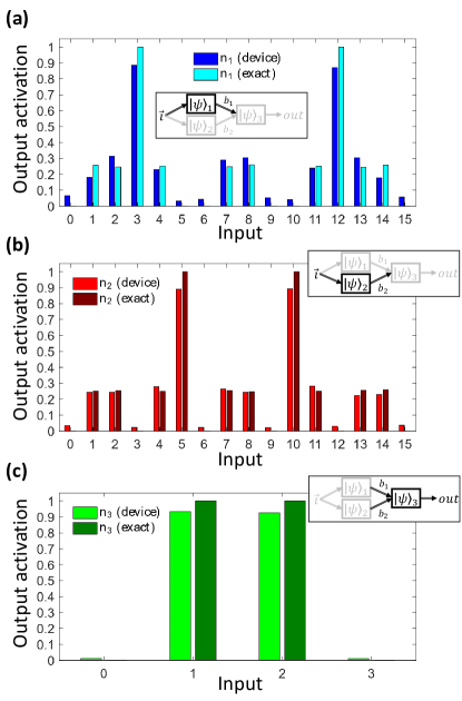
Figure 4: Experimental realization of single nodes on quantum hardware. Single artificial neurons of the ffNN introduced in Fig. 3a implemented on the IBMQ Poughkeepsie superconducting processor and compared with ideal noiseless outcomes computed numerically with the Qiskit qasm_simulator. (a) Neuron $n_{1}$, recognizing horizontal inputs. (b) Neuron $n_{2}$, recognizing vertical inputs. (c) Neuron $n_{3}$, recognizing 2-dimensional inputs with dissimilar entries. Error mitigation is applied to data for $n_{1}$ and $n_{2}$.

IV Experimental realization on a superconducting NISQ processor

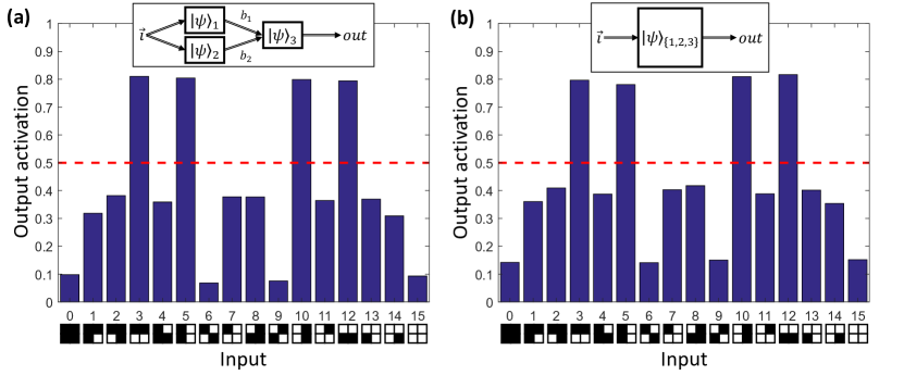
Figure 5: Results for the quantum ffNN classifying horizontal and vertical lines. (a) Classification in the hybrid configuration, applying Eq. (11) to the (error mitigated) experimental outcomes of Fig. 4. (b) Classification in the coherent configuration obtained with a 7-qubit calculation on the IBMQ Poughkeepsie quantum processor (error mitigation is applied). Despite some residual quantitative inaccuracy, all the target patterns are correctly recognized if a threshold $\epsilon=0.5$ (shown in red) is applied to the outcome probabilities both in the hybrid and the coherent versions.

We have implemented the ffNN introduced in Fig. 2 on a real superconducting NISQ processor made available on cloud via the IBM Quantum Experience and programmed using the Qiskit python library et al. (2019). Employing the same device, named IBMQ Poughkeepsie, we realized both the hybrid (Fig. 3a) and the fully coherent (Fig. 3b) configurations, reporting in both cases a remarkable successful completion of all the desired classification tasks.

In Fig. 4a-b we show the results for the 3-qubit simulation of nodes $n_{1}$ and $n_{2}$, respectively corresponding to the first and second set of three qubits in Fig. 3a, from which the probabilities $p_{1}$ and $p_{2}$ can be estimated for all possible input vectors while assuming the weights $\vec{w}_{1}$ and $\vec{w}_{2}$ shown in Fig. 2a. The comparison with ideal results simulated numerically shows an excellent qualitative agreement and a good quantitative match of the outcomes: in particular, notice that each individual node can successfully single out either vertical or horizontal lines, see patterns in Fig. 2b Tacchino et al. (2019). The agreement is naturally better for the simulation of all possible $n_{3}$ circuits, whose results are reported in Fig. 4c: indeed, in this case the probability $p(a_{3}=1|[b_{1},b_{2}])$ can be computed operating on a single qubit. The final outcomes (i.e. $p^{out}$) for the hybrid configuration of the ffNN, reported in Fig. 5a, are then obtained by applying Eq. (11). The latter is used in place of e.g. Eq. (13) in order to avoid introducing unnecessary assumptions or biases in the calculation and to take into account all possible sources of inaccuracy such as, for example, a non exactly zero outcome for $p(a_{3}=1|[0,0])$.

Finally, the experimental results for the fully coherent ffNN configuration are reported in Fig. 5b. These were obtained by running the 7-qubit quantum circuit introduced in Fig. 3b. As it can immediately be appreciated, the outcomes are in good agreement with the corresponding ones in the hybrid version of the ffNN. We stress that such comparison is made non-trivial from the experimental point of view by the fact that, in the fully coherent version, a register of 7 simultaneously active and typically entangled qubits is required. On the contrary, the hybrid solution only requires each individual node to be separately implemented on a 3-qubit quantum register and, provided that the classical outcomes are conveniently stored, such quantum computations can be carried out in dedicated runs, thus avoiding e.g. cross-talks effects. As in the hybrid case, and despite some residual quantitative inaccuracy in the estimation of the activation probabilities, all the possible inputs are classified correctly by the ffNN, with the target horizontal and vertical patterns singled out from all other patterns.

We also mention that raw data from the quantum processor already allow for an accurate classification in both hybrid and coherent configurations. However, the overall quality of the outcomes greatly benefits from the application of simple error mitigation techniques Temme et al. (2017); Li and Benjamin (2017); Klco et al. (2018); Kandala et al. (2019).

V Discussion

In this work we have presented an original architecture to build feed-forward neural networks on universal quantum computing hardware and demonstrated the use of them in NISQ devices. In particular, we have shown how successive layers constituted by artificial neurons and implemented on independent quantum registers can be either connected to each other via classical control operations, thus realizing a hybrid quantum-classical ffNN, or by fully coherent quantum synapses. The necessary degree of non-linearity is achieved in one case via explicit quantum measurement, in the other by a partial trace operation that effectively produces a convolution operation. We stress that our proposed procedure is hardware-independent and therefore it can, in principle, be implemented on any quantum computing machine, e.g. based on superconducting qubits Wendin (2017), trapped-ions based quantum processors Schindler et al. (2013), and photonic components Aspuru-Guzik and Walther (2012); Takeda and Furusawa (2019).

In the present work, we have successfully tested a 3-node implementation of our algorithm applied to an elementary pattern classification task, both in the hybrid and fully coherent configurations. Such proof-of-principle demonstration was achieved on the IBMQ Poughkeepsie superconducting quantum processor by using up to 7 active qubits, and finding a substantial experimental agreement between the two proposed operating modes of the network. These results represent, to the best of our knowledge, one of the largest quantum neural network computation reported to date in terms of the total size of the quantum register. We also notice that the use of quantum artificial neurons as individual nodes gives the prospective advantage of an exponential gain in storage and processing ability: in turn, this confirms that hybrid quantum-classical neural networks could already be able to treat very large input vectors, beyond the capabilities of current systems. Such ability is becoming increasingly needed to handle e.g. very large image files, sanitary data for public health, market data for financial applications, and the “data deluge” expected from the Internet of Things. Moreover, the hybrid structure of our proposed ffNN could actually represent a relevant technical feature in the process of integrating quantum and classical processes for machine learning tasks: indeed, one could for example easily imagine that a few carefully distributed quantum nodes at the input of an otherwise classical network might act as a memory-efficient convolutional layer enabling the treatment of otherwise unmanageable sets of data.

A very natural extension of this work, and particularly of the fully coherent setup, would be an exploration of classically inaccessible regimes with no hybrid (i.e. classically controlled) counterpart. This could be achieved, e.g., by allowing more complex synapse operations, thus letting activation probabilities for all neurons feeding the same successive layer to interfere in a truly quantum coherent way, or by engineering non-trivial quantum correlations between quantum nodes already within the same layer. In addition to the large advantage in data treatment capacity, this could then also result in new functionalities, such as the ability to deploy complicated convolution filters impossible to be run on classical hardware.

Even further reaching consequences might be expected from the possibility to directly process quantum data instead of quantum-encoded classical information, for instance to search for patterns in the output of a quantum simulator or process quantum states coming from a quantum internet appliance. In these cases, the input would directly be given in the form of a wavefunction or a density matrix Beer et al. (2019), without the resource cost associated to a classical input Bergholm et al. (2005); Plesch and Brukner (2011); Mosca and Kaye (2001).

A last remark concerns the quantum network training. The practical example shown in this work used weights that were selected by the programmers, instead of discovering the weights through an optimization process (training). The nonlinearity coming from the measurement on the ancilla of each artificial neuron is sufficient, in principle, to guarantee the required plasticity for training Tacchino et al. (2019). This means that the architecture for quantum artificial neural networks proposed in this work is fully compatible with classical training algorithms, like the backpropagation method or the Newton-Raphson method Goodfellow et al. (2016). However, one possible drawback of such methods is that they would incur in exponentially large training costs, i.e. when dealing with the very large vector spaces that could be associated to quantum neural networks. A possible alternative would be to use hybrid quantum-classical methods, like for instance Variational Quantum Eigensolvers McClean et al. (2016) to find the optimal weights. In particular, some VQE protocols have been shown to be implementable with an efficient (i.e. polynomial) use of classical resources Kandala et al. (2017); Moll et al. (2018); Kokail et al. (2019) and some strategies have also been put forward to deal with the well known issue of barren plateaus in quantum neural networks McClean et al. (2018); Grant et al. (2019). A thorough study of the training is however beyond the scope of the present work.

In conclusion, we provide a clear-cut recipe to map classical feed-forward neural networks onto quantum processors, and our results suggest that the whole design may eventually benefit from paradigmatic quantum properties such as superposition and entanglement. This represents a necessary step towards the final goal of approaching quantum advantage in the operation and training of quantum neural network applications.

VI Acknowledgements

We thank M. Fanizza and S. Woerner for useful discussions. We acknowledge the University of Pavia Blue Sky Research project number BSR1732907. This research was also supported by the Italian Ministry of Education, University and Research (MIUR): “Dipartimenti di Eccellenza Program (2018-2022)”, Department of Physics, University of Pavia and PRIN Project INPhoPOL.

References

- Rosenblatt (1957) F. Rosenblatt, The Perceptron: A perceiving and recognizing automaton, Tech. Rep. Inc. Report No. 85-460-1 (Cornell Aeronautical Laboratory, 1957).
- Hinton et al. (2006) G. E. Hinton, S. Osindero, and Y.-W. Teh, “A fast learning algorithm for deep belief nets,” Neural Computation 18, 1527–1554 (2006).
- Hinton (2007) G. E. Hinton, “Learning multiple layers of representation,” Trends in Cognitive Sciences 11, 428 – 434 (2007).
- Goodfellow et al. (2016) I. Goodfellow, Y. Bengio, and A. Courville, Deep Learning (MIT Press, 2016).
- Arute et al. (2019) F. Arute et al., “Quantum supremacy using a programmable superconducting processor,” Nature 574, 505–510 (2019).
- Nielsen and Chuang (2004) M. A. Nielsen and I. L. Chuang, Quantum Computation and Quantum Information (Cambridge Series on Information and the Natural Sciences), 1st ed. (Cambridge University Press, 2004).
- Shor (1997) P. W. Shor, “Polynomial-Time Algorithms for Prime Factorization and Discrete Logarithms on a Quantum Computer,” SIAM Journal on Computing 26, 1484–1509 (1997).
- Harrow et al. (2009) A. W. Harrow, A. Hassidim, and S. Lloyd, “Quantum Algorithm for Linear Systems of Equations,” Physical Review Letters 103, 150502 (2009).
- Lloyd et al. (2014) S. Lloyd, M. Mohseni, and P. Rebentrost, “Quantum principal component analysis,” Nature Physics 10, 631–633 (2014).
- Rebentrost et al. (2014) P. Rebentrost, M. Mohseni, and S. Lloyd, “Quantum Support Vector Machine for Big Data Classification,” Physical Review Letters 113, 130503 (2014).
- Schuld et al. (2014) M. Schuld, I. Sinayskiy, and F. Petruccione, “The quest for a Quantum Neural Network,” Quantum Information Processing 13, 2567–2586 (2014).
- Rebentrost et al. (2018) P. Rebentrost, T. R. Bromley, C. Weedbrook, and S. Lloyd, “Quantum Hopfield neural network,” Physical Review A 98, 042308 (2018).
- Lloyd et al. (2013) S. Lloyd, M. Mohseni, and P. Rebentrost, “Quantum algorithms for supervised and unsupervised machine learning,” (2013), arXiv:1307.0411 .
- Biamonte et al. (2017) J. Biamonte, P. Wittek, N. Pancotti, P. Rebentrost, N. Wiebe, and S. Lloyd, “Quantum machine learning,” Nature 549, 195 (2017).
- Schuld et al. (2015) M. Schuld, I. Sinayskiy, and F. Petruccione, “Simulating a perceptron on a quantum computer,” Physics Letters A 379, 660–663 (2015).
- Schuld et al. (2017) M. Schuld, M. Fingerhuth, and F. Petruccione, “Implementing a distance-based classifier with a quantum interference circuit,” EPL (Europhysics Letters) 119, 60002 (2017).
- Cao et al. (2017) Y. Cao, G. G. Guerreschi, and A. Aspuru-Guzik, “Quantum Neuron: an elementary building block for machine learning on quantum computers,” arXiv:1711.11240 [quant-ph] (2017).
- Tacchino et al. (2019) F. Tacchino, C. Macchiavello, D. Gerace, and D. Bajoni, “An artificial neuron implemented on an actual quantum processor,” npj Quantum Information 5, 26 (2019).
- Havlíček et al. (2019) V. Havlíček, A. D. Córcoles, K. Temme, A. W. Harrow, A. Kandala, J. M. Chow, and J. M. Gambetta, “Supervised learning with quantum-enhanced feature spaces,” Nature 567, 209–212 (2019).
- Schuld and Killoran (2019) M. Schuld and N. Killoran, “Quantum Machine Learning in Feature Hilbert Spaces,” Physical Review Letters 122, 040504 (2019).
- Wan et al. (2017) K. H. Wan, O. Dahlsten, H. Kristjánsson, R. Gardner, and M. S. Kim, “Quantum generalisation of feedforward neural networks,” npj Quantum Information 3, 36 (2017).
- Grant et al. (2018) E. Grant, M. Benedetti, S. Cao, A. Hallam, J. Lockhart, V. Stojevic, A. G. Green, and S. Severini, “Hierarchical quantum classifiers,” npj Quantum Information 4, 65 (2018).
- Cong et al. (2019) I. Cong, S. Choi, and M. D. Lukin, “Quantum convolutional neural networks,” Nature Physics 15 (2019).
- Preskill (2018) J. Preskill, “Quantum Computing in the NISQ era and beyond,” Quantum 2 (2018).
- Mari et al. (2019) A. Mari, T. R. Bromley, J. Izaac, M. Schuld, and N. Killoran, “Transfer learning in hybrid classical-quantum neural networks,” arXiv:1912.08278 [quant-ph, stat] (2019).
- McCulloch and Pitts (1943) W. S. McCulloch and W. Pitts, “A logical calculus of the ideas immanent in nervous activity,” The bulletin of mathematical biophysics 5, 115–133 (1943).
- Rossi et al. (2013) M. Rossi, M. Huber, D. Bruß, and C. Macchiavello, “Quantum hypergraph states,” New Journal of Physics 15, 113022 (2013).
- Torrontegui and Garcia-Ripoll (2019) E. Torrontegui and J. J. Garcia-Ripoll, “Unitary quantum perceptron as efficient universal approximator,” EPL (Europhysics Letters) 125 (2019).
- Beer et al. (2019) K. Beer, D. Bondarenko, T. Farrelly, T. J. Osborne, R. Salzmann, and R. Wolf, “Efficient Learning for Deep Quantum Neural Networks,” arXiv:1902.10445 [physics, physics:quant-ph] (2019).
- et al. (2019) G. Aleksandrowicz et al., “Qiskit: An open-source framework for quantum computing,” (2019).
- Temme et al. (2017) K. Temme, S. Bravyi, and J. M. Gambetta, “Error Mitigation for Short-Depth Quantum Circuits,” Physical Review Letters 119, 180509 (2017).
- Li and Benjamin (2017) Y. Li and S. C. Benjamin, “Efficient Variational Quantum Simulator Incorporating Active Error Minimization,” Physical Review X 7, 021050 (2017).
- Klco et al. (2018) N. Klco, E. F. Dumitrescu, A. J. McCaskey, T. D. Morris, R. C. Pooser, M. Sanz, E. Solano, P. Lougovski, and M. J. Savage, “Quantum-classical computation of Schwinger model dynamics using quantum computers,” Physical Review A 98, 032331 (2018).
- Kandala et al. (2019) A. Kandala, K. Temme, A. D. Córcoles, A. Mezzacapo, J. M. Chow, and J. M. Gambetta, “Error mitigation extends the computational reach of a noisy quantum processor,” Nature 567, 491–495 (2019).
- Wendin (2017) G. Wendin, “Quantum information processing with superconducting circuits: a review,” Rep. Prog. Phys. 80, 106001 (2017).
- Schindler et al. (2013) P. Schindler, D. Nigg, T. Monz, J. T. Barreiro, E. Martinez, S. X. Wang, S. Quint, M. F. Brandl, V. Nebendahl, C. F. Roos, M. Chwalla, M. Hennrich, and R. Blatt, “A quantum information processor with trapped ions,” New J. Phys. 15, 123012 (2013).
- Aspuru-Guzik and Walther (2012) A. Aspuru-Guzik and P. Walther, “Photonic quantum simulators,” Nature Physics 8, 285–291 (2012).
- Takeda and Furusawa (2019) S. Takeda and A. Furusawa, “Toward large-scale fault-tolerant universal photonic quantum computing,” APL Photonics 4, 060902 (2019).
- Bergholm et al. (2005) V. Bergholm, J. J. Vartiainen, M. Möttönen, and M. M. Salomaa, “Quantum circuits with uniformly controlled one-qubit gates,” Phys. Rev. A 71, 052330 (2005).
- Plesch and Brukner (2011) M. Plesch and C. Brukner, “Quantum-state preparation with universal gate decompositions,” Phys. Rev. A 83, 032302 (2011).
- Mosca and Kaye (2001) M. Mosca and P. Kaye, “Quantum networks for generating arbitrary quantum states,” in Optical Fiber Communication Conference and International Conference on Quantum Information (Optical Society of America, 2001) p. PB28.
- McClean et al. (2016) J. R. McClean, J. Romero, R. Babbush, and A. Aspuru-Guzik, “The theory of variational hybrid quantum-classical algorithms,” New J. Phys. 18, 023023 (2016).
- Kandala et al. (2017) A. Kandala, A. Mezzacapo, K. Temme, M. Takita, M. Brink, J. M. Chow, and J. M. Gambetta, “Hardware-efficient variational quantum eigensolver for small molecules and quantum magnets,” Nature 549, 242 (2017).
- Moll et al. (2018) N. Moll, P. Barkoutsos, L. S. Bishop, J. M. Chow, Andrew Cross, D. J. Egger, S. Filipp, A. Fuhrer, J. M. Gambetta, M. Ganzhorn, A. Kandala, A. Mezzacapo, P. Müller, W. Riess, G. Salis, J. Smolin, I. Tavernelli, and K. Temme, “Quantum optimization using variational algorithms on near-term quantum devices,” Quantum Sci. Tech. 3, 030503 (2018).
- Kokail et al. (2019) C. Kokail, C. Maier, R. van Bijnen, T. Brydges, M. K. Joshi, P. Jurcevic, C. A. Muschik, P. Silvi, R. Blatt, C. F. Roos, and P. Zoller, “Self-verifying variational quantum simulation of lattice models,” Nature 569, 355 (2019).
- McClean et al. (2018) J. R. McClean, S. Boixo, V. N. Smelyanskiy, R. Babbush, and H. Neven, “Barren plateaus in quantum neural network training landscapes,” Nature Communications 9, 4812 (2018).
- Grant et al. (2019) E. Grant, L. Wossnig, M. Ostaszewski, and M. Benedetti, “An initialization strategy for addressing barren plateaus in parametrized quantum circuits,” arXiv:1903.05076 [quant-ph] (2019).