Minmax Regret for Sink Location on Dynamic Flow Paths with General Capacities

Abstract

In dynamic flow networks, every vertex starts with items (flow) that need to be shipped to designated sinks. All edges have two associated quantities: length, the amount of time required for a particle to traverse the edge, and capacity, the number of units of flow that can enter the edge in unit time. The goal is to move all the flow to the sinks. A variation of the problem, modelling evacuation protocols, is to find the sink location(s) that minimize evacuation time, restricting the flow to be confluent. Solving this problem is NP-hard on general graphs, and thus research into optimal algorithms has traditionally been restricted to special graphs such as paths, and trees.

A specialized version of robust optimization is minmax regret, in which the input flows at the vertices are only partially defined by constraints. The goal is to find a sink location that has the minimum regret over all the input flows that satisfy the partially defined constraints. Regret for a fully defined input flow and a sink is defined to be the difference between the evacuation time to that sink and the optimal evacuation time.

A large recent literature derives polynomial time algorithms for the minmax regret $k$-sink location problem on paths and trees under the simplifying condition that all edges have the same (uniform) capacity. This paper develops a $O(n^{4}\log n)$ time algorithm for the minmax regret $1$-sink problem on paths with general (non-uniform) capacities. To the best of our knowledge, this is the first minmax regret result for dynamic flow problems in any type of graph with general capacities.

1 Introduction

Dynamic flow networks were introduced by Ford and Fulkerson in [17] to model flow over time. The network is a graph $G=(V,E)$. Vertices $v\in V$ have initial weight $w_{v}$ which is the amount of flow starting at $v$ to be moved to the designated sinks. Each edge $e\in E$ has both a length $d(e)$ and a capacity $c(e)$ associated with it. $d(e)$ denotes the time required to travel between the endpoints of the edge; $c(e)$ is the amount of flow that can enter $e$ in unit time. If all the $c(e)$s have the same value, the graph is said to have uniform capacity. The general problem is to move all flow from its initial vertices to sinks, minimizing designated metrics such as maximum transport time.

Dynamic flow problems differ dramatically from standard network flow ones because the introduction of capacities leads to congestion effects that arise when flow reaching an edge $e$ needs to wait before entering $e$.

A vast literature on dynamic flows exists; see e.g., [2, 16]. Dynamic flows can also model evacuation problems [19]. In this setting, vertices can represent rooms of the building, edges represent hallways, sinks are locations that are emergency exits and the goal is to design a routing plan that evacuates all the people in the shortest possible time. In the simplest version, the sinks are known in advance. In the sink-location version, the problem is to place sinks that minimize the evacuation time.

Evacuation is best modelled by confluent flow, in which all the flow that passes through a particular vertex must merge and travel towards the same destination. In the example above, confluence corresponds to an exit sign in a room pointing “this way out”, that all evacuees passing through the room must follow.

Min-cost confluent flows are hard to construct in both the static and dynamic cases [13, 15, 23]; Even finding a constant factor approximate solution in the 1-sink case is NP-Hard.

Research on exactly solving the sink-location problem has therefore been restricted to special simpler classes of graphs such as paths and trees. On paths, the problem can be solved in time $\min(O(n+k^{2}\log^{2}n),O(n\log n))$ with uniform capacities, and in time $\min(O(n\log n+k^{2}\log^{4}n),O(n\log^{3}n))$ when edges have general capacities [8]. The $1$-sink problem on trees can be solved in $O(n\log^{2}n)$ time[22]. [19, 7] decrease this to $O(n\log n)$ on trees with uniform capacities. For the $k$-sink problem on trees, [11] solves the problem in $O(nk^{2}\log^{5}n)$ time, and the same authors reduced the time to $O(\max(k,\log n)kn\log^{4}n)$ in [12]. This result holds for general capacities; a $\log$-factor can be shaved off in the uniform capacity setting.

Robust optimization [20] permits introducing uncertainty into the input. One way of modelling this is for the input not to specify an exact value $w_{i}$ denoting the initial supply at vertex $i$ but instead to only specify a range $[w_{i}^{-},w_{i}^{+}]$ within which $w_{i}$ is constrained to fall. Any possible input satisfying all the vertex range constraints is a (legal) scenario. In this setting, the goal is to choose a center (sink-location) that provides a reasonable evacuation time for all possible scenarios. More formally, the objective is to find a center $x$ that minimizes regret over all possible scenarios, where regret is the maximum difference between the time required to evacuate the scenario to $x$ and the optimal evacuation time for the scenario. Such minmax regret settings have been studied for many combinatorial problems [1] including $k$-median [5, 10] and $k$-center [4, 25, 9]. As the regret problem generalizes the basic optimization version of the problem, exact regret algorithms tend to be restricted to simple (non NP-hard) graph settings, e.g., on paths and trees.

The $1$-sink minmax regret problem on a path with uniform capacities is solved by [14] in time $O(n\log^{2}n)$. This was reduced to $O(n\log n)$ by [24, 18], and further to $O(n)$ by [7]. For $k=2$, [21] proposed an $O(n^{3}\log n)$ algorithm which was later [7] reduced to $O(n\log^{4}n)$ and then $O(n\log^{3}n)$ [3]. For general $k$, [3] gave two algorithms, one running in $O(nk^{2}\log^{k+1}n)$ and the other in $O(n^{3}\log n)$.

The $1$-sink minmax regret problem on uniform capacity trees can be solved in $O(n\log n)$ time [19, 7]. [6] gives a $O(n^{2})$ algorithm for the 1-sink minmax regret problem on a uniform capacity-cycle.

All of the results quoted assume uniform capacity edges. This paper derives a $O(n^{4}\log n)$ algorithm to calculate min-max regret for general capacities on a path. We believe this is the first polynomial time algorithm for min-max regret for the general capacity problem in any graph topology. The second note following Theorem 11 provides some intuition as to why the general capacity problem is harder than the uniform one.

Theorem 1.

The 1-sink minmax regret location problem with general capacities on paths can be solved in $O(n^{4}\log n)$ time.

The paper is organized as follows. Section 2 introduces the formal problem definition and some basic properties. Section 3 is the theoretical heart of the paper; in Theorem 10 it derives the existence of a restricted set of scenarios, the two-varying scenarios, that is guaranteed to include at least one worst-case scenario for every input. Section 4 then shows how minimizing regret over the two-varying scenarios implies Theorem 1 if the minimum value of a certain set of special functions can be evaluated quickly. Sections 5 and 6 describe how, given certain facts about upper envelopes on lines, those special functions can be evaluated quickly. Finally, Section 7 proves the facts about upper envelopes. The paper concludes in Section 8 with a short description of possible improvements and extensions.

Note: Similar to the center problem, the sink-location problem has two versions; in the discrete version all sinks (centers) must be placed on a vertex. In the continuous version, sinks (centers) may be placed on edges as well. The version treated in this paper is explictly the continuous one but, with straightforward modifiations, the main results, including Theorem 1, can be shown to hold in the discrete case as well.

2 Preliminaries

2.1 Dynamic Confluent Flows on Paths

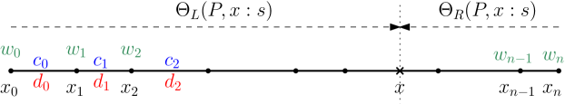
Figure 1: Example of the basic problem. Point $v_{i}$ is situated at location $x_{i}$. Edge $e_{i}=(x_{i},x_{i+1})$. $c_{i}$ is the capacity of $e_{i}.$ $d_{i}=x_{i+1}-x_{i}$ is the length of $e_{i}.$ $w_{i}$ is the initial amount of (flow) items located on $v_{i}$. $\Theta_{L}(P,x:s)$ is the time required to evacuate all items to the left of point $x$ to $x$. $\Theta_{R}(P,x:s)$ is the time required to evacuate all items to the right of point $x$ to $x$.

See Figure 1. The formal input to the Dynamic Confluent Flow on a Path problem is a path $P=(V,E)$ with $V=\{v_{0},v_{1},\ldots,v_{n}\}$ and $E=\{e_{0},e_{1},\ldots,e_{n-1}\}$ where $e_{i}=(v_{i},v_{i+1})$.

• Each edge $e_{i}$ has associated length $d_{i}=d(v_{i},v_{i+1}),$ which is the time required to travel between $v_{i}$ and $v_{i+1}.$
  $P$ is embedded on the line by placing vertex $v_{i}$ at location $x_{i}$ where $x_{0}=0$ and, $\forall i\geq 0$ $x_{i}=x_{i-1}+d_{i}=\sum_{j=0}^{i}d_{j}.$

• $x\in P$ will denote any point, not necessarily a vertex, on the segment $[0,x_{n}]$.

• Each edge $e_{i}$ also has an associated capacity $c_{i}=c(v_{i},v_{i+1})$, denoting the amount of flow that can enter $e_{i}$ in unit time.

• Scenario $s=(w_{0}(s),w_{1}(s),..,w_{n}(s))$. $w_{i}(s)$ denotes the amount of flow initially starting at vertex $v_{i}$ in scenario $s.$ This flow needs to travel to a sink, $x\in P,$ where it will be evacuated.

• For $i\leq j$, set $W_{i,j}(s)=\sum_{t=i}^{j}w_{t}(s)$.

The basic problem is to find the location of the sink $x\in P$ that minimizes the total evacuation time of all flow to $x$. If the capacities are unbounded, this reduces to the standard $1$-center problem. If capacities are bounded, congestion can arise when too much flow wants to enter an edge. This can occur in many different ways. As an example, if flow is moving from left to right and $c_{i-1}>c_{i}$, then flow enters $v_{i}$ from $e_{i-1}$ faster than it can leave $v_{i}$ to continue onto $e_{i}.$ The congestion is caused by excess flow waiting at $v_{i}$ until it can enter $v_{i}.$

Given a path $P=(V,E)$, lengths $d_{i}$, capacities $c_{i}$ and scenario $s$, the time needed to evacuate all the flow from the left of $x$, i.e., in $[0,x),$ to $x$ is denoted by $\Theta_{L}(P,x:s).$ The time needed to evacuate all the flow from the right of $x$, i.e., in $(x,x_{n}],$ to $x$ is denoted by $\Theta_{R}(P,x:s).$ The time needed to evacuate all of the flow to $x$ is the maximum of the left and right evacuation times:

$$\Theta(P,x:s)=\max\left\{\Theta_{L}(P,x:s),\Theta_{R}(P,x:s)\right\}.$$ (1)

The formulae for the left and right evacuation times require a further definition:

Definition 1 (Minimum capacity on a path).

Let $x\leq x^{\prime}$ with $x,x^{\prime}\in P$. Set

$$c(x,x^{\prime})=\min\{c_{t}\,:\,i\leq t<j\}\quad\mbox{where}\quad i=\max\{i^{\prime}\,:\,x_{i^{\prime}}\leq x\}\quad\mbox{and}\quad j=\min\{j^{\prime}\,:\,x_{j^{\prime}}\geq x^{\prime}\}.$$

Note: $c(x,x^{\prime})$ is the minimum-capacity of edges on the path connecting $x$ and $x^{\prime}.$

The formulae for $\Theta_{L}(P,x:s)$, and $\Theta_{R}(P,x:s)$ are

Lemma 2.

[3]

$$\Theta_{L}(P,x:s)=\max_{i:x_{i}<x}g_{i}(x:s)\quad\mbox{where}\quad g_{i}(x:s)=\begin{cases}d(x_{i},x)+\frac{W_{0,i}(s)}{c(x_{i},x)},&\mbox{\rm if $W_{0,i}(s)>0$},\\ 0,&\mbox{\rm if $W_{0,i}(s)=0$}.\end{cases}$$ (2)

$$\Theta_{R}(P,x:s)=\max_{i:x_{i}>x}h_{i}(x:s)\quad\mbox{where}\quad h_{i}(x:s)=\begin{cases}d(x,x_{i})+\frac{W_{i,n}(s)}{c(x,x_{i})},&\mbox{\rm if $W_{i,n}(s)>0$},\\ 0,&\mbox{\rm if $W_{i,n}(s)=0$}.\end{cases}$$ (3)

For later use, we rewrite this for the different cases of $x$ being a vertex and $x$ on an edge:

Corollary 3.

1. If $x=x_{j}$ for some $j$, then

   $$\Theta_{L}(P,x:s)=\max_{i<j}g_{i}(x_{j}:s)\quad\mbox{and}\quad\Theta_{R}(P,x:s)=\max_{i>j}h_{i}(x_{j}:s).$$

2. If $x\in(x_{j},x_{j+1})$ for some $j$,

   $$\begin{array}[]{ccccccc}\Theta_{L}(P,x:s)&=&\max\limits_{i\leq j}g_{i}(x_{j+1}:s)-(x_{j+1}-x)&\quad\mbox{and}&\Theta_{R}(P,x:s)&=&\max\limits_{i\geq j+1}h_{i}(x_{j},s)-(x-x_{j})\\[14.45377pt] &=&\Theta_{L}(P,x_{j+1}:s)-(x_{j+1}-x)&&&=&\Theta_{R}(P,x_{j}:s)-(x-x_{j}).\\ \end{array}$$

We also need the following observations

Corollary 4.

Assume $W_{0,n}>0.$

• Let $t=\min\{i\,:\,W_{0,i}>0\}.$ Then $\Theta_{L}(P,x:s)=0$ for $x\leq x_{t}$ and $\Theta_{L}(P,x:s)$ is a monotonically increasing function of $x$ for $x\geq x_{t}.$

• Let $t^{\prime}=\max\{i\,:\,W_{i,n}>0\}.$ Then $\Theta_{R}(P,x:s)=0$ for $x\geq x_{t^{\prime}}$ and $\Theta_{R}(P,x:s)$ is a monotonically decreasing function of $x$ for $x\leq x_{t^{\prime}}.$

• $\Theta_{L}(P,x:s)$ and $\Theta_{R}(P,x:s)$ are piecewise linear and continuous everywhere except, possibly, at the vertices $x_{j}.$

• $\Theta_{L}(P,x:s)$ is left continuous at $x_{j}$ and $\Theta_{R}(P,x:s)$ is right continuous at $x_{j}$, i.e.,

  $$\lim_{x\uparrow x_{j}}\Theta_{L}(P,x:s)=\Theta_{L}(P,x_{j}:s)\quad\mbox{and}\quad\lim_{x\downarrow x_{j}}\Theta_{R}(P,x:s)=\Theta_{R}(P,x_{j}:s),$$

  but can have jumps at $x_{j}$ in the other directions.

Definition 2.

The minimum time to evacuate for a given scenario over possible locations of sinks $x$ is denoted by

$$\Theta_{OPT}(P:s)=\min_{x\in P}\left\{\Theta(P,x:s)\right\}.$$

The analysis will need the following basic concepts and observations:

Definition 3.

[Critical vertex] The left and right critical vertices of $x$ under scenario $s$ are

$${\mathrm{LCV}}(x:s) = \operatorname*{arg\,max}_{i:x_{i}<x}g_{i}(x:s),$$

$${\mathrm{RCV}}(x:s) = \operatorname*{arg\,max}_{i:x_{i}>x}h_{i}(x:s).$$

${\mathrm{LCV}}(x:s)$, (resp. ${\mathrm{RCV}}(x:s)$) is the vertex at which the maximum value that defines the left (resp. right) evacuation cost is achieved. In the case of ties in achieving the maximum, $\operatorname*{arg\,max}$ will choose ${\mathrm{LCV}}(x:s)$ (resp. ${\mathrm{RCV}}(x:s)$) to be the maximizing index $i$ closest to $x.$

From Corollary 4, $\Theta_{L}(P,x:s)$ and $\Theta_{R}(P,x:s)$ are, respectively, monotonically increasing and decreasing nonnegative functions in $[x_{0},x_{n}]$ (except, respectively, for an interval at their start and finish where they might be identically zero). Thus, from Equation 1, $\Theta(P,x:s)$ first monotonically decreases in $x$, reaches a minimum and then monotonically increases in $x.$

Definition 4 (Unimodality).

Let $f(x)$ be a function defined over interval $I=[\ell,r]\subseteq\Re$. $f(x)$ is Unimodal over interval $I$, if  $\exists x^{*}\in I$ such that $f(x)$ is monotonically decreasing in $[\ell,x^{*})$ and monotonically increasing in $(x^{*},r]$. $x^{*}$ is called the mode of $f$.

The discussion preceding the definition and the fact that $\Theta_{L}(P,x:s)$ and $\Theta_{R}(P,x:s)$ are continuous everywhere except, possibly, at the points $x_{i}$, implies the following:

Observation 1.

$\Theta(P,x:s)$ is a unimodal function in $x$ over $P$. Furthermore, it is continuous everywhere except, possibly, at the points $x_{i}.$

Finally, we define

Definition 5 (Optimal Sink).

The Optimal Sink for scenario $s$ is $x_{{\mathrm{O}PT}}(s)\in[x_{0},x_{n}]$ such that

$$\Theta(P,x_{{\mathrm{O}PT}}(s):s)=\Theta_{{\mathrm{O}PT}}(P:s).$$

This optimal sink is unique because $\Theta(P,x:s)$ is a unimodal function of $x.$

By standard binary searching techniques,

Observation 2.

Let $I=[\ell,r]\subseteq[x_{0},x_{n}]$, $f(x)$ a unimodal function over $I$ and $x^{*}$ the mode of $f(x)$ in $U.$ The evaluation of $f(x_{i})$ for some $x_{i}\in I$ will be denoted as a “query”.

Then the unique index $i$ such that $x^{*}\in[x_{i},x_{i+1})$ or the fact that $x^{*}=x_{n}$ can be found using $O(\log n)$ queries.

For later use, the following will also be needed.

Lemma 5.

Let $\cal I$ be some index set (finite or infinite) and $\{f_{z}(x):z\in{\cal I}\}$ be a set of functions, all unimodal in an interval $I$. Then, if

$$f_{\max}(x)=\max_{z\in Z}f_{z}(x)$$

exists, it is also a unimodal function in $I.$

Proof.

First suppose that $f$ and $g$ are both unimodal functions with $x^{*}_{f}$, $x^{*}_{g}$ being, respectively, the unique minimum locations of of $f$ and $g$. Set $h=\max(f(x),g(x)).$

Without loss of generality assume $x^{*}_{f}\leq x^{*}_{g}$. Then $h(x)$ is monotonically decreasing for $x<x^{*}_{f}$ and monotonically increasing for $x\geq x^{*}_{g}.$ Now consider $x\in I^{\prime}=[x^{*}_{f},x^{*}_{g}]$: $f(x)$ is monotonically increasing in $I^{\prime}$, while $g(x)$ is monotonically decreasing in $I^{\prime}$.

If $f(x^{*}_{f})\geq g(x^{*}_{f})$ then

$$\forall x\in I^{\prime},\quad f(x)\geq f(x^{*}_{f})\geq g(x^{*}_{f})\geq g(x)$$

so $h$ is unimodal with mode $x^{*}_{f}$. If $f(x^{*}_{g})\leq g(x^{*}_{g})$ then

$$\forall x\in I^{\prime},\quad f(x)\leq f(x^{*}_{g})\leq g(x^{*}_{g})\leq g(x)$$

so $h$ is unimodal with mode $x^{*}_{g}$.

Otherwise $f(x^{*}_{f})<g(x^{*}_{f})$ and $f(x^{*}_{g})>g(x^{*}_{g})$ so $\bar{x}=\sup\{x\in I^{\prime}\,:\,f(x)\leq g(x)\}$ exists and

$$\forall x\in[x^{*}_{f},\bar{x}],\,f(x)\leq g(x)\mbox{ so }h(x)=g(x)\quad\mbox{and}\quad\forall x\in(\bar{x},x^{*}_{g}],\,f(x)>g(x)\mbox{ so }h(x)=f(x)$$

and $h$ is unimodal with mode $\bar{x}$.

Repeating this process yields that for any three unimodal functions $f(x),g(x),u(x)$, the function $\max\left(f(x),g(x),u(x)\right)$ is also unimodal.

Now suppose that $f_{\max}(x)$ is not unimodal. Then there exist 3 points $x_{1}<x_{2}<x_{3}$ such that $f_{\max}(x_{1})<f_{\max}(x_{2})>f_{\max}(x_{3})$. Then there exists three functions $f_{1},f_{2},f_{3}$ in the set $\{f_{z}\,:\,z\in Z\}$ satisfying $f_{\max}(x_{i})=f(x_{i})$ for $i=1,2,3.$ But this contradicts the fact that $\max\left(f_{1}(x),f_{2}(x),f_{3}(x)\right)$ is also unimodal. ∎

2.2 Regret

One method for capturing uncertainty in the input is the min-max regret viewpoint. In this, the vertex weights are not fully specified in advance. Instead, a range of weights $[w_{i}^{-},w_{i}^{+}]$ in which $w_{i}(s)$ must lie is specified. A specific assignment of weights to the vertices is a legal scenario. The set of all possible legal scenarios is the Cartesian product of all possible ranges for the weights.

$$\mathcal{S}=\prod_{i=0}^{n}[w_{i}^{-},w_{i}^{+}]$$

Definition 6.

Let $i,j$ satisfy $0\leq i\leq j\leq n$ and $\alpha,\beta\geq 0$.

• Let $s$ be a scenario. Set $s_{-i,-j}(\alpha,\beta)$ and $s_{-i}(\alpha)$ to be the unique scenarios satisfying

  $$w_{t}\left(s_{-i,-j}(\alpha,\beta)\right)=\begin{cases}w_{t}(s)&\mbox{if $t\not\in\{i,j\}$},\\ \alpha&\mbox{if \ $t=i$},\\ \beta&\mbox{if \ $t=j$}.\\ \end{cases},\hskip 14.45377ptw_{t}\left(s_{-i}(\alpha)\right)=\begin{cases}w_{t}(s)&\mbox{if $t\not=i$},\\ \alpha&\mbox{if \ $t=i$}.\end{cases}$$

  Note that in some proofs, we will have $i=j.$ In those cases, it will be required that $\alpha=\beta$ so that $s_{-i,-j}(\alpha,\beta)=s_{-i}(\alpha)$.

• Set $s^{\prime}_{i,j}$ to be the scenario satisfying

  $$w_{t}\left(s^{\prime}_{i,j}\right)=\begin{cases}w_{t}^{-}&\mbox{if \ $t<i$ or $j<t$},\\ w_{t}^{+}&\mbox{if \ $i<t<j$},\\ 0&\mbox{if \ $t\in\{i,j\}$}.\\ \end{cases}$$

• See Figure 2. Define $s_{i,j}(\alpha,\beta)=s_{-i,-j}(\alpha,\beta)$ where $s=s^{\prime}_{i,j}.$

• For any fixed $i,j,$ the corresponding set of two-varying scenarios is

  $$S_{i,j}=\left\{s_{i,j}(\alpha,\beta)\,:\,\alpha\in\left[w_{i}^{-},w^{+}_{i}\right]\mbox{ and }\beta\in\left[w_{j}^{-},w^{+}_{j}\right]\right\}.$$

Figure 2: Illustration of two varying scenario $s=s_{i,j}(\alpha,\beta).$ All vertices $v_{t}$ with $t<i$ or $t>j$ have $w_{t}(s)=w_{t}^{-}$ and all vertices $t$ with $i<t<j$ have $w_{t}(s)=w^{+}_{t}.$ Finally $w_{i}(s)=\alpha$ and $w_{j}(s)=\beta$.

In all the definitions that follow, input path $P=(V,E)$, is considered as fixed and given.

Definition 7 (Regret for $x$ under scenario $s$).

The regret for a location $x$ under scenario $s$ is

$$R(P,x:s)=\Theta(P,x:s)-\Theta_{OPT}(P:s).$$ (4)

This is the difference between evacuation time to $x$ and the optimal evacuation time.

Definition 8 (Max-regret for $x$).

The Max-regret over all possible legal scenarios for $x$ is:

$$R_{\max}(P,x)=\max_{s\in\mathcal{S}}\left\{R(P,x:s)\right\}$$ (5)

Definition 9 (Worst-case scenario).

Scenario $s\in\mathcal{S}$ is a worst-case scenario for $x$ if

$$R_{\max}(P,x)=R(P,x:s)$$ (6)

Definition 10 (Minmax regret).

The Min-Max Regret value is the minimum possible Max-regret over all possible locations $x$:

$$R_{OPT}(P)=\min_{x\in P}\left\{R_{\max}(P,x)\right\}$$ (7)

The goal is to find $x\in P$ such that $R_{OPT}(P)=R_{\max}(P,x).$

2.3 Technical Observations for later use

Lemma 6.

Let $I=[x_{0},x_{n}]$. Then

1. For every $s\in\mathcal{S}$, $R(P,x:s)$ is a unimodal function of $x$ over $I$.

2. $R_{\max}(P,x)$ is a unimodal function of $x$ over $I$.

Furthermore $R(P,x:s)$ and $R_{\max}(P,x)$ are continuous everywhere except, possibly, at the $x_{i}.$

Proof.

(1) follows from Observation 1 and the fact that subtracting a constant from a unimodal function leaves a unimodal function.

(2) follows from (1) and Lemma 5.

The continuity of $R(P,x:s)$ follows directly from the continuity of $\Theta(P,x:s)$; the continuity of $R_{\max}(P,x)$ follows from the continuity of $R(P,x:s)$. ∎

The following technical lemma will be needed later for the correctness of the algorithm.

Lemma 7.

Let $\ell<r$ and $f_{\ell}$, $f_{r}$, $g_{\ell}$ and $g_{r}$ be constants satisfying

$$f_{\ell}\leq f_{r}-(r-\ell),\quad g_{r}\leq g_{\ell}-(r-\ell).$$ (8)

For all $x\in[\ell,r]$, define

$$f(x)=\begin{cases}f_{\ell}&\mbox{if $x=\ell$},\\ f_{r}-(r-x)&\mbox{if $x\in(\ell,r)$, }\\ f_{r}&\mbox{if $x=r$},\\ \end{cases}\quad\mbox{and}\quad g(x)=\begin{cases}g_{\ell}&\mbox{if $x=\ell$},\\ g_{\ell}-(x-\ell)&\mbox{if $x\in(\ell,r)$, }\\ g_{r}&\mbox{if $x=r$}\end{cases}$$

and

$$\bar{f}(x)=\begin{cases}f_{r}-(r-\ell)&\mbox{if $x=\ell$},\\ f(x)&\mbox{if $x\in(\ell,r]$, }\\ \end{cases}\quad\mbox{and}\quad\bar{g}(x)=\begin{cases}g(x)&\mbox{if $x\in[\ell,r)$},\\ g_{r}&\mbox{if $x=r$.}\end{cases}$$

Note that $f(x)$ (resp. $g(x)$) is continuous everywhere except possiby at the endpoint $x=\ell$ (resp. $x=r$) while $\bar{f}(x)$ (reps. $\bar{g}(x)$)) is continuous everywhere.

Finally for all $x\in[\ell,r]$ define

$$h(x)=\max\left(f(x),g(x)\right)\quad\mbox{and}\quad\bar{h}(x)=\max\left(\bar{f}(x),\bar{g}(x)\right)$$

Then $\min_{x\in[\ell,r]}h(x)$ exists and

$$\min_{x\in[\ell,r]}h(x)=X\quad\mbox{where}\quad X=\min\left(h(\ell),\,h(r),\,\min_{x\in[\ell,r]}\bar{h}(x)\right).$$

Proof.

Technically, because $h(x)$ might not be continuous at $\ell,r,$ only the existence of $\inf_{x\in[\ell,r]}h(x)$ is known. Proving the lemma requires also proving that $\min_{x\in[\ell,r]}h(x)$ also exists.

From the definitions,

$$h(\ell)=\max\left(f(\ell),g(\ell)\right)\leq\max\left(\bar{f}(\ell),\bar{g}(\ell)\right)=\bar{h}(\ell)$$

and

$$h(r)=\max\left(f(r),g(r)\right)\leq\max\left(\bar{f}(r),\bar{g}(r)\right)=\bar{h}(r).$$

Since $\bar{h}$ is a continuous bounded function in $[\ell,r]$, $Y=\min_{x\in[\ell,r]}\bar{h}(x)$ exists, so $X$ also exists.

Now let $x^{*}\in[\ell,r]$ be such that $Y=\bar{h}(x^{*})$. If $x^{*}\in(\ell,r)$, then since $h(x)=\bar{h}(x)$ for all $x\in(\ell,r)$,

$$\inf_{x\in[\ell,r]}h(x)=\min\left(h(\ell),\,h(r),\,h(x^{*})\right)=X.$$

If $x^{*}\not\in(\ell,r)$ then $x^{*}\in\{\ell,r\}$ so $Y=\min\left(\bar{h}(\ell),\bar{h}(r)\right)$. Since $h(\ell)\leq\bar{h}(\ell)$ and $h(r)\leq\bar{h}(r)$,

$$\inf_{x\in[\ell,r]}h(x)=\min\left(h(\ell),\,h(r),\,\bar{h}(\ell),\,\bar{h}(r)\right)=\min\left(h(\ell),\,h(r)\right)=X.$$

In both the cases, we have shown that $\inf_{x\in[\ell,r]}h(x)=X$ and that the infimum is achieved at some value $h(x)$, $x\in[\ell,r]$ so $\min_{x\in[\ell,r]}h(x)=\inf_{x\in[\ell,r]}h(x)=X.$

∎

The later proof of Lemma 21 will also require the following simple corollary:

Corollary 8.

Fix $k$ and some scenario $s\in{\mathcal{S}}.$ Then

$$\min_{y\in[x_{k},x_{k+1}]}\Theta(P,y:s)=\small\min\small\left(\Theta(P,x_{k}:s),\,\Theta(P,x_{k+1}:s),\,Y\right).$$

where

$$Y=\min_{y\in[x_{k},x_{k+1}]}\max\bigl{\{}\Theta_{L}(P,x_{k+1}:s)-(x_{k+1}-x),\Theta_{R}(P,x_{k}:s)-(x-x_{k})\bigr{\}}$$

Proof.

Set $\ell=x_{k}$, $r=x_{k+1}$ and

$$\begin{array}[]{ccccccc}f_{\ell}&=&\Theta_{L}(P,x_{k}:s),&&f_{r}&=&\Theta_{L}(P,x_{k+1}:s),\\ g_{\ell}&=&\Theta_{R}(P,x_{k}:s),&&g_{r}&=&\Theta_{R}(P,x_{k+1}:s).\end{array}$$

From Corollaries 3 and 4, Equation 8 is satisfied. Also from Corollary 3, for $x\in(x_{k},x_{k+1})$

$$\begin{array}[]{cllcc}f(x)&=&\Theta_{L}(P,x_{k+1}:s)-(x_{k+1}-x)&=&\Theta_{L}(P,x:s),\\ g(x)&=&\Theta_{R}(P,x_{k}:s)-(x-x_{k})&=&\Theta_{R}(P,x:s).\end{array}$$

The proof of the Corollary then follows directly from Lemma 7. ∎

3 Reduction to scenarios with two varying weights

As the scenario space $\mathcal{S}$ is infinite, it is impossible to calculate $R_{\max}(P,x)$ directly from Equation 5. To sidestep this, the standard approach, e.g., [14, 24, 18, 7], for the uniform capacity case has been to first reduce the scenario space to a finite set of possible worst-case scenarios.

As the first step in this direction for general capacities, we start with a lemma describing the effect of changing weights of a single vertex in a scenario.

Definition 11.

Let $s\in\mathcal{S}.$ $s^{\prime}\in\mathcal{S}$ is obtained from $s$ by the operation $\texttt{SHIFT}(i,j,\delta)$ by setting

$$w_{t}(s^{\prime})=\left\{\begin{array}[]{ll}w_{i}(s)-\delta&\mbox{if $t=i$},\\ w_{j}(s)+\delta&\mbox{if $t=j$},\\ w_{t}(s)&\mbox{if $t\not=i,j$}.\\ \end{array}\right.$$

Note that $\texttt{SHIFT}(i,j,\delta)$ is a valid operation only if $w_{i}(s)\geq w_{i}^{-}+\delta$ and $w_{j}\leq w_{j}^{+}-\delta$.

Lemma 9.

Let $s^{\prime}\in\mathcal{S}$ be obtained from $s\in\mathcal{S}$ by applying a valid $\texttt{SHIFT}(i,j,\delta)$ operation.

• If $i<j$ and $x_{j}\leq x$, then $\Theta(P,x:s^{\prime})\leq\Theta(P,x:s).$

• If $j<i$ and $x\leq x_{i}$, then $\Theta(P,x:s^{\prime})\leq\Theta(P,x:s).$

Proof.

We prove (a). The proof of (b) is symmetric.

Consider the formula in Lemma 2. For every $k$, $W_{0,k}(s^{\prime})\leq W_{0,k}(s)$. Thus, $\Theta_{L}(P,x:s^{\prime})\leq\Theta_{L}(P,x:s)$. Furthermore, for every $k$ satisfying $x\leq x_{k}$, $W_{k,n}(s^{\prime})=W_{k,n}(s)$. Thus $\Theta_{R}(P,x:s^{\prime})=\Theta_{R}(P,x:s)$. The proof of the Lemma follows immediately. ∎

Given a set of scenarios ${\cal S}^{\prime}\subseteq{\cal S}$, vertex $x_{i}$ is varying in ${\cal S}^{\prime}$ if $w_{i}(s)$ not constant for all $s\in{\cal S}^{\prime}.$ In the full set $\cal S$ of all possible scenarios, all the vertices might be varying. The important observation will be that, when considering sets of worst-case scenarios, it suffices to consider subsets in which only two vertices are varying and the rest have fixed weights, i.e., the sets $S_{i,j}$.

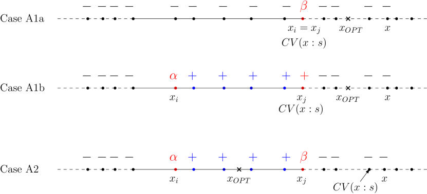
Figure 3: Illustration of the three possible worse-case scenarios that can occur in Case A in Theorem 10. In all three cases, $\Theta(P,x)$ is the time for evacuation from the left. $CV(x:s)$ is the index of the critical vertex in the evacuation from the left. $x_{{\mathrm{O}PT}}$ is the location of the optimal sink (that minimizes evacuation time). In case A1a, $i=j$ while in case A1b, $i<j$ but $w_{j}(s)=w^{+}_{j}$. In both A1 scenarios, $x_{j}$ is the critical vertex and $x_{j}\leq x_{{\mathrm{O}PT}}\leq x$. In case 2, the critical vertex can be anywhere between $x_{j}$ and $x$ and $x_{i}\leq x_{{\mathrm{O}PT}}\leq x_{j}.$

Theorem 10.

Let $x\in P.$ There exists a worst case scenario $s$ for $x$, such that $s\in S_{i,j}$ for some $i<j$ and at least one of the following conditions is true. See Figure 3.

• $\Theta(P,x:s)=\Theta_{L}(P,x:s)$ and

  1. ${\mathrm{LCV}}(x:s)=j$ where $x_{j}\leq x_{{\mathrm{O}PT}}(s)\leq x$, $x_{j}<x$ and

     • Either $i=j$ (so $s\in S_{j,j}$)

     • or $i<j$ and $w_{j}(s)=w_{j}^{+}$

  2. or ${\mathrm{LCV}}(x:s)\geq j$ and $x_{i}\leq x_{{\mathrm{O}PT}}(s)\leq x_{j}\leq x$

• $\Theta(P,x:s)=\Theta_{R}(P,x:s)$ and

  1. ${\mathrm{RCV}}(x:s)=i$ where $x\leq x_{{\mathrm{O}PT}}(s)\leq x_{i}$, $x<x_{i}$ and

     • Either $i=j$ (so $s\in S_{i,i}$)

     • or $i<j$ and $w_{i}(s)=w_{i}^{+}$

  2. or ${\mathrm{RCV}}(x:s)\leq i$ and $x\leq x_{i}\leq x_{{\mathrm{O}PT}}(s)\leq x_{j}$

Proof.

Let $s$ be a worst-case scenario for $x$. We apply a series of transformations to $s$, converting it to $s^{*}$, maintaining the property that at each step, the currently constructed scenario remains a worst-case scenario for $x$. The final constructed scenario $s^{*}$ will satisfy the conditions of the theorem.

Without loss of generality, assume that $\Theta(P,x:s)=\Theta_{L}(P,x:s)\geq\Theta_{R}(P,x:s)$. We prove that a worst-case $s^{\prime}$ satisfying (A) exists. The proof for (B) when $\Theta(P,x:s)=\Theta_{R}(P,x:s)$ will be totally symmetric.

First note that if $x<y$, then by the monotonicity of both $\Theta_{L}(P,y:s)$ and $\Theta_{R}(P,y:s)$ in $y$,

$$\Theta_{L}(P,x:s)<\Theta_{L}(P,y:s)\quad\mbox{and}\quad\Theta_{R}(P,x:s)>\Theta_{R}(P,y:s).$$

Thus

$$\Theta(P,y:s)=\max\{\Theta_{L}(P,y:s),\Theta_{R}(P,y:s)\}>\Theta_{L}(P,x:s)=\Theta(P,x:s)$$

and $y\not=x_{{\mathrm{O}PT}}(s).$ Thus, $x_{{\mathrm{O}PT}}(s)\leq x.$

For notational simplicity, now set $k={\mathrm{LCV}}(x:s)$ and $y=x_{{\mathrm{O}PT}}(s)$. By the argument above, $y\leq x$. Also, by the definition of ${\mathrm{LCV}}(x:s)$, $x_{k}<x.$

Next, change the weights of all vertices $i>k$ to $w_{i}^{-}$. Denote the resulting scenario as $s^{\prime}$. As no weights are increased, $\Theta_{R}(P,x:s^{\prime})\leq\Theta_{R}(P,x:s)$ and $\Theta_{OPT}(P:s^{\prime})\leq\Theta_{OPT}(P:s)$. Note that the weights in $[v_{0},v_{k}]$ are unchanged and weights to the right of $v_{k}$ can only decrease. From the definition of $k={\mathrm{LCV}}(x:s)$,

$$\Theta_{L}(P,x:s^{\prime})=g_{k}(x:s^{\prime})=g_{k}(x:s)=\Theta_{L}(P,x:s)\geq\Theta_{R}(P,x:s)\geq\Theta_{R}(P,x:s^{\prime}).$$

Thus,

$$\Theta(P,x:s^{\prime}) = \max\left\{\Theta_{L}(P,x:s^{\prime}),\Theta_{R}(P,x:s^{\prime})\right\}$$

$$= \Theta_{L}(P,x:s)$$

$$= \Theta(P,x:s).$$

This yields

$$\Theta(P,x:s^{\prime})-\Theta_{OPT}(P:s^{\prime})\geq\Theta(P,x:s)-\Theta_{OPT}(P:s)$$

Thus, $s^{\prime}$ is also a worst case scenario for $x$. Henceforth, we may assume that $w_{i}(s)=w_{i}^{-}$ for $i>k$.

Case-1: $y=x_{{\mathrm{O}PT}}(s)\geq x_{k}$

As long as there exists a $i,j,\delta$ that permits a valid shift operation, apply $\texttt{SHIFT}(i,j,\delta),i<j\leq k$. Utilize the rule of always choosing the smallest $i$ that currently has more than $w_{i}^{-}$ flow and largest $j$ that currently has less than $w_{j}^{+}$ flow. When applying the shift to $i,j$, choose the largest possible $\delta$ that maintains validity. Then, either $w_{i}$ is set to $w^{-}_{i}$ or $w_{j}$ is set to $w^{+}_{j}$. This process must therefore conclude after at most $k$ shift operations. Denote the final resulting scenario by $s^{\prime}$. This construction is pushing units of flow to the right, towards $k$. Thus by construction, it must end in one of the following two cases

• If $w_{k}(s^{\prime})<w_{k}^{+}$, then $\forall t\leq k,$ $w_{t}(s^{\prime})=w^{-}_{t}$, so $s^{\prime}\in S_{k,k}.$

• If $w_{k}(s^{\prime})=w_{k}^{+}$, let $i<k$ be the largest index such that $w_{i}(s^{\prime})>w_{i}^{-}.$ Then $\forall t<i$, $w_{t}(s^{\prime})=w_{t}^{-}$ and $\forall i<t\leq k$, $w_{t}(s^{\prime})=w^{+}_{t}$ so $s^{\prime}\in S_{i,k}$,

The constructed scenarios are then of type A1a or A1b after setting $j=k$. Note that this implies $x_{j}=x_{k}<x.$

To prove that this set of operations indeed preserves the worst-case property, first note that, by construction, $W_{0,t}(s^{\prime})=W_{0,t}(s)$ for all $t\geq j.$ In particular, this implies that $W_{0,j}(s^{\prime})=W_{0,j}(s)$. Since $j=k={\mathrm{LCV}}(x:s),$ from the definition of $g_{j}(x,s),$

$$\Theta(P,x:s^{\prime})\geq g_{j}(x:s^{\prime})=g_{j}(x,s)=\Theta(P,x:s).$$ (9)

Set $y^{\prime}=x_{{\mathrm{O}PT}}(s^{\prime})$ and $j^{\prime}={\mathrm{LCV}}(x:s^{\prime})$. (A-priori, it is possible that $j^{\prime}\not=j$ or $y\not=y^{\prime}.$)

From Lemma 9(a) and the assumption $y\geq x_{k}=x_{j},$

$$\Theta(P,y^{\prime}:s^{\prime})=\Theta_{OPT}(P:s^{\prime})\leq\Theta(P,y:s^{\prime})\leq\Theta(P,y:s)=\Theta_{OPT}(P:s).$$ (10)

Thus, from Equations 9 and 10,

$$\Theta(P,x:s^{\prime})-\Theta_{OPT}(P:s^{\prime}) \geq \Theta(P,x:s^{\prime})-\Theta_{OPT}(P:s)$$

$$\geq \Theta(P,x:s)-\Theta_{OPT}(P:s)=R_{\max}(P,x)$$

so $s^{\prime}$ is also a worse-case scenario for $x$.

To complete the proof of Case 1 for $s^{\prime}$, it suffices to show that $j=j^{\prime}$ and $y=y^{\prime}$. Note that $\Theta(P,x:s^{\prime})\geq\Theta(P,x,s)$ and $\Theta_{OPT}(P:s^{\prime})\leq\Theta_{OPT}(P:s)$. If either $\Theta(P,x:s^{\prime})>\Theta(P,x:s),$ or $\Theta_{OPT}(P:s^{\prime})<\Theta_{OPT}(P:s)$ then

$$\Theta(P,x:s^{\prime})-\Theta_{OPT}(P:s^{\prime})>R_{\max}(P,x),$$

contradicting the definition of $R_{\max}(P,x)$. Thus $\Theta_{OPT}(P:s^{\prime})=\Theta_{OPT}(P:s)$ and $\Theta(P,x:s^{\prime})=\Theta(P,x:s).$ Plugging the first equality into Equation 10 immediately yields

$$\Theta(P,y^{\prime}:s^{\prime})=\Theta_{OPT}(P:s^{\prime})=\Theta(P,y:s^{\prime})=\Theta_{OPT}(P:s)$$ (11)

so

$$y^{\prime}=y.$$

Furthermore, the second equality and the fact that $W_{0,t}(s^{\prime})=W_{0,t}(s)$ for all $t\geq j$ immediately implies that

$$j^{\prime}={\mathrm{LCV}}(x:s^{\prime})={\mathrm{LCV}}(x:s)=j.$$

Case-2: $y=x_{{\mathrm{O}PT}}(s)<x_{k}$

Let $u<k$ be the largest index such that $x_{u}\leq y<x_{k}$.

First apply $\texttt{SHIFT}(i,j,\delta),i<j\leq u$ if there exists a $i,j,\delta$ that permits a valid operation, using the same rule as in Case-1. By the same argument as in Case 1, these shifts can be shown to terminate after a finite number of steps. Let $s^{\prime}$ be the resulting scenario. Note that after completing these shifts, one of the following two situations must occur:

• Either $w_{u}(s^{\prime})<w^{+}_{u}$, and thus $w_{t}(s^{\prime})=w^{-}_{t}$ for all $t<u$.

• or $w_{u}(s^{\prime})=w^{+}_{u}$ and there exists $p<u$ such that $w_{t}(s^{\prime})=w^{-}_{t}$ for all $t<p$ and $w_{t}(s^{\prime})=w^{+}_{t}$ for all $p<t\leq u.$

Next, apply $\texttt{SHIFT}(j,i,\delta),y\leq x_{i}<x_{j}\leq x_{k}$ if there exists a $i,j,\delta$ that permits a valid operation. Now use the rule of always choosing the smallest $i$ that currently has less than $w_{i}^{+}$ flow and largest $j$ that currently has more than $w_{j}^{-}$ flow. Again, always choose the largest possible $\delta$ valid for the $i,j$ pair. These operations also terminate after a finite number of steps. After the termination of this seconds set of shifts, the new resulting scenario $s^{\prime}$ satisfies

• There exists $q,$ $u\leq q\leq k$ such that $w_{t}(s^{\prime})=w^{+}_{t}$ for all $u<t<q$ and $w_{t}(s^{\prime})=w^{-}_{t}$ for all $q<t\leq k$

Combining this with the fact that,

• $\forall t\geq k,$ $w_{t}(s^{\prime})=w_{t}(s)=w^{-}_{t}$

yields that $s^{\prime}\in S_{p,q}$ with $x_{p}\leq x_{u}\leq y\leq x_{q}\leq x_{k}.$

Set $y^{\prime}=x_{{\mathrm{O}PT}}(s^{\prime})$ and $k^{\prime}={\mathrm{LCV}}(x:s^{\prime})$.

The proof that $s^{\prime}$ is also a worst-case scenario for $x$ is similar to that in Case 1.

By construction, $W_{0,t}(s^{\prime})=W_{0,t}(s)$ for all $t\geq k.$ In particular, this implies that $W_{0,k}(s^{\prime})=W_{0,k}(s)$. Since $k={\mathrm{LCV}}(x:s)$,

$$\Theta(P,x:s^{\prime})\geq g_{k}(x:s^{\prime})=g_{k}(x,s)=\Theta(P,x:s).$$

Both types of shifts (to the right and to the left) applied above satisfy the conditions in  Lemma 9((a) and (b)) with respect to $y=x_{OPT}$. Applying  Lemma 9 and applying the same argument following  Equation 9 yields that  Equation 11 is correct for this case as well.

The exact same arguments as in Case-1 then show that $s^{\prime}$ is a worst-case scenario for $x$, $y^{\prime}=y$ and $k^{\prime}=k$ completing the proof of Case 2 after setting $i=p$ and $j=q$. Note that $x_{j}=x_{q}\leq x_{k}<x.$ ∎

Definition 12.

Let $i<j$. Set

$$G_{j}(x)=\max_{s\in S_{j,j}}\left\{g_{j}(x:s)-\min_{y\,:\,x_{j}\leq y\leq x_{n}}\Theta(P,y:s)\right\}\quad\mbox{and}\quad H_{i}(x)=\max_{s\in S_{i,i}}\left\{h_{i}(x:s)-\min_{y\,:\,x_{0}\leq y\leq x_{i}}\Theta(P,y:s)\right\}.$$

These correspond, respectively, to Cases A1a and B1a of Theorem 10.

Now set

$$G_{i,j}(x) = \max_{s\in S_{i,j},w_{j}(s)=w_{j}^{+}}\left\{g_{j}(x:s)-\min_{y\,:\,x_{j}\leq y\leq x_{n}}\Theta(P,y:s)\right\},$$

$$\bar{G}_{i,j}(x) = \max_{s\in S_{i,j}}\left\{\left(\max_{t\,:\,x_{j}\leq x_{t}\leq x}g_{t}(x:s)\right)-\min_{y\,:\,x_{i}\leq y\leq x_{j}}\Theta(P,y:s)\right\},$$

$$H_{i,j}(x) = \max_{s\in S_{i,j},w_{i}(s)=w_{i}^{+}}\left\{h_{i}(x:s)-\min_{y\,:\,x_{0}\leq y\leq x_{i}}\Theta(P,y:s)\right\},$$

$$\bar{H}_{i,j}(x) = \max_{s\in S_{i,j}}\left\{\left(\max_{t\,:\,x\leq x_{t}\leq x_{i}}h_{t}(x:s)\right)-\min_{y\,:\,x_{i}\leq y\leq x_{j}}\Theta(P,y:s)\right\},$$

These correspond, respectively, to Cases A1b, A2, B1b and B2 of Theorem 10.

Next, define

Definition 13.

For $x\in P$ define

$$G(x)=\max\left\{\max_{j\,:\,x_{0}\leq x_{j}<x}G_{j}(x),\,\max_{\begin{subarray}{c}(i,j)\\ {x_{0}\leq x_{i}<x_{j}<x}\end{subarray}}G_{i,j}(x),\,\max_{\begin{subarray}{c}(i,j)\\ {x_{0}\leq x_{i}<x_{j}<x}\end{subarray}}\bar{G}_{i,j}(x)\right\}$$

$$H(x)=\max\left\{\max_{i\,:\,x<x_{i}\leq x_{n}}H_{i}(x),\,\max_{\begin{subarray}{c}(i,j)\\ {x<x_{i}<x_{j}\leq x_{n}}\end{subarray}}H_{i,j}(x),\,\max_{\begin{subarray}{c}(i,j)\\ {x<x_{i}<x_{j}\leq x_{n}}\end{subarray}}\bar{H}_{i,j}(x)\right\}$$

Theorem 10 then immediately implies the main theoretical result of this paper:

Theorem 11.

$$R_{\max}(P,x)=\max\left\{G(x),\,H(x)\right\}.$$

Proof.

By construction, each of the terms comprising $G(x)$ and $H(x)$ are lower bounds on $R_{\max}(P,x).$ This is because, if $x_{t}<x$, for any scenario $s$ and any $y\in P$,

$$\Theta(P,x:s)\geq\Theta_{L}(P,x:s)\geq g_{t}(x:s)\quad\mbox{and}\quad\Theta_{OPT}(P:s)\leq\Theta(P,y:s)$$

so

$$R_{\max}(P,x)\geq R(P,x:s)=\Theta(P,x:s)-\Theta_{OPT}(P:s)\geq g_{t}(x:s)-\Theta(P,y:s).$$

Plugging into the formulas given in Definitions 12 and 13 immediately shows that $R_{\max}(P,x)\geq G(x).$ The proof that $R_{\max}(P,x)\geq H(x)$ is similar.

Theorem 10 shows that $R_{\max}(P,x)$ is achieved by one of the cases that $G(x)$ and $H(x)$ are enumerating, proving correctness. ∎

The minimization ranges in Definition 12

We note that the definitions of $G_{j}$ and $G_{i,j}$ could be modified without affecting validity. More explicitly, the range “${y\,:\,x_{j}\leq y\leq x_{n}}$” in their inner minimizations could be replaced by “${y\,:\,x_{j}\leq y\leq x}$” to more closely mirror the statement of Theorem 10. Theorem 11 would remain correct under this replacement. The longer ranges are used to simplify the statements of the later evaluation procedures. A similar replacement of “${y\,:\,x_{0}\leq y\leq x_{i}}$” with “${y\,:\,x\leq y\leq x_{i}}$” could be made in the definitions of $H_{i}$ and $H_{i,j}.$

Comparison to the uniform capacity case

It is instructive at this point to compare the result above to what is known in the uniform capacity case.

For the uniform capacity case on paths, it is known [14, 24, 18, 7] that the set of $s_{0,0}(w_{0}^{-},w_{0}^{-})$ ( i.e., all $w_{i}^{-}$s) and the scenarios $s_{0,j}(w_{0}^{+},w_{j}^{+})$ or $s_{j,n}(w_{j}^{+},w_{n}^{+})$ for some $j$ provide the worst-case scenarios for all the sinks. This implies the existence of a simple $O(n)$ sized set of worst-case scenarios, all structurally independent of the actual input values. The existence of this set is the cornerstone of the fast (best case $O(n)$ [7]) algorithms for this problem. Similar structural results hold for the worst-case scenarios for the uniform-capacity minmax regret $k$-sink on a path [3] problem and one sink on a tree problem [7].

In contrast, in the general capacities case, no such simple finite set of worst-case scenarios seem to exist. Theorem 10 reduces the search space of worst-case scenarios substantially, but not to a finite set.

We now study some properties of the functions $G(x)$ and $H(x)$ that will be useful later.

Lemma 12.

1. Let $x\in\left(x_{u},x_{u+1}\right).$ Then

   $$\quad G(x)=G(x_{u+1})-(x_{u+1}-x),\quad\mbox{and}\quad H(x)=H(x_{u})-(x-x_{u}).$$ (12)

2. Let $0\leq u<n.$ Then

   $$G(x_{u})\leq G(x_{u+1})-(x_{u+1}-x_{u}),\quad\mbox{and}\quad H(x_{u+1})\leq H(x_{u})-(x_{u+1}-x_{u}).$$

Proof.

Let $x\in(x_{u},x_{u+1})$ and $s\in S_{ij}.$ From Lemmas 2 and 3,

$$\forall t\leq u,\quad g_{t}(x:s)=g_{t}(x_{u+1}:s)-(x_{u+1}-x)\quad\mbox{and}\quad\forall i\geq u+1,\quad h_{i}(x:s)=h_{i}(x_{u}:s)-(x_{u+1}-x).$$

Directly plugging in the formulas from Definition 12 yields, for all $x\in(x_{u},x_{u+1}),$

$$G_{j}(x) =G_{j}(x_{u+1})-(x_{u+1}-x), H_{i}(x) =H_{i}(x_{u})-(x-x_{u}),$$

$$G_{i,j}(x) =G_{i,j}(x_{u+1})-(x_{u+1}-x), H_{i,j}(x) =H_{i,j}(x_{u})-(x-x_{u}),$$

$$\bar{G}_{i,j}(x) =\bar{G}_{i,j}(x_{u+1})-(x_{u+1}-x), \bar{H}_{i,j}(x) =\bar{H}_{i,j}(x_{u})-(x-x_{u}).$$

(1.) then follows from the definition of $G(x)$ and $H(x)$.

Similarly, from Lemmas 2 and 3, for every $s\in S_{i,j}$, we get

$$\forall t<u,\quad g_{t}(x_{u}:s)=g_{t}(x_{u+1}:s)-(x_{u+1}-x_{u})\quad\text{and}\quad\forall i>u+1,\quad h_{i}(x_{u+1})=h_{i}(x_{u})-(x_{u+1}-x_{u})$$

Plugging these formulas into the definitions again yields

$$G(x_{u}) = \max\left\{\max_{j\,:\,x_{0}\leq x_{j}<x_{u}}G_{j}(x_{u+1}),\,\max_{\begin{subarray}{c}(i,j)\\ {x_{0}\leq x_{i}<x_{j}<x_{u}}\end{subarray}}G_{i,j}(x_{u+1}),\,\max_{\begin{subarray}{c}(i,j)\\ {x_{0}\leq x_{i}<x_{j}<x_{u}}\end{subarray}}\bar{G}_{i,j}(x_{u+1})\right\}-(x_{u+1}-x_{u})$$

$$\leq \max\left\{\max_{j\,:\,x_{0}\leq x_{j}<x_{u+1}}G_{j}(x_{u+1}),\,\max_{\begin{subarray}{c}(i,j)\\ {x_{0}\leq x_{i}<x_{j}<x_{u+1}}\end{subarray}}G_{i,j}(x_{u+1}),\,\max_{\begin{subarray}{c}(i,j)\\ {x_{0}\leq x_{i}<x_{j}<x_{u+1}}\end{subarray}}\bar{G}_{i,j}(x_{u+1})\right\}-(x_{u+1}-x_{u})$$

$$= G(x_{u+1})-(x_{u+1}-x_{u}),$$

proving the left side of (2.). Note that the difference between the first and second lines is the extension of the ranges on which the maximum is taken.

The proof of the right side of (2.), that $H(x_{u+1})\leq H(x_{u})-(x_{u+1}-x_{u}),$ is similar. ∎

The next section uses the structural information provided by this section to derive a $O(n^{4})$ procedure for finding a worst case scenario for $x.$

4 The Algorithm

Theorems 11 and 12 permit efficient calculation of $R_{OPT}(P)$.

Lemma 13.

Let $U(n)$ be the time required to calculate $H(x_{i})$ and $G(x_{i})$ for any $x_{i}\in P.$ Then $R_{OPT}(P)$ can be calculated in $O(U(n)\log n)$ time.

Proof.

First note that, from Theorem 11,

$$R_{\max}(P,x_{i})=\max\left\{G(x_{i}),\,H(x_{i})\right\}$$

can be calculated in $O(U(n))$ time for any $x_{i}\in P.$

Let $x^{*}$ be the sink location such that $R_{OPT}(P)=R_{\max}(P,x^{*})$. From Lemma 6, $R_{\max}(P,x)$ is a unimodal function, so, from 2, the unique index $u$ satisfying $x_{u}\leq x^{*}\leq x_{u+1}$ can be found using $O(\log n)$ queries, where a query is the evaluation of $R_{\max}(P,x_{i})$ for some $x_{i}\in P.$ Thus, $u$ can be found in $O(U(n)\log n)$ time.

After the conclusion of this process, $u,$ $G(x_{u}),$ $H(x_{u})$, $R_{\max}(P,x_{u})$, $G(x_{u+1})$, $H(x_{u+1})$ and $R_{\max}(P,x_{u+1})$ are all known.

For $x\in\left(x_{u},x_{u+1}\right)$, Lemma 12(1) then yields

$$G(x)=\ G(x_{u+1})-(d_{u}-\delta)\quad\mbox{and}\quad H(x)=H(x_{u})-\delta$$

where $\delta=x-x_{u}$ and so, from Theorem 11,

$$R_{\max}(P,x)=\max\left\{G(x_{u+1})-(x_{u+1}-x),\,H(x_{u})-(x-x_{u})\right\}.$$

Lemma 12 shows that $h(x)=R_{\max}(P,x)$ satisfies the conditions of Lemma 7 for $x\in[\ell,r]=[x_{u},x_{u+1}]$ with $f(x)=G(x)$ and $g(x)=H(x).$ Thus

$$R_{OPT}(P) = \min_{x\in[x_{u},x_{u+1}]}R_{\max}(P,x)$$

$$= \min\left(R_{\max}(P,x_{u}),\,R_{\max}(P,x_{u+1}),\,\min_{x\in[x_{u},x_{u+1}]}\bar{h}(x)\right)$$

where

$$\bar{h}(x)=\max\left\{G(x_{u+1})-(x_{u+1}-x),\,H(x_{u})-(x-x_{u})\right\}.$$

Since $\min_{x\in[x_{u},x_{u+1}]}\bar{h}(x)$ can be computed in an additional $O(1)$ time, this completes the proof. ∎

Section 6 will prove the following

Theorem 14.

Let $x\in P$, $x_{j}\leq x$ and $i<j$. Then each of $G_{j}(x),$ $G_{i,j}(x)$, $\bar{G}_{i,j}(x)$, $H_{i}(x),$ $H_{i,j}(x)$, $\bar{H}_{i,j}(x)$ can be evaluated in $O(n^{2})$ time.

Together with Definition 13 and Theorem 11, plugging into Lemma 13, this immediately implies the main result of this paper:

Theorem 1 The 1-sink minmax regret location problem with general capacities on paths can be solved in $O(n^{4}\log n)$ time. That is, $R_{OPT}(P)$ can be calculated in $O(n^{4}\log n)$ time.

5 Upper Envelopes, Good Functions and the Key Technical Lemma

The preceding sections developed the combinatorial results needed to understand the structure of the one-sink minmax regret problem and developed an $O(n^{4}\log n)$ time algorithm for solving the problem. The algorithm’s running time (Theorem 1) depended upon the correctness of Theorem 14. The remainder of the paper will prove Theorem 14.

The first part of this section reviews some properties of upper envelopes. The second part uses those to prove Lemma 21, the key technical lemma. Section 6 explains how Lemma 21 implies Theorem 14.

5.1 Properties of Upper Envelopes

Definition 14.

• For $1\leq j\leq t$, let $\ell_{j},r_{j}$ be such that $\ell_{j}\leq r_{j}$ and for $j<t$, $r_{j}\leq\ell_{j+1}.$
  Let $I_{j}$ be one of the four intervals $[\ell_{i},r_{i}],$ $(\ell_{i},r_{i}],$ $[\ell_{i},r_{i}),$ or $(\ell_{i},r_{i}).$
  A function $f(x)$ will be called piecewise-linear of size $t$ if the domain of $x$ is $\cup_{j=1}^{t}I_{j}$ where

  $$\forall x\in I_{j},\quad f(x)=m_{j}x+b_{j}$$

  for some $m_{j},b_{j}.$ The points $\bigcup_{j}\{\ell_{j},r_{j}\}$ are the critical points of $f$.

  Note: if $f(x)$ is piecewise linear, the definition implies that that if $r_{j}=\ell_{j+1}$ and $I_{j}$ is closed from the right and $I_{j+1}$ is closed from the left, then $m_{j}r_{j}+b_{j}=m_{j+1}r_{j}+b_{j+1}.$ In particular, if all of the $I_{j}$ are closed and $\forall j<n,$ $r_{j}=\ell_{j+1}$, then $f$ is a continuous piecewise-linear function.

• Let $f_{j}(x)=m_{j}x+b_{j}$, $1\leq j\leq t$ be a set of lines. Their upper envelope is the function

  $$f(x)=\max_{1\leq j\leq t}f_{j}(x).$$

  The set of lines is sorted if $0\leq m_{1}\leq m_{2}\leq\cdots\leq m_{t}$.

For simplicity, the sequel will use the following terminology:

• $f(x)$ is a good function, if it is a continuous piecewise linear function of size $O(n)$ with all the slopes $m_{j}\geq 0.$

• $f(x)$ is a positive function, if it is a good function with all of the slopes $m_{j}>0.$

Furthermore, we will say that a piecewise-linear function restricted to some interval is known if its critical points and associated linear functions given in sorted order are known. Constructing a piecewise-linear function $f$ will mean knowing $f.$

Observation 3.

Let $f_{j}(x)$, $j=1,\ldots,m$ be a sorted set of lines and $f(x)$ be their upper envelope.

• Then $f(x)$ is a continuous piecewise-linear function of size at most $m$ over the reals.

• Let $I=[\ell,r]$ be an interval. Then there exists a sequence of $m^{\prime}\leq m$ indices, $1\leq i_{1}<i_{2}<\cdots<i_{m^{\prime}}\leq m$ and a sequence of $m^{\prime}+1$ critical points $\ell=q_{0}<q_{1}<\cdots<q_{m^{\prime}}=r$ such that

  $$\forall x\in[q_{t-1},q_{t}],\quad f(x)=f_{i_{t}}(x).$$

• $f(x)$ in $[\ell,r]$ can be constructed in $O(m)$ time.

We will later use the following simple lemma.

Lemma 15.

Let $f(x)$ and $g(x)$ be two known piecewise-linear functions of size $O(n)$ defined in $[\ell,r].$ Then

$$\max_{x\in[\ell,r]}(f(x)-g(x))\quad\mbox{and}\quad\operatorname*{arg\,max}_{x\in[\ell,r]}(f(x)-g(x))$$

can be calculated in $O(n)$ time.

Proof.

In $O(n)$ time, merge the critical points of the two functions into one sorted list. These sorted points partition $[\ell,r]$ into $O(n)$ intervals with consecutive critical points as endpoints. In each of these intervals $f(x)$ and $g(x)$ are each represented by a single line so $\max(f(x)-g(x))$ can be calculated in $O(1)$ time. Taking the maximum of these $O(n)$ values yields the final answer. ∎

The following useful facts are straightforward to prove and are collected together for later use.

Lemma 16.

Let $f:I\rightarrow\Re$, $g:I^{\prime}\rightarrow\Re$ be known piecewise linear functions of size $O(n)$.

1. If $f:I\rightarrow\Re$ is a positive function, then $f^{-1}:f(I)\rightarrow I$ is also a positive function and can be constructed in $O(n)$ time.

2. Define $h=f+g:I\cap I^{\prime}\rightarrow\Re$ by $h(\alpha)=f(\alpha)+g(\alpha)$. Then $h$ can be constructed in $O(n)$ time. If $f$ and $g$ are both good, then $h$ is also good; if at least one of $f$ and $g$ are also positive, then $h$ is also positive.

3. Define $h_{1},h_{2}:I\cup I^{\prime}\rightarrow\Re$ by

   $$h_{1}(\alpha)=\left\{\begin{array}[]{ll}f(\alpha)&\mbox{if $\alpha\in(I\cup I^{\prime})\setminus I^{\prime}$}\\ \min(f(\alpha),g(\alpha))&\mbox{if $\alpha\in(I\cap I^{\prime})$}\\ g(\alpha)&\mbox{if $\alpha\in(I\cup I^{\prime})\setminus I$}\end{array}\right.,\quad h_{2}(\alpha)=\left\{\begin{array}[]{ll}f(\alpha)&\mbox{if $\alpha\in(I\cup I^{\prime})\setminus I^{\prime}$}\\ \max(f(\alpha),g(\alpha))&\mbox{if $\alpha\in(I\cap I^{\prime})$}\\ g(\alpha)&\mbox{if $\alpha\in(I\cup I^{\prime})\setminus I$}\end{array}\right.$$

   Then $h_{1},h_{2}$ can be constructed in $O(n)$ time. Furthermore, suppose $h_{1}$ (resp $h_{2}$) is continuous. Then if $f$ and $g$ are both good, $h_{1}$ (resp. $h_{2}$) is also good. If $f$ and $g$ are both positive, then $h_{1}$ (resp. $h_{2}$) is also positive.

4. Let $c_{1}$ be a constant and $c_{2}>0$ be a constant. Define $f_{1}(\alpha)=f(\alpha-c_{1})$ and $f_{2}=c_{2}f(\alpha).$ Then, $f_{1}$ and $f_{2}$ are good functions that can be constructed in $O(n)$ time. Furthermore, if $f$ is positive then $f_{1}$ and $f_{2}$ are positive.

Definition 15.

Let $a_{1}\leq a_{2}$ and $b_{1}\leq b_{2}$ Define

$$B(a_{1},a_{2},b_{1},b_{2}) = [a_{1},a_{2}]\times[b_{1},b_{2}]=\Bigl{\{}(\alpha_{1},\alpha_{2})\,:\,\alpha_{1}\in[a_{1},a_{2}],\,\alpha_{2}\in[b_{1},b_{2}]\Bigr{\}},$$

$$B(a_{1},a_{2},b_{1},b_{2}:\alpha) = \Bigl{\{}(\alpha_{1},\alpha_{2})\in B(a_{1},a_{2},b_{1},b_{2})\;:\,\alpha_{1}+\alpha_{2}=\alpha\Bigr{\}}.$$

The two main utility lemmas we will need are given below and proven later in Section 7.

Lemma 17.

Let $f_{L}:[a_{1},a_{2}]\rightarrow\Re$ and $f_{R}:[b_{1},b_{2}]\rightarrow\Re$ be known good positive functions and set $B=B(a_{1},a_{2},b_{1},b_{2})$ and $B(\alpha)=B(a_{1},a_{2},b_{1},b_{2}:\alpha)$ as introduced in Definition 15. Define

$$M:[a_{1}+b_{1},a_{2}+b_{2}]\rightarrow\Re,\quad M(\alpha)=\min_{(\alpha_{1},\alpha_{2})\in B(\alpha)}\max\bigl{(}f_{L}(\alpha_{1}),\,f_{R}(\alpha_{2})\bigr{)}.$$

Then $M(\alpha)$ is a good function that can be constructed in $O(n)$ time.

Lemma 18.

Let $f_{L}:[a_{1},a_{2}]\rightarrow\Re$ and $f_{R}:[b_{1},b_{2}]\rightarrow\Re$ be known good positive functions. Furthermore assume the slope sequences of $f_{L}(\alpha)$ and also $f_{R}(\alpha)$ are monotonically increasing. Set $B=B(a_{1},a_{2},b_{1},b_{2})$ and $B(\alpha)=B(a_{1},a_{2},b_{1},b_{2}:\alpha)$ as introduced in Definition 15. Finally, let $\ell\leq r$ and define

$$M(\alpha)=\min\limits_{\begin{subarray}{c}{(\alpha_{1},\alpha_{2})\in B(\alpha)}\\ {y\in[\ell,r]}\end{subarray}}\max\left(f_{L}(\alpha_{1})+y,f_{R}(\alpha_{2})-y\right).$$

Then

$$M:\left[a_{1}+b_{1},a_{2}+b_{2}\right]\rightarrow\Re^{+}$$

is a good function that can be constructed in $O(n)$ time.

5.2 The Key Technical Lemma

We now use the properties of upper envelopes introduced in the previous subsection to prove Lemma 21, the key technical lemma of the paper.

First, we start with defining the upper envelope functions that underlie the sink evacuation problem.

Definition 16.

Let $i,j$ be indices and $s$ any scenario. For an index $t$, set $d_{t,j}=|x_{j}-x_{t}|.$ Define

$${\mathrm{LUE}}_{i,j}(\alpha:s) =\Theta_{L}(P,x_{j}:s_{-i}(\alpha)) =\max_{0\leq t<j}g_{t}(x_{j}:s_{-i}(\alpha)) =\max_{0\leq t<j}\left(d_{t,j}+\frac{1}{c(x_{t},x_{j})}W_{0,t}\left(s_{-i}(\alpha)\right)\right),$$

$${\mathrm{RUE}}_{i,j}(\alpha:s) =\Theta_{R}(P,x_{j}:s_{-i}(\alpha)) =\max_{j<t\leq n}h_{t}(x_{j}:s_{-i}(\alpha)) =\max_{j<t\leq n}\left(d_{j,t}+\frac{1}{c(x_{j},x_{t})}W_{t,n}\left(s_{-i}(\alpha)\right)\right).$$

Observation 4.

For fixed indices $t\leq j$ and scenario $s,$

$$W_{t,j}\left(s_{-i}(\alpha\right))=\sum_{k=t}^{j}w_{k}\left(s_{-i}(\alpha)\right)=\left\{\begin{array}[]{ll}W_{t,j}(s)&\mbox{if $i<t$ or $j<i$}\\ W_{t,j}(s)+\alpha-w_{i}(s)&\mbox{if $t\leq i\leq j$ }\end{array}\right..$$

We now note that the evacuation functions of $s_{-i}(\alpha)$ are upper envelopes of lines in $\alpha.$

Lemma 19.

Let $s$ be any fixed scenario. Let $x$ be any fixed sink location.

Then $\Theta_{L}(P,x:s_{-i}(\alpha))$, $\Theta_{R}(P,x:s_{-i}(\alpha))$ and $\Theta(P,x:s_{-i}(\alpha))$ are all, as a function of $\alpha$, upper envelopes of a set of lines with nonnegative slope. These functions all have $O(n)$ critical points. Furthermore, these critical points and the line equations of the upper envelopes can be calculated in $O(n)$ time.

Proof.

From Definitions 16, 4 and 3, $\Theta_{L}(P,x:s_{-i}(\alpha))$ and $\Theta_{R}(P,x:s_{-i}(\alpha))$ are upper envelopes of $O(n)$ lines and therefore each have $O(n)$ critical points. The fact that the envelopes and critical points can be calculated in $O(n)$ time follows directly from 3 and the fact that, for fixed $i,j$, in the definition of ${\mathrm{LUE}}_{i,j}(\alpha:s)$ (${\mathrm{RUE}}_{i,j}(\alpha:s)$), the slopes $\frac{1}{c(x_{t},x_{j})}$ ($\frac{1}{c(x_{j},x_{t})}$) appear in nondecreasing order as $t$ decreases (increases).

Since the maximum of two upper envelopes with nonnegative slopes is an upper envelope with nonnegative slope,

$$\Theta(P,x:s_{-i}(\alpha))=\max\bigl{(}\Theta_{L}(P,x:s_{-i}(\alpha)),\,\Theta_{R}(P,x:s_{-i}(\alpha))\bigr{)}$$

is also an upper envelope with nonnegative slope. It can be constructed in $O(n)$ further time through a simple merge of the left and right upper envelopes. ∎

Lemma 19 implies that all three functions are good functions. They are not necessarily positive functions because it is possible that they might be constant. It is also possible that for small enough $\alpha$, the functions are constant, but, after passing some threshold value of $\alpha$, they are monotonically increasing.

The tools above enable proving further technical lemmas that will be needed.

Lemma 20.

Let $s$ be fixed and $S_{i,j}$ be as introduced in Definition 6. Let $k$ satisfy $i\leq k\leq j$ and set

$$B=B(a_{1},a_{2},b_{1},b_{2}),\quad B(\alpha)=\left\{(\alpha_{1},\alpha_{2})\in B\;:\,\alpha_{1}+\alpha_{2}=\alpha\right\}$$

as introduced in Definition 15. Define.

$$M_{k}(\alpha)=\min_{(\alpha_{1},\alpha_{2})\in B(\alpha)}\Theta(P,x_{k}:s_{i,j}(\alpha_{1},\alpha_{2}))$$ (13)

Then

$$M_{k}(\alpha):\left[a_{1}+b_{1},\,a_{2}+b_{2}\right]\rightarrow\Re^{+}$$

is a good function that can be constructed in $O(n)$ time.

Proof.

Set $s=s_{i,j}(0,0)$ and

$$\begin{array}[]{ccccc}f_{L}(\alpha_{1})&=&\Theta_{L}\left(P,x_{k}:s_{i,j}(\alpha_{1},\alpha_{2})\right)&=&{\mathrm{LUE}}_{i,k}(\alpha_{1}:s),\\ f_{R}(\alpha_{2})&=&\Theta_{R}\left(P,x_{k}:s_{i,j}(\alpha_{1},\alpha_{2})\right)&=&{\mathrm{RUE}}_{j,k}(\alpha_{2}:s),\end{array}$$

where the second equality on each line come from the fact that $i\leq k\leq j$. Then

$$\Theta(P,x_{k}:s_{i,j}(\alpha_{1},\alpha_{2}))=\max(f_{L}(\alpha_{1}),f_{R}(\alpha_{2})).$$ (14)

From Definition 16 and Lemma 19, ${\mathrm{LUE}}_{i,k}(\alpha_{1}:s)$ and ${\mathrm{RUE}}_{j,k}(\alpha_{2}:s)$ are both good positive functions. The proof follows immediately by applying Lemma 17. ∎

Lemma 21.

Let $s_{i,j}(\alpha,\beta)$ be as introduced in Definition 6. Let $k$ satisfy $i\leq k<j$ and set

$$B=B(a_{1},a_{2},b_{1},b_{2}),\quad B(\alpha)=\left\{(\alpha_{1},\alpha_{2})\in B\;:\,\alpha_{1}+\alpha_{2}=\alpha\right\}.$$

as introduced in Definition 15. Define

$$M^{(k)}_{i,j}(P:\alpha)=\min\limits_{\begin{subarray}{c}{(\alpha_{1},\alpha_{2})\in B(\alpha)}\\ {y\in\left[x_{k},x_{k+1}\right]}\end{subarray}}\Theta(P,y:s_{i,j}(\alpha_{1},\alpha_{2})).$$ (15)

Then

$$M^{(k)}_{i,j}(P:\alpha):\left[a_{1}+b_{1},\,a_{2}+b_{2}\right]\rightarrow\Re^{+}$$

is a good function that can be constructed in $O(n)$ time.

Proof.

Let $y\in(x_{k},x_{k+1})$. Recall, from Corollary 3,

$$\begin{array}[]{cclcl}\Theta_{L}\left(P,y:s_{i,j}(\alpha_{1},\alpha_{2})\right)&=&\Theta_{L}\left(P,x_{k+1}:s_{i,j}(\alpha_{1},\alpha_{2})\right)-(x_{k+1}-y)&=&{\mathrm{LUE}}_{i,k+1}(\alpha_{1}:s)-(x_{k+1}-y),\\ \Theta_{R}\left(P,y:s_{i,j}(\alpha_{1},\alpha_{2})\right)&=&\Theta_{R}\left(P,x_{k}:s_{i,j}(\alpha_{1},\alpha_{2})\right)-(y-x_{k})&=&{\mathrm{RUE}}_{j,k}(\alpha_{2}:s)-(y-x_{k}).\end{array}$$

Set

$$f_{L}(\alpha)={\mathrm{LUE}}_{i,k+1}(\alpha:s)-x_{k+1},\quad f_{R}(\alpha)={\mathrm{RUE}}_{i,k}(\alpha:s)+x_{k}.$$

This permits writing

$$\Theta_{L}\left(P,y:s_{i,j}(\alpha_{1},\alpha_{2})\right) = f_{L}(\alpha_{1})+y,$$

$$\Theta_{R}\left(P,y:s_{i,j}(\alpha_{1},\alpha_{2})\right) = f_{R}(\alpha_{2})-y.$$

Since ${\mathrm{LUE}}_{i,k+1}(\alpha:s)$ and ${\mathrm{RUE}}_{i,k}(\alpha:s)$ are known good positive functions in $\alpha$, $f_{L}(\alpha)$ and $f_{R}(\alpha)$ are also good positive functions and can be constructed in $O(n)$ time.

Now, for $\forall y\in[x_{k},x_{k+1}]$ (note that this is a closed interval), define

$$C(y,\alpha_{1},\alpha_{2})=\max\left(f_{L}(\alpha_{1})+y,f_{R}(\alpha_{2})-y\right).$$

By definition

$$\forall y\in(x_{k},x_{k+1}),\,(\alpha_{1},\alpha_{2})\in B,\quad C(y,\alpha_{1},\alpha_{2})=\Theta\left(P,y:s_{i,j}(\alpha_{1},\alpha_{2})\right).$$ (16)

Because $C$ is piecewise linear, it is uniformly continuous in $[x_{k},x_{k+1}]\times B$ and thus, by the compactness of $[x_{k},x_{k+1}]\times B,$

$$\forall\alpha,\quad D(\alpha)=\min\limits_{\begin{subarray}{c}{(\alpha_{1},\alpha_{2})\in B(\alpha)}\\ {y\in[x_{k},x_{k+1}]}\end{subarray}}C(y,\alpha_{1},\alpha_{2})=\inf\limits_{\begin{subarray}{c}{(\alpha_{1},\alpha_{2})\in B(\alpha)}\\ {y\in(x_{k},x_{k+1})}\end{subarray}}C(y,\alpha_{1},\alpha_{2}),$$ (17)

where $D(\alpha)$ exists and is continuous.

Corollary 8 and Equation 16 immediately imply that for any fixed $\alpha_{1},\alpha_{2},$

$$\min_{y\in[x_{k},x_{k+1}]}\Theta(P,y:s_{i,j}(\alpha_{1},\alpha_{2})))=\min\small\left(\Theta(P,x_{k}:s_{i,j}(\alpha_{1},\alpha_{2})),\,\Theta(P,x_{k+1}:s_{i,j}(\alpha_{1},\alpha_{2})),\,\min_{y\in[x_{k},x_{k+1}]}C(y,\alpha_{1},\alpha_{2})\right).$$

Now fixing $\alpha$ and taking the minimum of both sides over all $(\alpha_{1},\alpha_{2})\in B(\alpha)$ yields

$$M_{i,j}^{(k)}(P:\alpha) = \min\limits_{\begin{subarray}{c}{(\alpha_{1},\alpha_{2})\in B(\alpha)}\\ {y\in\left[x_{k},x_{k+1}\right]}\end{subarray}}\Theta(P,y:s_{i,j}(\alpha_{1},\alpha_{2}))$$

$$= \min\left(M_{k}(P:\alpha),\,M_{k+1}(P:\alpha),\,\min\limits_{\begin{subarray}{c}{(\alpha_{1},\alpha_{2})\in B(\alpha)}\\ {y\in(x_{k},x_{k+1})}\end{subarray}}C(y,\alpha_{1},\alpha_{2})\right)$$

$$= \min\left(M_{k}(P:\alpha),\,M_{k+1}(P:\alpha),\,D(\alpha)\right).$$

Lemma 20 already states that $M_{k}(P:\alpha)$ and $M_{k+1}(P:\alpha)$ are good functions that can be constructed in $O(n)$ time. Lemma 18 and the definition of $C$ show that $D(\alpha)$ is also a good function that can be constructed in $O(n)$ time. Lemma 16 (3) then immediately implies that $M^{(k)}(P:\alpha)$ is also a good function that can be constructed in $O(n)$ time, proving the lemma. ∎

The lemma has the following useful Corollary:

Corollary 22.

Let $a_{1}\leq a_{2}$ and $s$ be any fixed scenario and $0\leq j,k\leq n.$ Then

$$M^{(k)}_{j}(P:\alpha)=\min_{y\in\left[x_{k},x_{k+1}\right]}\Theta(P,y:s_{-j}(\alpha))$$ (18)

is a good function over the interval $[a_{1},a_{2}]$ that can be constructed in $O(n)$ time.

Proof.

Without loss of generality assume $k<j$ (the other direction is symmetric), and choose any index $i\leq k.$ Note that $s_{-j}(\alpha)=s_{i,j}\left(w_{i}(s),\alpha\right).$ Then

$$M^{(k)}_{j}(P:\alpha)=M^{(k)}_{i,j}(P:\alpha)$$

where $(a_{1},a_{2},b_{1},b_{2})=\left(w_{i}(s),\,w_{i}(s),a_{1},a_{2}\right)$, so the proof follows from Lemma 21. ∎

6 The proof of Theorem 14

This section shows how Lemma 21 permits evaluating each of the 6 functions in Theorem 14 in $O(n^{2})$ time, proving Theorem 14.

Recall the definition of $s_{i,j}(\alpha_{1},\alpha_{2})$ from Definition 6. Set $\bar{s}=s_{i,j}(0,0).$ Note that if $x_{i}<x_{j}\leq x_{t}<x$ then $W_{0,t}(s_{i,j}(\alpha_{1},\alpha_{2}))=W_{0,t}(\bar{s})+\alpha_{1}+\alpha_{j}.$ Thus

$$g_{t}(x:s_{i,j}(\alpha_{1},\alpha_{2})) = d(x_{t},x)+\frac{1}{c(x_{t},x)}W_{0,t}(s_{i,j}(\alpha_{1},\alpha_{2}))$$ (19)

$$= \left(d(x_{t},x)+\frac{1}{c(x_{t},x)}W_{0,t}(\bar{s})\right)+\frac{1}{c(x_{t},x)}(\alpha_{1}+\alpha_{2})$$

is a linear function in $\alpha=\alpha_{1}+\alpha_{2}.$ Also note that this function is well-defined for all $\alpha\geq 0.$

We now go through the first three functions, one by one.

Lemma 23 (Evaluation of $\bar{G}_{i,j}(x)$).

Fix $0\leq i<j\leq n$ and $x\in[x_{0},x_{n}]$ such that $x_{j}<x.$ Then

1. $\bar{G}_{i,j}(x)=\max_{i\leq u<j}\bar{G}^{(u)}_{i,j}(x)$ where

   $$\bar{G}^{(u)}_{i,j}(x)=\max_{s\in S_{i,j}}\left\{\left(\max_{t\,:\,x_{j}\leq x_{t}<x}g_{t}(x:s)\right)-\min_{y:x_{u}\leq y\leq x_{u+1}}\Theta(P,y:s)\right\}.$$

2. For all $u,$ $i\leq u<j,$ $\bar{G}^{(u)}_{i,j}(x)$ can be evaluated in $O(n)$ time.

3. $\bar{G}_{i,j}(x)$ can be evaluated in $O(n^{2})$ time.

Proof.

(1) follows from a simple manipulation of the definition of $\bar{G}_{i,j}(x).$

For (2), note that from Equation (19),

$$\max_{t\,:\,x_{j}\leq x_{t}<x}g_{t}(x:s_{i,j}(\alpha_{1},\alpha_{2}))=F_{i,j}(\alpha_{1}+\alpha_{2})$$

where

$$F_{i,j}(\alpha)=\max_{t\,:\,x_{j}\leq x_{t}<x}\left\{\left(d(x_{t},x)+\frac{1}{c(x_{t},x)}W_{0,t}(\bar{s})\right)+\frac{1}{c(x_{t},x)}\alpha\right\}.$$

Since $F_{i,j}(\alpha)$ is the upper envelope of $O(n)$ lines given by increasing slope, it is a good function. Furthermore, by 3, it can be constructed in $O(n)$ time.

Now let $M^{(u)}_{i,j}(P:\alpha)$ be as introduced in Lemma 21 with $(a_{1},a_{2},b_{1},b_{2})=\left(w^{-}_{i},w^{+}_{i},w^{-}_{j},w^{+}_{j}\right)$ and $R=\left[w^{-}_{i}+w^{-}_{j},w^{+}_{i}+w^{+}_{j}\right].$ Then

$$\bar{G}^{(u)}_{i,j}(x) = \max_{s\in S_{i,j}}\left\{\left(\max_{t\,:\,x_{j}\leq x_{t}<x}g_{t}(x:s)\right)-\min_{y\,:\,x_{u}\leq y\leq x_{u+1}}\Theta(P,y:s)\right\}$$

$$= \max_{(\alpha_{1},\alpha_{2})\in B}\left\{\left(\max_{t\,:\,x_{j}\leq x_{t}<x}g_{t}(x:s_{i,j}(\alpha_{1},\alpha_{2}))\right)-\min_{y\,:\,x_{u}\leq y\leq x_{u+1}}\Theta(P,y:s_{i,j}(\alpha_{1},\alpha_{2}))\right\}$$

$$= \max_{(\alpha_{1},\alpha_{2})\in B}\left\{F_{i,j}(\alpha_{1}+\alpha_{2})-\min_{y\,:\,x_{u}\leq y\leq x_{u+1}}\Theta(P,y:s_{i,j}(\alpha_{1},\alpha_{2}))\right\}$$

$$= \max_{\alpha\in R}\left(\max_{(\alpha_{1},\alpha_{2})\in B(\alpha)}\left\{F_{i,j}(\alpha)-\min_{y\,:\,x_{u}\leq y\leq x_{u+1}}\Theta(P,y:s_{i,j}(\alpha_{1},\alpha_{2}))\right\}\right)$$

$$= \max_{\alpha\in R}\left(F_{i,j}(\alpha)-\min\limits_{\begin{subarray}{c}{(\alpha_{1},\alpha_{2})\in B(\alpha)}\\ {y\in\left[x_{u},x_{u+1}\right]}\end{subarray}}\Theta(P,y:s_{i,j}(\alpha_{1},\alpha_{2}))\right)$$

$$= \max_{\alpha\in R}\left(F_{i,j}(\alpha)-M^{(u)}_{i,j}(P:\alpha)\right).$$

$F_{i,j}(\alpha)$ (as noted above) and $M^{(u)}_{i,j}(P:\alpha)$ (from Lemma 21) are both good functions that can be constructed in $O(n)$ time. From Lemma 15, $\bar{G}^{(u)}_{i,j}(x)$ can then be calculated in $O(n)$ additional time. This completes the proof of (2).

(3) follows directly from (1) and (2). ∎

Lemma 24 (Evaluation of $G_{i,j}(x)$).

Fix $0\leq i<j\leq n$ and $x\in[x_{0},x_{n}]$ such that $x_{j}<x.$ Then

1. $G_{i,j}(x)=\max_{j\leq u<n}G^{(u)}_{i,j}(x)$ where

   $$G^{u}_{i,j}(x)=\max_{s\in S_{i,j},w_{j}(s)=w_{j}^{+}}\left\{g_{j}(x:s)-\min_{y\,:\,x_{u}\leq y\leq x_{u+1}}\Theta(P,y:s)\right\}$$

2. For all $u,$ $j\leq u<n,$ $G^{(u)}_{i,j}(x)$ can be evaluated in $O(n)$ time.

3. $G_{i,j}(x)$ can be evaluated in $O(n^{2})$ time.

Proof.

(1) follows from a simple manipulation of the definition of $G_{i,j}(x).$

For (2), set $s^{\prime}=s_{i,j}(0,w_{j}^{+}).$ Note that $s_{i,j}(\alpha,w^{+}_{j})=s^{\prime}_{-i}(\alpha).$ Next, set

$$h_{j}(\alpha)=g_{j}(x:s_{i,j}(\alpha,w_{j}^{+}))=g_{j}(x:s^{\prime}_{-i}(\alpha))=\left(d(x_{j},x)+\frac{1}{c(x_{j},x)}W_{0,j}(s^{\prime})\right)+\frac{1}{c(x_{j},x)}\alpha.$$

Let $M^{(u)}_{i}(P:\alpha)$ be as introduced in Corollary 22 with $(a_{1},a_{2})=\left(w^{-}_{i},w^{+}_{i}\right).$ Then

$$G^{(u)}_{i,j}(x) = \max_{s\in S_{i,j},w_{j}(s)=w_{j}^{+}}\left\{g_{j}(x:s)-\min_{y\,:\,x_{u}\leq y\leq x_{u+1}}\Theta(P,y:s)\right\}$$

$$= \max_{w_{i}^{-}\leq\alpha\leq w_{i}^{+}}\left(g_{j}(x,:\bar{s}_{-i}\left(\alpha\right))-\min_{y\,:\,x_{u}\leq y\leq x_{u+1}}\Theta\left(P,y:\bar{s}_{-i}\left(\alpha\right))\right)\right)$$

$$= \max_{w_{i}^{-}\leq\alpha\leq w_{i}^{+}}\left(h_{j}(\alpha)-M^{(u)}_{i}(P:\alpha)\right).$$

From Corollary 22, $M^{(u)}_{i}(P:\alpha)$ is a good function that can be constructed in $O(n)$ time. From Lemma 15, $G^{(u)}_{i,j}(x)$ can then be calculated in $O(n)$ additional time. This completes the proof of (2).

(3) follows directly from (1) and (2). ∎

Lemma 25 (Evaluation of $G_{j}(x)$).

Fix $0\leq j\leq n$ and $x\in[x_{0},x_{n}]$ such that $x_{j}<x.$ Then

1. $G_{j}(x)=\max_{j\leq u<n}G^{(u)}_{j}(x)$ where

   $$G^{u}_{j}(x)=\max_{s\in S_{j,j}}\left\{g_{j}(x:s)-\min_{y\,:\,x_{u}\leq y\leq x_{u+1}}\Theta(P,y:s)\right\}$$

2. For all $u,$ $j\leq u<n,$ $G^{(u)}_{j}(x)$ can be evaluated in $O(n)$ time.

3. $G_{j}(x)$ can be evaluated in $O(n^{2})$ time.

Proof.

(1) follows from a simple manipulation of the definition of $G_{i,j}(x).$

For (2), set $s^{\prime}=s_{j,j}(0,0).$ Recall that $s_{j,j}(\alpha,\alpha)=s^{\prime}_{-j}(\alpha).$ Next set

$$\bar{h}_{j}(\alpha)=g_{j}(x:s_{j,j}(\alpha,\alpha))=g_{j}(x:s^{\prime}_{-j}(\alpha))=\left(d(x_{j},x)+\frac{1}{c(x_{j},x)}W_{0,j}(s^{\prime})\right)+\frac{1}{c(x_{j},x)}\alpha.$$

Now let $M^{(u)}_{j}(P:\alpha)$ be as introduced in Corollary 22 with $(a_{1},a_{2})=\left(w^{-}_{j},w^{+}_{j}\right).$ Then

$$G^{(u)}_{j}(x) = \max_{s\in S_{j,j}}\left\{g_{j}(x:s)-\min_{y\,:\,x_{u}\leq y\leq x_{u+1}}\Theta(P,y:s)\right\}$$

$$= \max_{w_{j}^{-}\leq\alpha\leq w_{j}^{+}}\left(g_{j}(x,:\bar{s}_{-j}\left(\alpha\right))-\min_{y\,:\,x_{u}\leq y\leq x_{u+1}}\Theta\left(P,y:\bar{s}_{-j}\left(\alpha\right))\right)\right)$$

$$= \max_{w_{j}^{-}\leq\alpha\leq w_{j}^{+}}\left(\bar{h}_{j}(\alpha)-M^{(u)}_{j}(P:\alpha)\right).$$

As in the proof of Lemma 24, from Corollary 22, $M^{(u)}_{j}(P:\alpha)$ is a good function that can be constructed in $O(n)$ time. From Lemma 15, $G^{(u)}_{i,j}(x)$ can then be calculated in $O(n)$ further time.

(3) follows directly from (1) and (2). ∎

Lemmas 23, 24 and 25 say that each of $\bar{G}_{i,j}(x),G_{i,j}(x)$ and $G_{j}(x)$ can be evaluated in $O(n^{2})$ time. A totally symmetric argument proves that each of $\bar{H}_{i,j}(x),H_{i,j}(x)$ and $H_{j}(x)$ can also be evaluated in $O(n^{2})$ time. This completes the proof of Theorem 14.

7 The proofs of Lemmas 17 and 18

Section 4 proved Theorem 1, the main result of this paper, assuming the correctness of Theorem 14. Section 6 proved Theorem 14, assuming the correctness of Lemma 21. Section 5 proved Lemma 21, assuming the correctness of of Lemmas 17 and 18.

This section will prove the correctness of Lemmas 17 and 18.

Before starting, we note that the complexity in the proof of Lemma 18 arises from requiring that the resulting piecewise linear function is size $O(n)$. If we were willing to allow an $O(n^{2})$ bound, the proof would be much shorter. This would lead to a $O(n^{5}\log n)$ algorithm rather than a $O(n^{4}\log n)$ one, though. We also note that if we were willing to allow an $O(n^{5}\log n)$ algorithm, a variant of Theorem 14 with an $O(n^{3})$ construction bound replacing the $O(n^{2})$ one could be derived using a much simpler (and shorter) linear programming approach. This would lead to $O(n^{3})$ time algorithms for evaluating each of the 6 terms in Theorem 14, also leading to an $O(n^{5}\log n)$ algorithm. The main contribution of this section is reducing the $O(n^{2})$ time down to $O(n)$ by a more detailed argument, allowing the final $O(n^{4}\log n)$ result.

7.1 Proof of Lemma 17

Proof.

In what follows, it is assumed that $\alpha\in[a_{1}+b_{1},a_{2}+b_{2}]$. By the continuity of $f_{L}$ and $f_{R}$ and the compactness of $B$, $M(\alpha)$ is well-defined and continuous. Next, define

$$\tilde{B}(\alpha)=\Bigl{\{}(\alpha_{1},\alpha_{2})\in B(\alpha)\,:\,M(\alpha)=\max(f_{L}(\alpha_{1}),f_{R}(\alpha_{2}))\Bigr{\}}.$$

Thus

$$M(\alpha)=\min_{(\alpha_{1},\alpha_{2})\in\tilde{B}(\alpha)}\max\bigl{(}f_{L}(\alpha_{1}),\,f_{R}(\alpha_{2})\bigr{)}.$$

Now define the following five conditions:

$$\begin{array}[]{cccccccc}(C_{1})&\alpha_{1}=a_{1},&&(C_{2})&\alpha_{1}=a_{2},&&(C_{5})&f_{L}(\alpha_{1})=f_{R}(\alpha_{2}).\\ (C_{3})&\alpha_{2}=b_{1},&&(C_{4})&\alpha_{2}=b_{2},\end{array}$$

A function $\bar{M}(\alpha)$ is called a witness for condition $(C_{i})$ if

$$\bar{M}(\alpha)\left\{\begin{array}[]{ll}=M(\alpha)&\mbox{if there exists $(\alpha_{1},\alpha_{2})\in\tilde{B}(\alpha)$ that satisfies condition $(C_{i})$}\\ \geq M(\alpha)&\mbox{if there does not exist $(\alpha_{1},\alpha_{2})\in\tilde{B}(\alpha)$ that satisfies condition $(C_{i})$}\end{array}\right.$$

By default, if there does not exist $(\alpha_{1},\alpha_{2})\in\tilde{B}(\alpha)$ that satisfies condition $(C_{i})$ and the function $\bar{M}(\alpha)$ is undefined for $\alpha$, we will assume that $\bar{M}(\alpha)=\infty$ (so that it is a trivially a witness).

(i) Claim (*). For every $\alpha$, $\exists(\alpha_{1},\alpha_{2})\in\tilde{B}(\alpha)$ such that at least one of conditions $(C_{1})$-$(C_{5})$ hold.
Suppose by contradiction there exists some $\alpha$, such that for every pair $(\alpha_{1},\alpha_{2})\in\tilde{B}(\alpha)$, none of $(C_{1})$-$(C_{5})$ hold.

Choose any $(\alpha_{1},\alpha_{2})\in\tilde{B}(\alpha)$. Because $(C_{5})$ does not hold there exists $\Delta>0$ such that $|f_{L}(\alpha_{1})-f_{R}(\alpha_{2})|=\Delta.$ Without loss of generality, assume $f_{L}(\alpha_{1})>f_{R}(\alpha_{2})$ so

$$M(\alpha)=\max(f_{L}(\alpha_{1}),f_{R}(\alpha_{2}))=f_{L}(\alpha_{1}).$$

From the continuity of $f_{L}(z)$ and $f_{R}(z)$ and the fact that $(C_{1})$-$(C_{4})$ do not hold, there exists $\epsilon>0$ such that

• $(\alpha_{1}-\epsilon,\alpha_{2}+\epsilon)\in B(\alpha)$.

• $0<f_{L}(\alpha_{1})-f_{L}(\alpha_{1}-\epsilon)<\Delta/2.$

• $0<f_{R}(\alpha_{2}+\epsilon)-f_{R}(\alpha_{2})<\Delta/2.$

But then, $(\alpha_{1}-\epsilon,\alpha_{2}+\epsilon)\in B(\alpha)$, and from the monotonicity of $f_{L}(z)$ and $f_{R}(z)$,

$$\max(f_{L}(\alpha_{1}-\epsilon),f_{R}(\alpha_{2}+\epsilon))=f_{L}(\alpha_{1}-\epsilon)<f_{L}(\alpha_{1})=M(\alpha),$$

contradicting the definition of $M(\alpha)$. Thus, Claim (*) holds.

(ii) Examining $(\alpha_{1},\alpha_{2})\in\tilde{B}(\alpha)$ for which at least one of conditions $(C_{1})$-$(C_{4})$ hold:
If $(\alpha_{1},\alpha_{2})\in B(\alpha)$ and $\alpha_{i}$, $i=1,2$ is fixed then $\alpha_{3-i}=\alpha-\alpha_{i}$ is also fixed. In particular defining $M^{(i)}_{k}(\alpha)$, $i=1,2,3,4$ as below yields

$$\begin{array}[]{ccc}M^{(1)}(\alpha)&=&\min\limits_{(a_{1},\alpha_{2})\in B(\alpha)}\max(f_{L}(a_{1}),f_{R}(\alpha_{2}))=\max(f_{L}(a_{1}),f_{R}(\alpha-a_{1})),\\ M^{(2)}(\alpha)&=&\min\limits_{(a_{2},\alpha_{2})\in B(\alpha)}\max(f_{L}(a_{2}),f_{R}(\alpha_{2}))=\max(f_{L}(a_{2}),f_{R}(\alpha-a_{2})),\\ M^{(3)}(\alpha)&=&\min\limits_{(\alpha_{1},b_{1})\in B(\alpha)}\max(f_{L}(\alpha_{1}),f_{R}(b_{1}))=\max(f_{L}(\alpha-b_{1}),f_{R}(b_{1})),\\ M^{(4)}(\alpha)&=&\min\limits_{(\alpha_{1},b_{2})\in B(\alpha)}\max(f_{L}(\alpha_{1}),f_{R}(b_{2}))=\max(f_{L}(\alpha-b_{2}),f_{R}(b_{2})).\end{array}$$

Note that the ranges of $M^{(1)},$ $M^{(2)},$ $M^{(3)},$ $M^{(4)},$ are, respectively, $\left[a_{1}+b_{1},a_{1}+b_{2}\right],$ $\left[a_{2}+b_{1},a_{2}+b_{2}\right]$, $\left[a_{1}+b_{1},a_{2}+b_{1}\right]$ and $\left[a_{1}+b_{2},a_{2}+b_{2}\right]$.

By construction, each $M^{(i)}$ is, respectively, a witness for condition $(C_{i}).$

From Lemma 16 (3) and (4) each of these $M^{(i)}$, $i=1,2,3,4$ is a good function that can be constructed in $O(n)$ time. Note that, while good, they might not be positive since in each case, one of the $f(\alpha),g(\alpha)$ being inserted into the definition in Lemma 16 (3) is a constant function.

(iii) Examining $(\alpha_{1},\alpha_{2})\in\tilde{B}(\alpha)$ for which condition $(C_{5})$ holds:
Further define

$$M^{(5)}(\alpha)=\min\limits_{\begin{subarray}{c}{(\alpha_{1},\alpha_{2})\in B(\alpha)}\\ {f_{L}(\alpha_{1})=f_{R}(\alpha_{2})}\end{subarray}}\max(f_{L}(\alpha_{1}),f_{R}(\alpha_{2})).$$ (20)

• From Lemma 16 (1), both $f^{-1}_{L}(t)$ and $f^{-1}_{R}(t)$ are good positive functions that can be constructed in $O(n)$ time.

• Let

  $$\bar{I}=\Bigl{[}\max\left(f_{L}(a_{1}),f_{R}(b_{1})\right),\,\min\left(f_{L}(a_{2}),\,f_{R}(b_{2})\right)\Bigr{]}$$

  denote the range of $M^{(5)}$. Note that

  $$(\alpha_{1},\alpha_{2})\in B(\alpha)\ \mbox{ and }\ f_{L}(\alpha_{1})=f_{R}(\alpha_{2})=t\quad\Longleftrightarrow\quad\exists t\in\bar{I}\ \ \mbox{s.\@t.}\ \ f^{-1}_{L}(t)+f^{-1}_{R}(t)=\alpha\$$ (21)

• Set $g(t)=f^{-1}_{L}(t)+f^{-1}_{R}(t)$. From Lemma 16 (2), $g(t)$ is a good positive function that can be constructed in $O(n)$ time. Set $h(\alpha)=g^{-1}(\alpha)$. From Lemma 16 (1), $h(\alpha)$ is also a good positive function that can be constructed in $O(n)$ time.

• Equation 21 then implies

  $$(\alpha_{1},\alpha_{2})\in B(\alpha)\ \mbox{ and }\ f_{L}(\alpha_{1})=f_{R}(\alpha_{2})\quad\Longleftrightarrow\quad\ f_{L}(\alpha_{1})=f_{R}(\alpha_{2})=h(\alpha).$$ (22)

The facts above imply

$$M^{(5)}_{k}\,:\,g\left(\bar{I}\right)\rightarrow\bar{I},\quad M^{(5)}_{k}(\alpha)=\min\limits_{\begin{subarray}{c}{(\alpha_{1},\alpha_{2})\in B(\alpha)}\\ {f_{L}(\alpha_{1})=f_{R}(\alpha_{2})}\end{subarray}}\max(f_{L}(\alpha_{1}),f_{R}(\alpha_{2}))=h(\alpha)$$ (23)

is a good positive function that can be constructed in $O(n)$ time. Furthermore, $M^{(5)}$ is a witness to condition $(C_{5})$.

(iv) Completing the proof
From Claim (*) every $(\alpha_{1},\beta_{1})\in\tilde{B}(\alpha)$ must satisfy at least one condition $(C_{i})$, $i=1,2,3,4,5,$. We have seen that each $M^{(i)}$, $i=1,2,3,4,5$ is a witness to condition $C_{i}.$ Thus

$$M(\alpha)=\min_{1\leq i\leq 5}M^{(i)}(\alpha).$$ (24)

Furthermore, the $M^{(i)}$, $i=1,2,3,4,5$ are all good functions (with different domains) that can be constructed in $O(n)$ time. Since $M(\alpha)$ is continuous, from Lemma 16 (3), $M(\alpha)$ is also a good function that can be constructed in $O(n)$ time. ∎

7.2 Proof of Lemma 18

Proof.

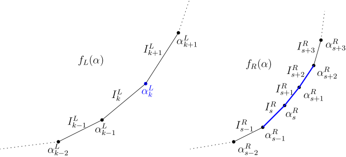
Figure 4: Illustration of situation in Claim 4 with the two functions $f_{L}(\alpha)$, $f_{R}(\alpha)$ and their critical points. Note that the slopes of of $f_{R}(\alpha)$ in intervals $I^{R}_{s},I^{R}_{s+1},I^{R}_{s+2}$ fall between the slopes of $I^{L}_{k},I^{L}_{k+1}$ so ${\cal R}^{L}_{k}=\{s,s+1,s+2\}.$

See Figure 4.

In what follows, it is assumed that $\alpha\in[a_{1}+b_{1},a_{2}+b_{2}]$. By the continuity of $f_{L}$ and $f_{R}$ and the compactness of $B$, $M(\alpha)$ is well-defined and continuous.

Label the critical points of $f_{L}$ in $[a_{1},a_{2}]$ as $\alpha^{L}_{1}<\alpha^{L}_{2}<\cdots<\alpha_{t-1}^{L}$ and set $\alpha^{L}_{0}=a_{1}$ and $\alpha^{L}_{t}=a_{2}$. The intervals $I^{L}_{k}=[\alpha^{L}_{k-1},\alpha^{L}_{k}]$ partition $[a_{1},a_{2}]$ (note that the subintervals overlap at the critical points). Let $m^{L}_{k},\beta^{L}_{k}$ be such that

$$\forall\alpha\in I^{L}_{k},\quad f_{L}(\alpha)=m^{L}_{k}\alpha+\beta^{L}_{k}.$$

By the conditions of the lemma, $m^{L}_{1}<m^{L}_{2}<\cdots<m^{L}_{t}$.

Similarly, label the critical points of $f_{R}$ in $[b_{1},b_{2}]$ as $\alpha^{R}_{1}<\alpha^{R}_{2}<\cdots<\alpha_{u-1}^{R}$ and set $\alpha^{R}_{0}=b_{1}$ and $\alpha^{R}_{u}=b_{2}$. The intervals $I^{R}_{s}=[\alpha^{R}_{s-1},\alpha^{R}_{s}]$ similarly partition $[b_{1},b_{2}]$. Let $m^{R}_{s},\beta^{R}_{s}$ be such that

$$\forall\alpha\in I^{R}_{s},\quad f_{R}(\alpha)=m^{R}_{s}\alpha+\beta^{R}_{s}.$$

By the conditions of the lemma, $m^{R}_{1}<m^{R}_{2}<\cdots<m^{R}_{u}$.

Finally, let $\breve{I}$ denote the largest open interval contained in $I$, so $\breve{I}^{L}_{k}=(\alpha^{L}_{k-1},\alpha^{L}_{k})$ and $\breve{I}^{R}_{s}=(\alpha^{R}_{s-1},\alpha^{R}_{s}).$

Now define

$$M(y,\alpha_{1},\alpha_{2})=\max\left(f_{L}(\alpha_{1})+y,f_{R}(\alpha_{2})-y\right).$$

For fixed $\alpha$, further define

$$T(\alpha)=\Bigl{\{}(y,\alpha_{1},\alpha_{2})\,:\ y\in[\ell,r,],\ (\alpha_{1},\alpha_{2})\in B(\alpha),\,\mbox{ and }M(y,\alpha_{1},\alpha_{2})=M(\alpha)\Bigr{\}}.$$

Every $(y,\alpha_{1},\alpha_{2})\in T(\alpha)$, is called a candidate triple (for $\alpha$).

Now consider the following eight conditions:

$$\begin{array}[]{llcll}(C_{1})&y=\ell,&&(C_{2})&y=r,\\ (C_{3})&y\not\in\{\ell,r\}\mbox{ and }\alpha_{1}=a_{1},&&(C_{4})&y\not\in\{\ell,r\}\mbox{ and }\alpha_{1}=a_{2},\\ (C_{5})&y\not\in\{\ell,r\}\mbox{ and }\alpha_{2}=b_{1},&&(C_{6})&y\not\in\{\ell,r\}\mbox{ and }\alpha_{2}=b_{2},\end{array}$$

$(C7)$ At least one of $\alpha_{1}=\alpha_{k}^{L}$ or $\alpha_{2}=\alpha_{s}^{R}$ is true for some $k$ or $s$
                   and $(y,\alpha_{1},\alpha_{2})$ does not satisfy $(C_{1})-(C_{6})$,
$(C_{8})$ None of $(C_{1})-(C_{7})$ is satisfied.

Similar to the proof of Lemma 17 a function $\bar{M}(\alpha)$ is called a witness for condition $(C_{i})$ if

$$\bar{M}(\alpha)\left\{\begin{array}[]{ll}=M(\alpha)&\mbox{if there exists $(y,\alpha_{1},\alpha_{2})\in T(\alpha)$ that satisfies condition $C_{i}$},\\ \geq M(\alpha)&\mbox{if there does not exist any $(y,\alpha_{1},\alpha_{2})\in T(\alpha)$ that satisfies condition $C_{i}$}.\\ \end{array}\right.$$

By default, if no $(y,\alpha_{1},\alpha_{2})\in T(\alpha)$ exists that satisfies condition $(C_{i})$ and $\bar{M}(\alpha)$ is undefined, we will assume that $\bar{M}(\alpha)=\infty$ (so that it is trivially a witness).

Every candidate triple must satisfy at least one of conditions $(C_{1})$-$(C_{8})$; Claim 7 later will show that $(C_{8})$ is superfluous and that every $\alpha$ will be witnessed by some $(C_{i})$, $i\leq 7.$ Similar to the proof of Lemma 18, we construct $O(n)$-size piecewise linear witness functions for each $(C_{i})$, $i\leq 7,$ and then take their minimum. The main work will be for $(C_{7})$, where it is not a-priori obvious that the witness function has size $O(n).$

Set

$$M^{(1)}:[a_{1}+b_{1},a_{2}+b_{2}]\rightarrow\Re, M^{(1)}(\alpha)=\min_{(\alpha_{1},\alpha_{2})\in B(\alpha)}M(\ell,\alpha_{1},\alpha_{2}),$$ (25)

$$M^{(2)}:[a_{1}+b_{1},a_{2}+b_{2}]\rightarrow\Re, M^{(2}(\alpha)=\min_{(\alpha_{1},\alpha_{2})\in B(\alpha)}M(r,\alpha_{1},\alpha_{2}).$$ (26)

Direct application of Lemmas 16 and 17 yields that both $M^{(1)}$ and $M^{(2)}$ are good functions that can be constructed in $O(n)$ time and are, respectively, witnesses for conditions $(C_{1})$ and $(C_{2}).$

Now define

$$y(\alpha_{1},\alpha_{2})=\frac{1}{2}\left(f_{R}(\alpha_{2})-f_{L}(\alpha_{1})\right).$$

Note that

$$f_{L}(\alpha_{1})+y(\alpha_{1},\alpha_{2})=\frac{1}{2}\left(f_{R}(\alpha_{2})+f_{L}(\alpha_{1})\right)\\ =f_{R}(\alpha_{2})-y(\alpha_{1},\alpha_{2})$$

so

$$M(y(\alpha_{1},\alpha_{2}),\alpha_{1},\alpha_{2})=\frac{1}{2}\left(f_{R}(\alpha_{2})+f_{L}(\alpha_{1})\right).$$ (27)

Claim 1: If $(y,\alpha_{1},\alpha_{2})\in T(\alpha)$, then

$$y=\left\{\begin{array}[]{ll}l&\mbox{ if $y(\alpha_{1},\alpha_{2})\leq l$}\\ y(\alpha_{1},\alpha_{2})&\mbox{ if $l\leq y(\alpha_{1},\alpha_{2})\leq r$}\\ r&\mbox{ if $y(\alpha_{1},\alpha_{2})\geq r$}\end{array}\right.$$ (28)

There are three cases to check.

Case (a): Assume $l\leq y(\alpha_{1},\alpha_{2})\leq r$: If $y>y(\alpha_{1},\alpha_{2})$, then

$$M(y,\alpha_{1},\alpha_{2})\geq f_{L}(\alpha_{1})+y>M(y(\alpha_{1},\alpha_{2}),\alpha_{1},\alpha_{2}).$$

Similarly, if $y<y(\alpha_{1},\alpha_{2})$, then

$$M(y,\alpha_{1},\alpha_{2})\geq f_{R}(\alpha_{2})-y>M(y(\alpha_{1},\alpha_{2}),\alpha_{1},\alpha_{2}).$$

Thus, $(y,\alpha_{1},\alpha_{2})\in T(\alpha)$ implies $y=y(\alpha_{1},\alpha_{2}).$

Case (b): Assume $y(\alpha_{1},\alpha_{2})\leq l:$ If $l<y$, then

$$M(y,\alpha_{1},\alpha_{2}) \geq f_{L}(\alpha_{1})+y$$

$$> f_{L}(\alpha_{1})+l$$

$$\geq f_{L}(\alpha_{1})+y(\alpha_{1},\alpha_{2})$$

$$= f_{R}(\alpha_{2})-y(\alpha_{1},\alpha_{2})$$

$$\geq f_{R}(\alpha_{2})-l.$$

Thus

$$M(y,\alpha_{1},\alpha_{2})>\max\left(f_{L}(\alpha_{1})+l,\,f_{R}(\alpha_{2})-l\right)=M(l,\alpha_{1},\alpha_{2}).$$

So $(y,\alpha_{1},\alpha_{2})\in T(\alpha)$ implies $y=l.$

Case (c): Assume $y(\alpha_{1},\alpha_{2})\geq r:$ If $y<r$ then

$$M(y,\alpha_{1},\alpha_{2}) \geq f_{R}(\alpha_{2})-y$$

$$> f_{R}(\alpha_{2})-r$$

$$\geq f_{R}(\alpha_{2})-y(\alpha_{1},\alpha_{2})$$

$$= f_{L}(\alpha_{1})+y(\alpha_{1},\alpha_{2})$$

$$\geq f_{L}(\alpha_{1})+r.$$

Thus

$$M(y,\alpha_{1},\alpha_{2})>\max\left(f_{L}(\alpha_{1})+r,\,f_{R}(\alpha_{2})-r\right)=M(r,\alpha_{1},\alpha_{2}).$$

So $(y,\alpha_{1},\alpha_{2})\in T(\alpha)$ implies $y=r.$

This completes the proof of Claim 1.

Claim 2: If $(y,\alpha_{1},\alpha_{2})\in T(\alpha)$ and $y\not\in\{\ell,r\}$ then

$$y=y(\alpha_{1},\alpha_{2})\quad\mbox{and}\quad M(y,\alpha_{1},\alpha_{2})=\frac{1}{2}\left(f_{L}(\alpha_{1})+f_{R}(\alpha_{2})\right).$$

Claim 2 follows directly from Claim 1 and Equation 27.

Now define (for the appropriate ranges)

$$\begin{array}[]{ccccc}M^{(3)}(\alpha)&=&M\left(y(a_{1},\alpha-a_{1}),a_{1},\alpha-a_{1}\right)&=&\frac{1}{2}\left(f_{L}(a_{1})+f_{R}(\alpha-a_{1})\right).\\ M^{(4)}(\alpha)&=&M\left(y(a_{2},\alpha-a_{2}),a_{2},\alpha-a_{2}\right)&=&\frac{1}{2}\left(f_{L}(a_{2})+f_{R}(\alpha-a_{2})\right).\\ M^{(5)}(\alpha)&=&M\left(y(\alpha-b_{1},b_{1}),\alpha-b_{1},b_{1}\right)&=&\frac{1}{2}\left(f_{L}(\alpha-b_{1})+f_{R}(b_{1})\right).\\ M^{(6)}(\alpha)&=&M\left(y(\alpha-b_{2},b_{2}),\alpha-b_{2},b_{2}\right)&=&\frac{1}{2}\left(f_{L}(\alpha-b_{2})+f_{R}(b_{2})\right).\end{array}$$

Multiple applications of Lemma 16 show that $M^{(i)}$ $i=3,4,5,6$ are all positive good functions that can be constructed in $O(n)$ time.

From Claims 1 and 2, if $(y,\alpha_{1},\alpha_{2})\in T(\alpha)$ satisfies condition $(C_{i})$ for $i=3,4,5,6$, then $M(\alpha)=M^{(i)}(\alpha)$. Thus $M^{(i)}$ $i=3,4,5,6$ are witnesses for condition $(C_{i}).$

We now consider when a candidate triple $(y,\alpha_{1},\alpha_{2})\in T(\alpha)$ satisfies condition $(C_{7}).$ We first derive properties that will permit constructing this witness function quickly.

Claim 3: Suppose $(y,\alpha_{1},\alpha_{2})\in T(\alpha)$ does not satisfy any of conditions $(C_{1})-(C_{6})$

• Further suppose that $\alpha_{1}=\alpha_{k}^{L}$ is a critical point of $f_{L}$ and $\alpha_{2}\in I^{R}_{s}=\left[\alpha^{R}_{s-1},\alpha^{R}_{s}\right]$. Then

  • if $\alpha_{2}>\alpha^{R}_{s-1}$, then $m^{R}_{s}\leq m^{L}_{k+1}$

  • if $\alpha_{2}<\alpha^{R}_{s}$, then $m^{L}_{k}\leq m^{R}_{s}$.

  • If $\alpha_{2}\in\breve{I}^{R}_{s}$ then $m^{L}_{k}\leq m^{R}_{s}\leq m^{L}_{k+1}.$

• Now, further suppose $(y,\alpha_{1},\alpha_{2})\in T(\alpha)$ does not satisfy any of conditions $(C_{1})-(C_{6})$, $\alpha_{2}=\alpha_{s}^{R}$ is a critical point of $f_{R}$ and $\alpha_{1}\in I^{L}_{k}=[\alpha^{L}_{k-1},\alpha^{L}_{k}]$. Then

  • if $\alpha_{1}>\alpha^{L}_{k-1},$ then $m^{L}_{k}\leq m^{R}_{s+1}$.

  • if $\alpha_{1}<\alpha^{L}_{k},$ then $m^{R}_{s}\leq m^{L}_{k}$.

  • If $\alpha_{1}\in\breve{I}^{L}_{k}$ then $m^{R}_{s}\leq m^{L}_{k}\leq m^{R}_{s+1}.$

We prove (A). The proof of (B) is symmetric.

From Claim 2 and $(y,\alpha_{1},\alpha_{2})$ not satisfying $(C_{1})$ and $(C_{2}),$ we have $y=y(\alpha_{1},\alpha_{2})$ and $\ell<y<r.$ From $(y,\alpha_{1},\alpha_{2})$ not satisfying any of $(C_{3})-(C_{6}),$ we can find $\epsilon$ small enough that

$$\forall\alpha^{\prime}_{1}\in[\alpha_{1}-\epsilon,\alpha_{1}+\epsilon],\ \forall\alpha^{\prime}_{2}\in[\alpha_{2}-\epsilon,\alpha_{2}+\epsilon],\quad\ell<y(\alpha^{\prime}_{1},\alpha^{\prime}_{2})<r.$$

Thus, from Claims 1 and 2,

$$M(y,\alpha_{1}+\epsilon,\alpha_{2}-\epsilon) = \frac{1}{2}\left(f_{L}(\alpha_{1}+\epsilon)+f_{R}(\alpha_{2}-\epsilon)\right),$$

$$M(y,\alpha_{1}-\epsilon,\alpha_{2}+\epsilon) = \frac{1}{2}\left(f_{L}(\alpha_{1}-\epsilon)+f_{R}(\alpha_{2}+\epsilon)\right).$$

From $\alpha_{1}=\alpha_{k}^{L}$, for small enough $\epsilon,$

$$f_{L}(\alpha_{1}-\epsilon)=f_{L}(\alpha_{1})-m^{L}_{k}\epsilon,\quad\mbox{and}\quad f_{L}(\alpha_{1}+\epsilon)=f_{L}(\alpha_{1})+m^{L}_{k+1}\epsilon,$$

To see (i), note that if if $\alpha_{2}>\alpha^{R}_{s-1}$, then for small enough $\epsilon>0,$

$$f_{R}(\alpha_{2}-\epsilon)=f_{R}(\alpha_{2})-m^{R}_{s}\epsilon.$$

This implies that if $m^{R}_{s}>m^{L}_{k+1},$

$$M(y,\alpha_{1}+\epsilon,\alpha_{2}-\epsilon) = \frac{1}{2}\left(f_{L}(\alpha_{1}+\epsilon)+f_{R}(\alpha_{2}-\epsilon)\right),$$

$$= \frac{1}{2}\left(f_{L}(\alpha_{1})+f_{R}(\alpha_{2})\right)+\frac{\epsilon}{2}\left(m^{L}_{k+1}-m^{R}_{s}\right)$$

$$< \frac{1}{2}\left(f_{L}(\alpha_{1})+f_{R}(\alpha_{2})\right)=M(y,\alpha_{1},\alpha_{2})$$

contradicting the fact that $(y,\alpha_{1},\alpha_{2})$ is a candidate triple. Thus, $m^{R}_{s}\leq m^{L}_{k+1}$.

To see (ii), note that if $\alpha_{2}<\alpha^{R}_{s}$, then for small enough $\epsilon>0,$

$$f_{R}(\alpha_{2}+\epsilon)=f_{R}(\alpha_{2})+m^{R}_{s}\epsilon.$$

This implies that if $m^{R}_{s}<m^{L}_{k}$,

$$M(y,\alpha_{1}-\epsilon,\alpha_{2}+\epsilon) = \frac{1}{2}\left(f_{L}(\alpha_{1}-\epsilon)+f_{R}(\alpha_{2}+\epsilon)\right),$$

$$= \frac{1}{2}\left(f_{L}(\alpha_{1})+f_{R}(\alpha_{2})\right)+\frac{\epsilon}{2}\left(m^{R}_{s}-m^{L}_{k}\right)$$

$$< \frac{1}{2}\left(f_{L}(\alpha_{1})+f_{R}(\alpha_{2})\right)=M(y,\alpha_{1},\alpha_{2})$$

again contradicting the fact that $(y,\alpha_{1},\alpha_{2})$ is a candidate triple. Thus $m^{L}_{k}\leq m^{R}_{s}.$

Point (iii) follows from combining points (i) and (ii), completing the proof of Claim 3(A).

Claim 4: Suppose $(y,\alpha_{1},\alpha_{2})\in T(\alpha)$ satisfies condition $(C_{7})$. For each $\alpha_{k}^{L}$ and $\alpha_{s}^{R},$ define

$${\cal R}^{L}_{k}=\left\{s:m^{L}_{k}\leq m^{R}_{s}\leq m^{L}_{k+1}\right\},\quad{\cal R}^{R}_{s}=\left\{k:m^{R}_{s}\leq m^{L}_{k}\leq m^{R}_{s+1}\right\}$$

and

$${\cal I}^{L}_{k}=\bigcup_{s\in{\cal R}^{L}_{k}}I_{s}^{R},\quad{\cal I}^{R}_{s}=\bigcup_{k\in{\cal R}^{R}_{s}}I_{k}^{L}.$$

Then

• If $\alpha_{1}=\alpha_{k}^{L}$ is a critical point of $f_{L}$ then
  either $\alpha_{2}\in{\cal I}^{L}_{k}$ or  $\alpha_{2}=\alpha_{s}^{R}$ (a critical point of $f_{R}$) and $\alpha_{1}\in{\cal I}^{R}_{s}.$

• If $\alpha_{2}=\alpha_{s}^{R}$ is a critical point of $f_{R}$
  then either $\alpha_{1}\in{\cal I}^{R}_{s}$ or  $\alpha_{1}=\alpha_{k}^{L}$ (a critical point of $f_{L}$) and $\alpha_{2}\in{\cal I}^{R}_{k}.$

We prove (A). The proof of (B) is symmetric.

Suppose that $(y,\alpha_{1},\alpha_{2})\in T(\alpha)$ satisfies condition $(C_{7})$ with $\alpha_{1}=\alpha_{k}^{L}$. If $\alpha_{2}\in\breve{I}^{R}_{s}$, then by Claim 3(A)(iii), $I^{R}_{s}\subseteq{\cal I}^{L}_{k}$ and the claim is correct.

Otherwise, $\alpha_{2}$ is a critical point, i.e.,  $\alpha_{2}=\alpha^{R}_{s}$ for some $s$. Claims 3(A) (i) and (ii) then imply

$$m^{R}_{s}\leq m^{L}_{k+1}\quad\mbox{and}\quad m^{R}_{s+1}\geq m^{L}_{k}.$$

If $m^{L}_{k}\leq m^{R}_{s}$ then $\alpha_{2}\in I^{R}_{s}\subseteq{\cal I}^{L}_{k}$ and the claim is correct. Otherwise $m^{R}_{s}<m^{L}_{k}\leq m^{R}_{s+1}$ and $\alpha_{1}\in I^{L}_{k}\subseteq{\cal I}^{R}_{s}$ and the claim is correct.

The decomposition above permits constructing a compact function to witness condition $(C_{7})$. It will match each critical point of $f_{L}(\alpha)$ ($f_{R}(\alpha)$) to its associated interval in $f_{R}(\alpha)$ ($f_{L}(\alpha)$).

Before continuing, we introduce the following useful notation. If $I=[a,b]$ let $\alpha+I$ denote the interval $[a+\alpha,b+\alpha].$ We say that $[a_{1},b_{1}]=I_{1}<I_{2}=[a_{2},b_{2}]$ if $b_{1}<a_{2}$ and $I_{1}\leq I_{2}$ if $b_{1}\leq a_{2}.$

It would be elegantly convenient for the later proof if the $\alpha^{L}_{k}+I^{R}_{s}$ with $s\in{\cal R}^{L}_{k}$ were all disjoint. Unfortunately, this is not true. The best that can be proven is the next claim (which suffices for our purposes).

Claim 5:

• Let $k_{1}<k_{2}$ and $s_{1}\in{\cal R}^{L}_{k_{1}}$ and $s_{2}\in{\cal R}^{L}_{k_{2}}$ such that $I=(\alpha_{k_{1}}^{L}+I_{s_{1}}^{R})\cap(\alpha_{k_{2}}^{L}+I_{s_{2}}^{R})\not=\phi.$
  Then $k_{2}=k_{1}+1.$

• Let $s_{1}<s_{2}$ and $k_{1}\in{\cal R}^{R}_{s_{1}}$ and $k_{2}\in{\cal R}^{R}_{s_{2}}$ such that $I=(\alpha_{s_{1}}^{R}+I_{k_{1}}^{L})\cap(\alpha_{s_{2}}^{R}+I_{k_{2}}^{L})\not=\phi.$
  Then $s_{2}=s_{1}+1$.

We prove (A). The proof of (B) is symmetric.

Since $m_{k_{1}+1}^{L}\leq m_{k_{2}}^{L}$, by definition $s_{1}\leq s_{2}$. If $s_{1}<s_{2}$, then $I_{s_{1}}^{R}\leq I_{s_{2}}^{R}$, and as $\alpha_{k_{1}}^{L}<\alpha_{k_{2}}^{L}$, we get $\alpha_{k_{1}}^{L}+I_{s_{1}}^{R}<\alpha_{k_{2}}^{L}+I_{s_{2}}^{R}$ so $I=\emptyset.$ Thus, we may assume $s_{1}=s_{2}.$

From the definition of ${\cal R}^{L}_{k}$, $m^{R}_{s_{1}}\leq m^{L}_{k_{1}+1}\leq m^{L}_{k_{2}}\leq m^{R}_{s_{2}}$. Since $s_{1}=s_{2},$ $k_{2}=k_{1}+1.$

Claim 6: Define

$$h^{L}_{k}(\alpha)=M\left(y(\alpha_{k}^{L},\alpha-\alpha_{k}^{L}),\alpha_{k}^{L},\alpha-\alpha_{k}^{L}\right)=\frac{1}{2}\left(f_{L}(\alpha_{k}^{L})+f_{R}(\alpha-\alpha_{k}^{L})\right) \mbox{if }\ \alpha\in\alpha_{k}^{L}+{\cal I}^{L}_{k},$$

$$h^{R}_{s}(\alpha)=M\left(y(\alpha-\alpha_{s}^{R},\alpha_{s}^{R}),\alpha-\alpha_{s}^{R},\alpha_{s}^{R}\right)=\frac{1}{2}\left(f_{L}(\alpha-\alpha_{s}^{R})+f_{R}(\alpha_{s}^{R})\right) \mbox{if }\ \alpha\in\alpha_{s}^{R}+{\cal I}^{R}_{s},$$

where the functions have value $\infty$ outside their specified domains. Further set

$$H^{L}(\alpha)=\min_{1\leq k<t}h^{L}_{k}(\alpha),\quad H^{R}(\alpha)=\min_{1\leq s<u}h^{R}_{s}(\alpha)\quad\mbox{and}\quad M^{(7)}(\alpha)=\min\left(H^{L}(\alpha),\,H^{R}(\alpha)\right).$$

Then $M^{(7)}(\alpha)$ is a piecewise linear function with positive slopes that is a witness to condition $(C_{7})$ and can be built in $O(n)$ time.

To prove this claim, first note that by definition, $\forall\alpha,$ $M^{(7)}(\alpha)\geq M(\alpha)$. Now, let $(y,\alpha_{1},\alpha_{2})$ be a candidate triple for $\alpha$ that satisfies condition $(C_{7})$. This implies that either $\alpha_{1}=\alpha^{L}_{k}$ for some $k,$ $\alpha_{2}=\alpha^{R}_{s}$ for some $s$ or both at once.

Assume that $\alpha_{1}=\alpha^{L}_{k}$ and set $\alpha_{2}=\alpha-\alpha_{1}.$ From Claim 4 and Claim 2, one of the following two events must occur.

• $\alpha_{2}\in{\cal I}^{R}_{s}$, and thus $h^{L}_{k}(\alpha)=M(y(\alpha_{1},\alpha_{2}),\alpha_{1},\alpha_{2})=M(\alpha)$ or

• $\alpha_{2}=\alpha_{s}^{R}$ is a critical point of $f_{R}$ and $\alpha_{1}\in{\cal I}^{R}_{s}$ and thus $h_{s}^{R}(\alpha)=M(y(\alpha_{1},\alpha_{2}),\alpha_{1},\alpha_{2})=M(\alpha)$

Thus, $M^{(7)}(\alpha)=M(\alpha)$. The proof that $M^{(7)}(\alpha)=M(\alpha)$ if we assume $\alpha_{2}=\alpha^{R}_{s}$ is symmetric. This proves that $M^{(7)}(\alpha)$ is a witness to condition $(C_{7})$.

We now show how to construct $H^{L}(\alpha)$ in $O(n)$ time (and that it has $O(n)$ critical points).

To start, set $I_{k}=\alpha_{k}^{L}+{\cal I}^{L}_{k},$ the domain of $h^{L}_{k}(\alpha).$ Let $\ell_{k},r_{k}$ be such that $I_{k}=[\ell_{k},r_{k}]$. Note that $I_{k}$ contains $|{\cal R}^{L}_{k}|+1$ critical points. so each $h^{L}_{k}(\alpha)$ can be built in time $O(|{\cal R}^{L}_{k}|+1).$ Furthermore, since a critical point of $H^{L}(\alpha)$ must be a critical point of one of the $I_{k}$, $H^{L}(\alpha)$ has $O\left(\sum_{k}(|{\cal R}^{L}_{k}|+1)\right)=O(n)$ critical points.

To continue, note that by construction, $\ell_{k}\leq\ell_{k+1},$ $r_{k}\leq r_{k+1}$ and, from Claim 5, $r_{k-1}<\ell_{k+1}.$

For $j<t$, define $H_{j}^{L}(\alpha)=\min\limits_{1\leq k\leq j}h^{L}_{k}(\alpha).$ Its domain is $D_{j}=\cup_{1\leq k\leq j}I_{j}=D_{j-1}\cup[\ell_{j},r_{j}]$.

Set $H_{1}^{L}(\alpha)=h^{L}_{1}(\alpha).$ Now assume that $H_{j}^{L}$ is known. We will build $H_{j+1}^{L}$ from $H_{j}^{L}$. There are two possible cases.

In the first case, $r_{j}<\ell_{j+1}.$ Then $D_{j}<I_{j+1}$ so we can just concatenate $I_{j+1}$ (along with the associated function information of $h^{L}_{j+1}(\alpha)$) to the end of $D_{j}$. This takes $O(|{\cal R}^{L}_{j+1}|+1)$ time.

In the second case, $r_{j}\geq\ell_{j+1}.$ First note that, since $r_{k-1}<\ell_{k+1}$, $D_{j-1}\cap I_{j+1}=\emptyset.$ Thus $D_{j}\cap I_{j+1}=I_{j}\cap I_{J+1}=[\ell_{j+1},r_{j}]$ and

$$H_{j+1}^{L}(\alpha)=\begin{cases}H_{j}^{L}(\alpha)&\mbox{if $\alpha\in D_{j-1}\cup[\ell_{j},\ell_{j+1})$}\\ \min(h_{j}(\alpha),h_{j+1}(\alpha))&\mbox{if $\alpha\in I_{j}\cap I_{j+1}=[\ell_{j+1},r_{j}]$}\\ h_{j+1}(\alpha)&\mbox{if $\alpha\in(r_{j},r_{j+1}]$}\end{cases}$$

Since $D_{j-1}\cap I_{j+1}=\emptyset,$ the critical points that define $D_{j}$ in $[\ell_{j+1},r_{j}]$ are all critical points in $I_{j}$. Thus $H_{j}^{L}(\alpha)$ defined on $D_{j}$ can be trimmed back to only being defined on $D_{j-1}\cup[\ell_{j},\ell_{j+1})$ in $O(|{\cal R}^{L}_{j}|+1)$ time. This yields $H_{j+1}^{L}(\alpha)$ defined on $D_{j-1}\cup[\ell_{j},\ell_{j+1})$ .

$H_{j+1}^{L}(\alpha)$ defined on $[\ell_{j+1},r_{j}]$ can be constructed in $O(|{\cal R}^{L}_{j}|+|{\cal R}^{L}_{j+1}|+1)$ time.

$H_{j+1}^{L}(\alpha)=h_{j+1}(\alpha)$ defined on $(r_{j},r_{j+1}]$ can be constructed in $O(|{\cal R}^{L}_{j+1}|+1)$ time.

Concatenating the three pieces (which only intersect at their endpoints) requires only $O(1)$ more time and yields the full description of $H_{j+1}^{L}(\alpha)$.

We have therefore just shown that, in both cases, the time required to construct $H_{j+1}^{L}(\alpha)$ from $H_{j}^{L}(\alpha)$ is $O(|{\cal R}^{L}_{j}|+|{\cal R}^{L}_{j+1}|+1).$

Thus, the total time to construct $H^{L}(\alpha)=H_{t-1}^{L}(\alpha)$ is

$$O\left(\sum_{1\leq k<t}\left(|{\cal R}^{L}_{j}|+|{\cal R}^{L}_{j+1}|+1\right)\right)=O(t)=O(n).$$

A similar argument shows that $H^{R}(\alpha)$ can also be built in $O(n)$ time and has $O(n)$ critical points. Thus, the piecewise linear function $M^{(7)}(\alpha)$ with its critical points in sorted order can be built in $O(n)$ time. Since both $H^{L}(\alpha)$ and $H^{R}(\alpha)$ have $O(n)$ critical points, $M^{(7)}(\alpha)$ does as well.

Furthermore, since all the individual $h_{k}^{L}(\alpha)$ and $h_{s}^{R}(\alpha)$ have positive slopes, $M^{(7)}(\alpha)$ does as well. This completes the proof of Claim 6.

Claim 7: Suppose $(y,\alpha_{1},\alpha_{2})\in T(\alpha)$ satisfies condition $(C_{8})$. Then there exists another $(y^{\prime},\alpha^{\prime}_{1},\alpha^{\prime}_{2})\in T(\alpha)$ that satisfies at least one of the conditions $(C_{1})-(C_{7})$.

Because $(y,\alpha_{1},\alpha_{2})$ does not satisfy any of conditions $(C_{1})-(C_{7})$, $\alpha_{1}$ is not a critical point of $f_{L}$, $\alpha_{2}$ is not a critical point of $f_{R}$ and $l<y(\alpha_{1},\alpha_{2})<r$ since otherwise, either $(l,\alpha_{1},\alpha_{2})$ or $(r,\alpha_{1},\alpha_{2})\in T(\alpha)$ and we are done. Furthermore, there exist $k,s$ and $\epsilon>0$ such that

$$[\alpha_{1}-\epsilon,\alpha_{1}+\epsilon]\subseteq I^{L}_{k},\,\quad\mbox{and}\quad[\alpha_{2}-\epsilon,\alpha_{2}+\epsilon]\subseteq I^{R}_{s}.$$ (29)

and at least one of the following facts is true:
(a) at least one of the two points $\alpha_{1}\pm\epsilon$ is a critical point of $f_{L}$ (b) $\alpha_{1}-\epsilon=a_{1},$ (c) $\alpha_{1}+\epsilon=a_{2},$ (d) at least one of the two points $\alpha_{2}\pm\epsilon$ is a critical point of $f_{R}$ (e) $\alpha_{2}-\epsilon=b_{1},$ (f) $\alpha_{2}+\epsilon=b_{2}.$

Recall that Equation 29 implies

$$\forall\alpha_{1}^{\prime}\in[\alpha_{1}-\epsilon,\alpha_{1}+\epsilon],\,f_{L}(\alpha_{1}^{\prime})=m^{L}_{k}\alpha_{1}^{\prime}+b^{L}_{k}\quad\mbox{and}\quad\forall\alpha_{2}^{\prime}\in[\alpha_{2}-\epsilon,\alpha_{2}+\epsilon],\,f_{R}(\alpha_{2}^{\prime})=m^{R}_{s}\alpha_{2}^{\prime}+b^{R}_{s}.$$

Suppose that $m^{L}_{k}\not=m^{R}_{s}$. Without loss of generality, assume that $m^{L}_{k}>m^{R}_{s}$. Because neither condition $(C_{2})$, $(C_{3})$ hold, we can choose $\epsilon^{\prime}<\epsilon$ small enough that

$$y(\alpha_{1}-\epsilon^{\prime},\alpha_{2}+\epsilon^{\prime})=y(\alpha_{1},\alpha_{2})-\frac{\epsilon^{\prime}}{2}(m^{L}_{k}-m^{R}_{s})$$

satisfies

$$l\leq y(\alpha_{1}-\epsilon^{\prime},\alpha_{2}+\epsilon^{\prime})\leq r.$$

But then

$$M(y(\alpha_{1}-\epsilon^{\prime},\alpha_{2}+\epsilon^{\prime}),\alpha_{1}-\epsilon^{\prime},\alpha_{2}+\epsilon^{\prime})=M(y(\alpha_{1},\alpha_{2}),\alpha_{1},\alpha_{2})-\frac{\epsilon^{\prime}}{2}(m^{L}_{k}-m^{R}_{s})<M(y(\alpha_{1},\alpha_{2}),\alpha_{1},\alpha_{2})=M(\alpha)$$

contradicting the definition of $T(\alpha).$ So this case can not occur and $m^{L}_{k}=m^{R}_{s}$.

Now $m^{L}_{k}=m^{R}_{s}$ implies that

$$y(\alpha_{1}-\epsilon,\alpha_{2}+\epsilon)=y(\alpha_{1},\alpha_{2})=y(\alpha_{1}+\epsilon,\alpha_{2}-\epsilon)$$

and

$$M(y(\alpha_{1}-\epsilon,\alpha_{2}+\epsilon),\alpha_{1}-\epsilon,\alpha_{2}+\epsilon)=M(y,\alpha_{1},\alpha_{2})=M(y(\alpha_{1}+\epsilon,\alpha_{2}-\epsilon),\alpha_{1}+\epsilon,\alpha_{2}-\epsilon).$$

Since at least one of facts (a)-(f) is true, this constructs a candidate triple for $(y(\alpha_{1}+\epsilon,\alpha_{2}-\epsilon),\alpha_{1}-\epsilon,\alpha_{2}+\epsilon)\in T(\alpha)$ that satisfies at least one of conditions $(C_{1})-(C_{7})$, thus proving Claim 7.

Claim 8: $M(\alpha)$ is a good function that can be constructed in $O(n)$ time.

From Claim 7, for every $\alpha$, there exists a candidate triple for $\alpha$ that satisfies at least one of conditions $(C_{1})-(C_{7})$. We have already seen that, for each $i=1,\ldots 7,$ $M^{(i)}(\alpha)$ is a witness to condition $(C_{i})$. Thus $M(\alpha)=\min_{1\leq i\leq 7}M^{(i)}(\alpha).$

Each $M^{(i)}(\alpha)$, $i\leq 6$ is a good function that can be built in $O(n)$ time. From Claim 6, $M^{(7)}(\alpha)$ is a piecewise linear function of size $O(n)$ that can be built in $O(n)$ time (it might not be good since it might not be continuous). Thus, from Lemma 16, $M(\alpha)$ is a piecewise linear function that can be built in $O(n)$ time, all of whose slopes are positive.

$M(\alpha)$ being good follows from the continuity of $M$ (noted at the start of the proof). ∎

8 Conclusion and Possible Extensions

This paper provided an $O(n^{4}\log n)$ time algorithm for solving the 1-sink location minmax regret problem on a dynamic path network with general capacities. To the best of our knowledge, this is the first polynomial time algorithm for solving any sink location minmax regret problem with general capacities for any type of graph and any number of sinks.

While polynomial, this running time is quite high and an obvious direction for future research would be to speed it up. One possible approach would be to note that Section 4 shows that the problem can be solved in $O(U(n)n^{2}\log n)$ time where $U(n)$ is the time required to calculate $G_{i,j}(x)$ and the other functions introduced in Definition 12. The second half of the paper, Sections 6 and 7, develop a machinery for proving that $U(n)=O(n^{2})$.

Any improvement to $U(n)$ would improve the algorithm. We note without details that an even more intricate analysis than that presented here could evaluate $G_{i,j}(x)$ and $G_{j}(x)$ in $O(n)$ rather than $O(n^{2})$ time. This analysis uses amortization to show that not only is $M^{(u)}_{i}(x)$ a good function of size $O(n)$ for each $u,$ but the full $M_{i}(x)$ has size $O(n)$ as well (the analysis presented in this paper only shows that $M_{i}(x)$ has size $O(n^{2})$). Straightforward modifications of Lemmas 24 and 25 would then evaluate $G_{i,j}(x)$ and $G_{j}(x)$ in $O(n)$ time.

The reason that this approach can not (yet) be used to derive a better bound on $U(n)$ is that the amortization argument strongly uses the fact that $M_{i}(x)$ is a piecewise linear function of only one varying parameter. This permits showing that the different $M^{(u)}_{i}(x)$ can not all be large and thus $M_{i}(x)=\max_{u}M^{(u)}_{i}(x)$ is not composed of many pieces. The amortization argument fails for $M_{i,j}(x)$ though, because $M_{i,j}(x)$ is fundamentally a piecewise linear function in two varying parameters. Thus, it would not be possible to use this to prove that $U(n)=O(n).$

This failure does highlight that a possible method of improving the algorithm would be developing a different approach to showing that $M_{i,j}(x)$ has size $O(n)$. An $O(n)$ time construction of $M_{i,j}(x)$ (it is unknown whether this is possible) would immediately imply that $U(n)=O(n)$ and lead to an $O(n^{3}\log n)$ time algorithm.

It would also be interesting to try to solve the $k$-sink location minmax regret problem on a dynamic path with general capacities for any $k>1.$ The corresponding algorithms [21, 7, 3] in the uniform capacity case strongly utilized the combinatorial structure of worst case solutions that were independent of the actual scenario weight values. Because the worst case scenarios in the general capacity case are dependent on the actual weight values, those techniques can not be easily transferred.

Similarly, it would also be interesting to try to solve the $1$-sink location minmax regret problem on a dynamic tree with general capacities. The corresponding regret problem with uniform capacities [19, 7] used the fact that the optimization (not regret) problem on a tree with uniform capacities could be transformed to a path problem. This reduction is no longer valid in the general capacity case and so those techniques can also not be easily transferred here.

References

- Aissi et al. [2009] H. Aissi, C. Bazgan, and D. Vanderpooten. Min–max and min–max regret versions of combinatorial optimization problems: A survey. European Journal of Operational Research, 197(2):427–438, 2009.
- Aronson [1989] Jay E Aronson. A survey of dynamic network flows. Annals of Operations Research, 20(1):1–66, 1989.
- Arumugam et al. [2019] Guru Prakash Arumugam, John Augustine, Mordecai J Golin, and Prashanth Srikanthan. Minmax regret k-sink location on a dynamic path network with uniform capacities. Algorithmica, 81:3534–3585, 2019.
- Averbakh and Berman [1997] I. Averbakh and O. Berman. Minimax regret p-center location on a network with demand uncertainty. Location Science, 5(4):247–254, 1997.
- Averbakh and Berman [2003] Igor Averbakh and Oded Berman. An improved algorithm for the minmax regret median problem on a tree. Networks: An International Journal, 41(2):97–103, 2003.
- Benkoczi et al. [2019] Robert Benkoczi, Binay Bhattacharya, Yuya Higashikawa, Tsunehiko Kameda, and Naoki Katoh. Minmax-regret evacuation planning for cycle networks. In International Conference on Theory and Applications of Models of Computation, pages 42–58. Springer, 2019.
- Bhattacharya and Kameda [2015] B. Bhattacharya and T. Kameda. Improved algorithms for computing minmax regret sinks on dynamic path and tree networks. Theoretical Computer Science, 607:(411–425), 2015.
- Bhattacharya et al. [2017] B. Bhattacharya, M. J. Golin, Y. Higashikawa, T. Kameda, and N. Katoh. Improved algorithms for computing k-sink on dynamic flow path networks. In Proceedings of WADS’2017, 2017.
- Bhattacharya and Kameda [2012] Binay K. Bhattacharya and Tsunehiko Kameda. A linear time algorithm for computing minmax regret 1-median on a tree. In COCOON’2012, pages 1–12, 2012.
- Brodal et al. [2008] G. S. Brodal, L. Georgiadis, and I. Katriel. An version of the Averbakh–Berman algorithm for the robust median of a tree. Operations Research Letters, 36(1):14–18, January 2008.
- Chen and Golin [2016] Di Chen and Mordecai Golin. Sink Evacuation on Trees with Dynamic Confluent Flows. In ISAAC 2016, pages 25:1–25:13, 2016.
- Chen and Golin [2018] Di Chen and Mordecai Golin. Minmax centered k-partitioning of trees and applications to sink evacuation with dynamic confluent flows. CoRR, abs/1803.09289, 2018.
- Chen et al. [2007] J. Chen, R. D. Kleinberg, L. Lovász, R. Rajaraman, R. Sundaram, and A. Vetta. (Almost) Tight bounds and existence theorems for single-commodity confluent flows. Journal of the ACM, 54(4), jul 2007.
- Cheng et al. [2013] S.-W. Cheng, Y. Higashikawa, N. Katoh, G. Ni, and Y. Su, B.and Xu. Minimax regret 1-sink location problems in dynamic path networks. In Proceedings of TAMC’2013, pages 121–132, 2013.
- Dressler and Strehler [2010] Daniel Dressler and Martin Strehler. Capacitated Confluent Flows: Complexity and Algorithms. In Proceedings of CIAC’10, pages 347–358, 2010.
- Fleischer and Skutella [2007] Lisa Fleischer and Martin Skutella. Quickest Flows Over Time. SIAM Journal on Computing, 36(6):1600–1630, January 2007.
- Ford and Fulkerson [1958] L. R. Ford and D. R. Fulkerson. Constructing Maximal Dynamic Flows from Static Flows. Operations Research, 6(3):419–433, June 1958.
- Higashikawa et al. [2015] Y. Higashikawa, J. Augustine, S.-W. Cheng, M.J. Golin, N. Katoh, G. Ni, B. Su, and Y.F. Xu. Minimax regret 1-sink location problem in dynamic path networks. Theoretical Computer Science, 588(11):24–36, 2015.
- Higashikawa et al. [2014] Yuya Higashikawa, M. J. Golin, and Naoki Katoh. Minimax Regret Sink Location Problem in Dynamic Tree Networks with Uniform Capacity. J. Graph Algorithms Appl, 18(4):539–555, 2014.
- Kouvelis and Yu [1997] Panos Kouvelis and Gang Yu. Robust Discrete Optimization and Its Applications. Kluwer Academic Publishers, 1997.
- Li et al. [2014] Hongmei Li, Yinfeng Xu, and Guanqun Ni. Minimax regret vertex 2-sink location problem in dynamic path networks. Journal of Combinatorial Optimization, February 2014.
- Mamada et al. [2006] S. Mamada, T. Uno, K. Makino, and S. Fujishige. An algorithm for the optimal sink location problem in dynamic tree networks. Discrete Applied Mathematics, 154(16):2387–2401, 2006.
- Shepherd and Vetta [2015] F Bruce Shepherd and Adrian Vetta. The inapproximability of maximum single-sink unsplittable, priority and confluent flow problems. arXiv preprint arXiv:1504.00627, 2015.
- Wang [2014] Haitao Wang. Minmax regret 1-facility location on uncertain path networks. European Journal of Operational Research, 239(3):636–643, 2014.
- Yu et al. [2008] H-I. Yu, T-C Lin, and B-F Wang. Improved algorithms for the minmax-regret 1-center and 1-median problems. ACM Transactions on Algorithms, 4(3):1–27, June 2008.