Handling cellwise outliers by sparse regression and robust covariance

Abstract

We propose a data-analytic method for detecting cellwise outliers. Given a robust covariance matrix, outlying cells (entries) in a row are found by the cellHandler technique which combines lasso regression with a stepwise application of constructed cutoff values. The penalty term of the lasso has a physical interpretation as the total distance that suspicious cells need to move in order to bring their row into the fold. For estimating a cellwise robust covariance matrix we construct a detection-imputation method which alternates between flagging outlying cells and updating the covariance matrix as in the EM algorithm. The proposed methods are illustrated by simulations and on real data about volatile organic compounds in children.

Keywords: anomalous cells, cellHandler, detection-imputation method, least angle regression algorithm, marginal outliers.

1 Introduction

It is a fact of life that most real data sets contain outliers, that is, elements that do not fit in with the majority of the data. These outliers can be annoying errors, but may also contain valuable information. In either case, finding them is of practical importance. In statistics this is called outlier detection, and in the computer science literature it is also called anomaly detection or exception mining, see e.g. Chandola et al., (2009).

The most common paradigm is that of casewise outliers, which assumes that most cases were drawn from a certain model distribution but some other cases were not. The latter are also called rowwise outliers, since data often comes in the form of a table (matrix) in which the rows are the cases and the columns represent the variables. In computer science one often uses outlier detection methods based on Euclidean distances, which by construction are invariant for orthogonal transformations of the rows. In statistics many outlier detection methods are also invariant for affine transformations, i.e. nonsingular linear transforms combined with shifts.

The study of cellwise outliers is a more recent research topic. This is the situation where some individual cells (entries) of the data matrix deviate from what they should have been. Alqallaf et al., (2009) first formulated this paradigm. Note that cells are intimately tied to the coordinate system, whereas orthogonal or other linear transformations would change the cells. To illustrate the difference between the rowwise and cellwise approaches, consider the standard multivariate Gaussian model in dimension $d=4$ with the suspicious point $(10,0,0,0)$. By an orthogonal transformation of the data this point can be moved to $(\sqrt{50},\sqrt{50},0,0)$ or to $(5,5,5,5)$ so any orthogonally invariant rowwise detection method will treat all three situations the same way. But in the cellwise paradigm $(10,0,0,0)$ has one outlying cell, $(\sqrt{50},\sqrt{50},0,0)$ has two and $(5,5,5,5)$ has four.

For an illustration of cellwise outliers see Figure 1. It depicts part of a dataset that will be described later. The rows are cases and the columns are variables. The regular cells are shown in yellow. Red colored cells indicate that their value is higher than expected, while blue cells indicate unusually low values.

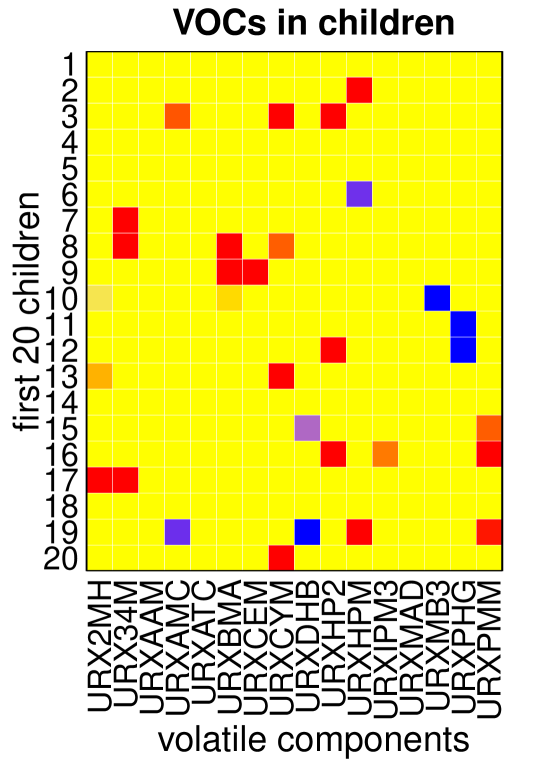
Figure 1: Illustration of cellwise outliers. Red squares indicate cells with unexpectedly high values, and blue squares indicate unusually low values. Regular cells are yellow.

When the model has substantially correlated variables the cellwise outliers need not be marginally outlying, and then it can be quite hard to detect them. Van Aelst et al., (2011) proposed one of the first methods, based on an outlyingness measure of the Stahel-Donoho type. Farcomeni, (2014) looks for the cells that, when put to missing, yield the highest Gaussian partial likelihood. Agostinelli et al., (2015) and Leung et al., (2017) use a univariate or bivariate filter on the variables to flag cellwise outliers, followed by S-estimation. Rousseeuw and Van den Bossche, (2018) predict the values of all cells and flag the observed cells that differ much from their prediction. Debruyne et al., (2019) consider rowwise outliers and ask which variables contribute the most to their outlyingness. The O3 plot of Unwin, (2019) visualizes cases that are outlying in lower dimensions.

There has also been substantial work to estimate the covariance matrix underlying the model in the presence of cellwise outliers, which will be be briefly reviewed in Section 3.1.

Most of the statistical research on cellwise outliers has focused on the FICM contamination model of Alqallaf et al., (2009) which assumes that the outlying cells come from a single distribution, and typically this distribution has all its mass in a single value $\gamma$. Here we will not restrict ourselves to that setting, and in the simulations we will allow for the cellwise outlying values to depend on which cells are contaminated, creating structured cellwise outliers. This is a more challenging problem, and it is clear that the underlying covariance structure will play a role.

Note that the multivariate setting is very different from regression with a univariate response. In regression, having a robust fit is sufficient for flagging outlying responses,because their residuals from the robust fit will be large in absolute value. In the multivariate situation it is much harder: even if we knew the true pre-contamination covariance matrix $\bm{\Sigma}$, how would we find the anomalous data cells? Currently no method is available to do this. Our aim is to fill that gap by constructing such a method called cellHandler, described in Section 2. To estimate a cellwise robust covariance matrix $\bm{\widehat{\Sigma}}$, Section 3 constructs the detection-imputation algorithm which alternates between cellHandler and re-estimating $\bm{\Sigma}$ as in the EM algorithm. In Section 5 the performance of this approach is studied by simulation, and Section 6 analyzes real data on volatile organic compounds in children.

2 The cellHandler method

In this section we construct a method to detect outlying cells when the true positive definite covariance matrix $\bm{\Sigma}$ is known. In reality $\bm{\Sigma}$ is usually unknown, but this method is a major component of the algorithm proposed in the next section for estimating $\bm{\Sigma}$.

2.1 Ranking cells by their outlyingness

We start by standardizing the columns (variables) of the dataset, using robust univariate estimates of location and scale such as the median and the median absolute deviation. This also ensures that the result will be equivariant to shifting and rescaling of the original variables. The resulting $d$-variate cases are denoted as $\bm{z}_{i}$ for $i=1,\ldots,n$ .

For a given case $\bm{z}$, the central question in this section is how we can identify the cells that are most likely to be contaminated. Any set of cells in $\bm{z}$ may be contaminated, and while it may be tempting to somehow investigate all $2^{d}$ subsets of $\bm{z}$ this quickly becomes infeasible due to the exponential complexity in $d$. Therefore we need a different approach to provide candidate cells that may be contaminated while avoiding an insurmountable computational cost. Note that the squared Mahalanobis distance $\operatorname{\mbox{MD}}^{2}(\bm{z},\bm{\mu},\bm{\Sigma})=(\bm{z}-\bm{\mu})^{\prime}\bm{\Sigma}^{-1}(\bm{z}-\bm{\mu})$ measures how far $\bm{z}$ lies from the uncontaminated distribution. The idea is to reduce the Mahalanobis distance of $\bm{z}$ by changing only a few cells. Mathematically, we look for a $d$-variate vector $\bm{\delta}$ such that $\operatorname{\mbox{MD}}^{2}(\bm{z}-\bm{\delta},\bm{\mu},\bm{\Sigma})$ is small. Interestingly, this problem can be rewritten in an elegant form, as presented in the following proposition.

Proposition 1.

Modifying cells to reduce the Mahalanobis distance of their row can be rewritten using the sum of squares in a linear model.

Proof.

Observe that

$$\operatorname{\mbox{MD}}^{2}(\bm{z}-\bm{\delta},\bm{\mu},\bm{\Sigma}) =(\bm{z}-\bm{\delta}-\bm{\mu})^{\prime}\bm{\Sigma}^{-1}(\bm{z}-\bm{\delta}-\bm{\mu})$$

$$=||\bm{\Sigma}^{-1/2}(\bm{z}-\bm{\delta}-\bm{\mu})||_{2}^{2}$$

$$=||\bm{\Sigma}^{-1/2}(\bm{z}-\bm{\mu})-\bm{\Sigma}^{-1/2}\bm{\delta}||_{2}^{2}$$

$$=||\bm{\tilde{Y}}-\bm{\tilde{X}}\bm{\delta}||_{2}^{2}$$ (1)

which is the objective of a regression without intercept with known response vector$\bm{\tilde{Y}}\coloneqq\bm{\Sigma}^{-1/2}(\bm{z}-\bm{\mu})$ and predictor matrix $\bm{\tilde{X}}\coloneqq\bm{\Sigma}^{-1/2}$ with coefficient vector $\bm{\delta}$. Here $\bm{\Sigma}^{-1/2}$ is the unique PD inverse root of $\bm{\Sigma}$. ∎

It is clear that the ordinary least squares (OLS) solution to (2.1) is $\bm{\hat{\delta}}_{LS}=\bm{z}-\bm{\mu}$ since it makes the sum of squares zero. However, using $\bm{\hat{\delta}}_{LS}$ would replace the entire row by the vector $\bm{\mu}$, which would lose the information in the non-outlying cells. We prefer to change as few cells as possible, so we want a sparse coefficient vector $\bm{\hat{\delta}}$. A natural choice for this problem is the lasso (Tibshirani, , 1996), given by the minimization of

$$||\bm{\tilde{Y}}-\bm{\tilde{X}}\bm{\delta}||_{2}^{2}+\lambda||\bm{\delta}||_{1}$$ (2)

where $||\bm{\delta}||_{1}=|\delta_{1}|+\ldots+|\delta_{d}|$ . Lasso regression penalizes $||\bm{\delta}||_{1}$ which yields a path of sparse solutions to the regression problem for decreasing value of $\lambda$. Note that the penalty term $||\bm{\delta}||_{1}$ has a concrete physical meaning in this setting: it is the total distance which the corresponding cells of $\bm{z}$ need to travel in order to bring $\bm{z}$ into the fold. This is unusual, as the $L^{1}$ term is typically included as a device to induce sparsity without a specific subject-matter interpretation.

The description is not yet complete, because we have to take special care of cells $z_{j}$ that lie far away. Moving such cells into place requires large components $\delta_{j}$ which inflate the penalty term, so these $z_{j}$ would appear rather late in the lasso path. Fortunately such far marginal outliers $z_{j}$ are easy to spot, as they have a large univariate outlyingness $O_{j}=|z_{j}-\mu_{j}|/\sqrt{\Sigma_{jj}}$ . Therefore we downweight the $\delta_{j}$ in the penalty term by a factor $w_{j}=\min(1,1.5/O_{j})$ which is the weight associated with the univariate Huber M-estimator. This replaces $||\bm{\delta}||_{1}$ in (2) by $||\bm{W}\bm{\delta}||_{1}$ where $\bm{W}\coloneqq diag(w_{1},\ldots,w_{d})$ . Note that this weighted lasso can be rewritten as a plain lasso as follows. Since all the weights are strictly positive $\bm{W}$ is invertible, so we can write $\bm{\tilde{X}}\bm{\delta}=(\bm{\tilde{X}}\bm{W}^{-1})(\bm{W}\bm{\delta})=\bm{\dot{X}}\bm{\beta}$ where $\bm{\dot{X}}\coloneqq\bm{\tilde{X}}\bm{W}^{-1}$ and $\bm{\beta}\coloneqq\bm{W}\bm{\delta}$. This merely changes the units of the variables in $\bm{\tilde{X}}$, so we minimize

$$||\bm{\tilde{Y}}-\bm{\dot{X}}\bm{\beta}||_{2}^{2}+\lambda||\bm{\beta}||_{1}$$ (3)

followed by transforming $\bm{\hat{\beta}}$ back to $\bm{\hat{\delta}}$. The penalty term $||\bm{\beta}||_{1}$ keeps its interpretation in the new units determined by the $w_{j}$.

Note that lasso steps do not only add variables: sometimes they take a variable out of the model. But in our context it is natural to impose that once a cell is flagged it stays flagged, i.e. that a selected regressor stays in the model. By imposing this constraint we arrive at the elegant and fast least angle regression (LAR) algorithm of Efron et al., (2004). This is the option type="lar" in the R-package lars (Hastie and Efron, , 2015), and its performance turned out to be very similar to that of type="lasso" in our setting. Using LAR also simplifies and speeds up the next step of cellHandler in Section 2.2.

The way LAR works in our problem is intuitive. The gradient of $\operatorname{\mbox{MD}}^{2}(\bm{z}-\bm{\delta},\bm{\mu},\bm{\Sigma})=||\bm{\tilde{Y}}-\bm{\dot{X}}\bm{\beta}||_{2}^{2}$ with respect to $\bm{\beta}$ is $\bm{\nabla}=-2\bm{\dot{X}}^{\prime}(\bm{\tilde{Y}}-\bm{\dot{X}}\bm{\beta})$. This gradient $\bm{\nabla}=(\nabla_{1},\ldots,\nabla_{d})$ is zero at the minimum of $\operatorname{\mbox{MD}}^{2}$, i.e. when $\bm{\beta}$ is the OLS fit $(\bm{\dot{X}}^{\prime}\bm{\dot{X}})^{-1}\bm{\dot{X}}\bm{\tilde{Y}}=\bm{W}(\bm{z}-\bm{\mu})$. LAR first takes the coordinate with highest $|\nabla_{j}|$ and moves $\beta_{j}$, i.e. cell $j$, to reduce $|\nabla_{j}|$ until it equals the second largest $|\nabla_{h}|$. Then it moves cells $j$ and $h$ such that $|\nabla_{j}|=|\nabla_{h}|$ decrease together, until it reaches the third largest $|\nabla_{m}|$, and so on.

For each row $\bm{z}$ we have now obtained a ranking of its cells, corresponding to the order in which they occurred in the path for reducing $\operatorname{\mbox{MD}}^{2}(\bm{z}-\bm{\delta},\bm{\mu},\bm{\Sigma})$. Each row $\bm{z}$ can have its own $\bm{\delta}$.

2.2 Handling outlying cells

After $k$ steps of LAR we have a set of $k$ candidate cells. The question is whether these candidate cells are sufficient. In other words, is it possible to edit these $k$ cells while keeping the remaining $d-k$ cells intact, in such a way that the edited row behaves like a clean row? To this end we will edit the $k$ candidate cells to maximize the Gaussian likelihood given the remaining cells. Suppose without loss of generality that the candidate cells are the first $k$ entries of $\bm{z}$ so we can denote $\bm{z}^{\prime}=[\bm{z}_{1}^{\prime}\;\bm{z}_{2}^{\prime}]\,$ and $\bm{\mu}^{\prime}=[\bm{\mu}_{1}^{\prime}\;\bm{\mu}_{2}^{\prime}]\,$ where $\bm{z}_{1}^{\prime}$ and $\bm{\mu}_{1}^{\prime}$ have length $k$. Also write $\bm{\Sigma}_{11}$ for the upper left submatrix of $\bm{\Sigma}$ of size $k\times k$ and so on. As in the E step of the EM algorithm (see e.g. Little and Rubin, (1987)), maximizing the Gaussian likelihood implies that $\bm{z}_{1}$ should be shifted to $E_{\bm{\mu},\bm{\Sigma}}[\bm{Z}_{1}|\bm{Z}_{2}=\bm{z}_{2}]=\bm{\mu}_{1}+\bm{\Sigma}_{12}\bm{\Sigma}_{22}^{-1}(\bm{z}_{2}-\bm{\mu}_{2})$.

This imputation appears to require inverting the submatrix $\bm{\Sigma}_{22}$ of $\bm{\Sigma}$. However, it can also be obtained by OLS regression in the model (2.1) of Proposition 1 but restricted to the set of $k$ candidate variables. This is shown in the following proposition, the proof of which is given in Section A of the Appendix.

Proposition 2.

Let the $k$-variate $\bm{\hat{\theta}}_{1}$ be the OLS fit to the regression problem given by

$$\operatorname{\mbox{argmin}}_{\bm{\theta}}||\bm{\Sigma}^{-1/2}(\bm{z}-\bm{\mu})-(\bm{\Sigma}^{-1/2})_{\bm{\cdot}1}\bm{\theta}_{1}||_{2}^{2}$$

where $(\bm{\Sigma}^{-1/2})_{\bm{\cdot}1}$ denotes the first $k$ columns of the matrix $\bm{\Sigma}^{-1/2}$. Then

$$\bm{z}_{1}-\bm{\hat{\theta}}_{1}=\bm{\mu}_{1}+\bm{\Sigma}_{12}\bm{\Sigma}_{22}^{-1}(\bm{z}_{2}-\bm{\mu}_{2})\;\;.$$

In the implementation of cellHandler these vectors $\bm{\hat{\theta}}_{1}$ are obtained as a byproduct of the LAR algorithm without extra computational cost, see Section C of the Appendix. This means that it carries out the above computation for $k=1,\ldots,d$ without having to invert any matrix.

We now have a sequence of length $d$ of cells in $\bm{z}$, with their possible imputations at every stage $k$. The question remains where to stop in this path, i.e. how many cells should we actually flag? For that we use the following proposition:

Proposition 3.

For every $1\leqslant k\leqslant d$ we have:

1. The residual sum of squares $\mbox{RSS}_{k}=||\bm{\Sigma}^{-1/2}(\bm{z}-\bm{\mu})-(\bm{\Sigma}^{-1/2})_{\bm{\cdot}1}\bm{\hat{\theta}}_{1}||_{2}^{2}$ of the OLS fit $\bm{\hat{\theta}}_{1}$ to the first $k$ cells in the path equals the squared partial Mahalanobis distance $\operatorname{\mbox{MD}}^{2}(\bm{z}_{2},\bm{\mu}_{2},\bm{\Sigma}_{22})=(\bm{z}_{2}-\bm{\mu}_{2})^{\prime}\bm{\Sigma}_{22}^{-1}(\bm{z}_{2}-\bm{\mu}_{2})\,$.

2. For Gaussian data the difference between two subsequent RSS follows the $\chi^{2}$ distribution with 1 degree of freedom, i.e. $\Delta_{k}\coloneqq\mbox{RSS}_{k-1}-\mbox{RSS}_{k}\sim\chi^{2}(1)$.

The proof is in Section B of the Appendix. The distributional assumption in part 2 is unrealistic in our setting, but at least the result provides a rough yardstick that we can use in our data-analytic procedure. Following the path for $1\leqslant k\leqslant d$ we will compare the $\Delta_{k}$  to a cutoff $q$, say the 0.99 quantile of $\chi^{2}(1)$, and flag the cells with $\Delta_{k}>q$.

We illustrate cellHandler by two simple bivariate examples. The left part of Figure 2 assumes that the true $\bm{\mu}=\bm{0}$ and that $\bm{\Sigma}$ is the identity matrix, so the correlation $\rho$ is zero. For any point $\bm{z}=[z_{1}\;\;z_{2}]^{\prime}\,$ we can then run cellHandler to see which of these cells are flagged, if any. In the central square no cells are flagged, to its left and right $z_{1}$ is flagged, above and below it $z_{2}$ is flagged, and in the outer regions both $z_{1}$ and $z_{2}$ are flagged. Things get more eventful when $\bm{\Sigma}$ has 1 on the diagonal and $\rho=0.9$ elsewhere. In the right panel of Figure 2 we see that no cells are flagged when $\bm{z}$ lies in part of an elliptical region. The domain where only $z_{1}$ is flagged now has a more complicated form, and the same holds for $z_{2}$ , whereas the region in which both are flagged is similar to before. Of course the main purpose of cellHandler is to deal with higher dimensions, which are harder to visualize.

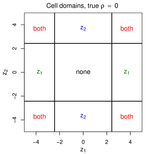
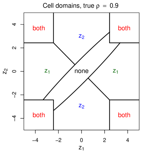
Figure 2: Bivariate domains where no cells are flagged, where only $z_{1}$ is flagged, where only $z_{2}$ is flagged, and where both are flagged, when the true correlation is $\rho=0$ (left panel) and when $\rho=0.9$ (right panel).

2.3 Simulation

To evaluate the performance of cellHandler we run a small simulation in which the uncontaminated data are $d$-variate Gaussian with $\bm{\mu}=\bm{0}$. Since cellwise methods are neither affine or orthogonal invariant, we consider underlying covariance matrices $\bm{\Sigma}$ of two types. Type ALYZ are the randomly generated correlation matrices of Agostinelli et al., (2015) which typically have relatively small correlations. Type A09 is given by $\Sigma_{jh}:=(-0.9)^{|j-h|}$ and contains both large and small correlations.

The outlying cells are generated as follows. The positions of the cells to be contaminated are obtained by randomly drawing $n\varepsilon$ indices in each column of the data matrix. Then we look at each row $(z_{1},\ldots,z_{d})$ with such cells, and denote the indices of those cells as the set $K=\{j(1),\ldots,j(k)\}$ of size $k$. Next, we replace $(z_{j(1)},\ldots,z_{j(k)})$ by the $k$-dimensional row $\bm{v}=\gamma\sqrt{k}\,\bm{u}^{\prime}/\operatorname{\mbox{MD}}(\bm{u},\bm{\mu}_{K},\bm{\Sigma}_{K})$ where $\bm{\mu}_{K}$ and $\bm{\Sigma}_{K}$ are restricted to the indices in $K$ and where $\bm{u}$ is the eigenvector of $\bm{\Sigma}_{K}$ with smallest eigenvalue. This procedures generates $\bm{v}$ which are structurally outlying in the subspace of the coordinates in $K$, while many of these cells will not be marginally outlying. This produces cellwise outliers that are more challenging than in the earlier literature, which used $\bm{v}=(\gamma,\ldots,\gamma)$.

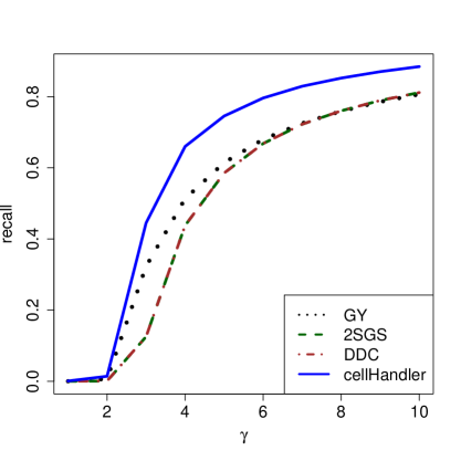
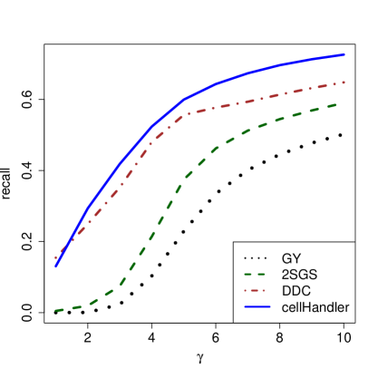
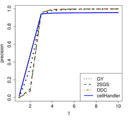
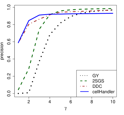
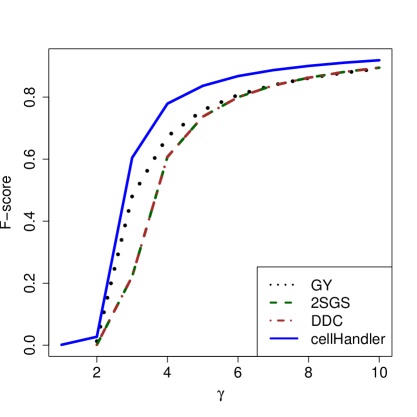
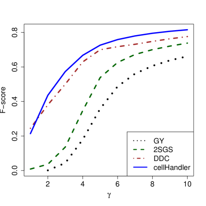
Figure 3: Comparison of methods for detecting cellwise outliers on data generated by the contaminated ALYZ model (left) and the contaminated A09 model (right), for $n=400$ points in $d=20$ dimensions. The plots show recall (top), precision (middle), and F-score (bottom).

Figure 3 shows the performance of cellHandler on samples of size $n=400$ in $d=20$ dimensions with $\varepsilon=20\%$ of cellwise outliers, using the covariance matrix estimated by the algorithm DDCW.DI described in Section 3.2. The other curves are from three existing techniques for flagging cells. The first one is the univariate Gervini-Yohai filter (GY) specified in (Agostinelli et al.,, 2015). The second is the multivariate DetectDeviatingCells (DDC) algorithm of Rousseeuw and Van den Bossche, (2018), available in the cellWise package (Raymaekers et al., , 2020) as the function DDC. The third is the default filter of the 2SGS method in (Leung et al., , 2017), which is a combination of a bivariate GY filter with DDC. The top panels in Figure 3 show the recall, which is the fraction of generated cellwise outliers that are flagged as such. The data in the left plot were generated by the contaminated ALYZ model, and on the right by the contaminated A09 model. We see that cellHandler has the highest recall at each $\gamma$. When $\gamma$ increases the cellwise outliers become marginally outlying, making them easier to flag. The middle row of the figure shows the precision, which is the fraction of cells flagged as outlying that were generated as such. We see that cellHandler does not have the best precision among competing methods at high $\gamma$, which is due to the tradeoff between precision and recall. Finally, the bottom row shows the F-score, also called the Dice coefficient (Dice, , 1945), which summarizes the performance of a binary classification through the harmonic mean of precision and recall. Based on this summary measure, cellHandler performs best.

3 Cellwise robust estimation of a covariance matrix

3.1 Existing approaches

The previous section described a method for flagging cellwise outliers when the true center $\bm{\mu}$ and covariance matrix $\bm{\Sigma}$ are known. Of course these are rarely known in practice, so they have to be estimated. The center $\bm{\mu}$ can be estimated quite easily by applying a robust estimator (like the median) to each coordinate. Estimating the covariance matrix $\bm{\Sigma}$ is the hard part. There exist several approaches to this problem.

A popular technique is to compute robust covariances between each pair of variables, and to assemble them in a matrix. To estimate these pairwise covariances, Öllerer and Croux, (2015) and Croux and Öllerer, (2016) use rank-based methods such as the Spearman and normal scores correlations. Tarr et al., (2016) instead propose to use the robust pairwise correlation estimator of Gnanadesikan and Kettenring, (1972) in combination with the robust scale estimator $Q_{n}$ of Rousseeuw and Croux, (1993). As the resulting matrix is not necessarily positive semidefinite (PSD), they then compute the nearest PSD matrix by the algorithm of Higham, (2002). All of these pairwise covariance estimators are fast to compute. We will compare the performance of these methods in Section 5.

A second approach is the snipEM procedure proposed by Farcomeni, (2014) and implemented in the R package snipEM of Farcomeni and Leung, (2019). Its first step flags cellwise outliers in each variable separately using a boxplot rule, and then ”snips” them, which means making them missing. The second step tries many interchanges that unsnip a randomly chosen snipped cell and at the same time snip a randomly chosen unsnipped cell, and only keeps an interchange when it increases the partial Gaussian likelihood. This procedure is slower than the pairwise covariance approach.

The current state of the art to deal with complex cellwise outliers is the two-step generalized S-estimator (2SGS) of Agostinelli et al., (2015) and Leung et al., (2017) implemented in the R package GSE (Leung et al., , 2019). In a first step, the method uses a filter (called 2SGS in Figure 3 above) to detect cellwise outliers. These cells are then set to missing, and the generalized S-estimator of Danilov et al., (2012) is run. A short survey of cellwise robust covariance estimators can be found in Sections 6.13 and 6.14 of Maronna et al., (2019).

3.2 The detection-imputation algorithm

Our algorithm for constructing a cellwise robust covariance matrix starts by standardizing the columns of the dataset as in the beginning of Section 2.1. Next, we compute initial estimators $\bm{\hat{\mu}}^{0}$ and $\bm{\widehat{\Sigma}}^{0}$. For this we can use the 2SGS estimator of Leung et al., (2017) described above. We will also try a different initial estimator called DDCW, which is a combination of the DDC method (Rousseeuw and Van den Bossche, , 2018) and the wrapped covariance matrix of Raymaekers and Rousseeuw, (2019). This initial estimator is described in Section D of the Appendix.

The detection-imputation (DI) algorithm then alternates the D-step and the I-step, both described below.

D-step: detecting outlying cells across all rows.
The D-step first applies the cellHandler method of Section 2 to each row $\bm{z}_{i}^{\prime}$ based on the estimates $\bm{\hat{\mu}}^{t-1}$ and $\bm{\widehat{\Sigma}}^{t-1}$ from the previous iteration step. This way each row $\bm{z}_{i}^{\prime}$ gets a ranking of its cells $z_{ij}$ . From the $\Delta_{k}$ in its path we construct a nonincreasing sequence of criterion values $C_{ij}\coloneqq\max_{h\geqslant k(j)}\Delta_{h}$ . If any cells $z_{ih}$ are missing (NA) these are put in front of the path with $C_{ih}\coloneqq+\infty$.

Should some columns have too many flagged cells (including NA’s) it could become difficult to estimate a correlation between them, especially if the flagged sets overlap little. Even worse, flagging all cells in a column would remove all information about that variable. Therefore, we impose a maximal number of flagged cells in each column, including the NA’s. This number is $n\,\mbox{{maxCol}}$ where the input parameter maxCol is set to $25\%$ by default. Note that this is a constraint on the columns, whereas we are flagging cells by row. We resolve this with the following algorithm:

- sort the criterion values $C_{ij}$ of all cells in the matrix in decreasing order;

- walk down this list. If a $C_{ij}$ lies below the cutoff value $q$ we “lock” row $i$, i.e. no cells of row $i$ can be flagged any more. If $C_{ij}>q$ the cell is flagged, unless it belongs to a column which already has $\,n\,\mbox{{maxCol}}\,$ flagged cells. In the latter case, row $i$ is locked also.

This procedure yields a (possibly empty) list of flagged cells in each row, which overall contains the most outlying cells subject to the maxCol constraint.

I-step: Re-estimate $\mu$ and $\bm{\Sigma}$ .
The I-step is basically one step of the EM algorithm which considers the flagged cells as missing. However, it is computationally more efficient since it reuses results that are already available. In each row, the set of flagged cells is one of the active sets considered by LAR in cellHandler, so its coefficient $\bm{\hat{\theta}}_{1}$ from Proposition 2 is known. This makes it trivial to impute the flagged cells, so the E-step of EM requires no additional computation. Next, $\bm{\hat{\mu}}^{t}$ and $\bm{\widehat{\Sigma}}^{t}$ are computed as in the M-step, as described in more detail in Section E of the Appendix. This iterative procedure stops when both $\bm{\hat{\mu}}^{t}-\bm{\hat{\mu}}^{t-1}$ and $\bm{\widehat{\Sigma}}^{t}-\bm{\widehat{\Sigma}}^{t-1}$ are small. At the end of the DI algorithm we unstandardize $\bm{\hat{\mu}}$ and $\bm{\widehat{\Sigma}}$ using the univariate location and scale estimates of the original data columns.

The time complexity of the DI algorithm is $O(Tnd^{3})$ where $T$ is the number of iteration steps. This is the same complexity as that of the classical EM algorithm for covariance estimation with missing data.

Note that for the DI method to work, the initial covariance matrix (whether 2SGS or DDCW) and those in all iteration steps need to be invertible. This requires that $n>d$, so for now the approach does not allow for $d\geqslant n$. Possible extensions are a topic for further research, and would likely require penalization or other forms of regularization.

4 Measuring scatter matrix discrepancy

In the simulation in the next section we want to measure how much an estimated scatter matrix deviates from the true underlying positive definite (PD) scatter matrix. For this we need a discrepancy measure for scatter matrices. Here we will construct a pre-existing discrepancy measure from first principles, in order to dispel a common misconception that this measure would only make sense when the underlying data follow a multivariate normal (Gaussian) distribution.

Suppose we want to measure how much a scatter matrix $\bm{A}$ deviates from a reference scatter matrix $\bm{B}$, where the $d\times d$ matrix $\bm{B}$ is PD but $\bm{A}$ only needs to be positive semidefinite (PSD). A simple measure of this type is

$$||\bm{A}-\bm{B}||_{2}=\Big{(}\sum_{i=1}^{d}\sum_{j=1}^{d}\,(a_{ij}-b_{ij})^{2}\,\Big{)}^{1/2}$$ (4)

but it is insufficiently suited to our scatter matrix context, as it does not tell us whether $\bm{A}$ is singular. And this is important, since a singular scatter matrix $\bm{A}$ cannot be used as an approximation of $\bm{B}$, for instance when computing a Mahalanobis-style statistical distance as in (2.1) which requires the inverse matrix.

In order to stay in the land of scatter matrices we instead compute

$$\bm{C}=\bm{B}^{-1/2}\bm{A}\,\bm{B}^{-1/2}\;.$$

(The matrix $\bm{C}$ can be seen as the scatter $\bm{A}$ in the coordinate system where $\bm{B}$ is sphered/whitened, since $\bm{B}^{-1/2}\bm{B}\,\bm{B}^{-1/2}=\bm{I}$.) Note that $\bm{A}=\bm{B}$ if and only if $\bm{C}=\bm{I}$, so we want to measure how far $\bm{C}$ is from $\bm{I}$ in a way that is relevant for scatter matrices. Since the matrix $\bm{C}$ is PSD its eigenvalues are nonnegative, so we can denote them as $\eta_{1}\geqslant\ldots\geqslant\eta_{d}\geqslant 0$. We want the discrepancy measure to be zero if all $\eta_{j}=1$, to go to $+\infty$ when $\bm{C}$ explodes in the sense that $\eta_{1}\rightarrow+\infty$, and also when $\bm{C}$ implodes, i.e. $\eta_{d}\rightarrow 0$. Concentrating on a single eigenvalue $\eta$ we want a continuous function $h(\eta)$ on all $\eta\geqslant 0$ with the properties $h(\eta)\geqslant 0$, $h(1)=0$, and $h(\eta)\rightarrow+\infty$ when $\eta\rightarrow+\infty$ or $\eta\rightarrow 0$. Many such functions can be constructed. One of them is $h(\eta)=\eta-1-\log(\eta)$. Note that $h(\eta)\geqslant 0$ since $\log(\eta)$ is concave and $\eta-1$ is its tangent line at $\eta=1$. The function $h$ decreases on $[0,1[$, reaches its minimum in 1 with $h(1)=0$, and increases on $]1,+\infty[$. Therefore it makes sense to define the discrepancy of $\bm{A}$ relative to $\bm{B}$ as

$$D(\bm{A},\bm{B}):=\sum_{j=1}^{d}h(\eta_{j})=\sum_{j=1}^{d}(\eta_{j}-1-\log(\eta_{j}))$$ (5)

which is nonnegative since each term is. Note that $\bm{A}=\bm{B}$ is equivalent to $D(\bm{A},\bm{B})=0$, and that a singular $\bm{A}$ attains $D(\bm{A},\bm{B})=+\infty$.

The entire construction of $D(\bm{A},\bm{B})$ above only uses the PSD property of scatter matrices, and is not at all restricted to multivariate normally distributed data. That confusion is due to the following property:

Proposition 4.

In the special case where $\bm{X}$ and $\bm{Y}$ are $d$-variate random vectors distributed as $\bm{X}\sim N(\bm{0},\bm{A})$ and $\bm{Y}\sim N(\bm{0},\bm{B})$ in which both $\bm{A}$ and $\bm{B}$ are PD, the discrepancy $D(\bm{A},\bm{B})$ coincides with the Kullback-Leibler divergence $\operatorname{\mbox{KL}}(\bm{X},\bm{Y})$.

The proof is in Section F of the Appendix. Note that when both $\bm{A}$ and $\bm{B}$ are PD also $D(\bm{B},\bm{A})$ exists, but it does not equal $D(\bm{A},\bm{B})$. Instead we obtain, along the same lines, $D(\bm{B},\bm{A})=\sum_{j=1}^{d}h(1/\eta_{j})$. However, it is possible to symmetrize the discrepancy $D(.,.)$ by replacing the $h$ in (5) by a function $\tilde{h}$ for which $\tilde{h}(1/\eta)=\tilde{h}(\eta)$ for all $\eta>0$, such as $\tilde{h}(\eta)=\eta+1/\eta-2$. One could also use the function $\tilde{h}(\eta)=|\log(\eta)|$ so $D(\bm{A},\bm{B})$ becomes the $L^{1}$ norm of $(\log(\eta_{1}),\ldots,\log(\eta_{d}))$.

5 Simulation results

We simulate the estimators of covariance matrices discussed in the previous section. The data is generated as in Subsection 2.3, with dimensions $d=10$, $20$ and $40$. The fraction of contaminated cells is $\varepsilon=0.1,0.2$ in which $\gamma$ varies from $1$ to $10$. In each replication we compute the discrepancy (5) of the estimate $\widehat{\bm{\Sigma}}$ from the underlying $\bm{\Sigma}$, and then average the discrepancy over all replications. We show the results for $\varepsilon=0.2$, since this is the most challenging scenario. The results for $\varepsilon=0.1$ were qualitatively similar.

Figure 4 compares the proposed methods to the existing approaches described in Subsection 3.1, for $d=10$. Since $\varepsilon=0.2$ there are on average two cellwise outliers per row. Gaussian rank (Grank) and Spearman refer to the covariance matrices of Öllerer and Croux, (2015) and Croux and Öllerer, (2016) using those rank correlations. The Gnanadesikan-Kettenring procedure of Tarr et al., (2016) is labeled GKnpd. Next, the snipEM method of Farcomeni, (2014) and the 2SGS estimator of Leung et al., (2017) are plotted. The method 2SGS.DI uses 2SGS as initial estimator followed by the new DI method of Section 3.2. Also the initial estimator DDCW described in Section D of the Appendix is shown, as well as DI applied to it.

ALYZ model, 20% outliers, $\bm{d=10}$

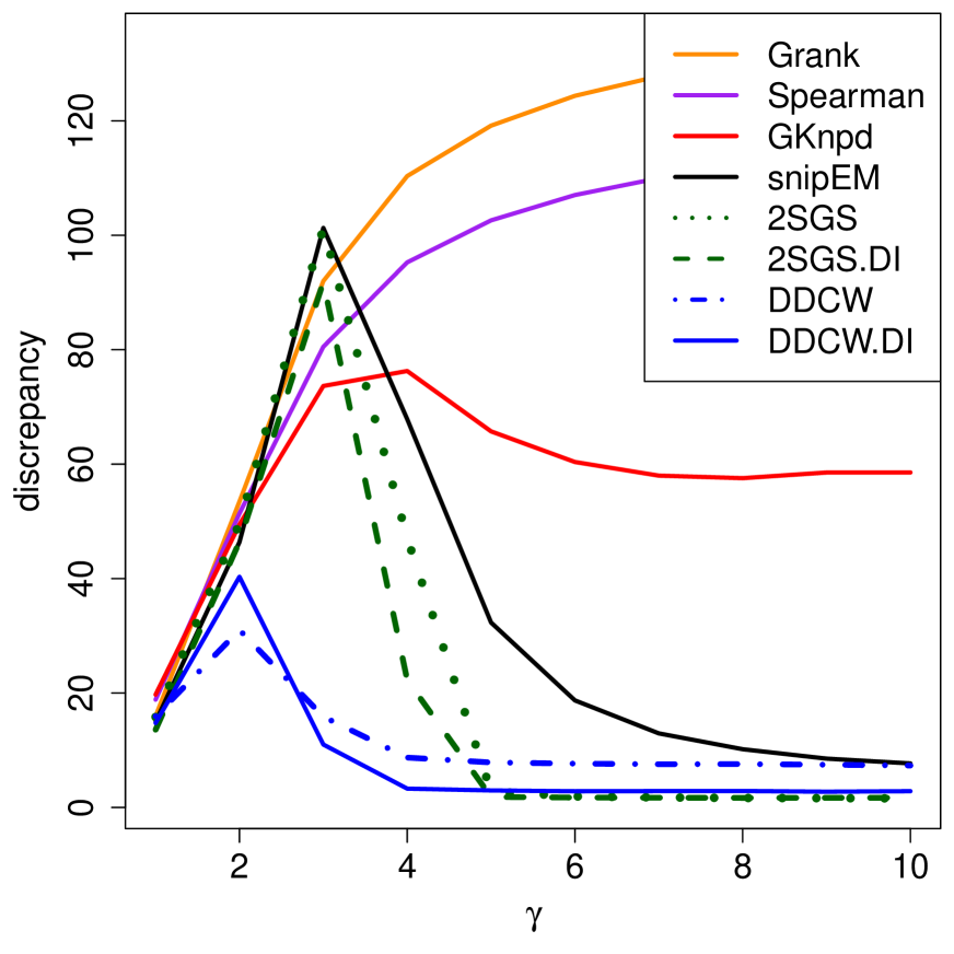
A09 model, 20% outliers, $\bm{d=10}$

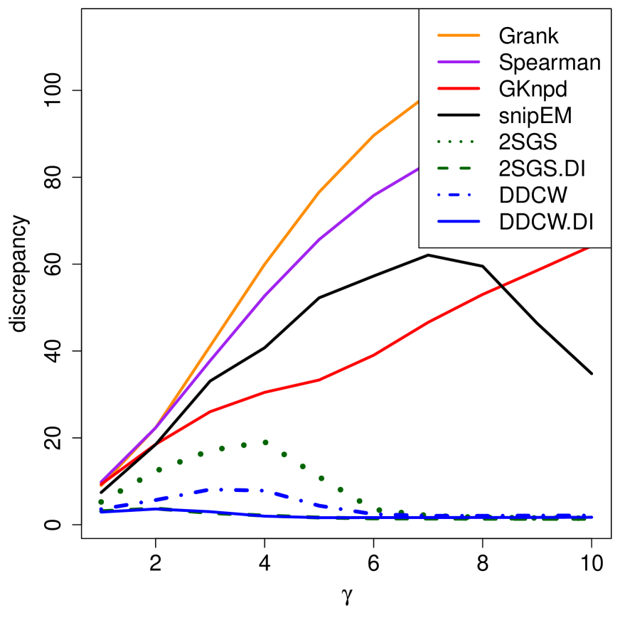
Figure 4: Discrepancy $D(\widehat{\bm{\Sigma}},\bm{\Sigma})$ of estimated covariance matrices for $d=10$, $n=100$.

We see that the three pairwise methods Grank, Spearman and GKnpd pay for their fast computation by a high discrepancy. The snipEM method does better for high $\gamma$, in part because the boxplot rule in its first step snips marginally outlying cells. The three pairwise methods do not use such a rule to flag marginally outlying cells, so high $\gamma$ values impact them more. The state of the art method 2SGS does substantially better, and is improved by applying DI to it, both in the ALYZ and A09 models. The same holds for DDCW and DDCW.DI. Note that DI improves the results more under A09 than ALYZ, because A09 has bigger correlations so DI has more opportunities to make a difference.

We now consider higher dimensions, starting with $d=20$ in the top panels of Figure 5. The curves of Grank, Spearman, GKnpd and snipEM were much higher in this case, so we only show the four best performing methods in order to see the differences between them. Also here the DI algorithm substantially improves upon the initial estimators. The improvement is largest under A09 which contains some high correlations. For $d=40$ (bottom panels) we see similar patterns.

ALYZ model, 20% outliers, $\bm{d=20}$

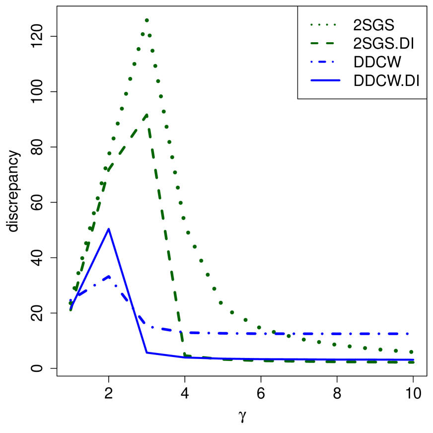
A09 model, 20% outliers, $\bm{d=20}$

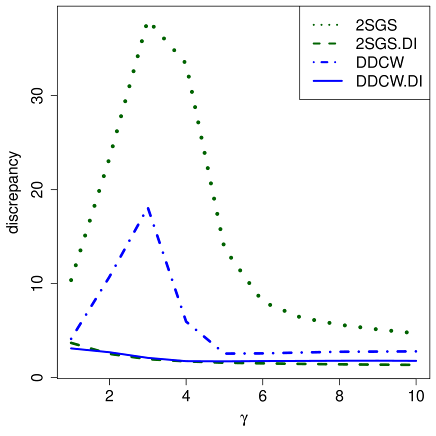
ALYZ model, 20% outliers, $\bm{d=40}$

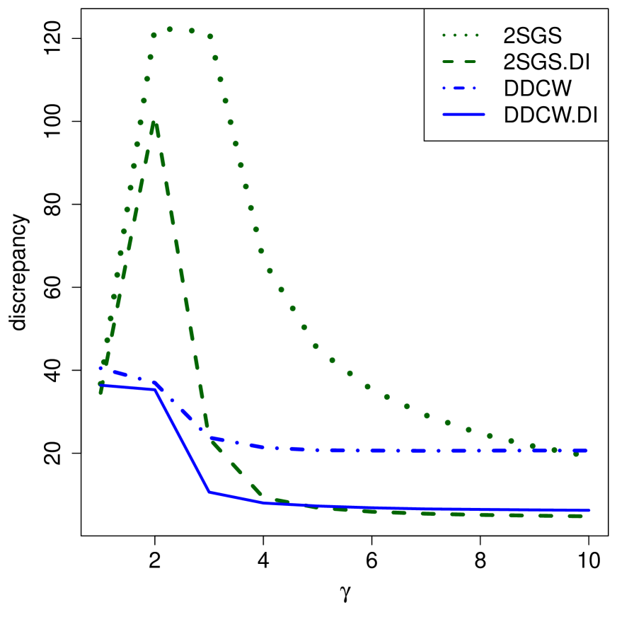
A09 model, 20% outliers, $\bm{d=40}$

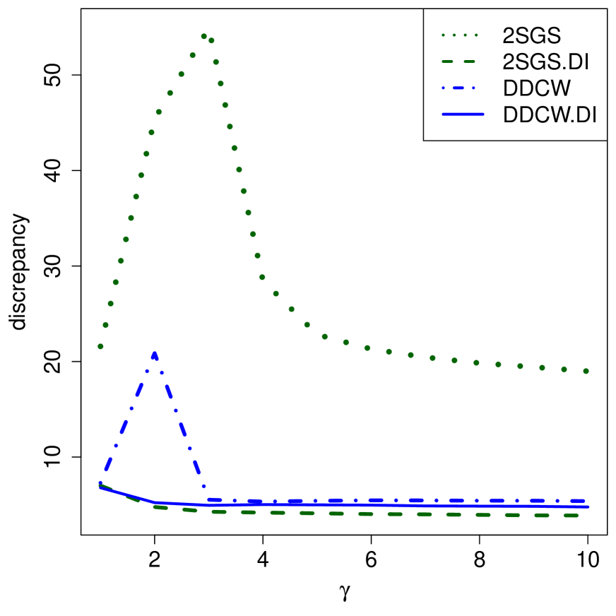
Figure 5: Discrepancy $D(\widehat{\bm{\Sigma}},\bm{\Sigma})$ given by (5) of estimated covariance matrices for $d=20$ and $n=400$ (top panels) and for $d=40$ and $n=800$ (bottom panels).

Section I of the Appendix shows the results of a simulation in which the data are contaminated by $10\%$ of cellwise outliers generated as above, plus $10\%$ of rowwise outliers. In this particular setting ”rowwise outliers” refers to rows in which all cells are contaminated in the same way as before, that is, rows with $d$ cellwise outliers. The initial estimators 2SGS and DDCW attempt to downweight or discard such rows. The results are qualitatively similar to those in Figures 4 and 5.

6 Example: volatile organic compounds in children

We study a dataset of volatile organic compounds (VOCs) in human urinary samples. The data was taken from the publicly available website of the National Health and Nutrition Examination Survey (NHANES, , 2019), using the most recent available epoch. Such VOC metabolites are commonly monitored since chronic exposure to high levels of some VOCs can lead to a number of health problems such as cancer and neurocognitive dysfunction. The original dataset consists of 29 VOC metabolites, but we focus on a subset of 16 variables obtained by removing columns with a lot of missing values and/or zero median absolute deviation. Section J in the Appendix contains a table with the VOCs analyzed. In order to obtain a relatively homogeneous subset, we selected the data for children aged 10 or younger. The final dataset contained 512 subjects. We log-transformed the concentrations to make the variables roughly Gaussian (apart from possible outliers).

We estimated the covariance matrix of the data by the DI algorithm, starting from the DDCW initial estimator. The algorithm converged after 7 steps. Using the resulting covariance estimate we ran the cellHandler algorithm with cutoff $\sqrt{\chi^{2}_{1,0.99}}\approx 2.57$ to detect outlying cells. The corresponding cellmap of the first 20 children in the list was shown as Figure 1 in the introduction. Each row of the cellmap corresponds to a child, with inlying cells colored yellow. Red colored cells indicate that their value is higher than predicted given the inlying cells of that row, while blue cells indicate lower than predicted values. The more extreme the residual, the more intense the color.

One variable that stood out was URXCYM (N-Acetyl-S-(2-cyanoethyl)-L-cysteine) in which cellHandler indicated $11\%$ of large cell residuals. This was particularly striking since that variable had fewer than $2\%$ of marginal outliers using the same cutoff $\sqrt{\chi^{2}_{1,0.99}}$ on the absolute standardized values, and these were rather nearby (note that even for perfectly Gaussian data there would already be $1\%$ of absolute standardized values above this cutoff). Figure 6 plots the cell residuals (which are zero for cells that were not flagged) versus the robustly standardized marginal values, with the cutoffs indicated by horizontal and vertical lines. Most of the outlying cellwise residuals correspond to inlying marginal values. These children have extreme URXCYM values relative to their other VOCs.

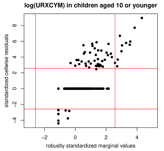
Figure 6: Plot of standardized cell residuals of log(URXCYM) obtained by cellHandler, versus the robustly standardized values of log(URXCYM) on its own.

Interestingly, URXCYM is a well known biomarker for identifying smokers among adults, see e.g. Chen et al., (2019), since it typically results from the metabolization of acrylonitrile, a volatile liquid present in tobacco smoke. But in this example we are studying children, who are not supposed to smoke. In search of an explanation we combined the VOC data with the questionnaire data available on the same website (NHANES, , 2019). Among many other things, these data contain information on the smoking status of the adults (usually parents) in the same household. These fell into four categories: only nonsmoking adults, smoking adults who do not smoke inside the home, one adult smoking in the home, and two adults smoking in the home. The blue curve in Figure 7 shows the percentage of children with URXCYM cell residuals above the cutoff, in each of these categories. They go from 4.7% in households with only nonsmoking adults up to 72.7% in homes where two adults smoke, indicating that passive smoking has a measurable effect on children. On the other hand, if we were to look only at the marginal URXCYM values (red curve) no such effect is visible.

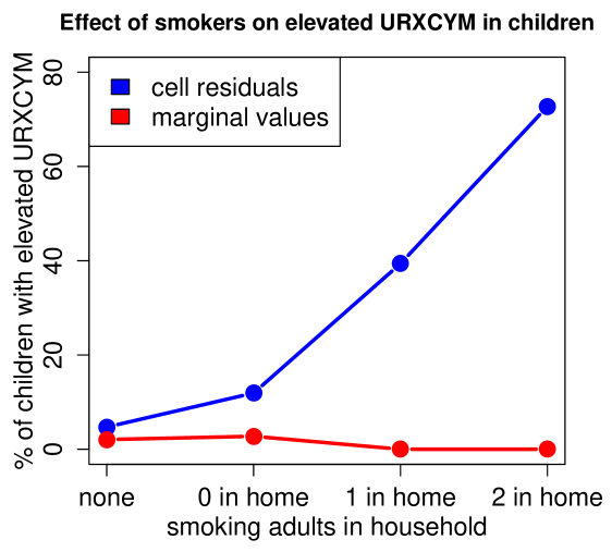
Figure 7: The blue curve shows the percentage of elevated URXCYM cell residuals in function of the smoking status of adult family members. The red curve shows the percentage of elevated marginal URCYM values.

The example shows that the effect of exposing children to tobacco smoke could be underestimated when only performing univariate analyses on biomarkers. This illustrates that cell residuals obtained by cellHandler may add valuable information to a dataset.

7 Conclusion

The proposed cellHandler method is the first to detect cellwise outliers based on robust estimates of location and covariance. It is also a major component of the detection-imputation (DI) algorithm that computes such cellwise robust estimates. Note that both methods can deal with missing values in the data, since these are imputed along the way.

The performance of cellHandler and DI was illustrated by simulation. A real example illustrated that the common medical practice of comparing individual biomarkers to their tolerance limits can benefit from the use of cellwise residuals.

Acknowledgment. This research was funded by projects of Internal Funds KU Leuven.

Software Availability. The methods proposed here are available as the functionscellHandler and DI in the R package cellWise (Raymaekers et al., , 2020) on CRAN.
It also contains a vignette which reproduces the example in Section 6.

Appendix A Proof of Proposition 2

Proof.

We first split up the relevant matrices in blocks. Denote

$$\bm{\Sigma}^{-1}=\begin{bmatrix}\bm{\Sigma}_{11}^{*}&\bm{\Sigma}_{12}^{*}\\ \bm{\Sigma}_{21}^{*}&\bm{\Sigma}_{22}^{*}\end{bmatrix}\quad\quad\mbox{ and }\quad\quad\bm{\Sigma}^{-1/2}=\begin{bmatrix}\bm{\tilde{\Sigma}}_{11}&\bm{\tilde{\Sigma}}_{12}\\ \bm{\tilde{\Sigma}}_{21}&\bm{\tilde{\Sigma}}_{22}\end{bmatrix}\;\;.$$

Let the $k$-variate $\bm{\hat{\theta}}$ be the solution to the ordinary least squares regression problem

$$\operatorname{\mbox{argmin}}_{\bm{\theta}}||\bm{\Sigma}^{-1/2}(\bm{z}-\bm{\mu})-(\bm{\Sigma}^{-1/2})_{\bm{\cdot}1}\bm{\theta}||_{2}^{2}$$

where $(\bm{\Sigma}^{-1/2})_{\bm{\cdot}1}$ denotes the first $k$ columns of the matrix $\bm{\Sigma}^{-1/2}$.
Then we know that

$$\bm{\hat{\theta}} =\left(\begin{bmatrix}\bm{\tilde{\Sigma}}_{11}\\ \bm{\tilde{\Sigma}}_{21}\end{bmatrix}^{\prime}\,\begin{bmatrix}\bm{\tilde{\Sigma}}_{11}\\ \bm{\tilde{\Sigma}}_{21}\end{bmatrix}\right)^{-1}\begin{bmatrix}\bm{\tilde{\Sigma}}_{11}\\ \bm{\tilde{\Sigma}}_{21}\end{bmatrix}^{\prime}\,\bm{\Sigma}^{-1/2}(\bm{z}-\bm{\mu})$$

$$=(\bm{\Sigma}_{11}^{*})^{-1}\begin{bmatrix}\bm{\tilde{\Sigma}}_{11}\\ \bm{\tilde{\Sigma}}_{21}\end{bmatrix}^{\prime}\,\bm{\Sigma}^{-1/2}(\bm{z}-\bm{\mu}).$$

Now observe that

$$\bm{z}_{1}-\bm{\hat{\theta}} =\bm{z}_{1}-(\bm{\Sigma}_{11}^{*})^{-1}\begin{bmatrix}\bm{\tilde{\Sigma}}_{11}\\ \bm{\tilde{\Sigma}}_{21}\end{bmatrix}^{\prime}\,\bm{\Sigma}^{-1/2}(\bm{z}-\bm{\mu})$$

$$=\bm{z}_{1}-(\bm{\Sigma}_{11}^{*})^{-1}[\bm{\Sigma}_{11}^{*}\;\bm{\Sigma}_{12}^{*}][\bm{z}_{1}-\bm{\mu}_{1}\;\;\bm{z}_{2}-\bm{\mu}_{2}]$$

$$=\bm{z}_{1}-[I_{k}\;\;(\bm{\Sigma}_{11}^{*})^{-1}\bm{\Sigma}_{12}^{*}][\bm{z}_{1}-\bm{\mu}_{1}\;\;\bm{z}_{2}-\bm{\mu}_{2}]$$

$$=\bm{z}_{1}-(\bm{z}_{1}-\bm{\mu}_{1})-(\bm{\Sigma}_{11}^{*})^{-1}\bm{\Sigma}_{12}^{*}(z_{2}-\bm{\mu}_{2})$$

$$=\bm{\mu}_{1}+\bm{\Sigma}_{12}\bm{\Sigma}_{22}^{-1}(\bm{z}_{2}-\bm{\mu}_{2})$$

where the last equality follows from $-(\bm{\Sigma}_{11}^{*})^{-1}\bm{\Sigma}_{12}^{*}=\bm{\Sigma}_{12}\bm{\Sigma}_{22}^{-1}$ iff $-\bm{\Sigma}_{12}^{*}\bm{\Sigma}_{22}=\bm{\Sigma}_{11}^{*}\bm{\Sigma}_{12}$ iff $[\bm{\Sigma}_{11}^{*}\;\bm{\Sigma}_{12}^{*}][\bm{\Sigma}_{12}\bm{\Sigma}_{22}]^{\prime}\,=0$ which follows from $\bm{\Sigma}^{-1}\bm{\Sigma}=I$. ∎

Appendix B Proof of Proposition 3

Proof.

We will use the notation $\bm{\hat{\theta}}_{1}=\operatorname{\mbox{argmin}}_{\bm{\theta}_{1}}||\bm{\Sigma}^{-1/2}(\bm{z}-\bm{\mu})-(\bm{\Sigma}^{-1/2})_{\bm{\cdot}1}\bm{\theta}_{1}||_{2}^{2}$ for the OLS fit, and $\mbox{RSS}_{k}=||\bm{\Sigma}^{-1/2}(\bm{z}-\bm{\mu})-(\bm{\Sigma}^{-1/2})_{\bm{\cdot}1}\bm{\hat{\theta}}_{1}||_{2}^{2}$.

Part 1.
For $k=d$ we know from (2.1) that $\mbox{RSS}_{d}=0$. Now let $1\leqslant k\leqslant d-1$. We want to show that $\mbox{RSS}_{k}=(\bm{z}_{2}-\bm{\mu}_{2})^{\prime}\,\bm{\Sigma}_{22}^{-1}(\bm{z}_{2}-\bm{\mu}_{2})$. Let $\bm{\hat{\theta}}\coloneqq[\bm{\hat{\theta}}_{1}^{\prime}\,\;0\;\ldots\;0]^{\prime}$ be the $d$-variate vector with coefficients $\bm{\hat{\theta}}_{1}$ followed by $d-k$ zeroes.

We now have that

$$\mbox{RSS}_{k} =||\bm{\Sigma}^{-1/2}(\bm{z}-\bm{\mu})-(\bm{\Sigma}^{-1/2})_{\bm{\cdot}1}\bm{\hat{\theta}}_{1}||_{2}^{2}$$

$$=||\bm{\Sigma}^{-1/2}(\bm{z}-\bm{\mu})-\bm{\Sigma}^{-1/2}\bm{\hat{\theta}}||_{2}^{2}$$

$$=(\bm{z}-\bm{\mu}-\bm{\hat{\theta}})^{\prime}\,\bm{\Sigma}^{-1}(\bm{z}-\bm{\mu}-\bm{\hat{\theta}})$$

$$=[\bm{z}_{1}-\bm{\mu}_{1}-\bm{\hat{\theta}}_{1}\;\;\;\bm{z}_{2}-\bm{\mu}_{2}]^{\prime}\,\bm{\Sigma}^{-1}\,[\bm{z}_{1}-\bm{\mu}_{1}-\bm{\hat{\theta}}_{1}\;\;\;\bm{z}_{2}-\bm{\mu}_{2}]\;\;.$$

Following page 47 of Petersen and Pedersen, (2012) we can write $\bm{\Sigma}^{-1}=\bm{A}\bm{B}\bm{A}^{\prime}\,$ with

$$\bm{A}\coloneqq\begin{bmatrix}\bm{I}&\bm{0}\\ -\bm{\Sigma}_{22}^{-1}\bm{\Sigma}_{21}&\bm{I}\end{bmatrix}\quad\quad\mbox{ and }\quad\quad\bm{B}\coloneqq\begin{bmatrix}\bm{C}_{1}^{-1}&\bm{0}\\ \bm{0}&\bm{\Sigma}_{22}^{-1}\end{bmatrix}$$

where $\bm{C}_{1}\coloneqq\bm{\Sigma}_{11}-\bm{\Sigma}_{12}\bm{\Sigma}_{22}^{-1}\bm{\Sigma}_{21}$ . We now have that

$$[\bm{z}_{1}-\bm{\mu}_{1}-\bm{\hat{\theta}}_{1}\;\;\;\bm{z}_{2}-\bm{\mu}_{2}]^{\prime}\,\bm{A} =[\bm{z}_{1}-\bm{\mu}_{1}-\bm{\hat{\theta}}_{1}-(\bm{z}_{2}-\bm{\mu}_{2})\bm{\Sigma}_{22}^{-1}\bm{\Sigma}_{21}\;\;\;\bm{z}_{2}-\bm{\mu}_{2}]^{\prime}$$

$$=[\bm{0}\;\;\;\bm{z}_{2}-\bm{\mu}_{2}]^{\prime}$$

using the result of Proposition 2. Therefore,

$$\mbox{RSS}_{k} =[\bm{z}_{1}-\bm{\mu}_{1}-\bm{\hat{\theta}}_{1}\;\;\;\bm{z}_{2}-\bm{\mu}_{2}]^{\prime}\,\bm{\Sigma}^{-1}\,[\bm{z}_{1}-\bm{\mu}_{1}-\bm{\hat{\theta}}_{1}\;\;\;\bm{z}_{2}-\bm{\mu}_{2}]$$

$$=[\bm{0}\;\;\;\bm{z}_{2}-\bm{\mu}_{2}]^{\prime}\,\bm{B}\,[\bm{0}\;\;\;\bm{z}_{2}-\bm{\mu}_{2}]$$

$$=(\bm{z}_{2}-\bm{\mu}_{2})^{\prime}\,\bm{\Sigma}_{22}^{-1}\,(\bm{z}_{2}-\bm{\mu}_{2})\;\;.$$

Part 2.
We will now show that the differences in RSS follow a $\chi^{2}(1)$ distribution, that is$\Delta_{k}\coloneqq\mbox{RSS}_{k-1}-\mbox{RSS}_{k}\sim\chi^{2}(1)$ assuming that $\bm{z}=[\bm{z}_{1}^{\prime}\;\bm{z}_{2}^{\prime}]^{\prime}$ is multivariate Gaussian with mean $\bm{\mu}$ and covariance matrix $\bm{\Sigma}$. For $k=0$ we set by convention $\bm{\hat{\theta}}\coloneqq\bm{0}$ and $\mbox{RSS}_{0}\coloneqq||\bm{\Sigma}^{-1/2}(\bm{z}-\bm{\mu})||_{2}^{2}$.

We show the result for $k=1$ as the subsequent steps are analogous. The reasoning below is similar to Appendix A.2 of Danilov, (2010) where the cells were not yet ranked from most to least outlying. As in Part 1 of the proof we can write $\bm{\Sigma}^{-1}=\bm{A}\bm{B}\bm{A}^{\prime}\,$ with

$$\bm{A}=\begin{bmatrix}1&\bm{0}\\ -\bm{\Sigma}_{22}^{-1}\bm{\Sigma}_{21}&\bm{I}\end{bmatrix}\quad\quad\mbox{ and }\quad\quad\bm{B}=\begin{bmatrix}C_{1}^{-1}&\bm{0}\\ \bm{0}&\bm{\Sigma}_{22}^{-1}\end{bmatrix}$$

where this time $C_{1}=\bm{\Sigma}_{11}-\bm{\Sigma}_{12}\bm{\Sigma}_{22}^{-1}\bm{\Sigma}_{21}$ is a scalar. We can then write

$$\mbox{RSS}_{0} =(\bm{z}-\bm{\mu})^{\prime}\,\bm{\Sigma}^{-1}(\bm{z}-\bm{\mu})$$

$$=(\bm{z}-\bm{\mu})^{\prime}\,\bm{A}\bm{B}\bm{A}^{\prime}\,(\bm{z}-\bm{\mu})$$

$$=[z_{1}-\mu_{1}-(\bm{z}_{2}-\bm{\mu}_{2})\bm{\Sigma}_{22}^{-1}\bm{\Sigma}_{21}\;\;\;\bm{z}_{2}-\bm{\mu}_{2}]^{\prime}\,\bm{B}\,[z_{1}-\mu_{1}-(\bm{z}_{2}-\bm{\mu}_{2})\bm{\Sigma}_{22}^{-1}\bm{\Sigma}_{21}\;\;\;\bm{z}_{2}-\bm{\mu}_{2}]$$

$$=\left((z_{1}-\mu_{1}^{*})/\sigma_{1}^{*}\right)^{2}+(\bm{z}_{2}-\bm{\mu}_{2})^{\prime}\,\bm{\Sigma}_{22}^{-1}(\bm{z}_{2}-\bm{\mu}_{2})$$

$$=((z_{1}-\mu_{1}^{*})/\sigma_{1}^{*})^{2}+\mbox{RSS}_{1}$$

where $\mu_{1}^{*}\coloneqq\mu_{1}+(\bm{z}_{2}-\bm{\mu}_{2})\bm{\Sigma}_{22}^{-1}\bm{\Sigma}_{21}$ and $\sigma_{1}^{*}\coloneqq\sqrt{C_{1}}$. So we obtain

$$\Delta_{1}=\mbox{RSS}_{0}-\mbox{RSS}_{1}=((z_{1}-\mu_{1}^{*})/\sigma_{1}^{*})^{2}$$

and this is the square of a standard Gaussian variable since $z_{1}-\mu_{1}^{*}$ is Gaussian with expectation 0 and standard deviation $\sigma_{1}^{*}$ . We thus have $\Delta_{1}\sim\chi^{2}(1)$. ∎

Appendix C Implementation of the cellHandler algorithm

The LAR component of cellHandler is a regression of $\bm{\tilde{Y}}$ on $\bm{\dot{X}}$ as defined in the paper. Since this regression has no intercept and we need to preserve the column scaling in $\bm{\dot{X}}$, we run the function lars::lar with the options intercept=F and normalize=F.

For the imputations in Proposition 2 and the RSS in Proposition 3 we require the OLS fits $\,\bm{\hat{\theta}}_{A}\,$ minimizing $\;||\bm{\Sigma}^{-1/2}(\bm{z}-\bm{\mu})-(\bm{\Sigma}^{-1/2})_{A}\,\bm{\theta}_{1}||_{2}^{2}\;$ where $A$ is the set of active predictor variables in every step of LAR. Fortunately, these can be obtained without significant additional computation time because each step of LAR already carries out the QR decomposition of $\,(\bm{\dot{X}}_{A})^{\prime}\,\bm{\dot{X}}_{A}\,$ where $\bm{\dot{X}}_{A}$ is the submatrix of $\bm{\dot{X}}$ consisting of the columns in $A$. The resulting OLS regression vectors $\,\bm{\hat{\beta}}_{A}\,$ obtained by LAR (which contain zeroes for the inactive variables) are then easily rescaled to $\,\bm{\hat{\theta}}_{A}=\bm{W}^{-1}\bm{\hat{\beta}}_{A}$ .

Appendix D Description of the initial estimator DDCW

The Detection-Imputation (DI) method of Section 3.2 needs initial cellwise robust estimates $\bm{\hat{\mu}}^{0}$ and $\bm{\widehat{\Sigma}}^{0}$ of location and covariance. One option is to insert the 2SGS estimator of Leung et al., (2017). We also developed a different initial estimator called DDCW, which we describe here. Its steps are:

1. Drop variables with too many missing values or zero median absolute deviation, and continue with the remaining columns.

2. Run the DetectDeviatingCells (DDC) method (Rousseeuw and Van den Bossche, , 2018) with the constraint that no more than $n\,maxCol$ cells are flagged in any variable. DDC also rescales the variables, and may delete some cases. Continue with the remaining imputed and rescaled cases denoted as $\bm{z}_{i}$ .

3. Project the $\bm{z}_{i}$ on the axes of their principal components, yielding the transformed data points $\bm{\tilde{z}}_{i}$ .

4. Compute the wrapped location $\bm{\hat{\mu}}_{w}$ and covariance matrix $\bm{\widehat{\Sigma}}_{w}$ (Raymaekers and Rousseeuw, , 2019) of these $\bm{\tilde{z}}_{i}$ . Next, compute the temporary points $\bm{u}_{i}=(u_{i1},...,u_{id})$ given by $u_{ij}=\max\{\min\{\tilde{z}_{ij}-(\bm{\hat{\mu}}_{w})_{j},2\},-2\}$. Then remove all cases for which the squared robust distance $\operatorname{\mbox{RD}}^{2}(i)=\bm{u}_{i}^{\prime}\bm{\widehat{\Sigma}}_{w}^{-1}\bm{u}_{i}$ exceeds $\chi^{2}_{d,q}\operatorname{\mbox{median}}_{h}(\operatorname{\mbox{RD}}^{2}(h))/\chi^{2}_{d,0.5}$ .

5. Project the remaining $\bm{\tilde{z}}_{i}$ on the eigenvectors of $\bm{\widehat{\Sigma}}_{w}$ and again compute a wrapped location and covariance matrix.

6. Transform these estimates back to the original coordinate system of the imputed data, and undo the scaling. This yields the estimates $\bm{\hat{\mu}}^{0}$ and $\bm{\widehat{\Sigma}}^{0}$ .

Note that DDCW can handle missing values since the DDC method in step 2 imputes them. The reason for the truncation in the rejection rule in step 4 is that otherwise the robust distance $\operatorname{\mbox{RD}}$ could be inflated by a single outlying cell. Step 4 tends to remove rows which deviate strongly from the covariance structure. These are typically rows which cannot be shifted towards the majority of the data without changing a large number of cells.

Appendix E Step by step description of the DI algorithm

We now give a step-by-step description of the DI algorithm, with some additional details.

1. Standardize the columns (variables) as described in the beginning of Section 2.1.

2. Compute initial estimates $\bm{\hat{\mu}}^{0}$ and $\bm{\widehat{\Sigma}}^{0}$. The algorithm currently has two options for this:

   • the DDCW estimator described in Section D above;

   • the 2SGS estimator of Leung et al., (2017), available in the R package GSE (Leung et al., , 2019).

3. D-step. Given the estimates $\bm{\hat{\mu}}^{t-1}$ and $\bm{\widehat{\Sigma}}^{t-1}$ where $t=1,2,\ldots$ we flag outlying cells across all rows of the dataset. This is done as described in Section 3.2 by applying the cellHandler method of Section 2 to each row $\bm{z}_{i}^{\prime}$ using $\bm{\hat{\mu}}^{t-1}$ and $\bm{\widehat{\Sigma}}^{t-1}$. The D-step imposes a maximum on the number of flagged cells in a row, namely $n\,\mbox{\it maxCol}$ where maxCol is set to 25% by default. Since all missing values (NA’s) are automatically flagged, the algorithm would not be able to run if there are too many NA’s in a column. In practice, the algorithm starts by setting variables with too many NA’s aside and giving a message about this. The D-step yields a list of flagged cells in each row, which contains the flagged outlying cells as well as their imputed values.

4. I-step. We re-estimate the center as $\bm{\hat{\mu}}^{t}$ which is the mean of the dataset with its imputed cells. For computing $\bm{\widehat{\Sigma}}^{t}$ we use the formula of the M-step in the EM-algorithm. It is not just the covariance matrix of the imputed data, since this would underestimate the true variability. Therefore the EM method adds a bias correction. This bias correction depends on which cells were imputed, and can therefore be different for every row of the data. Suppose the first row $\bm{z}_{1}$ has an imputed part $\bm{z}_{1i}$ and an untouched part $\bm{z}_{1u}$ , then the bias correction matrix from that row is

   $$B_{ii}=\frac{1}{n}\bm{\widehat{\Sigma}}^{t-1}_{uu}-\frac{1}{n}\bm{\widehat{\Sigma}}^{t-1}_{iu}(\bm{\Sigma}^{t-1}_{uu})^{-1}\bm{\Sigma}^{t-1}_{ui}\;.$$

   This correction term is known to remove the bias when the data is uncontaminated multivariate Gaussian with missing values generated completely at random (MCAR), that is, independent of both the observed cells as well as the values the missing cells had before they became unavailable. Also in our simulations with contaminated data this bias correction turned out to improve the results.

5. Iterate steps 3 and 4 alternatingly until

   $$||\bm{\hat{\mu}}^{t}-\bm{\hat{\mu}}^{t-1}||_{2}^{2}+||\bm{\widehat{\Sigma}}^{t}-\bm{\widehat{\Sigma}}^{t-1}||_{2}^{2}$$

   is below a given tolerance, where the second norm is given by (4).

6. Apply cellHandler with the converged $\bm{\hat{\mu}}$ and $\bm{\widehat{\Sigma}}$ to obtain the final list of cellwise outliers and their imputed values.

7. Unstandardize the results using the univariate location and scale estimates of the original data columns, used in step 1.

Appendix F Proof of Proposition 4

Proof.

Starting from the well-known formula for $\operatorname{\mbox{KL}}(\bm{X},\bm{Y})$ we obtain

$$\operatorname{\mbox{KL}}(\bm{X},\bm{Y}) =\operatorname{\mbox{tr}}(\bm{A}\,\bm{B}^{-1})-d-\log\det(\bm{A}\,\bm{B}^{-1})$$

$$=\operatorname{\mbox{tr}}(\bm{A}\,\bm{B}^{-1/2}\bm{B}^{-1/2})-d-\log\det(\bm{A}\,\bm{B}^{-1/2}\bm{B}^{-1/2})$$

$$=\operatorname{\mbox{tr}}(\bm{B}^{-1/2}\bm{A}\,\bm{B}^{-1/2})-d-\log\det(\bm{B}^{-1/2}\bm{A}\,\bm{B}^{-1/2})$$

$$=\Big{(}\sum_{j=1}^{d}\eta_{j}\Big{)}-d-\log\Big{(}\prod_{j=1}^{d}\eta_{j}\Big{)}$$

$$=\sum_{j=1}^{d}(\eta_{j}-1-\log(\eta_{j}))=D(\bm{A},\bm{B})$$

where the fourth equality used the fact that $\bm{B}^{-1/2}\bm{A}\,\bm{B}^{-1/2}$ is PSD so it can be diagonalized, hence its trace is the sum of its eigenvalues. ∎

Appendix G F-scores in dimensions 10, 20 and 40

Figure 3 showed the precision, recall, and F-score for data generated by the contaminated ALYZ model and the contaminated A09 model, for $n=400$ points in $d=20$ dimensions. Here Figure 8 shows the F-scores for both DDCW.DI (DI starting from DDCW) and 2SGS.DI (DI starting from 2SGS). These are byproducts of the simulations in Figure 4 for $(n,d)=(100,10)$ and Figure 5 for $(n,d)=(400,20)$ and $(800,40)$. Note that step 6 of the DI algorithm in Appendix E provides the flagged cells, so the DDCW.DI curves for $d=20$ in Figure 8 correspond to those of cellHandler in the lower panel of Figure 3.

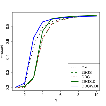
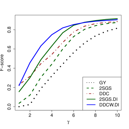
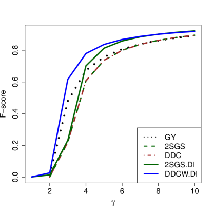
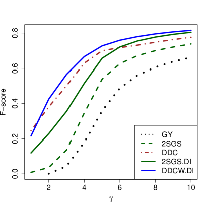
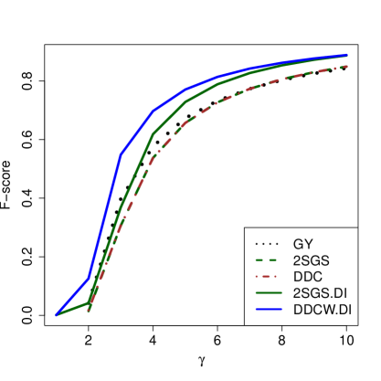
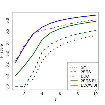
Figure 8: F-scores of flagged cellwise outliers on data generated by the contaminated ALYZ model (left) and the contaminated A09 model (right), for $(n,d)=(100,10)$ (top), $(n,d)=(400,20)$ (middle), and $(n,d)=(800,40)$ (bottom).

Appendix H Computation times of DI

Table 1 shows computation times of the DI algorithm as implemented in the R package cellWise on CRAN. This implementation contains compiled C++ code. The times are the averaged runtimes of one replication of the simulations in Figure 4 for $(n,d)=(100,10)$ and Figure 5 for $(n,d)=(400,20)$ and $(800,40)$. The times are in seconds on a laptop with Intel Core i7-5600U at 2.60Hz. We see that DDCW.DI requires less time than 2SGS.DI because the DDCW initial estimator is quite fast. Note that the computation time of the D-step in DI could be reduced by executing the LARS computations on the rows in parallel.

Table 1: Computation time (in seconds) of one replication of DI in the simulation.

$n$ and $d$	2SGS.DI	DDCW.DI
$n=100$, $d=10$	1.70	0.54
$n=400$, $d=20$	16.42	5.38
$n=800$, $d=40$	110.25	35.16

Appendix I Simulation with cellwise and casewise outliers

We now run a simulation in which the data are contaminated by $10\%$ of cellwise outliers generated as in the paper, plus $10\%$ of rowwise outliers. In this particular setting “rowwise outliers” refers to rows in which all cells are contaminated in the same way as before, that is, rows with $d$ cellwise outliers. We generate these outlying rows by the formula $\bm{v}=\gamma d\sqrt{d}\,\bm{u}^{\prime}/\operatorname{\mbox{MD}}(\bm{u},\bm{\mu},\bm{\Sigma})$ where $\bm{u}$ is the eigenvector of $\bm{\Sigma}$ with smallest eigenvalue. This corresponds to the cellwise formula of Subsection 2.3 in which the indices of the outlying cells $K=\{j(1),\ldots,j(k)\}$ are replaced by $K=\{1,\ldots,d\}$. Next, we replace 10% of the rows by $\bm{v}$, and afterward sample the positions of the cellwise outliers from the remaining 90% of the rows. The results are shown in Figures 9 and 10. They look qualitatively similar to those in Figures 4 and 5 in the paper.

ALYZ, 10% cells & 10% cases,
$\bm{d=10}$

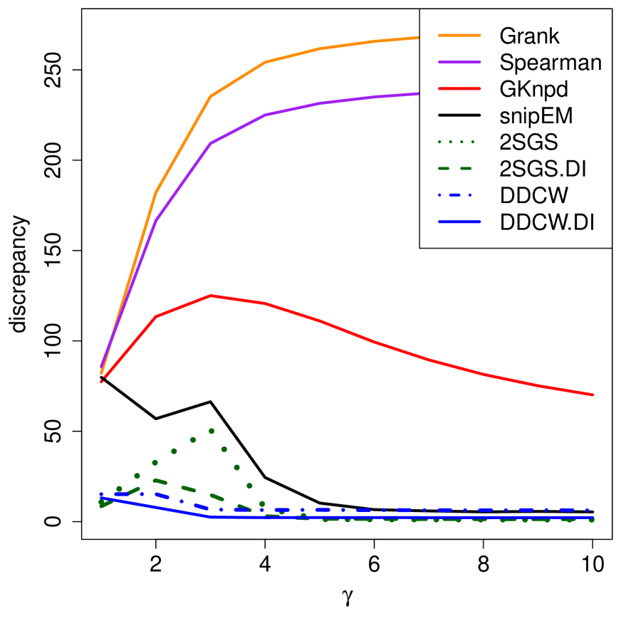
A09, 10% cells & 10% cases,
$\bm{d=10}$

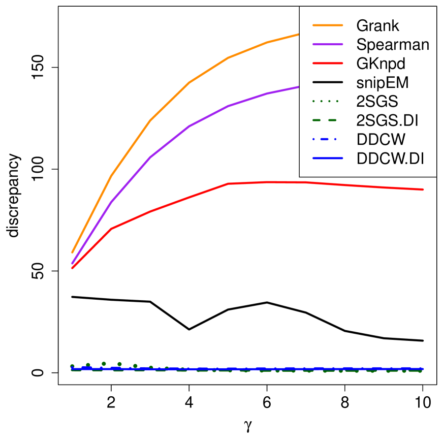
Figure 9: Discrepancy $D(\widehat{\bm{\Sigma}},\bm{\Sigma})$ of estimated covariance matrices for $d=10$, $n=100$.

ALYZ, 10% cells & 10% cases,
$\bm{d=20}$

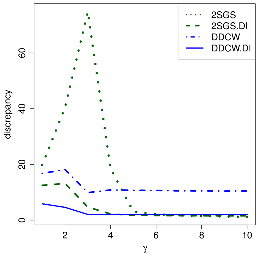
A09, 10% cells & 10% cases,
$\bm{d=20}$

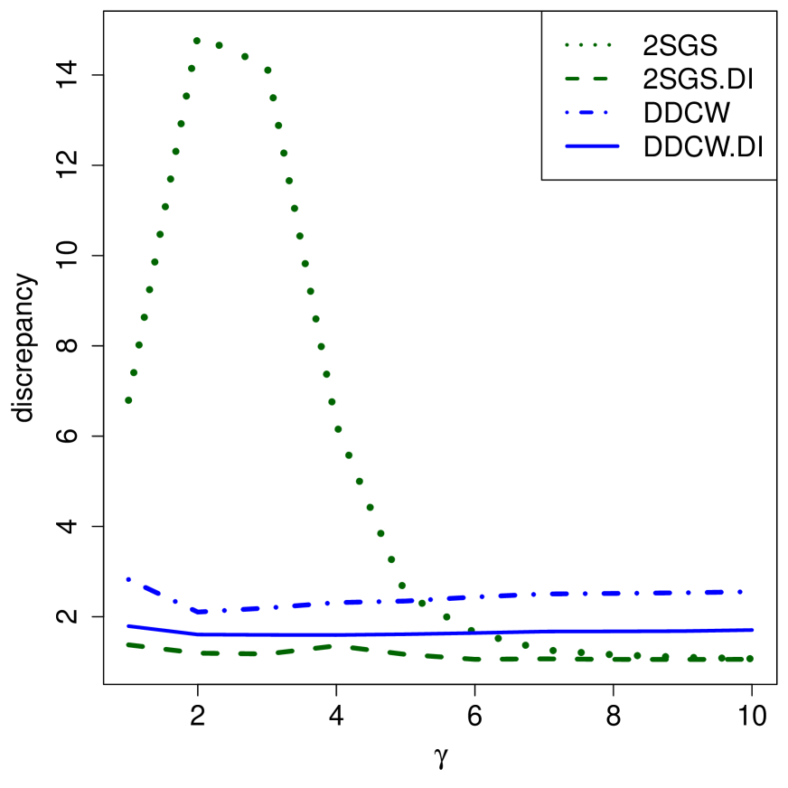
ALYZ, 10% cells & 10% cases,
$\bm{d=40}$

A09, 10% cells & 10% cases,
$\bm{d=40}$

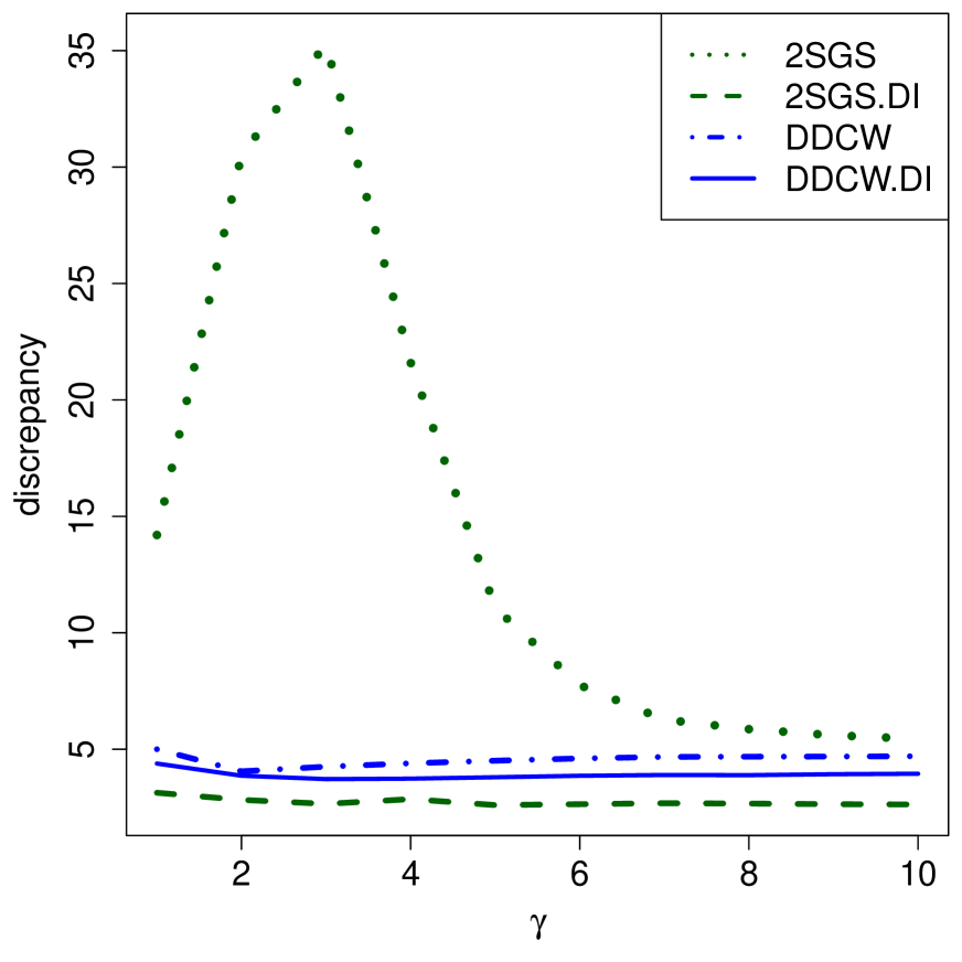
Figure 10: Discrepancy $D(\widehat{\bm{\Sigma}},\bm{\Sigma})$ given by (5) of estimated covariance matrices for $d=20$ and $n=400$ (top panels) and for $d=40$ and $n=800$ (bottom panels).

Note that in this section we do not plot F-scores for rowwise outliers, because the cellHandler and DI algorithms do not have a mechanism for detecting rowwise outliers. They are methods for cellwise outliers. If we were to try to detect both types of outliers simultaneously we would run into an identifiability issue. For instance, you can easily generate rows which would be considered outliers under the rowwise paradigm, but only contain a single cellwise outlier under the cellwise paradigm. And starting from the cellwise paradigm, how many cellwise outliers in a row would it take before the entire row should be considered outlying? The identifiability issue is especially complicated in the current simulations because we generate cellwise outliers in a structured way as explained in Section 2.3, so that they do not stand out individually.

Because of these concerns, when generating both types of outliers in this section our focus is on the accuracy of the covariance matrix estimate, so it is clear what the goal is. Afterward, the user can choose whether to employ the estimated covariance matrix to detect rowwise outliers based on their Mahalanobis-type distance, or as an input to the cellHandler algorithm to detect cellwise outliers.

Appendix J List of volatile organic compounds

The volatile organic compounds (VOC’s) analyzed in Section 6 are listed below.

Variable Name	VOC name
URX2MH	2-Methylhippuric acid
URX34M	3- and 4-Methylhippuric acid
URXAAM	N-Acetyl-S-(2-carbamoylethyl)-L-cysteine
URXAMC	N-Acetyl-S-(N-methylcarbamoyl)-L-cysteine
URXATC	2-Aminothiazoline-4-carboxylic acid
URXBMA	N-Acetyl-S-(benzyl)-L-cysteine
URXCEM	N-Acetyl-S-(2-carboxyethyl)-L-cysteine
URXCYM	N-Acetyl-S-(2-cyanoethyl)-L-cysteine
URXDHB	N-Acetyl-S-(3,4-dihydroxybutyl)-L-cysteine
URXHP2	N-Acetyl-S-(2-hydroxypropyl)-L-cysteine
URXHPM	N-Acetyl-S-(3-hydroxypropyl)-L-cysteine
URXIPM3	N-Acetyl- S- (4- hydroxy- 2- methyl- 2- butenyl)-L-cysteine
URXMAD	Mandelic acid
URXMB3	N-Acetyl-S-(4-hydroxy-2-butenyl)-L-cysteine
URXPHG	Phenylglyoxylic acid
URXPMM	N-Acetyl-S-(3-hydroxypropyl-1-methyl)-L-cysteine

Appendix K Analysis of the VOC data after preprocessing

As kindly pointed out by a referee, the concentrations of compounds in urine samples can depend on the dilution of the urine, if the analytical chemistry technique did not adjust for this. Therefore, the measurements might not always be comparable across the different samples. This issue can be dealt with by applying the centered log ratio (CLR) transform, which transforms the original data to log-ratios between the variables. We reran the analysis of the VOC data after applying the CLR transform using the cenLR function in the R-package robCompositions (Templ et al., , 2020).

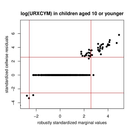
Figure 11: Plot of standardized cell residuals of CLR-transformed URXCYM obtained by cellHandler, versus the robustly standardized values of CLR-transformed URXCYM on its own.

Figures 11 and 12 present the results of this analysis. In the first plot we see that the univariate detection rule flags a few more outliers after the CLR transform than without it. However, the red curve in the second figure still shows no effect of adult smokers in the household on URXCYM in children. Therefore the conclusion that univariate outlier detection is insufficient here remains valid.

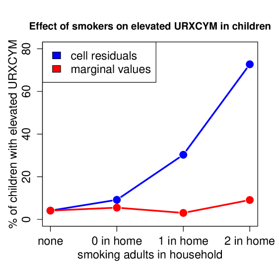
Figure 12: The blue curve shows the percentage of elevated URXCYM cell residuals in function of the smoking status of adult family members. The red curve shows the percentage of elevated marginal URXCYM values. Here the URXCYM values were preprocessed with the CLR transformation.

References

- Agostinelli et al., (2015) Agostinelli, C., Leung, A., Yohai, V. J., and Zamar, R. H. (2015). Robust estimation of multivariate location and scatter in the presence of cellwise and casewise contamination. TEST, 24:441–461, ISSN: 1863-8260, DOI: 10.1007/s11749-015-0450-6.
- Alqallaf et al., (2009) Alqallaf, F., Van Aelst, S., Yohai, V. J., and Zamar, R. H. (2009). Propagation of outliers in multivariate data. The Annals of Statistics, 37:311--331, DOI: 10.1214/07-AOS588.
- Chandola et al., (2009) Chandola, V., Banerjee, A., and Kumar, V. (2009). Anomaly detection: A survey. ACM Computing Surveys, 41:1--58, DOI: 10.1145/1541880.1541882.
- Chen et al., (2019) Chen, M., Carmella, S. G., Sipe, C., Jensen, J., Luo, X., Le, C. T., Murphy, S. E., Benowitz, N. L., McClernon, F. J., Vandrey, R., Allen, S. S., Denlinger-Apte, R., Cinciripini, P. M., Strasser, A. A., al’Absi, M., Robinson, J. D., Donny, E. C., Hatsukami, D., and Hecht, S. S. (2019). Longitudinal stability in cigarette smokers of urinary biomarkers of exposure to the toxicants acrylonitrile and acrolein. PLOS ONE, 14(1):1--13, DOI: 10.1371/journal.pone.0210104.
- Croux and Öllerer, (2016) Croux, C. and Öllerer, V. (2016). Robust and sparse estimation of the inverse covariance matrix using rank correlation measures. In Agostinelli, C., Basu, A., Filzmoser, P., and Mukherjee, D., editors, Recent Advances in Robust Statistics: Theory and Applications, pages 35--55, New Delhi. Springer India, DOI: 10.1007/978-81-322-3643-6_3.
- Danilov, (2010) Danilov, M. (2010). Robust estimation of multivariate scatter in non-affine equivariant scenarios. PhD thesis, University of British Columbia.
- Danilov et al., (2012) Danilov, M., Yohai, V. J., and Zamar, R. H. (2012). Robust estimation of multivariate location and scatter in the presence of missing data. Journal of the American Statistical Association, 107:1178--1186, DOI: 10.1080/01621459.2012.699792.
- Debruyne et al., (2019) Debruyne, M., Höppner, S., Serneels, S., and Verdonck, T. (2019). Outlyingness: Which variables contribute most? Statistics and Computing, 29:707--723, DOI: 10.1007/s11222-018-9831-5.
- Dice, (1945) Dice, L. R. (1945). Measures of the amount of ecologic association between species. Ecology, 26:297--302, DOI: 10.2307/1932409.
- Efron et al., (2004) Efron, B., Hastie, T., Johnstone, I., and Tibshirani, R. (2004). Least angle regression. The Annals of Statistics, 32:407--499, DOI: 10.1214/009053604000000067.
- Farcomeni, (2014) Farcomeni, A. (2014). Robust constrained clustering in presence of entry-wise outliers. Technometrics, 56(1):102--111, DOI: 10.1080/00401706.2013.826148.
- Farcomeni and Leung, (2019) Farcomeni, A. and Leung, A. (2019). Package snipEM: Snipping Methods for Robust Estimation and Clustering. CRAN, R package version 1.0.1, https://CRAN.R-project.org/package=snipEM.
- Gnanadesikan and Kettenring, (1972) Gnanadesikan, R. and Kettenring, J. R. (1972). Robust estimates, residuals, and outlier detection with multiresponse data. Biometrics, 28:81--124, ISSN: 0006341X, 15410420, http://www.jstor.org/stable/2528963.
- Hastie and Efron, (2015) Hastie, T. and Efron, B. (2015). Package lars: Least Angle Regression, Lasso and Forward Stagewise. CRAN, R package version 1.2, https://CRAN.R-project.org/package=lars.
- Higham, (2002) Higham, N. J. (2002). Computing the nearest correlation matrix - a problem from finance. IMA Journal of Numerical Analysis, 22:329--343, ISSN: 0272-4979, DOI: 10.1093/imanum/22.3.329.
- Leung et al., (2019) Leung, A., Danilov, M., Yohai, V., and Zamar, R. (2019). Package GSE: Robust Estimation in the Presence of Cellwise and Casewise Contamination and Missing Data. CRAN, R package version 4.2, https://CRAN.R-project.org/package=GSE.
- Leung et al., (2017) Leung, A., Yohai, V., and Zamar, R. (2017). Multivariate location and scatter matrix estimation under cellwise and casewise contamination. Computational Statistics & Data Analysis, 111:59--76, ISSN: 0167-9473, DOI: 10.1016/j.csda.2017.02.007.
- Little and Rubin, (1987) Little, R. and Rubin, D. (1987). Statistical Analysis with Missing Data. Wiley-Interscience, New York.
- Maronna et al., (2019) Maronna, R., Martin, D., Yohai, V., and Salibián-Barrera, M. (2019). Robust Statistics: Theory and Methods, Second Edition. Wiley, New York.
- NHANES, (2019) NHANES (2019). National Health and Nutrition Examination Survey Data. Hyattsville, MD: U.S. Department of Health and Human Services, Centers for Disease Control and Prevention. https://wwwn.cdc.gov/nchs/nhanes/.
- Öllerer and Croux, (2015) Öllerer, V. and Croux, C. (2015). Robust high-dimensional precision matrix estimation. In Nordhausen, K. and Taskinen, S., editors, Modern Nonparametric, Robust and Multivariate Methods: Festschrift in Honour of Hannu Oja, pages 325--350. Springer International Publishing, Cham, DOI: 10.1007/978-3-319-22404-6_19.
- Petersen and Pedersen, (2012) Petersen, K. B. and Pedersen, M. S. (2012). The Matrix Cookbook. Technical University of Denmark, http://www2.imm.dtu.dk/pubdb/pubs/3274-full.html.
- Raymaekers and Rousseeuw, (2019) Raymaekers, J. and Rousseeuw, P. J. (2019). Fast robust correlation for high-dimensional data. DOI: 10.1080/00401706.2019.1677270. Technometrics, published online, open access.
- Raymaekers et al., (2020) Raymaekers, J., Rousseeuw, P. J., Van den Bossche, W., and Hubert, M. (2020). Package cellWise: Analyzing Data with Cellwise Outliers. CRAN, R package version 2.2.2, https://CRAN.R-project.org/package=cellWise.
- Rousseeuw and Croux, (1993) Rousseeuw, P. J. and Croux, C. (1993). Alternatives to the median absolute deviation. Journal of the American Statistical Association, 88:1273--1283, DOI: 10.1080/01621459.1993.10476408.
- Rousseeuw and Van den Bossche, (2018) Rousseeuw, P. J. and Van den Bossche, W. (2018). Detecting deviating data cells. Technometrics, 60:135--145, DOI: 10.1080/00401706.2017.1340909. Open access.
- Tarr et al., (2016) Tarr, G., Müller, S., and Weber, N. (2016). Robust estimation of precision matrices under cellwise contamination. Computational Statistics & Data Analysis, 93:404--420, ISSN: 0167-9473, DOI: 10.1016/j.csda.2015.02.005.
- Templ et al., (2020) Templ, M., Hron, K., and Filzmoser, P. (2020). Package robCompositions: Compositional Data Analysis. CRAN, R package version 2.2.1, https://CRAN.R-project.org/package=robCompositions.
- Tibshirani, (1996) Tibshirani, R. (1996). Regression shrinkage and selection via the lasso. Journal of the Royal Statistical Society Series B, 58:267--288, https://www.jstor.org/stable/2346178.
- Unwin, (2019) Unwin, A. (2019). Multivariate outliers and the O3 plot. Journal of Computational and Graphical Statistics, 28:635--643, DOI: 10.1080/10618600.2019.1575226.
- Van Aelst et al., (2011) Van Aelst, S., Vandervieren, E., and Willems, G. (2011). Stahel-Donoho estimators with cellwise weights. Journal of Statistical Computation and Simulation, 81(1):1--27, DOI: 10.1080/00949650903103873.