Efficient Top-k Vulnerable Nodes Detection in Uncertain Graphs

Abstract

Uncertain graphs have been widely used to model complex linked data in many real-world applications, such as guaranteed-loan networks and power grids, where a node or edge may be associated with a probability. In these networks, a node usually has a certain chance of default or breakdown due to self-factors or the influence from upstream nodes. For regulatory authorities and companies, it is critical to efficiently identify the vulnerable nodes, i.e., nodes with high default risks, such that they could pay more attention to these nodes for the purpose of risk management. In this paper, we propose and investigate the problem of top-$k$ vulnerable nodes detection in uncertain graphs. We formally define the problem and prove its hardness. To identify the $k$ most vulnerable nodes, a sampling-based approach is proposed. Rigorous theoretical analysis is conducted to bound the quality of returned results. Novel optimization techniques and a bottom-$k$ sketch based approach are further developed in order to scale for large networks. In the experiments, we demonstrate the performance of proposed techniques on 3 real financial networks and 5 benchmark networks. The evaluation results show that the proposed methods can achieve up to 2 orders of magnitudes speedup compared with the baseline approach. Moreover, to further verify the advantages of our model in real-life scenarios, we integrate the proposed techniques with our current loan risk control system, which is deployed in the collaborated bank, for more evaluation. Particularly, we show that our proposed new model has superior performance on real-life guaranteed-loan network data, which can better predict the default risks of enterprises compared to the state-of-the-art techniques.

Keywords Uncertain graph  $\cdot$ guaranteed-loan network  $\cdot$ top-$k$  $\cdot$ vulnerable node detection

1 Introduction

Uncertainty is inherent in real-world data because of various reasons, such as the accuracy issue of devices and models [DBLP:conf/icde/LiDWMQY19, DBLP:journals/tkde/ZhangLZZZ16]. Sometimes, people may inject uncertainty to the data on purpose to protect user privacy [DBLP:journals/pvldb/BoldiBGT12]. As a common data structure, graphs are widely used to model the complex relationships between different entities. Due to the ubiquitous uncertainty, uncertain graph analysis has attracted significant attentions in the community of database management. A large number of graph problems have been studied in the context of uncertain graphs, e.g., nearest neighbor search [potamias2010k], reliability query [ke2019depth], cohesive subgraph mining [DBLP:conf/icde/LiDWMQY19], etc.

In some real-life graphs, such as power grids and guaranteed-loan networks, nodes (e.g., facilities and enterprises) may breakdown or default due to self-factors or the issues from upstream nodes. To identify these high-risky (i.e., vulnerable) nodes, in this paper, we investigate a novel problem, named top-$k$ vulnerable nodes detection. Given a directed uncertain graph $\mathcal{G}$, each node $A$ (resp. edge $(A,B)$) is associated with a probability $p_{s}(A)$ (resp. $p(B|A)$). $p_{s}(A)$ denotes the probability that $A$ defaults due to itself factors, and $p(B|A)$ denotes the probability that $B$ defaults because of the default of $A$. By considering both factors, we can calculate the node default probability. We say a node is more vulnerable if it has higher default probability. The problem is different from the existing research, such as reliability problem and influence maximization problem [ke2019depth, li2018influence], which more focus on investigating the reachability for a set of nodes or finding a group of nodes to maximize the influence over the network. Our problem is of great importance to many real-world applications. Following is a motivating example on financial data analysis.

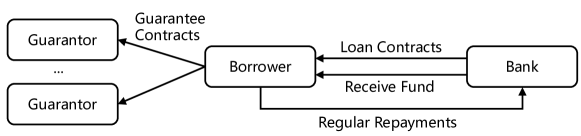
Figure 1: Guarantee loan process

Motivating application. Network-guaranteed loan (also known as guarantee circle) is a widespread economic phenomenon, and attracting increasing attention from the banks, financial regulatory authorities, governments, etc. In order to obtain loans from banks, groups of small and medium enterprises (SMEs) back each other to enhance their financial security. Figure 1 shows the flow of guarantee loan procedure. When more and more enterprises are involved, they form complex directed-network structures [cheng2020delinquent]. Figure 2 illustrates a guaranteed-loan network with around $3,000$ enterprises and $7,000$ guarantee relations, where a node represents a small or medium enterprise and a directed edge from node $A$ to node $B$ indicates that enterprise $B$ guarantees another enterprise $A$. Thousands of guaranteed-loan networks of different complexities have coexisted for a long period [jian2012determinants]. It requires an efficient strategy to prevent, identify and dismantle systematic crises.

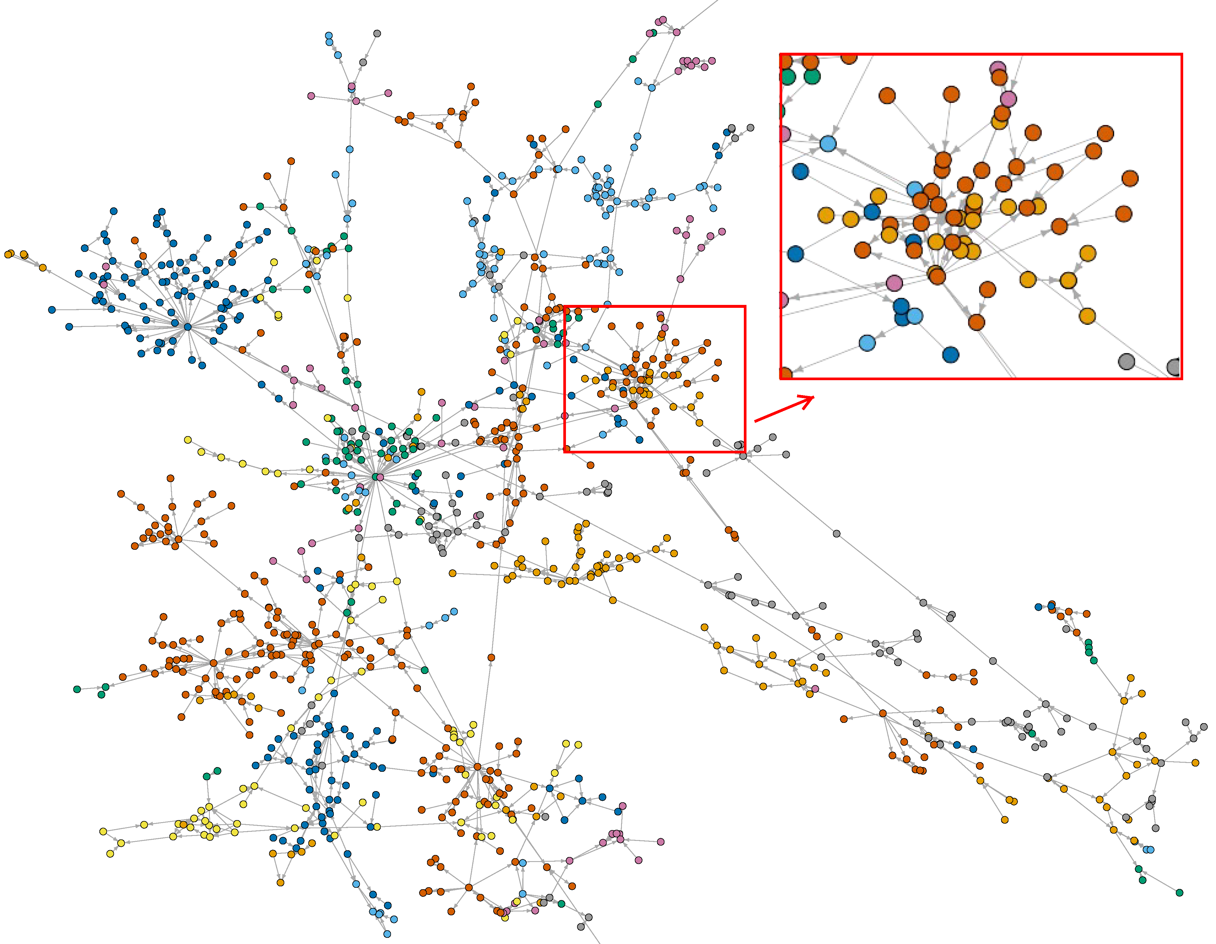
Figure 2: A real-world guaranteed-loan network

Many kinds of risk factors have emerged throughout the guaranteed-loan network, which may accelerate the transmission and amplification of risk. The guarantee network may be alienated from the “mutual aid group” as a “breach of contract”. An appropriate guarantee union may reduce the default risk, but significant contagion damage throughout the networked enterprises could still occur in practice [mcmahon2014loan]. The guaranteed loan is a debt obligation promise. If one corporation gets trapped in risks, it will spread the contagion to other corporations in the network. When defaults diffuse across the network, a systemic financial crisis may occur. It is essential to consider the contagion damage in the guaranteed-loan networks. We can model a guaranteed-loan network with our uncertain graph model, where each node has a self-risk probability and each edge has a risk diffusion probability. Figure 3(a) is toy example of guaranteed-loan network, where Figure 3(e) shows the corresponding relationships between different enterprises and the risk diffusion probabilities. It is desirable to efficiently identify the $k$ most vulnerable nodes, i.e., enterprises with high default risks, such that the banks or the financial regulatory authorities can pay extra attention to them for the purpose of risk management. It is more urgent than ever before with the slowdown of the economics worldwide nowadays.

In the literature, some machine-learning based approaches (e.g., [DBLP:conf/ijcai/ChengTMN019]) have been proposed to predict the node default risk for different applications. For instance, a high-order and graph attention based network representation method has been designed in [DBLP:conf/ijcai/ChengTMN019] to infer the possibility of loan default events. These approaches indeed consider the structure of networks. However, they cannot properly capture the uncertain nature of contagious behaviors in the networks. In the experiment, we also compare with these approaches to demonstrate the advantages of our model.

Our approach. In this paper, to identify the top-$k$ vulnerable nodes, we model the problem with an uncertain graph, and infer the default probability of a node following the possible world semantics, which has been widely used to capture the contagious phenomenon in real networks [DBLP:conf/sigmod/AbiteboulKG87, niu2020iconviz, DBLP:conf/ijcai/ChengWZ020, DBLP:conf/kdd/KempeKT03]. In particular, we utilize an uncertain graph with two types of probabilities to model the occurrence and prorogation of the default risks in the network. Note that, we focus on identifying vulnerable nodes for a given network, while the self-risk probabilities and diffusion probabilities can be obtained based on the existing works (e.g., [cheng2018prediction, DBLP:conf/ijcai/ChengTMN019]).

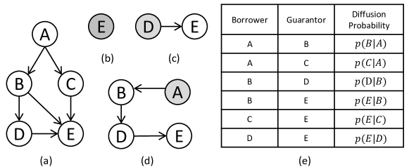
Figure 3: Example of uncertain guaranteed-loan network

Specifically, Figures 3(a) and 3(e) illustrate the structure of a toy uncertain graph with $5$ nodes and $6$ edges, as well as the associated self-risk probabilities and diffusion probabilities. Given the probabilistic graph $\mathcal{G}$, we may derive the default probability of a node following the possible world semantics, where each possible world (i.e., instance graph in this paper) corresponds to a subgraph (i.e., possible occurrence) of $\mathcal{G}$. Figures 3(b)-(d) are three example possible worlds of Figure 3(a). In each possible world, a node exits if it defaults, and an edge $(A,B)$ appears if the default of $A$ indeed leads to the default of $B$. Taking node $E$ as an example, it may default because of $(i)$ itself, which is represented by a shaded node as shown in Figure 3(b), or because of $(ii)$ the contagion damage initiated by other nodes as shown in Figures 3(c)-(d). In Section 2, we will formally introduce how to derive the default probabilities of nodes.

In this paper, we show that the problem of calculating the default probability of a node alone is #P-hard, not mentioning the top-$k$ vulnerable nodes identification problem. A straightforward solution for the top-$k$ vulnerable nodes computation is to enumerate all possible worlds and then aggregate the results in each possible world. However, it is computational prohibitive, since the number of possible worlds of an uncertain graph may be up to $2^{n+m}$, where $n$ and $m$ are the number of nodes and edges in the graph, respectively. In this paper, we first show that we can identify the top-$k$ vulnerable nodes by using a limited number of sampled instance graphs with tight theoretical guarantee. To reduce the sample size required and speedup the computation, lower/upper bounds based pruning strategies and advanced sampling method are developed. In addition, to further accelerate the computation, a bottom-$k$ sketch based method is proposed. To verify the performance in real scenarios, we integrate the proposed techniques with our current loan risk control system, which is deployed in the collaborated bank.

Contributions. The principle contributions of this paper are summarized as follows.

• We advocate the problem of top-$k$ vulnerable nodes detection in uncertain graphs, which is essential in real-world applications.

• Due to the hardness of the problem, a sampling based method is developed with tight theoretical guarantee.

• We develop effective lower and upper bound techniques to prune the searching space and reduce the sample size required. Advanced sampling method is designed to speed up the computation with rigorous theoretical analysis.

• A bottom-$k$ sketch based approach is further proposed, which can greatly speedup the computation with competitive results.

• We conduct extensive experiments to evaluate the efficiency and effectiveness of our proposed algorithms on $3$ real financial networks and $5$ benchmark networks.

• To further verify the advantages of our models in real scenarios, the proposed techniques are integrated into our current loan risk control system, which is deployed in the collaborated bank. Through the case study on real-life financial environment, it verifies that our proposed model can significantly improve the accuracy for high-risky enterprises prediction.

Roadmap. The rest of the paper is organized as follows. Section 2 describes the problem studied and the related techniques used in the paper. Section 3 shows the basic sampling-based method and our optimized algorithms. We report the experiment results in Section LABEL:sec:experiment. Section LABEL:sec:dep introduces the system implementation details and case study. We present the related work in Section LABEL:subsec:related_work and conclude the paper in Section LABEL:sec:conclusion.

Table 1: Summary of notations

Notation	Definition
$\mathcal{G}=(\mathcal{V},\mathcal{E})$	uncertain graph
$\mathcal{V}$/$\mathcal{E}$	node/edge set of $\mathcal{G}$
$p_{s}(v)$	the self-risk probability of $v$
$p(v_{i}|v_{j})$	the diffusion probability
$p(v)$	the default probability of $v$
$h(x)$	a truly random hash function
$\mathcal{L}(A,k)$	the $k$-th smallest hash value of the set $A$
$bk$	the parameter $k$ in the bottom-$k$ sketch
$N(v)$	the set of in-neighbors of node $v$
$\mathcal{A}$	an approximation algorithm for the problem
$\mathcal{R}$	the set of $k$ nodes returned by $\mathcal{A}$
$P^{k}$	the default probability of rank $k$-th nodes
$(\epsilon,\delta)$	the parameters in $(\epsilon,\delta)$-approximation
$t$	the sample size
$p_{l}(v)$, $p_{u}(v)$	the lower and upper bound of $p(v)$
$T_{l}$, $T_{u}$	the $k$-th largest value of $p_{l}(v)$ and $p_{u}(v)$
$\mathcal{B}$	the set of candidates
$\mathcal{G}^{t}$	graph by reversing the direction of edges in $\mathcal{G}$

2 Preliminaries

In this section, we first we present some key concepts and formally define the problem. Then, we introduce the related techniques used. Table 1 summarizes the notations frequently used throughout this paper.

2.1 Problem Definition

We consider an uncertain graph $\mathcal{G}=(\mathcal{V},\mathcal{E})$ as a directed graph, where $\mathcal{V}$ is the set of nodes and $\mathcal{E}$ denotes the set of edges. $n=|\mathcal{V}|$ (resp. $m=|\mathcal{E}|$) is the number of nodes (resp. edges) in $\mathcal{G}$. Each node $v\in\mathcal{V}$ is associated with a self-risk probability $p_{s}(v)$, which denotes the default probability of $v$ caused by self-factors. Each edge $(u,v)\in\mathcal{E}$ is associated with a diffusion probability $p(v|u)$, which denotes the probability of $v$’s default caused by $u$’s default. In this paper, we assume the self-risk probabilities and diffusion probabilities are already available. These probabilities can be derived based the previous studies (e.g., [DBLP:conf/ijcai/ChengTMN019]).

For simplicity, when there is no ambiguity, we use uncertain graph, graph and network interchangeably. In this paper, we derive the default probability of a node by considering both self-risk probability and diffusion probability, which is defined as follows.

Definition 1 (Default Probability).

Given an uncertain graph $\mathcal{G}=(\mathcal{V},\mathcal{E})$, for each node $v\in\mathcal{V}$, its default probability, denoted by $p(v)$, is obtained by considering both self-risks probability and diffusion probability. $p(v)$ can be computed recursively as follows.

$$p(v)=1-(1-p_{s}(v))\left(\prod_{~{}all~{}x\in N(v)}\left(1-p(v|x)p(x)\right)\right)$$ (1)

where $N(v)$ is the set of in-neighbors of $v$.

It is easy to verify that the equation above is equal to aggregate the probability over all the possible worlds, i.e.,

$$p(v)=\sum_{W\in\mathcal{W}}p(W)\times I_{W}(v)$$

where $\mathcal{W}$ is the set of all possible worlds, $p(W)$ is the probability of a possible world $W$, and $I_{W}(v)$ is an indicator function denoting if $v$ defaults in $W$ or not.

Example 1.

Reconsider the graph in Figure 3. Suppose the self-risk probabilities and diffusion probabilities are all 0.2 for each node and edge. Then, we have $p(A)=0.2$ and $p(B)=1-(1-p_{s}(B))(1-0.2\times p(A))=0.232$.

Problem statement. Given an uncertain graph $\mathcal{G}=(\mathcal{V},\mathcal{E})$, we aim to develop efficient algorithms to identify the set $\mathcal{R}$ of top-$k$ vulnerable nodes, i.e., the $k$ nodes with the highest default probability.

Theorem 1.

It is #P-hard to compute the default probability.

Proof.

We show the hardness of the problem by considering a simple case, where the self-risk probability $p_{s}(v)$ equals 1 for node $v$, and $p_{s}(u)$ equals 0 for $u\in\mathcal{V}\setminus v$. Therefore, for the node $u\in\mathcal{V}\setminus v$, the default probability $p(u)$ is only caused by the default of node $v$. Then, the default probability of $p(u)$ equals the reliability from $v$ to $u$, which is #P-hard to compute [khan2014fast]. Thus, it is #P-hard to compute the default probability. The theorem is correct. ∎

2.2 Bottom-k Sketch

In this section, we briefly introduce the bottom-$k$ sketch [cohen2007summarizing], which is used in our BSRBKframework to obtain the statistics information for early stopping condition. Bottom-$k$ sketch is designed for estimating the number of distinct values in a multiset. Given a multiset $A=\{v_{1},v_{2},\cdots,v_{n}\}$ and a truly random hash function $h$, each distinct value $v_{i}$ in the set $A$ is hashed to $(0,1)$ and $h(v_{i})\neq h(v_{j})$ for $i\neq j$. The bottom-$k$ sketch consists of the $k$ smallest hash values, i.e., $\mathcal{L}(A)=\{h(v_{i})|h(v_{i})\leq\mathcal{L}(A,k)\wedge v_{i}\in A\}$, where $\mathcal{L}(A,k)$ is the $k$-th smallest hash value. So the number of distinct value can be estimated with $\frac{k-1}{\mathcal{L}(A,k)}$. The estimation can converge fast with the increase of $k$, where the expected relative error is $\sqrt{2/{\pi(k-2)}}$ and the coefficient variation is no more than $1/\sqrt{k-2}$. To distinguish from the $k$ in the top-$k$ problem, hereafter in this paper, we use $bk$ to denote the parameter $k$ in the bottom-$k$ sketch.

3 Solutions

In this section, we first present a basic sampling method and analyze the sample size required. Then, we introduce the optimized approaches to accelerate the processing.

3.1 Basic Sampling Approach

Due to the hardness of computing the default probability, in this section, we propose a sampling based method. In order to bound the worst case performance, rigorous theoretical analysis is conducted about the required sample size.

Sampling framework. To compute the default probability, we can enumerate all the possible worlds and aggregate the results. However, the possible world space is usually very large. In previous research, sampling based methods are widely adopted for this case. That is, we randomly select a set of possible worlds and take the average value as the estimated default probability. By carefully choosing the sample size, we can return a result with performance guarantee.

Algorithm 1 shows the details of the basic sampling based method. The input is a given graph, where each node/edge is associated with a self-risk/diffusion probability. In each iteration, we generate a random number for each node to determine if it defaults by itself or not (Lines 4-7). Then, we conduct a breath first search from these nodes, i.e., $h_{v}=1$, to locate the nodes that will be influenced by them in the current simulation. For each encountered edge, we generate a random number to decide if the propagation will continue or not. For each node, the number of default times is accumulated in Lines 21. The final default probability is calculated by taking an average over the accumulated value $v^{c}$. Finally, the algorithm returns $k$ results with the largest estimated value.

Example 2.

Reconsider the example in Figure 3. Suppose Figures 3(b)-3(d) are the three sampled graphs, and nodes $E,D,A$ are the ones default by itself. Assuming $k=2$, then, nodes $E$ and $D$ are returned results with the largest estimated default probabilities.

Input :  $\mathcal{G}:$ a given graph, $k$: a positive integer, $t$: sample size

Output : $\mathcal{R}$: collection of top-$k$ vulnerable nodes

$u_{v}:=0$ for all nodes $v\in\mathcal{V}$ ;AlgoLine0.1

for $i$ in $1$ to $t$ do  $h_{v}:=0$ for all nodes $v\in\mathcal{V}$; AlgoLine0.2

for each $v\in\mathcal{V}$ do  generate a random number $r_{v}$ in $[0,1]$; AlgoLine0.3

if $r_{v}\leqslant p_{s}(v)$ then  $h_{v}:=1$; AlgoLine0.4

    AlgoLine0.5

$\mathcal{Q}\leftarrow\{v|h_{v}=1\}$ ;AlgoLine0.6

mark $\mathcal{V}\setminus\mathcal{Q}$ as unvisited ;AlgoLine0.7

AlgoLine0.8

while $\mathcal{Q}\neq\emptyset$ do  $v_{q}\leftarrow\mathcal{Q}.pop()$ ; AlgoLine0.9

for each $v_{a}\in N(v_{q})$ do  if $v_{a}$ is unvisited then  generate a random number $r_{e}$ in $[0,1]$ ; AlgoLine0.10

if $r_{e}>p(v_{a}|v_{q})$ then  continue ; AlgoLine0.11

  $h_{v_{a}}:=1$ ;AlgoLine0.12

mark $v_{a}$ as visited ;AlgoLine0.13

push $v_{a}$ to $\mathcal{Q}$ ;AlgoLine0.14

      for each $v\in\mathcal{V}$ do  $v^{c}:=v^{c}+h_{v}$ ; AlgoLine0.15

    $\mathcal{R}\leftarrow$ the top-$k$ nodes ordered by $p_{v}=v^{c}/t$ ;AlgoLine0.16

return $\mathcal{R}$

Algorithm 1 Basic Sampling Approach

16

16

16

16

16

16

16

16

16

16

16

16

16

16

16

16

Sample size analysis. For sampling based methods, a critical problem is to determine the sample size required in order to bound the quality of returned result. In this section, we conduct rigorous theoretical analysis about the sample size required. Specifically, we say an algorithm $\mathcal{A}$ is $(\epsilon,\delta)$-approximation if the following conditions hold.

Definition 2 ($(\epsilon,\delta)$-approximation).

Given an approximation algorithm $\mathcal{A}$ for the top-$k$ problem studied, let $\mathcal{R}$ be the set of $k$ nodes returned by $\mathcal{A}$. $P^{k}$ is the default probability of the $k$-th node in the ground truth order. Given $\epsilon,\delta\in(0,1)$, we say $\mathcal{A}$ is $(\epsilon,\delta)$-approximation if $\mathcal{R}$ fulfills the following conditions with at least $1-\delta$ probability.

• For $v\in\mathcal{R}$, $p(v)\geq P^{k}-\epsilon$;

• For $v\notin\mathcal{R}$, $p(v)<P^{k}+\epsilon$.

If $\mathcal{A}$ is a $(\epsilon,\delta)$-approximation algorithm for the vulnerable node detection problem, it means that with high probability $(i)$ the default probabilities of returned nodes are at least $P_{v}^{k}-\epsilon$; $(ii)$ for the nodes not in $\mathcal{R}$, the default probabilities are at most $P^{k}+\epsilon$.

Theorem 2 (Hoeffding Inequality).

Given a sample size $t$ and $\epsilon>0$, let ${p_{v}}$ be the unbiased estimation of $p(v)$, where $p_{v}=\frac{1}{t}\sum_{i=1}^{t}p_{v}^{i}$ and $p_{v}^{i}\in[a^{i},b^{i}]$. Then we have

$$Pr[{p_{v}}-p(v)\geq\epsilon]\leq\exp(-\frac{2t^{2}\epsilon^{2}}{\sum_{i=1}^{t}(a^{i}-b^{i})^{2}})$$ (2)

Based on the Hoeffding inequality, we have following theorem hold.

Theorem 3.

Given the sample size $t$, $\epsilon>0$ and two nodes $u,v\in\mathcal{V}$, if $p(v)-p(u)\geq\epsilon$, then

$$Pr[{p_{u}}-{p_{v}}>0]\leq\exp(-t\epsilon^{2}/2)$$

Proof.

We have

$$Pr[{p_{u}}-{p_{v}}>0]$$

$$\leq~{} Pr[{p_{u}}-{p_{v}}\geq p(u)-p(v)-\epsilon]$$

$$=~{} Pr[{p_{u}}-{p_{v}}-(p(u)-p(v))\geq\epsilon]$$

$$\leq~{} \exp(-\frac{2t^{2}\epsilon^{2}}{\sum_{i=1}^{t}2^{2}})$$

$$=~{} \exp(-t\epsilon^{2}/2)$$

The last two steps consider ${p_{u}}-{p_{v}}$ as the estimator of $p(u)-p(v)$. In addition, $p_{u}^{i}-p_{v}^{i}\in[-1,1]$. Then, we can feed into the Hoeffding inequality and obtain the final result. ∎

As shown in Theorem 4, Algorithm 1 is a $(\epsilon,\delta)$-approximation algorithm if the sample size is no less than Equation 3.

Theorem 4.

Algorithm 1 is $(\epsilon,\delta)$-approximation if the sample size is no less than

$$t=\frac{2}{\epsilon^{2}}\ln{\frac{k(n-k)}{\delta}}$$ (3)

where $n$ is the number of nodes, i.e., $|\mathcal{V}|$.

Proof.

Suppose we sort the nodes based on their real default probabilities, i.e., $\{v_{1},v_{2},...,v_{n}\}$. Then we show the two conditions in $(\epsilon,\delta)$-approximation hold if we have $p_{v_{i}}-p_{v_{j}}>0$ with $p(v_{i})-p(v_{j})\geq\epsilon$ for $1\leq i\leq k<j\leq n$.

• For a node $v\in\mathcal{R}$, if $p(v)<P^{k}-\epsilon<p(v_{i})-\epsilon$, it means $p_{v_{i}}-p_{v}>0$ for $i\in[1,k]$. Therefore, $v$ will not be selected into $\mathcal{R}$, which is contradict to the assumption. Thus, the first condition holds.

• For $v\notin\mathcal{R}$, if $v$ does not belong to the top-$k$ result, the second condition holds naturally. Otherwise, there must be a node $u$ that does not belong to the top-$k$ result being selected into $\mathcal{R}$. If $p(v)\geq P^{k}+\epsilon\geq p(u)+\epsilon$, it means $p_{v}-p_{u}>0$. Therefore, $v$ should also be selected into the top-$k$, which is contradict to the assumption. Thus, the second condition holds.

Theorem 3 shows the theoretical result of bounding the order of a pair of nodes. Since $1\leq i\leq k<j\leq n$, we need to bound the order of $k(n-k)$ pairs of nodes. By applying union bound and Theorem 3, we have

$$\delta=k(n-k)\exp(-t\epsilon^{2}/2)$$

$$\Rightarrow t=\frac{2}{\epsilon^{2}}\ln{\frac{k(n-k)}{\delta}}$$

Therefore, the theorem is correct. ∎

3.2 Optimized Sampling Approach

Based on Theorem 4, Algorithm 1 can return a result with tight theoretical guarantee. However, it still suffers from some drawbacks, which make it hard to scale for large graphs. Firstly, to bound the quality of returned results, we need to bound the order of $k(n-k)$ node pairs. The node size $n$ can be treated as the candidate size, which is usually large in real networks. Therefore, if we can reduce the size of $n$ (i.e., reduce candidate space) and $k$ (i.e., verify some nodes without estimation), then the sample size can be reduced significantly. Secondly, in each sampled possible world, we only need to determine whether the candidate node can be influenced or not, i.e., compute $h_{v}$. If the candidate space can be greatly reduced, the previous sampling method may explore a lot of unnecessary space.

According to the intuitions above, in this section, novel methods are developed to derive the lower and upper bounds of the default probability, which are used to reduce the candidate space. In addition, a reverse sampling framework is proposed in order to reduce the searching cost.

Input :  $\mathcal{G}:$ a given graph, $z$: the order of bound

Output :  $p_{l}(v)$: lower bound of default probability

for $i$ in $1$ to $z$ do  if $i=1$ then  $p(v):=p_{s}(v)$ for each $v\in\mathcal{V}$; AlgoLine0.1

continue;AlgoLine0.2

  for each $v$ in $\mathcal{V}$ do  calculate $p(v)$ by Equitation 1 if its in-neighbors’ default probabilities have been updated in the previous iteration; AlgoLine0.3

    $p_{l}(v):=p(v)$ for all nodes $v\in\mathcal{V}$;AlgoLine0.4

return $p_{l}(v)$ for $v\in\mathcal{V}$

Algorithm 2 Lower Bound Algorithm

4

4

4

4

Candidate size reduction. To compute the lower and upper bounds of the default probability, we utilize the equation in default probability definition, i.e., Equation 1. The idea is that the default probability for each node is in $[p_{s}(v),1]$ if no further information is given. By treating each node’s default probability as $p_{s}(v)$ and $1$, we can aggregate the probability over its neighbors to shrink the interval based on Equation 1. Then, with the newly derived lower and upper bounds for neighbor nodes, we can further aggregate the information and update the bounds. The details of deriving lower and upper bounds are shown in Algorithms 2 and 3. The algorithms iteratively use the lower and upper bound derived in the previous iteration as the current default probability. The order of bound denotes the number of iterations conducted. In each iteration, we only update the bounds of $v$’s default probability if there is any change for the default probability of $v$’s in-neighbors. Note that, there is a slight difference in the first iteration for the two algorithms, since by using 1 as the default probability will contribute nothing for the pruning. It is easy to verify that larger order will lead to tighter bounds. Users can make a trade-off between the efficiency and the tightness of bounds.

Given the lower bound and upper bound derived, we can filter some unpromising candidates and verify some candidates with large probability. Lemma 1 shows the pruning rules to verify and filter the candidate space.

Lemma 1.

Given the upper and lower bounds derived for each node, let $T_{l}$ and $T_{u}$ be the $k$-th largest value in $p_{l}(v)$ and $p_{u}(v)$, respectively. Then, we have

• For $u\in\mathcal{V}$, $u$ must be in the top-$k$ if $p_{l}(u)\geq T_{u}$.

• For $u\in\mathcal{V}$, $u$ must not be in the top-$k$ if $p_{u}(u)<T_{l}$.

Proof.

For the first case, suppose a node $u$ with $p_{l}(u)\geq T_{u}$ but not being selected in the top-$k$ results, which means a node must have default probability of at least $p_{l}(u)$ to be selected into the top-$k$ result. Since $T_{u}$ is the $k$-th largest value in $p_{u}(v)$, it means there will be no more than $k$ nodes that satisfy the condition. Therefore, the first case holds. For the second case, since $T_{l}$ is the $k$-th largest value of $p_{l}(v)$, which means $P^{k}$ must be at least $T_{l}$. Note that, $P^{k}$ is default probability of the ranked $k$-th node in the the ground truth order. Therefore, the second case holds. ∎

Input :  $\mathcal{G}:$ a given graph, $z$: the order of bound

Output :  $p_{u}(v)$: upper bound of default probability

for $i$ in 1 to $z$ do  for each vertex $v$ in $\mathcal{V}$ do  if $i=1$ then  calculate $p(v)$ by treating its in-neighbors’ default probabilities as 1; AlgoLine0.1

  else  calculate $p(v)$ if its in-neighbors’ default probabilities have been updated in the previous iteration; AlgoLine0.2

      $p_{u}(v):=p(v)$ for all nodes $v\in\mathcal{V}$;AlgoLine0.3

return $p_{u}(v)$ for $v\in\mathcal{V}$

Algorithm 3 Upper Bound Algorithm

3

3

3

Input :  $p_{u}(v)/p_{l}(v)$: upper and lower bound for each node, $k$: a positive integer

Output :  $\mathcal{B}$: candidates selected, $k^{\prime}$: the number of nodes verified

$T_{l}$ $\leftarrow$ the $k$-th largest value in $p_{l}(v)$ ;AlgoLine0.1

$T_{u}\leftarrow$ the $k$-th largest value in $p_{u}(v)$ ;AlgoLine0.2

$\mathcal{B}:=\emptyset$; $k^{\prime}=0$ ;AlgoLine0.3

for each $v$ in $\mathcal{V}$ do  if $p_{l}(v)\geq T_{u}$ then  $k^{\prime}++$; AlgoLine0.4

insert $v$ into the result set;AlgoLine0.5

continue;AlgoLine0.6

  AlgoLine0.7

if $p_{u}(v)\geq T_{l}$ then  push $v$ into $\mathcal{B}$ ; AlgoLine0.8

    return $\mathcal{B}$ and $k^{\prime}$

Algorithm 4 Candidate Reduction

8

8

8

8

8

8

8

8

Input :  $\mathcal{G}^{t}:$ a given graph by reverse the direction each edge, $\mathcal{B}$: candidate nodes

Output : $h_{v}$: for each node $v\in\mathcal{B}$ in one sample

$h_{v}:=0$ for all nodes $v\in\mathcal{V}$ ;AlgoLine0.1

for each node $v$ in $\mathcal{B}$ do  mark all nodes as unvisited ;AlgoLine0.2

$\mathcal{Q}\leftarrow\{v\}$ ;AlgoLine0.3

while $\mathcal{Q}\neq\emptyset$ do  $u=\mathcal{Q}.pop()$ ;AlgoLine0.4

if $h_{u}=1$ then  $h_{v}:=1$ and break ; AlgoLine0.5

  if $u$ is unchecked then  generate a random number $r_{u}$ in $[0,1]$ ; AlgoLine0.6

mark $u$ as checked ;AlgoLine0.7

if $r_{u}\leqslant p_{s}(u)$ then  $h_{u}:=1,h_{v}:=1$ and break ; AlgoLine0.8

  for each $u^{\prime}\in N(u)$ do  if $(u^{\prime},u)$ is unchecked then  generate a random number to mark $(u^{\prime},u)$ as survived or not ; AlgoLine0.9

      mark $u$ as visited ;AlgoLine0.10

for each $u^{\prime}\in N(u)$ do  if $u^{\prime}$ is unvisited and $(u^{\prime},u)$ is survived then  push $u^{\prime}$ into $\mathcal{Q}$ ; AlgoLine0.11

 

Algorithm 5 Reverse Sampling Algorithm