RF Soil Moisture Sensing via Radar Backscatter Tags

Abstract.

We present a sensing system that determines soil moisture via RF using backscatter tags paired with a commodity ultra-wideband RF transceiver. Despite decades of research confirming the benefits, soil moisture sensors are still not widely adopted on working farms for three key reasons: the high cost of sensors, the difficulty of deploying and maintaining these sensors, and the lack of reliable internet access in rural areas. We seek to address these obstacles by designing a low-cost soil moisture sensing system that uses a hybrid approach of pairing completely wireless backscatter tags with a mobile reader.

We designed and built two backscatter tag prototypes and tested our system both in laboratory and in situ at an organic farm field. Our backscatter tags have a projected battery lifetime of up to 15 years on $4\times$AA batteries, and can operate at a depth of at least 30cm and up to 75cm. We achieve an average accuracy within 0.01-0.03$cm^{3}/cm^{3}$ of the ground truth with a 90th percentile of $0.034cm^{3}/cm^{3}$, which is comparable to state-of-the-art commercial soil sensors, at an order of magnitude lower cost.

Figure 1. Our system uses an affordable portable radar paired with inexpensive underground backscatter tags to measure soil moisture

1. Introduction

Agriculture is the single largest pressure on the world’s sources of fresh water— 69% of the global fresh water supply is used for agriculture (Aquastat, 2014). Paired with the fact that the global population is projected to exceed 9 billion by 2050 (of Economic and Social Affairs, 2017) with most of that growth coming from developing nations in Africa and Asia, conservation of fresh water and sufficient food production are key concerns that need to be addressed for future generations. Soil moisture is the most important measurement for ensuring the maximization of crop yield without water waste.

Multiple studies show that soil moisture sensors lead to a water savings of at least 15%(Agency, 2013), and in some cases more than 50%, while maintaining crop yields or even increasing them up to 26% (Zotarelli et al., 2009). Yet soil sensors are still not widely deployed on working farms despite decades of research confirming the benefits. Fewer than 10% of irrigated crops in the United States use moisture sensors (Hrozencik, 2019), and that number is even lower in developing nations. The lack of widespread adoption can be attributed to three key challenges: 1.) high sensor cost 2.) difficulty of deploying and maintaining the sensors and 3.) difficulty collecting and processing the sensor data.

The average commercial soil moisture sensor costs more than $100, which does not include a power source or data logger to record and/or transmit the measurement samples. Since soil moisture is not uniform across a field, multiple sensors are needed to accurately measure moisture for irrigation purposes. The average farm in the United States is 444 acres (USDA, 2018). For a farm of that size, the conservative cost of deploying the recommended density of 20 sensors (Balasubramanian, 2016) per acre would be more than a million dollars. Even for sparse deployments, benefits exceed the costs only a third of the time (Schimmelpfennig, 2016). This makes it difficult for farmers in even the wealthiest nations to justify investing in moisture sensors. Consequently, soil moisture sensing is currently infeasible for smallholder farmers in developing nations, which is where the most of the food and water insecurity will be.

In addition to cost barriers, current sensors are not simple to deploy and maintain. Very few companies offer a product that includes the sensor, logger and power source ready for immediate use. Therefore some amount of setup labor is required for each sensor. Though the sensor is waterproof, the data logger (e.g., an Arduino) may need to be waterproofed and powered separately. The sensor probe also needs to be buried. To supply power, many opt to attach solar panels to a battery pack, which requires mounting the panels to a wooden or metal post. These laborious processes needs to be repeated for every sensor node on the farm, and again each time the field is tilled/cultivated. Furthermore, excess cables and bulky battery boxes make the system prone to entanglement in farm equipment and tools. This all adds up to a significant amount of manual labor to deploy and maintain the sensor network.

Finally, data needs to be collected from loggers. For a large farm, the most practical method is wireless collection. Installing WiFi or cellular communication modules on every sensor is costly and exacerbates power issues. Extending wireless coverage to a large farm is not simple; cellular coverage in rural areas tends to be poor. A number of recent works have considered the issue of networking sensors in rural environments. For example, (Vasisht et al., 2017) uses TV whitespace technology to provide a wireless gateway from the field to the Internet. LoRaWAN, Sigfox and NB-IoT are all low-power wide-area networks (LPWANs) that target large scale IoT deployments (Raza et al., 2016).

In contrast to the networked sensor model used on farms, geophysicists and remote sensing experts use a centralized approach. They have been using ground penetrating radar (GPR) instead of wired sensors to measure soil moisture for years. GPR has the advantage that it can measure soil moisture completely wirelessly eliminating the need for sensor probes, solar panels and data loggers. The signal strength and propagation speed of an RF wave is impacted by the media it travels though. RF travels 2-6 times more slowly in soil than air (Jol, 2008), and the speed and signal strength decrease as moisture content increases. Radars allow us to very accurately measure these changes RF waves.

The drawback is that the radars used in these studies are either deployed in satellites (Fares et al., 2013) whose data do not provide the necessary resolution, or use terrestrial radars that require contact (or very close proximity) with the ground (Shamir et al., 2018). These terrestrial GPRs are also bulky, most being at least the size of a lawnmower. Furthermore, the depth and accuracy achievable using a terrestrial GPR alone is limited. This makes traditional GPR soil moisture measurement techniques impractical for agriculture.

To address these concerns, we propose a hybrid approach. Instead of using radar alone, we pair the radar with completely wireless underground backscatter tags. Unlike traditional backscatter tags, these tags do not have any additional sensors attached to them whose measurements need to be communicated. Instead they merely provide a known reference point in the ground and increase the strength of the signal returning to the radar. This allows us to measure soil moisture with RF using a significantly cheaper and more portable radar than traditional terrestrial GPRs. In the future this radar reader could even be integrated with farm equipment, drone or mobile phone.

This two-part system allows us to implement a low-maintenance and low-cost soil moisture sensing system that does not require cellular or other wireless connectivity. Backscatter tags are more simple to install than wired sensors, and do not require additional power or network infrastructure. The tags enable the radar reader to be mobile, which makes collecting measurements much easier and less destructive than using a traditional rolling GPR. The components are also lower cost than traditional moisture measurement systems. Mass-produced weather-poof backscatter tags such as (Greenlee, 2019) are between $5-10, and consumer-grade UWB radars are $400-2500.

We designed two prototype backscatter tags: one active and the other semi-passive. Both measured soil moisture with an average error of 0.01-0.02$cm^{3}/cm^{3}$, a 90th percentile of $0.034cm^{3}/cm^{3}$, and a maximum error of at most 0.055$cm^{3}/cm^{3}$, which is comparable to the accuracy of commercial soil sensors (Datta et al., 2018). The active tag measures soil moisture accurately to saturation with a projected battery life of 3-4 years (3 months without duty cycling) on $4\times$AA batteries, where the semi-passive tag is accurate within ranges typically seen in agriculture and has a projected battery life of more than 15 years. We also show that the system can deployed at depths of 30cm or more.

2. Background

The volumetric water content (VWC) of soil, often represented as $\Theta$, is defined as the ratio of the volume of the water in the soil to the volume of the soil plus water:

(1) $$\Theta=\frac{V_{water}}{V_{wetsoil}}$$

It is measured in units of $cm^{3}/cm^{3}$. The most accurate way to measure VWC is by taking a soil sample of a known volume, weighing it, drying it in an oven for 24+ hours, and then re-weighing it (Noborio, 2001). This process is time-consuming and requires physical removal of soil at the depth you wish to measure, which makes it impractical for irrigation purposes. Instead, commercial sensors approximate VWC by measuring properties that are closely correlated. One such property is the permittivity, $\varepsilon$, which increases with the VWC of soil.

Recall that permittivity is the ability of a substance to hold an electrical charge. It is often treated as a complex number:

(2) $$\varepsilon=\varepsilon^{\prime}+j\varepsilon^{\prime\prime}$$

where $\varepsilon^{\prime}$ is the real component and $\varepsilon^{\prime\prime}$ is the complex.

The dielectric permittivity constant (also known as relative permittivity), $\varepsilon_{r}$, is the ratio of the permittivity of the substance to the permittivity of free space, $\varepsilon_{0}$:

(3) $$\varepsilon_{r}=\varepsilon/\varepsilon_{0}$$

There are two main types of sensors that measure permittivity to approximate soil moisture: capacitive and time domain reflectometry (TDR).

2.1. Capacitive sensors

Capacitive sensors measure the charge time of a capacitor, which is a roughly linear function of $\varepsilon$ (International, 2014). The resistance of the soil is also used to measure moisture, since as moisture increases resistance decreases. However, every measurement degrades a resistive sensor via electrolysis. Capacitive sensors are less prone to corrosion than resistive sensors and are more accurate. For this reason, commercial-grade soil moisture sensors are usually capacitive instead of resistive. In this work we compare the accuracy of our system against a Teros 12 capacitive sensor, which retails for $250.

2.2. TDR sensors

Time domain reflectometry (TDR) is another common method for measuring soil moisture. It measures the propagation time of EM waves by sending a pulse down a cable and into the soil probe and measures how long it takes for the signal to return. This time, represented as $\tau$, is often called time of flight (ToF) in the context of wireless transmissions. $\tau$ is used to approximate the apparent dielectric constant $K_{a}$, which is a function of $\varepsilon_{r}^{\prime},\varepsilon_{r}^{\prime\prime},\varepsilon_{0}$ and electrical conductivity (EC) $\sigma$:

(4) $$K_{a}=\frac{\varepsilon_{r}^{\prime}}{2}\Bigg{[}\sqrt{1+\bigg{(}\frac{\varepsilon_{r}^{\prime\prime}+\frac{\sigma}{2\pi f\varepsilon_{0}}}{\varepsilon_{r}^{\prime}}\bigg{)}^{2}}+1\Bigg{]}$$

At high frequencies, $\epsilon_{r}$ is dominated by the real part $\epsilon_{r}^{\prime}$, so

(5) $$K_{a}\approx\varepsilon_{r}^{\prime}$$

The velocity of a wave in a media is

(6) $$v=c\left(\frac{\mu\varepsilon_{r}^{\prime}}{2}\left[1+\sqrt{1+\left(\tfrac{\sigma}{\omega}\right)^{2}}\right]\right)^{-1/2}$$

where $c$ is the speed of light in free space, $\mu$ is the relative magnetic permeability of the material, $\sigma$ is the conductivity (EC) and $\omega$ is the angular frequency of the wave.

In soil, the magnetic permeability is very close to 1 H/m (Patitz et al., 1995) and the conductivity is typically less than 0.3 S/m  (Instruments, [n. d.]) for any soil. Therefore, when $\omega$ is sufficiently large the velocity simplifies to

(7) $$v=c/\sqrt{\varepsilon_{r}^{\prime}}$$

If we know the distance $d$ that the wave travels through soil and the ToF $\tau$, then $v=d/\tau$ and

(8) $$K_{a}\approx\left(\frac{c\tau}{d}\right)^{2}$$

Soil moisture $\Theta$ can be related to $K_{a}$ using formulas that depend on the soil type. One such formula is the Topp Equation  (Topp et al., 1980), which is applicable to typical soils:

(9) $$\Theta=4.3\times 10^{-6}K_{a}^{3}-5.5\times 10^{-4}K_{a}^{2}+2.92\times 10^{-2}K_{a}-5.3\times 10^{-2}$$

Substituting,

(10) $$\Theta\approx 4.3\times 10^{-6}(\tfrac{c\tau}{d})^{6}-5.5\times 10^{-4}(\tfrac{c\tau}{d})^{4}+2.92\times 10^{-2}(\tfrac{c\tau}{d})^{2}-5.3\times 10^{-2}$$

Therefore, if we know the distance $d$ that an RF wave travels, and we can accurately measure ToF, then we are able to approximate $\Theta$.

In TDR soil sensors, RF travels along a waveguide of a known distance. They generate wideband signals (100Mhz-3Ghz for agricultural grade) to ensure sufficient time resolution. Like capacitive sensors, the probes must maintain good contact with the soil for accurate measurements. The cost of a TDR sensor is about $1000. Next we discuss how soil moisture can be measured wirelessly without a waveguide using radar technology.

2.3. RADAR and GPR

RADAR (RAdio Detection And Ranging), colloquialized as radar, is a well-developed technology with a history dating to before World War II. Radars use the principle of RF backscatter, phenomenon of RF bouncing off reflectors back towards the originating transmitter. A radar transmitter sends out a known waveform, and the receiver correlates the incoming RF with that known waveform. The received samples are used to determine Time of Flight and angle of arrival information, which can then be used to calculate the distance of objects and their speed. This technique is conceptually similar to echolocation. Radar was originally used primarily in military contexts, but nowadays it has a diverse set of applications such as predicting weather patterns, enforcing road speed, assisting autonomous vehicles with navigation (Ward and Folkesson, 2016), and even monitoring human breathing (Li et al., 2016).

There are two primary types of radar waveforms: continuous wave and pulsed (Richards, 2010). Continuous wave radars are transmitting and receiving at all times, while pulsed radars periodically transmit a short-duration pulse and listen for the reflections to come back.

Pulsed radars can easily determine the distance of a target by measuring the time that elapses between pulse transmission and the return reflection. They can also measure target speed. When the pulse width of the radar is very short, it is known as an impulse radar or Ultra Wideband (UWB) radar (Hussain, 1998). Commodity UWB radars were enabled by a key circuits discovery in 1994: the single-shot transient digitizer (Azevedo and McEwan, 1997). This device is capable of high speed, high accuracy digitization of very short pulses of energy (¡ 5ns). This allowed for the construction of a significantly cheaper and smaller radar transceiver that digitizes incoming RF and correlates it with the transmitted pulse samples.

Impulse radar needs to be wideband because of Fourier duality: pulses that are short in the time domain require wide bandwidth in the frequency domain. The bandwidth of a UWB radar typically ranges between 2 and 8 Ghz. Furthermore, the transmit power of UWB radars is usually regulated to be very low to avoid causing interference to other users on the same spectrum. This also makes UWB radar very difficult to detect, as the transmitted waveform looks like white noise. UWB radars are also popular because the low transmission power ensures that the signal is harmless to living organisms.

Ground penetrating radars (GPR) use low frequencies that can penetrate under the earth to do underground imaging. In addition to imaging, these radars can also be used to calculate soil moisture using ToF and/or signal strength. GPRs are usually wideband and cost thousands of dollars. Generally the equipment is large (the size of a lawnmower or larger) and needs to be dragged across the surface of the soil. This is a labor intensive process which may not always be possible in dense crops. Non-contact GPRs exist that can be attached to drones, but these have lower resolution and can only reliably measure to a depth of about 10cm (Wu et al., 2019).

In the next section we discuss how pairing a radar with an RFID-like underground backscatter tags allows us to measure soil moisture with consumer-grade radars that are considerably less expensive and more portable than traditional GPRs.

3. Design

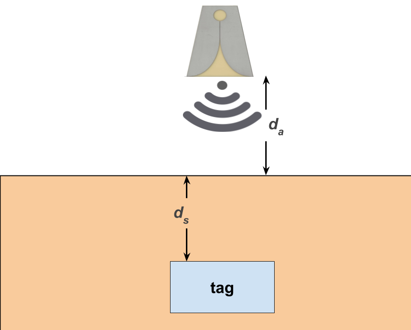
Figure 2. The tag is buried under soil at a known depth $d_{s}$. The radar can measure the ToF/distance between itself and the surface of the ground, $d_{a}$. Using these values, we can calculate $\Delta\tau$, the amount ToF increases due to traveling through soil instead of air

Our key design insight is that we can make soil moisture sensing orders of magnitude more affordable by using a system model similar to RFID: cheap tags paired with a more expensive reader. Using a GPR as the reader is possible, but these devices are often not small enough to be hand-held or mounted on a drone. Instead, we look to consumer-grade radars. Consumer-grade radar systems are becoming increasingly affordable and accessible, which introduces exciting new sensing possibilities. There are multiple radar devices on the market as cheap as $50-400, and modern smartphones have even started integrating them (Lien et al., 2016). In addition to being affordable, these radars tend to be lightweight and portable/handheld.

Consumer-grade UWB radars have the ability to accurately measure the ToF of reflected signals, since their high bandwidth corresponds to a time resolution of 0.15-0.5ns. For comparison, agricultural TDR sensors range from 100Mhz to 3Ghz (Pelletier et al., 2012) which leads to a resolution of at most 0.33ns. Therefore an appropriate selection of UWB radar will allow us to measure ToF with the same accuracy as TDR soil sensors.

Accurate measurement of ToF is not alone sufficient for measuring soil moisture, though. A reference point buried a known distance beneath the soil is required. One work used a large metallic object object underground (Shamir et al., 2018). We realized that versus a plain piece of metal, using a grounded wideband directional antenna would significantly increase the SNR of the signal returning to the radar. This allows us to deploy the reference points deeper, and collect the measurements with inexpensive consumer-grade radars. These radars also have a higher center frequency than GPRs, which allows for smaller antennas and increased portability.

At mass production, these radar backscatter tags would cost similarly to underground RFID tags that municipalities use for utility marking, which cost $5-10 in bulk. The cost to densely outfit a large farm with tags and a few radars would be less then $100,000, which is under a tenth the cost of using traditional soil sensors. Like traditional sensors, the tags would be re-usable across growing seasons. Furthermore, if the tag is buried sufficiently deep it could even remain in the ground if the field is cultivated/tilled, which disturbs the top 15-30cm of soil (Service, 2010).

For a smaller farm, 1-2 acres, taking measurements by hand is feasible. The reader could even be integrated with a mobile phone, which would significantly facilitate adoption in developing nations. For larger farms, taking readings by hand may not scalable, so we assume that the reader would be mounted to a tractor, or possibly an agricultural robot (Aroca et al., 2018) or drone (Vasisht et al., 2017), which are becoming increasingly popular.

In the following sections we expand on the design details behind our system.

3.1. Radar considerations

A modern radar operates using frames, which is the set of samples from a single sweep across the radar’s sensing area. For example, a radar could sweep everything in front of it that lies greater than 1 meter but less than 2 meters away. The sensing area is typically adjustable. The shape of the sensing area depends on the number and type of antennas. We use a pair (one TX, one RX) of directional antennas, as the area of interest lies straight down.

For a pulsed radar, a frame typically has one complex sample per range bin. Each range bin corresponds to a range of possible distances from the radar. For example, if the radar range resolution is 5cm, the magnitude of the sample from the 10th range bin would correspond to an object that is 45-50cm away from the radar. The number and size of range bins depends on both the bandwidth and sensing area. The wider the bandwidth, the smaller the range bins can be. The larger the sensing area, the larger the range bins will be. The size of the range bin determines the ToF resolution as well.

Three key specifications driving our choice of radar are the bandwidth, frame rate. and center frequency. As discussed earlier, any UWB radar with a sufficiently wide bandwidth will provide suitable ToF resolution. All of the radars we considered had a bandwidth of 3 or more Ghz.

The frame rate determines how fast the radar can sweep the sensing area. A faster frame rate means that measurements can be taken more quickly and/or at a higher SNR. A number of radar settings impact the achievable frame rate, including the sensing area and ADC/DAC levels. All three of the radars we tested achieved a frame rate of at least 200fps. For moisture levels typically seen on farms, this allows us to take measurements within 10s for a tag buried at a depth of 30cm.

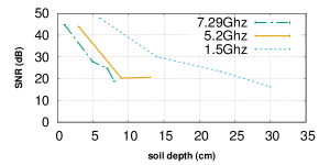
Figure 3. SNR vs soil depth for three radar center frequencies

The center frequency determines how deep beneath the ground a radar can penetrate with a given transmission power. As the wavelength of the RF decreases, the wave attenuates faster due to obstacles and water (see Fig. 3). We ultimately selected the radar centered at 1.5Ghz (a Novelda X1) due to its ability to penetrate soil.

3.2. Backscatter tag

RF backscatter is the principle behind radar, but it has also long been used as a low-power communication technique. RFID, for example, uses an antenna as a reflector and changes the impedance to modulate information on top of the reflected RF. The simplest kind of modulation is binary on-off keying, which toggles the antenna between grounded and open.

By using backscatter to communicate, instead of an active radio chain, these backscatter tags use orders of magnitude less power than traditional radios. Since we are burying our tag underground, long battery life is a primary design goal. Backscatter tags can be passive, semi-passive or active. Passive tags, such as those in anti-theft stickers or door security badges, both harvest their operating power via RF and communicate using backscatter. This depends on having an incoming source of RF with a strong enough signal to enable power harvesting. Semi-passive tags such as (Zhang et al., 2017) use a battery instead of harvesting RF power. Active tags are used in long-distance scenarios, such as toll transponders. These tags both use a battery and amplify the outgoing backscatter reflection. They do not have a full radio chain so they still rely on incoming RF to communicate.

There are no off-the-shelf backscatter tags designed for radar, so we built our own prototype (see Fig 6). UWB radars transmit at low power to avoid causing interference, so passive tags are not an option because the incoming RF is far too quiet for power harvesting. Instead, we implemented semi-passive and active designs. The semi-passive tag has a very simple design, consisting of a UWB Vivaldi antenna, an RF switch and an oscillator. A waterproof case creates an air pocket around the antenna, which acts as a radome and ensures proper impedance matching, as direct contact with soil could cause a mismatch. One might wonder why we need anything beyond an antenna—is the strong reflection not enough? In open air, the answer is yes. Underground, though, the tag is just one reflector among many, many other reflective particles of dirt and rock. We also want a way to isolate reflections that are coming from the tag.

3.2.1. Identifying the tag among dense reflectors

Recall that radars are used to measure speed as well as distance. Our key insight behind how we isolate the signal from the tag leverages the fact that the environment the tag lies within is very stable. Roots grow and water seeps, but at slow speeds. If we make the tag seem like it is moving quickly, the signal will stand out strongly against an effectively stationary backdrop.

Let the impulse the radar transmits be represented by $p(t)$, and the received signal by $r(t)$. Then, the digitized sample for the $n$th range bin can be written as

(11) $$r[n]=\alpha p(nT-\tau)$$

where $T$ is the sampling period, $\alpha$ is the complex attenuation and $d_{k}$ is the distance of the range bin in meters. Time of flight, $\tau_{k}=2d_{k}/c$, is the time for a radar impulse to travel to an object and then reflect back again.

Above, for simplicity we have assumed that there is only one reflector per range bin, but in reality there are multiple reflections in a range bin since dirt is small and dense. Taking that into account, the resulting sample will then become be the linear combination of all $k$ reflectors in the same bin:

(12) $$r[n]=\sum\limits_{k=1}^{K}\alpha_{k}p(nT-\tau_{k})$$

Because pulse-based radars transmit at a regular interval known as the pulse repetition interval (PRI), they can be used to obtain the speed of moving objects. If an object is moving at a constant speed of $v$ m/s, then every frame the object’s ToF changes by $2v\Delta/c$ where $\Delta$ is the PRI.

This change in the time-domain corresponds to a phase change in the frequency domain: $\phi_{k}=2\pi f(2v_{k}\Delta/c)$. Although the phase changes for each frequency within the bandwidth of the impulse, we can simplify the math by using only the radar’s center frequency $f_{c}$. Then, the value for the $n$th bin in the $m$th frame will be

(13) $$r_{m}[n]=\sum\limits_{k=1}^{K}\alpha_{k}p(nT-\tau_{k})e^{-j2\pi\frac{2v_{k}\Delta(m-1)}{\lambda}}$$

where $\lambda$ is the wavelength of the radar center frequency, $f_{c}$.

Note how similar Eq. 13 is to the discrete Fourier transform:

(14) $$F_{k}=\sum\limits_{k=1}^{N-1}f_{n}e^{\frac{-j2\pi}{N}kn}$$

If we apply a 1-D inverse Fourier transform to each range bin across a collection of P pulses, we get a range-Doppler image which tells us the speed of moving objects:

(15) $$R[n,s]=\frac{1}{P}\sum\limits_{i=1}^{P}r_{m}[n]e^{j2\pi\frac{(i-1)(s-1)}{P+1}}$$

In Eq. 15 above, $s$ is the Doppler bin and $n$ is the range bin and $P$ is the total number of pulses transmitted over the collection time.

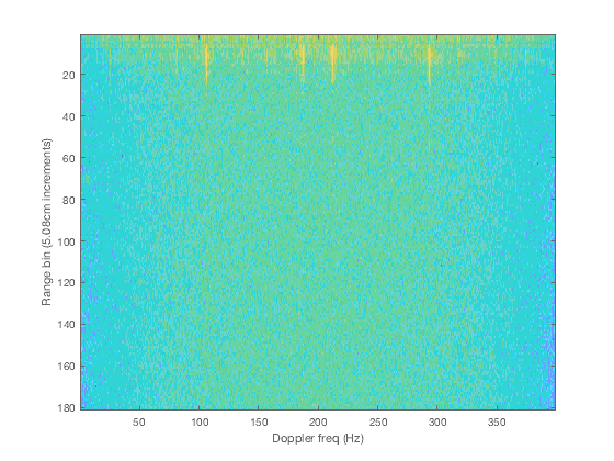
Figure 4. Range-Doppler image generated from a 10s radar capture. The bright spots at 212 and 293 Hz correspond to the oscillation of an antenna that is grounded and ungrounded at 212 Hz. The additional frequencies are harmonics caused by the square-wave nature of the tag pattern.

Figure 4 shows an example range-Doppler plot. We can see that there are bright spots at 212 and 293 Hz. This plot is a 10 second capture where the radar is pointed at an antenna that is grounded and ungrounded at 212 Hz.If there are no other fast-moving objects in the radar’s field of view, and the frame rate of the radar is sufficiently high, we can use this property to discern the signal from our backscatter tag from the signals due to other reflectors.

Ultimately we set our tag to oscillate at 80Hz, which is below the Nyquist frequency of our 200fps frame rate, but between the 60 and 120Hz interference caused by AC power.

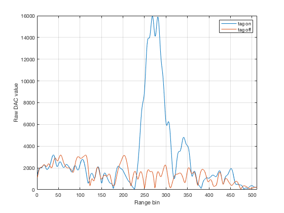
Figure 5. Plot of the range-Doppler vector corresponding to 80Hz, the frequency our tag oscillates at. When the tag is on, we see a very strong peak compared to when the tag is off

Figure  5 shows the plot of the vector corresponding to the 80Hz frequency bin in our range-Doppler matrix. A strong peak appears in bin 268 only when the tag is on. Thus we’ve successfully identified the signal from the tag. This approach has the additional advantage the SNR of the signal of the tag increases with integration time. That is, the more frames we capture, the better the signals gets. So if a capture yields an ambiguous peak, we can simply capture additional frames.

3.2.2. Amplification

A semi-passive tag works well in typical soil conditions, but for tags in especially deep and/or wet soil, the tag signal is too weak to reliably detect. Therefore we also designed an active variant of our tag that adds an amplifier. The incoming RF is amplified before going into the RF switch, which has another antenna attached to it. The oscillator causes this second antenna to toggle on and off with the amplified signal, allowing the tag to operate in more extreme conditions. This active tag is completely indistinguishable to the radar receiver, so we can use the same procedure to measure soil moisture for both tags.

3.3. Putting it all together

This system relies on the user knowing a.) where the tag is located in the field and b.) how deep the tag is buried. With this information we know $d_{s}$, the amount of soil the direct path of RF has to travel through (Fig. 2). A few simple options make tracking this data easy, such as using marking flags, annotated GPS coordinates, or slightly changing the oscillation frequency of each tag allowing for a lookup table that maps between frequency and tag depth/location. Taking measurements with the radar not located directly over the tag does add error. Using directional antennas in both the tag and radar helps minimize the chances of taking measurements off-center, since the signal strength will be much weaker when the radar isn’t directly overhead. Another option is using a more sophisticated radar with multiple receive antennas, which would enable adjusting $d_{s}$ with angle of arrival data.

Another piece of information is still needed to measure soil moisture: the distance between the radar and the surface of the ground, $d_{a}$. The radar itself can easily measure this. In our experiments, $d_{a}$ ranged between 0.5-2m.

Then, using the technique outlined in 3.2.1, our system finds the range bin of the backscatter tag, $b_{r}$. The expected range bin if there were no dirt on top of the tag is $b_{T}=d_{a}/r+d_{s}/r$, where $r$ is the range resolution of the radar.

Now we can calculate $\Delta\tau$, the change in ToF caused by the soil:

(16) $$\Delta\tau=\frac{(b_{r}-b_{T})r}{c}$$

The approximate apparent dielectric constant of the soil is

(17) $$K_{a}\approx\left(\frac{c\Delta\tau}{d}\right)^{2}$$

Finally, this apparent permittivity is fed directly into a known equation like the Topp equation to determine VWC.

4. Implementation

Table 1. Always-on power consumption of prototypes

	Oscillator	RF switch	Power management	RF detector	Amplifier	MCU	TOTAL
Active tag	2.7uW	63uW	51uW	87mW (3uW shutdown)	267mW	378uW (2.2uW)	354.495mW
Semi-passive tag	2.7uW	63uW	51uW	—	—	—	0.116mW

The radar chip we used was the X1 (NVA6100) by Novelda, which is centered at 1.5Ghz and has a bandwidth of 3Ghz. The chip is $100 per unit. We interface with the radar via a development kit made by Flat Earth Inc (Inc., [n. d.]) that runs on a BeagleBone Black single-board computer. For these evaluations the radar captures were processed via MATLAB, but the signal processing required could relatively easily be ported to run in a low-level language on on a BeagleBone or smartphone. All of our source code will be released to ensure reproducibility.

The backscatter tags have three primary components: an SiT1534 programmable oscillator, an HMC1118 RF switch and a Vivaldi ultra-wideband antenna (see Fig. 6). A TPS76933 voltage regulator manages power when the tag is powered by battery. The active tag has an additional antenna and an HMC374 amplifier.

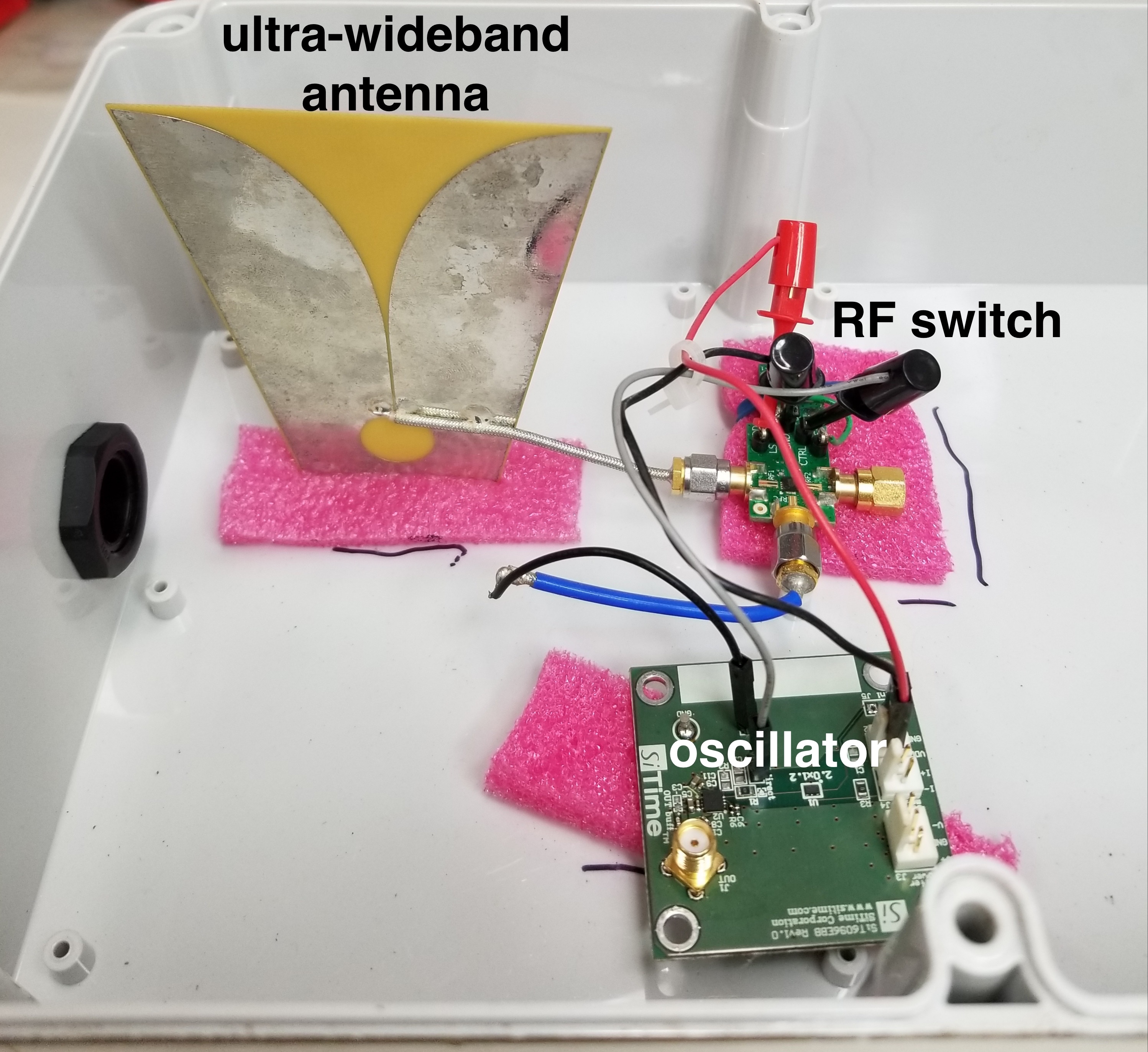
Figure 6. Prototype of a semi-passive tag

4.1. Power consumption

The primary area of concern with regards to power consumption is the backscatter tag, since it is underground and the batteries cannot be easily replaced. The power consumption of the radar is still important, especially if the readings will be collected via drone, but we assume that the radar reader system can be charged at least daily. The NVA6100 radar chip we use consumes 116mW of power (Inc, 2010), and the entire reader system (radar chip plus BeagleBone Black board) consumes 450mW, about a quarter of what smartphones consume. Power consumption could be further reduced in the future by using a low-power microcontroller platform (e.g. MSP430) instead of a BeagleBone Black.

The power consumption for both the active and semi-passive tags is presented in Table 1. The battery lifetime of the semi-passive sensor is projected to be 15.02 years on 4$\times$AA batteries rated for 2500mAh. The active sensor consumes an order of magnitude more power, so without duty cycling the battery life would be about two months. However, using an RF detector such as the LT5538 that is powered up once per second to check for a wake signal, the battery lifetime could be 3-4 years. This comes at the cost of a more complicated system—the transmit power of UWB radar is required to be very low by federal regulation in most countries, which makes it insufficient for providing a wake signal. However, since the tag antenna is wideband, a narrowband signal such as WiFi or RFID can be used to wake up the tag instead. Narrowband signals can be transmitted at powers up to 4W when a directional antenna is used. Using a VNA we measured the attenuation of an omnidirectional wake signal centered at 2.4Ghz, and found that travelling through 30cm of fully-saturated clay loam causes losses of about 80-90dB. A 30-36dB transmission would be high enough power to overcome that and successfully activate many RF detectors.

Unless the tag needs to be deployed in adverse conditions where the soil is extremely wet and/or has high clay content, the active sensor is probably not worth the added complication and decreased battery life.

5. Evaluation

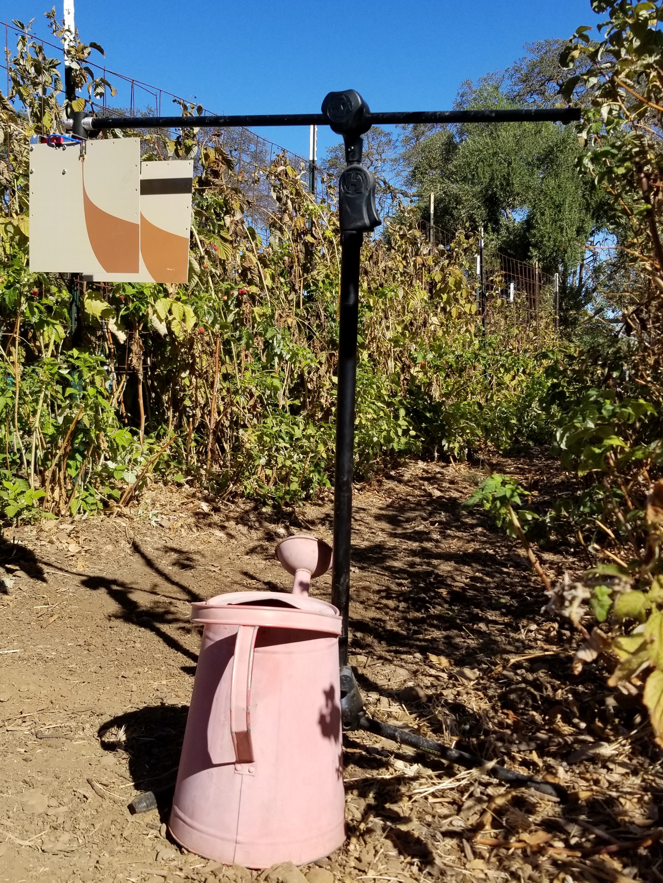
Figure 12. Setup for in situ experiments at a local farm. The radar is pointed at an underground tag, and the surface of the soil is watered in 7L increments using a watering can.

We evaluate our system in both laboratory and in situ settings. The laboratory evaluations were done using a large bin containing about a cubic meter of soil to ensure that the backscatter tag is covered equally by soil on all sides. The in situ evaluations were done at a local organic farm whose fields contain sandy silt loam soil (see Fig. 12). We used the same local tap water for all experiments. Below we discuss experimental considerations in more detail.

5.1. Soil type selection

Soil can be broadly classified into three main types: clay, sand and silt. Soils that are purely one type are rare, however, and most are a mixture of two or more types (see Fig. 7). Loam is a roughly even combination of clay, silt and sand. Loamy soils are considered to be ideal for agriculture (Parikh and James, 2012), and most crops are grown in soil that lies within the loam spectrum. We test on three sub-types of loam: sandy clay loam, silt loam and clay loam. Testing a variety of soils is important because the soil type can strongly impact RF propagation properties. For example, clay soils have fine particle that allow it to hold water very well, and they also tend to high higher organic matter content which impacts the electrical conductivity (EC), which makes it more difficult for RF to penetrate.

We collected our soils by consulting a recent map of farmland soil classifications (Santa Clara County, 2015). All three soils are identified by the USDA as suitable for agriculture.

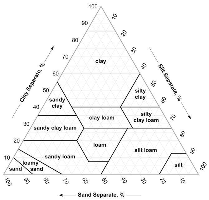
Figure 7. Soil textural triangle (USDA, [n. d.])

5.2. Electrical conductivity

As mentioned earlier, the depth that RF of a given wavelength can penetrate into the ground (skin/penetration depth) is heavily impacted by the soil’s moisture content (which dictates the permittivity) and also the EC.

Increasing water content increases both the permittivity and EC. Soil with high organic matter content sees a greater increase in EC when water is added. For example, our measurements found that the EC of fully-saturated potting soil is 10x that of fully-saturated sandy clay loam. It still works in potting soil, but the maximum reliable deployment depth is only 10-15cm vs the up to 75cm possible with loam soils typically seen on farms.

Furthermore, soil amendments such as compost or liquid fertilizer can also increase the EC of soil. Most farms maintain an EC between 0.75-2mS/cm (Instruments, [n. d.]). In our experiments the EC remained within that range for all soils except potting soil. Fortunately, we did not see significant RF attenuation until EC levels rose above 2mS/cm.

5.3. Root zone depth

Root zone depth, or maximum root zone depth, is the maximum depth of a plant’s roots. The effective root zone depth is the depth of soil that a plant’s roots extract the most moisture. About 70% of the moisture extracted by a plant’s roots is from the top half of the maximum root zone. For example, celery has a maximum root depth of 60cm, and an effective root zone depth of 30cm. This means that moisture should be monitored within the top foot of soil.

Most crops have an effective root depth between 15-60cm, however fruit crops (especially those that grow on trees) can extend as deep as 75cm (USDA, 1997). Our laboratory experiments were done at a depth of 30cm primarily due to the limitations of container sizes that could ensure the sensor was covered on all sides, but our in situ experiments (see Fig. 14) suggest that it could be deployed at depths up 75cm.

5.4. Calibration

All soil moisture sensors require a one-time soil-specific calibration to achieve high accuracy. One common calibration procedure is gravimetric, which involves weighing wet samples, oven drying them to calculate the ground-truth VWC, and then fitting those measurements to the sensor readings that were taken at the time of sample collections to produce a custom equation that relates sensor output to VWC. We performed gravimetric calibrations for both our commercial sensor and radar sensor.

If lower accuracy is acceptable, soil-specific calibration is not necessary and a general equation like the Topp equation can be used instead.

Unlike other RF-based solutions such as (Ding and Chandra, 2019) (Aroca et al., 2018), our system does not require any additional calibration as compared to commercial soil sensors. However, accurate records of the depth the sensor was deployed at are required. This depth can be measured manually, or by using the radar itself once the sensor is placed in the hole (but before the soil is replaced). We use the latter approach in our evaluations.

6. Results

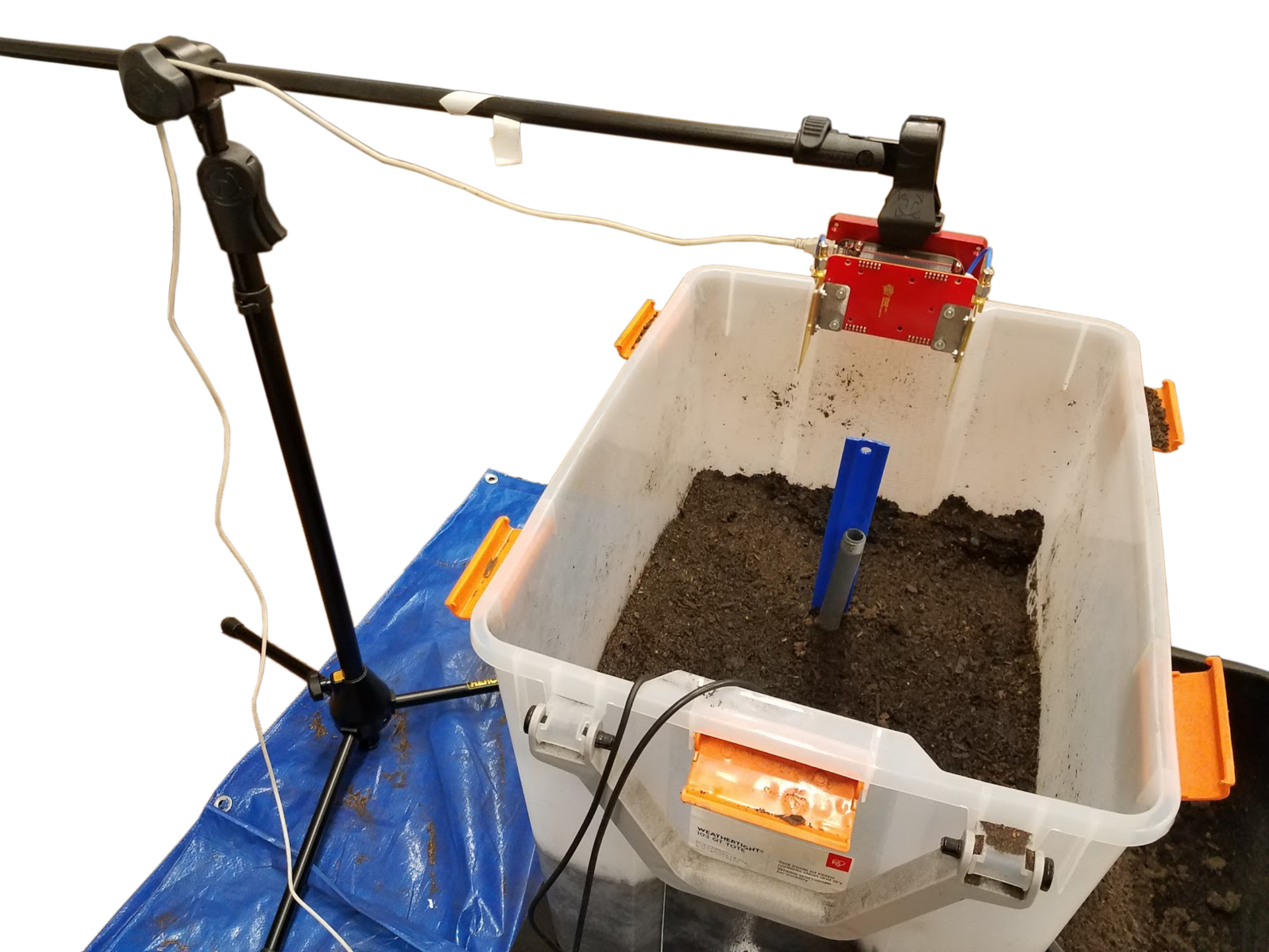
Figure 8. Setup for laboratory experiments

6.1. Laboratory

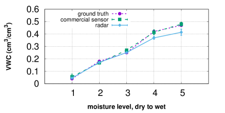
(a) Sandy clay loam

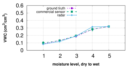
(b) Silt loam

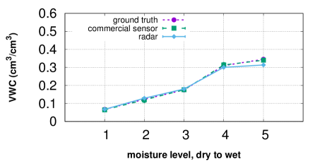
(c) Clay loam

Figure 9. Active tag VWC measurements of three soil types from dry to saturated with the tag buried at a depth of 30cm. Moisture level 1 is completely dry soil which was then gradually dampened in 7 liter increments until saturation at level 5. Note that saturation depends on the soil type.

Figure 9 shows the results from our active tag. Each radar datapoint is the average and standard deviation of 10 measurements. The radar captures used for the measurements lasted 10-30s with the exception of the saturation moisture levels which used 100s captures. Each commercial sensor datapoint is the average and standard deviation of 3-5 measurements, where each measurement is taken in a different part of the soil. The size of the container we conducted experiments in limited the number of commercial sensor datapoints. To conduct the experiment, we began with about a cubic meter air-dried soil and gradually dampened in 7 liter increments. In these laboratory experiments we homogenized the soil moisture by mixing the added water vigorously by hand. This was to ensure that the Teros 12 sensor we compared against was not biased by wet or dry pockets of soil.

We see that for all soil types both our system and the commercial sensor closely track the ground truth, which is the average of two oven-based volumetric measurements per moisture level. The average error of our system is $0.015cm^{3}/cm^{3}$, compared to $0.007cm^{3}/cm^{3}$ on the commercial Teros 12 sensor. Though our system’ss average error is higher than the commercial sensor, it is not significant. Calibrated commercial sensors are advertised having an average error between $0.01-0.03cm^{3}/cm^{3}$. The greatest error is seen with the sandy clay loam soil at saturation, where our system underestimates VWC by $0.05cm^{3}/cm^{3}$. This maximum level of error is also typical among commercial sensors.

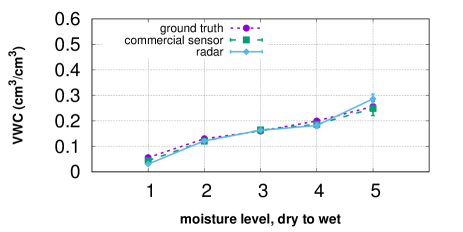
(a) Sandy clay loam

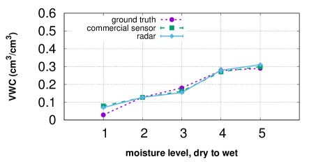
(b) Silt loam

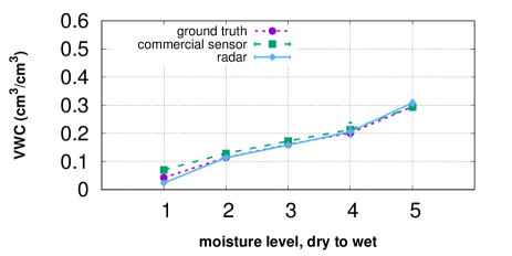
(c) Clay loam

Figure 10. Passive tag VWC measurements of three soil types from dry to loss of signal with the tag at a depth of 30cm. Moisture level 1 is completely dry soil which was then gradually dampened in 4-5 liter increments.

Figure 9 shows the results from our passive tag. This time we added water in $4-5L$ increments and stopped when the signal from the passive tag was no longer visible. This was typically 5-15% before saturation. Again, both our system and the commercial sensor closely track the ground truth, with our system achieving an average error of $0.014cm^{3}/cm^{3}$ and the commercial sensor $0.013cm^{3}/cm^{3}$. The maximum error for both our system and the commercial sensor was $0.04cm^{3}/cm^{3}$.

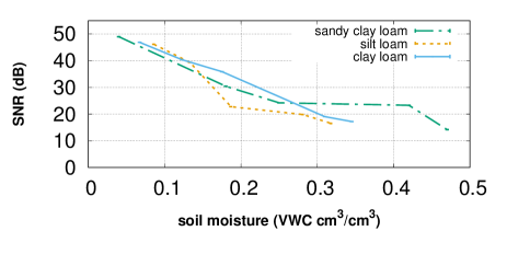
(a) Active tag

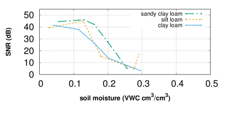
(b) Passive tag

Figure 11. SNR vs VWC of 100s captures for passive and active tags in the laboratory

Figure 11 shows the results of SNR vs soil moisture for both tags across the three different soil types. As expected, the SNR for the passive tag decreases more quickly than the active tag as moisture level increases. Also, the signal in both silt and clay loam soils is weaker than the sandy clay loam. There does not appear to be a significant difference between silt and clay loams, though.

6.2. In situ

Figure 13 shows the results of both passive and active tags for the in situ VWC experiments. In these experiments our tag was buried under 30cm of soil. For comparison, we used two Teros 12 sensors, one at a depth of 30cm and the other near the surface at a depth of 5cm. Unlike the laboratory experiments, we do not disturb the soil and instead let the water seep over time. The deeper commercial sensor showed no change in soil moisture across the experiments, even after applying more than 20 liters of water and letting it seep overnight. Water did successfully seep into the soil around the shallow sensor, but there was still a delay of up to an hour between watering and seeing the change of moisture level.

As expected, since our system measures the average moisture of the soil between the tag and the surface, it closely tracks the average of the two Teros sensors. Furthermore, our system reacts immediately to the addition of water. This suggests that it provides faster feedback after water application than traditional sensors, which might prevent over-watering. Furthermore, it inherently reflects the average soil moisture across the whole effective root zone, whereas multiple commercial sensors are required to accomplish the same.

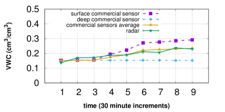
(a) Active tag

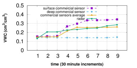
(b) Passive tag

Figure 13. VWC in situ on a farm field with passive and active tags buried at a depth of 30cm. Measurements were taken every 30 minutes, with 7 liters of water poured on the soil at times 2, 4, 6 and 8.

One of the limitations of our laboratory experiments is that it is difficult to evaluate with the tag buried more than 30 cm deep, since covering the tag with $>$30cm of dirt on all sides would require bringing a prohibitively large amount of dirt indoors. Outdoors, we were able to dig a hole more than 75cm deep and gradually cover the tag with dirt. Fig. 14 shows the results of these experiments. At a VWC of $0.15cm^{3}/cm^{3}$ we were still able to detect both tags successfully at a depth of 77cm. This suggests that it can probably be deployed deeper than the 30cm evaluated in-laboratory to accurately measure the VWC typically seen on farms.

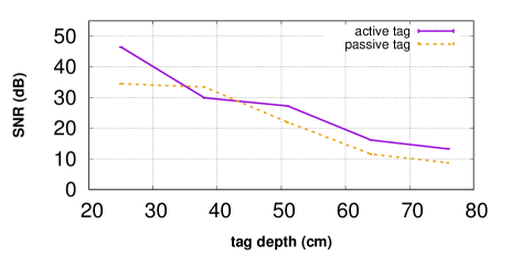
Figure 14. SNR vs tag depth of 100s captures for passive and active tags. Measurements were performed in an actively watered farm field containing sandy clay loam. The VWC of the soil was about 15% at the time of measurement.

Figure 15 shows how the SNR for both active and passive tags changes with VWC. Compared to the laboratory experiments (Fig 11), the passive tag SNR drops off much less steeply. This further suggests that the passive version of the tag is well-suited for agriculture and that the added complication and reduced battery life of the active tag will usually not be necessary.

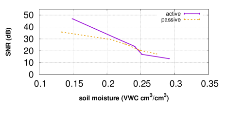
Figure 15. SNR vs VWC in situ for 100s captures on a farm field with passive and active tags buried at a depth of 30cm

7. Related Work

In addition to GPR techniques, other works have also used RF to measure soil moisture. Strobe (Ding and Chandra, 2019) uses commodity WiFi transmissions to measure relative ToF between buried antennas. These antennas require being wired to a power-hungry 802.11 WiFi chip. Furthermore, there are significant additional calibration procedures required. Non-radar UWB transceivers have also used ToF to perform sensing such as localizaton (Gro$\beta$windhager et al., 2019) and ECG (Toll, 2019).

Researchers in Israel used ToF measured via a $20,000 GPR paired with buried metal bars (Shamir et al., 2018) to measure soil moisture. The radar used requires direct contact with the surface of the soil, though, and the accuracy to our system is similar.

Our system is inspired by RFID, which has itself been used to classify food and beverages (Ha et al., 2018) (Wang et al., 2017) and measure soil moisture (Aroca et al., 2018). The latter work uses commodity RFID tags paired with neural networks to determine soil moisture via RSSI. This work has the drawback that the neural network has to be re-trained for every single soil type and deployment depth. However, they have successfully gotten an agricultural robot to collect the moisture measurements autonomously.

8. Discussion and Conclusion

We believe our system has the potential to be useful to farmers with both large and small farms. There are a number of steps between this work and real-world deployment, however.

The environmental impact of the tags needs to be considered. Wireless tags are more easily lost. Research into biodegradable printed circuit boards (Guna et al., 2016) and soil batteries (Lin et al., 2015) may allow for a more eco-friendly version that doesn’t leach harmful elements into the soil over time.

We acknowledge that there is a lot of engineering and political work to go from laboratory prototype to field trials, especially trials in developing nations. We hope to trial our system at local farms soon, and someday at farms in developing nations.

We also realize that there is a lot of active research in how to best utilize agricultural robots and drones. These technologies have seen some adoption, but in general much research remains for determining how to scale.

There are also a number of additional research opportunities we would like to explore:

1. Creating a tag with two antennas/oscillators would allow us to relative ToF in addition to absolute. Our system currently measures absolute ToF, which corresponds to average soil moisture, but sometimes point soil moisture is preferred. Furthermore it can be calculated without knowledge of the tag deployment depth if the separation between antennas is known.

2. Encoding additional information into radar backscatter so that the tag itself can store information like deployment depth and location, eliminating the need for the operator to use a lookup system.

3. Sensing opportunities beyond soil moisture such as measuring EC and contaminant mapping.

9. Summary

In this paper we presented a two-part system for sensing soil moisture with RF that combines low-cost backscatter tags with a consumer-grade UWB radar acting as a reader. We achieve completely wireless soil moisture sensing with an accuracy comparable to that of state-of-the-art commercial and scientific sensors at an order of magnitude lower cost. We acknowledge that there is a large gap between small-scale prototype and systems deployed at scale, but we believe that it has the potential to become an effective soil sensing solution for farmers in both developing and developed nations.

References

- (1)
- Agency (2013) United States Envrionmental Protection Agency. 2013. WaterSense Notice of Intent (NOI) to Develop a Draft Specification for Soil Moisture-Based Control Technologies. https://www.epa.gov/sites/production/files/2017-01/documents/ws-products-noi-sms.pdf.
- Aquastat (2014) Aquastat. 2014. Water withdrawal by sector. http://www.globalagriculture.org/fileadmin/files/weltagrarbericht/AquastatWithdrawal2014.pdf.
- Aroca et al. (2018) Rafael V. Aroca, André C. Hernandes, Daniel V. Magalhães, Marcelo Becker, Carlos Manoel Pedro Vaz, and Adonai G. Calbo. 2018. Calibration of Passive UHF RFID Tags Using Neural Networks to Measure Soil Moisture. Journal of Sensors 2018 (2018), 1–12. https://doi.org/10.1155/2018/3436503
- Azevedo and McEwan (1997) S. Azevedo and T.E. McEwan. 1997. Micropower impulse radar. IEEE Potentials 16, 2 (apr 1997), 15–20. https://doi.org/10.1109/45.580443
- Balasubramanian (2016) Vethaiya Balasubramanian. 2016. How many soil moisture sensors are required for 20 acres land? https://www.quora.com/How-many-soil-moisture-sensors-are-required-for-20-acres-land.
- Datta et al. (2018) Sumon Datta, Saleh Taghvaeian, Tyson Ochsner, Daniel Moriasi, Prasanna Gowda, and Jean Steiner. 2018. Performance Assessment of Five Different Soil Moisture Sensors under Irrigated Field Conditions in Oklahoma. Sensors 18, 11 (nov 2018), 3786. https://doi.org/10.3390/s18113786
- Ding and Chandra (2019) Jian Ding and Ranveer Chandra. 2019. Towards Low Cost Soil Sensing Using Wi-Fi. In The 25th Annual International Conference on Mobile Computing and Networking - MobiCom '19. ACM Press. https://doi.org/10.1145/3300061.3345440
- Fares et al. (2013) Ali Fares, Marouane Temimi, Kelly Morgan, and Thijs J. Kelleners. 2013. In-Situ and Remote Soil Moisture Sensing Technologies for Vadose Zone Hydrology. Vadose Zone Journal 12, 2 (2013), 0. https://doi.org/10.2136/vzj2013.03.0058
- Greenlee (2019) Greenlee. 2019. OmniMarker. https://www.greenleestore.com/products/greenlee-0162-0001-1-omni-marker-green.
- Growindhager et al. (2019) Bernhard Growindhager, Michael Stocker, Michael Rath, Carlo Alberto Boano, and Kay Römer. 2019. SnapLoc: an ultra-fast UWB-based indoor localization system for an unlimited number of tags. In 2019 18th ACM/IEEE International Conference on Information Processing in Sensor Networks (IPSN). IEEE, 61–72.
- Guna et al. (2016) Vijay Kumar Guna, Geethapriya Murugesan, Bhuvaneswari Hulikal Basavarajaiah, Manikandan Ilangovan, Sharon Olivera, Venkatesh Krishna, and Narendra Reddy. 2016. Plant-Based Completely Biodegradable Printed Circuit Boards. IEEE Transactions on Electron Devices 63, 12 (dec 2016), 4893–4898. https://doi.org/10.1109/ted.2016.2619983
- Ha et al. (2018) Unsoo Ha, Yunfei Ma, Zexuan Zhong, Tzu-Ming Hsu, and Fadel Adib. 2018. Learning Food Quality and Safety from Wireless Stickers. In Proceedings of the 17th ACM Workshop on Hot Topics in Networks - HotNets '18. ACM Press. https://doi.org/10.1145/3286062.3286078
- Hrozencik (2019) Aaron Hrozencik. 2019. Irrigation & Water Use. United States Department of Agriculture Economic Research Service (2019).
- Hussain (1998) Malek GM Hussain. 1998. Ultra-wideband impulse radar-an overview of the principles. IEEE Aerospace and Electronic Systems Magazine 13, 9 (1998), 9–14.
- Inc. ([n. d.]) FlatEarth Inc. [n. d.]. Chipotle Radar Development Kit AVA 0.8 - 4 GHz. https://store.flatearthinc.com/collections/chips-salsa/products/chipotle-radar-development-kit.
- Inc (2010) Novelda Inc. 2010. NVA6100 Datasheet.
- Instruments ([n. d.]) Miluakee Instruments. [n. d.]. AG900 Manual. http://www.milwaukeeinstruments.com/site/pdf/Master_AG900_Manual.pdf.
- International (2014) ICT International. 2014. Which soil moisture sensor should I choose? http://www.ictinternational.com/case-study-pdf/?product_id=1483.
- Jol (2008) Harry Jol. 2008. Ground Penetrating Radar Theory and Applications. Elsevier Science.
- Li et al. (2016) Wenda Li, Bo Tan, and Robert J. Piechocki. 2016. Non-contact breathing detection using passive radar. In 2016 IEEE International Conference on Communications (ICC). IEEE. https://doi.org/10.1109/icc.2016.7511389
- Lien et al. (2016) Jaime Lien, Nicholas Gillian, M. Emre Karagozler, Patrick Amihood, Carsten Schwesig, Erik Olson, Hakim Raja, and Ivan Poupyrev. 2016. Soli. ACM Transactions on Graphics 35, 4 (jul 2016), 1–19. https://doi.org/10.1145/2897824.2925953
- Lin et al. (2015) Fu-To Lin, Yu-Chun Kuo, Jen-Chien Hsieh, Hsi-Yuan Tsai, Yu-Te Liao, and Huang-Chen Lee. 2015. A Self-Powering Wireless Environment Monitoring System Using Soil Energy. IEEE Sensors Journal 15, 7 (jul 2015), 3751–3758. https://doi.org/10.1109/jsen.2015.2398845
- McClellan (2018) Tai McClellan. 2018. Soil composition. University of Hawai‘i – College of Tropical Agriculture and Human Resources. https://www.ctahr.hawaii.edu/mauisoil/a_comp.aspx.
- Noborio (2001) K. Noborio. 2001. Measurement of soil water content and electrical conductivity by time domain reflectometry: a review. Computers and Electronics in Agriculture (2001). https://eurekamag.com/pdf/003/003495928.pdf.
- of Economic and Social Affairs (2017) United Nations Department of Economic and Social Affairs. 2017. World Population Prospects: The 2017 Revision, Key Findings and Advance Tables. https://population.un.org/wpp/Publications/Files/WPP2017_KeyFindings.pdf.
- Parikh and James (2012) Sanjai J. Parikh and Bruce R. James. 2012. Soil: The Foundation of Agriculture. Nature Education Knowledge (2012).
- Patitz et al. (1995) Ward E Patitz, Billy C Brock, and Edward G Powell. 1995. Measurement of dielectric and magnetic properties of soil. Technical Report. Sandia National Labs.
- Pelletier et al. (2012) Mathew G. Pelletier, Sundar Karthikeyan, Timothy R. Green, Robert C. Schwartz, John D. Wanjura, and Greg A. Holt. 2012. Soil Moisture Sensing via Swept Frequency Based Microwave Sensors. Sensors 12, 1 (jan 2012), 753–767. https://doi.org/10.3390/s120100753
- Raza et al. (2016) Usman Raza, Parag Kulkarni, and Mahesh Sooriyabandara. 2016. Low Power Wide Area Networks: A Survey. CoRR abs/1606.07360 (2016). arXiv:1606.07360 http://arxiv.org/abs/1606.07360
- Richards (2010) Mark A. Richards. 2010. Principles of Modern Radar. INSTITUTION ENGINEERING & TECH. https://www.ebook.de/de/product/11344959/mark_a_richards_principles_of_modern_radar.html
- Santa Clara County (2015) Planning Office Santa Clara County, CA. 2015. Farmland Classification of Soils: Santa Clara County, California. http://purl.stanford.edu/mp959nm6914.
- Schimmelpfennig (2016) David Schimmelpfennig. 2016. Farm Profits and Adoption of Precision Agriculture. Economic Research Service/USDA (2016).
- Service (2010) USDA Natural Resources Conservation Service. 2010. Tillage Equipment Pocket Identification Guide. https://www.nrcs.usda.gov/Internet/FSE_DOCUMENTS/nrcs142p2_007135.pdf.
- Shamir et al. (2018) Omer Shamir, Naftaly Goldshleger, Uri Basson, and Moshe Reshef. 2018. Laboratory Measurements of Subsurface Spatial Moisture Content by Ground-Penetrating Radar (GPR) Diffraction and Reflection Imaging of Agricultural Soils. Remote Sensing 10, 10 (oct 2018), 1667. https://doi.org/10.3390/rs10101667
- Toll (2019) Maria Toll. 2019. Wireless electrocardiogram based on ultra-wideband communications.
- Topp et al. (1980) G. C. Topp, J. L. Davis, and A. P. Annan. 1980. Electromagnetic determination of soil water content: Measurements in coaxial transmission lines. Water Resources Research 16, 3 (jun 1980), 574–582. https://doi.org/10.1029/wr016i003p00574
- USDA ([n. d.]) USDA. [n. d.]. Soil Textural Triangle. https://www.nrcs.usda.gov/wps/portal/nrcs/detail/soils/edu/kthru6/?cid=nrcs142p2_054311.
- USDA (1997) USDA. 1997. National Engineering Handbook Irrigation Guide.
- USDA (2018) USDA. 2018. Farms and Land in Farms 2017 Summary. http://usda.mannlib.cornell.edu/usda/current/FarmLandIn/FarmLandIn-02-16-2018.pdf.
- Vasisht et al. (2017) Deepak Vasisht, Zerina Kapetanovic, Jong-ho Won, Xinxin Jin, Ranveer Chandra, Ashish Kapoor, Sudipta N. Sinha, Madhusudhan Sudarshan, and Sean Stratman. 2017. Farmbeats: An IoT Platform for Data-driven Agriculture. In Proceedings of the 14th USENIX Conference on Networked Systems Design and Implementation (NSDI’17). USENIX Association, Berkeley, CA, USA, 515–528. http://dl.acm.org/citation.cfm?id=3154630.3154673
- Wang et al. (2017) Ju Wang, Jie Xiong, Xiaojiang Chen, Hongbo Jiang, Rajesh Krishna Balan, and Dingyi Fang. 2017. TagScan. In Proceedings of the 23rd Annual International Conference on Mobile Computing and Networking - MobiCom 17. ACM Press. https://doi.org/10.1145/3117811.3117830
- Ward and Folkesson (2016) Erik Ward and John Folkesson. 2016. Vehicle localization with low cost radar sensors. In 2016 IEEE Intelligent Vehicles Symposium (IV). IEEE. https://doi.org/10.1109/ivs.2016.7535489
- Wu et al. (2019) Kaijun Wu, G Rodriguez, Marjana Zajc, Elodie Jacquemin, Michiels Clément, and Sébastien Lambot. 2019. A New Drone-Borne GPR for Soil Moisture Mapping. In 10th International Workshop on Advanced Ground Penetrating Radar.
- Zhang et al. (2017) Pengyu Zhang, Colleen Josephson, Dinesh Bharadia, and Sachin Katti. 2017. FreeRider. In Proceedings of the 13th International Conference on emerging Networking EXperiments and Technologies - CoNEXT 17. ACM Press. https://doi.org/10.1145/3143361.3143374
- Zotarelli et al. (2009) Lincoln Zotarelli, Johannes M. Scholberg, Michael D. Dukes, Rafael Muñoz-Carpena, and Jason Icerman. 2009. Tomato yield, biomass accumulation, root distribution and irrigation water use efficiency on a sandy soil, as affected by nitrogen rate and irrigation scheduling. Agricultural Water Management 96, 1 (jan 2009), 23–34. https://doi.org/10.1016/j.agwat.2008.06.007