Xiao-Yun Cai, Zhenjiang College, No. 518 Changxiangxi Avenue, College Park, Zhenjiang 212028, China.
A sparsity augmented probabilistic collaborative representation based classification method
Abstract
In order to enhance the performance of image recognition, a sparsity augmented probabilistic collaborative representation based classification (SA-ProCRC) method is presented. The proposed method obtains the dense coefficient through ProCRC, then augments the dense coefficient with a sparse one, and the sparse coefficient is attained by the orthogonal matching pursuit (OMP) algorithm. In contrast to conventional methods which require explicit computation of the reconstruction residuals for each class, the proposed method employs the augmented coefficient and the label matrix of the training samples to classify the test sample. Experimental results indicate that the proposed method can achieve promising results for face and scene images. The source code of our proposed SA-ProCRC is accessible at https://github.com/yinhefeng/SAProCRC.
keywords:
image recognition, probabilistic collaborative representation based classification, sparse representation, sparsity augmented1 Introduction
Image recognition remains one of the hottest topics in the communities of computer vision and pattern recognition. During the past decade, sparse representation has been successfully applied in various domains. In face recognition, the pioneering work is the sparse representation based classification (SRC) Wright (2009). Concretely, SRC employs all the training samples as a dictionary, and a test sample is sparsely coded over the dictionary, then the classification is performed by checking which class yields the least reconstruction error. SRC can achieve promising recognition results even when the test samples are occluded or corrupted. To further promote the robustness of SRC, Wang et al.Wang (2016) proposed a correntropy matching pursuit (CMP) method for robust sparse representation based recognition. CMP can adaptively assign small weights on severely corrupted entries of data and large weights on clean ones, thus reducing the effect of large noise. Wu et al.Wu (2018) presented a gradient direction-based hierarchical adaptive sparse and low-rank (GD-HASLR) algorithm to tackle the real-world occluded face recognition problem. Gao et al.Gao (2017) developed a robust and discriminative low-rank representation (RDLRR) method by exploiting the low-rankness of both the data representation and each occlusion-induced error image simultaneously. Keinert et al.Keinert (2019) designed a group sparse representation-based method for face recognition (GSR-FR) which introduces a non-convex sparsity-inducing penalty and a robust non-convex loss function.
Apart from classifier design, feature extraction is also a crucial stage in image recognition. The most classic subspace learning based approaches are principal component analysis (PCA) and linear discriminant analysis (LDA). Motivated by the recent development of sparse representation, Qiao et al.Qiao (2010) presented a dimensionality reduction technique called sparsity preserving projections (SPP). To make SRC efficiently deal with high-dimensional data, Cui et al.Cui (2018) proposed an integrated optimisation algorithm to implement feature extraction, dictionary learning and classification simultaneously. To tackle the corrupted data, Xie et al.Xie (2018) explored a dimensionality reduction method termed low-rank sparse preserving projections (LSPP) by combining the manifold learning and low-rank sparse representation.
Recently, sparse representation has been applied to a wide range of tasks. Zhang et al.Zhang (2018) developed a structural sparse representation model for visual tracking. Liu et al.Liu (2016) introduced the convolutional sparse representation (CSR) into image fusion. Guo et al.Guo (2019) proposed a sparse and dense hybrid representation-based target detector (SDRD) for hyperspectral imagery (HSI).
Another critical issue in sparse representation is how to solve the -norm constraint problem. Zhang et al.Zhang (2015) presented a survey of sparse representation algorithms and found that Homotopy and ALM can achieve better recognition performance and have relatively lower computational cost.
Akhtar et al.Akhtar (2017) revealed that sparseness explicitly contributes to improved classification. And they proposed a sparsity augmented collaborative representation based classification (SA-CRC) which employs both dense and sparse collaborative representations to recognize a test sample. However, CRC Zhang (2011) utilizes all the training samples to represent the input test sample, which neglects the relationship between the test sample and each of the multiple classes. To overcome the drawback of SA-CRC, first we obtain a dense representation by probabilistic collaborative representation based classification (ProCRC) Cai (2016), then we augment the representation of ProCRC with a sparse representation to further promote the sparsity of ProCRC. Moreover, different from conventional representation based classification methods that use class-wise reconstruction error for classification, we utilize the label matrix of training data and the augmented coefficient of a test sample for final classification. The proposed method is termed as sparsity augmented probabilistic collaborative representation based classification (SA-ProCRC). In summary, our contributions are as follows,
-
•
We promote the sparsity of ProCRC by augmenting the representation of ProCRC with a sparse representation.
-
•
We employ an efficient classification rule to recognize the test sample, in which the explicit computation of residuals class by class is avoided.
-
•
Experimental results on diverse datasets validate the efficacy of our proposed method.
2 Related work
Given training samples belonging to classes, and the training data matrix is denoted by , where is the data matrix of the -th class. The -th class has training samples and , , is the dimensionality of vectorized samples.
2.1 Sparse representation based classification
In SRC Wright (2009), a test sample is firstly represented as a sparse linear combination of all the training data, then the classification is performed by checking which class leads to the least reconstruction error, the objective function of SRC is formulated as,
| (1) |
where is a given error tolerance. When we obtain the coefficient vector of , the test sample is classified according to the following formulation,
| (2) |
where is the coefficient vector that corresponds to the -th class.
2.2 Collaborative representation based classification
SRC and its extensions have achieved encouraging results in a variety of pattern classification tasks. However, Zhang et al.Zhang (2011) argued that it is the collaborative representation mechanism rather than the -norm sparsity that makes SRC powerful for classification. And they presented collaborative representation based classification (CRC) algorithm, which replaces the -norm in SRC with the -norm constraint, the objective function of CRC is formulated as follows,
| (3) |
CRC has the following closed-form solution,
| (4) |
where is the identity matrix. Let , one can see that is determined by the training data matrix . Therefore, when given all the training data, can be pre-computed, which makes CRC very efficient. CRC employs the following regularized residual for classification,
| (5) |
2.3 Probabilistic CRC
Inspired by the work of probabilistic subspace approaches, Cai et al.Cai (2016) explored the classification mechanism of CRC from a probabilistic perspective and developed a probabilistic collaborative representation based classifier (ProCRC), and the objective function of ProCRC is formulated as,
| (6) |
where and are two balancing parameters. One can see that ProCRC is reduced to CRC when . Suppose is a matrix that has the same size as , and only contains the samples from the -th class, namely . Let , after some deductions, we can obtain the following closed-form solution to ProCRC,
| (7) |
where and is the identity matrix.
3 Sparsity augmented ProCRC
In our proposed SA-ProCRC, the dense representation of ProCRC is augmented by a sparse representation computed by OMP Tropp (2007), and the optimization problem for sparse representation is given by,
| (8) |
where is the sparsity level.
The augmented coefficient can be obtained according to the following formulation,
| (9) |
where is the sparse coefficient computed by OMP, and is the coefficient obtained by ProCRC.
Let be the label matrix of the training data, and denotes the label vector of the -th training sample. For the -th class, consists of non-zero elements in its -th row, at the indices associated with the columns of . Remember that is the subset of dictionary atoms belonging to the -th class. Therefore, the -th entry of the vector expresses the sum of coefficients in which correspond to the atoms in , and is dubbed as the score of each class. Consequently, the test sample is designated into the class that leads to the largest score.
Our proposed SA-ProCRC has the following procedures. Firstly, the dense coefficient and sparse coefficient are obtained by solving (6) and (8), respectively. Secondly, the dense coefficient is augmented by the sparse coefficient. Finally, the test sample is recognized according to the augmented coefficient vector and the label matrix of the training data. Algorithm 1 presents our proposed scheme.
4 Analysis of SA-ProCRC
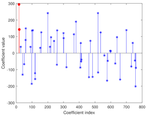
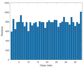
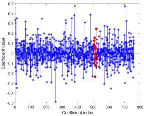
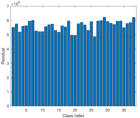
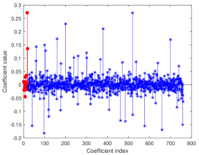
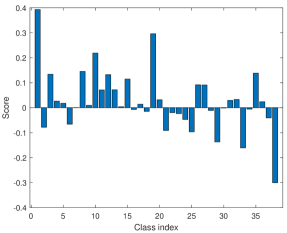
In this section, we present some experimental results on the Extended Yale B database to illustrate the effectiveness of SA-ProCRC. The Extended Yale B database contains 38 individuals and there are about 64 images for each individual. We randomly select 20 images per subject as the training data; therefore, the dictionary contains 760 atoms. We select a test image which belongs to the first subject, and the sparse coefficients and corresponding residual for each class are plotted in Figs. 1 and 2. It can be seen from Fig. 1 that coefficients belong to the first class are prominent. From Fig. 2, we can clearly see that the first class has the least residual, which indicates that the test sample is correctly classified by SRC. Fig. 3 shows the coefficients derived by ProCRC, we can see that the coefficients are rather dense. Fig. 4 presents the residual of ProCRC, one can see that the 26th class has the least residual, thus the test sample is wrongly classified to the 26th class. Coefficients obtained by SA-ProCRC are shown in Fig. 5, we can see that coefficients from the first class are dominant. Fig. 6 plots the score of SA-ProCRC for each class, it can be seen that the first class delivers the largest value. As a result, the test sample is designated to the first class by SA-ProCRC. From the above experimental results, we can find that the dense representation of ProCRC may lead to misclassification. By augmenting the dense representation with a sparse representation, the misclassification can be alleviated. This validates the superiority of our proposed SA-ProCRC.
5 Experiments
In this section, we conduct experiments on four benchmark datasets: the Yale database, the Extended Yale B database, the AR database and the Scene 15 dataset, the details of these datasets are listed in Table 1. We compare the proposed method with state-of-the-art representation based classification methods and several dictionary learning approaches, such as SRC Wright (2009), CRC Zhang (2011), ProCRC Cai (2016), D-KSVD Zhang (2010), LC-KSVD Jiang (2011), FDDL Yang (2011), COPAR Kong (2012), JBDC Akhtar (2017) and SA-CRC Akhtar (2017). For SRC, we solve the problem in Eq. (1) as in Ref. Wright (2009). For CRC, LC-KSVD, FDDL, COPAR, JBDC and SA-CRC, we use the publicly available codes. We adapted the code of LC-KSVD to implement D-KSVD. For SA-CRC and our proposed SA-ProCRC, OMP is utilized to obtain the sparse representation. We utilize the same value of sparsity level (=50) as in SA-CRC Akhtar (2017). All experiments are run with MATLAB R2019a under Windows 10 on PC equipped with 3.60 GHz CPU and 16 GB RAM.
| Dataset | # Sample | # Class | # Feature |
|---|---|---|---|
| Yale | 165 | 15 | 576 |
| EYaleB | 2414 | 38 | 504 |
| AR | 2600 | 100 | 540 |
| Scene 15 | 4485 | 15 | 3000 |
5.1 Experiments on the Yale database
There are 165 images for 15 subjects in the Yale database, each has 11 images. These images have illumination and expression variations, Fig. 7 shows some example images from this database. All the images are resized to 2424 pixels, leading to a 576-dimensional vector. In our experiments, six images per subject are randomly selected for training and the rest for testing. The error tolerance of SRC is 0.05, and the balancing parameter of CRC is 0.001. The sparsity level and number of atoms for D-KSVD and LC-KSVD are 30 and 60, respectively. Sparsity level and of SA-CRC are set to be 50 and 0.002, respectively. Experimental results are summarized in Table 2, in which the best result is highlighted by bold number. It can be observed that SA-ProCRC achieves the highest recognition accuracy, with a 17% reduction in the error rate of ProCRC, and 12% reduction in that of SA-CRC.

| Methods | Accuracy (%) |
|---|---|
| SRC | 95.063.32 |
| CRC | 94.532.97 |
| ProCRC | 95.332.82 |
| D-KSVD | 94.262.88 |
| LC-KSVD | 94.530.03 |
| FDDL | 95.733.00 |
| COPAR | 91.334.23 |
| JBDC | 94.932.72 |
| SA-CRC | 95.602.59 |
| SA-ProCRC | 96.132.84 |
5.2 Experiments on the Extended Yale B database
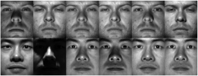
The Extended Yale B face database is composed of 2414 images of 38 individuals. Each individual has 59-64 images taken under different illumination conditions, example images from this dataset are shown in Fig. 8. In our experiments, each 192168 image is projected onto a 504-dimensional space via random projection. 20 images per person are selected for training and the remaining for testing. We use the error tolerance of 0.05 for SRC, and the regularization parameter =0.001 for CRC. The sparsity level and number of atoms for D-KSVD and LC-KSVD are 50 and 400, respectively. Sparsity level and of SA-CRC are set to be 50 and 0.005, respectively. Table 3 lists the recognition accuracy of the comparison methods. It can be seen that our proposed SA-ProCRC is superior to its competing approaches.
| Methods | Accuracy (%) |
|---|---|
| SRC | 93.180.55 |
| CRC | 94.770.48 |
| ProCRC | 94.820.49 |
| D-KSVD | 90.790.51 |
| LC-KSVD | 91.480.69 |
| FDDL | 92.320.68 |
| COPAR | 90.810.55 |
| JBDC | 94.740.83 |
| SA-CRC | 95.520.73 |
| SA-ProCRC | 95.640.78 |
5.3 Experiments on the AR database
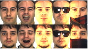
The AR database has more than 4000 face images of 126 subjects with variations in facial expression, illumination conditions and occlusions, Fig. 9 shows example images from this database. We use a subset of 2600 images of 50 male and 50 female subjects from the database. Each 165120 face image is projected onto a 540-dimensional vector by random projection. 10 images per person are randomly selected for training and the remaining for testing. The error tolerance of SRC is 0.05, and the balancing parameter of CRC is 0.0014. The sparsity level and number of atoms for D-KSVD and LC-KSVD are 50 and 600, respectively. Sparsity level and of SA-CRC are set to be 50 and 0.002, respectively. Experimental results are shown in Table 4. We can see that the best classification result is achieved by our proposed SA-ProCRC, with a 23% reduction in the error rate of ProCRC.
| Methods | Accuracy (%) |
|---|---|
| SRC | 91.251.17 |
| CRC | 92.040.83 |
| ProCRC | 93.030.64 |
| D-KSVD | 90.311.13 |
| LC-KSVD | 89.311.27 |
| FDDL | 91.010.99 |
| COPAR | 89.061.54 |
| JBDC | 90.970.79 |
| SA-CRC | 93.740.84 |
| SA-ProCRC | 94.670.66 |
5.4 Experiments on the Scene 15 dataset
This dataset contains 15 natural scene categories including a wide range of indoor and outdoor scenes, such as bedroom, office and mountain, example images from this dataset are shown in Fig. 10. For fair comparison, we employ the 3000-dimensional SIFT-based features used in LC-KSVD Jiang (2011). We randomly select 50 images per category as training data and use the rest for testing. The error tolerance of SRC is 1e-6, and the balancing parameter of CRC is 1. 50 atoms are used for D-KSVD and LC-KSVD. Sparsity level and of SA-CRC are set to be 50 and 1, respectively. Recognition accuracy of different approaches on this dataset are presented in Table 5. Again, SA-ProCRC outperforms the comparison methods.

| Methods | Accuracy (%) |
|---|---|
| SRC | 95.410.13 |
| CRC | 96.150.33 |
| ProCRC | 96.560.35 |
| D-KSVD | 95.120.18 |
| LC-KSVD | 96.370.28 |
| FDDL | 94.080.43 |
| COPAR | 96.020.28 |
| JBDC | 97.360.32 |
| SA-CRC | 97.180.25 |
| SA-ProCRC | 97.560.20 |
6 Conclusions
It has been argued that it is the collaborative representation mechanism rather that the sparsity constraint that makes SRC powerful for pattern classification. As a result, sparsity is ignored to some extent in CRC and its extensions. To address this problem, we present a sparsity augmented probabilistic collaborative representation based classification (SA-ProCRC) method to promote the sparsity in ProCRC. The proposed SA-ProCRC is computationally efficient due to the fact that ProCRC has closed-form solution. Meanwhile, discriminative information contains in the resulting sparse coefficient can be exploited in SA-ProCRC. In essence, SA-ProCRC is a classifier, thus it can be applied to other pattern classification tasks. In our future work, we will evaluate SA-ProCRC with deep features and develop new representation based classification algorithm.
The authors would like to thank Prof. Naveed Akhtar for providing the source code of SA-CRC at http://staffhome.ecm.uwa.edu.au/~00053650/code.html.
The author(s) declared no potential conflicts of interest with respect to the research, authorship, and/or publication of this article.
The author(s) disclosed receipt of the following financial support for the research, authorship, and/or publication of this article: This work was supported by the National Natural Science Foundation of China (Grant No. 61672265).
References
- Wright (2009) Wright J, Yang A Y, Ganesh A, et al. Robust face recognition via sparse representation. IEEE TPAMI, 2009, 31: 210-227.
- Wang (2016) Wang Y, Tang Y Y, Li L. Correntropy matching pursuit with application to robust digit and face recognition. IEEE Trans. on Cybernetics, 2016, 47(6): 1354-1366.
- Wu (2018) Wu C Y, Ding J J. Occluded face recognition using low-rank regression with generalized gradient direction. Pattern Recognition, 2018, 80: 256-268.
- Gao (2017) Gao G, Yang J, Jing X Y, et al. Learning robust and discriminative low-rank representations for face recognition with occlusion. Pattern Recognition, 2017, 66: 129-143.
- Keinert (2019) Keinert F, Lazzaro D, Morigi S. A Robust group-sparse representation variational method with applications to face recognition. IEEE Trans. on Image Processing, 2019, 28(6): 2785-2798.
- Qiao (2010) Qiao L, Chen S, Tan X. Sparsity preserving projections with applications to face recognition. Pattern Recognition, 2010, 43(1): 331-341.
- Cui (2018) Cui Y, Jiang J, Lai Z, et al. An integrated optimisation algorithm for feature extraction, dictionary learning and classification. Neurocomputing, 2018, 275: 2740-2751.
- Xie (2018) Xie L, Yin M, Yin X, et al. Low-rank sparse preserving projections for dimensionality reduction. IEEE Trans. on Image Processing, 2018, 27(11): 5261-5274.
- Zhang (2018) Zhang T, Xu C, Yang M H. Robust structural sparse tracking. IEEE PAMI, 2018, 41(2): 473-486.
- Liu (2016) Liu Y, Chen X, Ward R K, et al. Image fusion with convolutional sparse representation. IEEE Signal Processing Letters, 2016, 23(12): 1882-1886.
- Guo (2019) Guo T, Luo F, Zhang L, et al. Target detection in hyperspectral imagery via sparse and dense hybrid representation. IEEE Geoscience and Remote Sensing Letters, 2019.
- Zhang (2015) Zhang Z, Xu Y, Yang J, et al. A survey of sparse representation: algorithms and applications. IEEE Access, 2015, 3: 490-530.
- Akhtar (2017) Akhtar N, Shafait F, Mian A. Efficient classification with sparsity augmented collaborative representation. Pattern Recognition, 2017, 65: 136-145.
- Zhang (2011) Zhang L, Yang M, Feng X. Sparse representation or collaborative representation: Which helps face recognition? In CVPR, Colorado Springs, Colorado, 20-25 June 2011, pp.471-478.
- Cai (2016) Cai S, Zhang L, Zuo W, et al. A probabilistic collaborative representation based approach for pattern classification. In CVPR, Las Vegas, Nevada, 27-30 June 2016, pp.2950-2959.
- Tropp (2007) Tropp J A, Gilbert A C. Signal recovery from random measurements via orthogonal matching pursuit. IEEE Trans. on Information Theory, 2007, 53(12): 4655-4666.
- Zhang (2010) Zhang Q, Li B. Discriminative K-SVD for dictionary learning in face recognition. In CVPR, San Francisco, California, 13-18 June, 2010, pp.2691-2698.
- Jiang (2011) Jiang Z, Lin Z, Davis L S. Learning a discriminative dictionary for sparse coding via label consistent K-SVD. In CVPR, Colorado Springs, Colorado, 20-25 June 2011, pp.697-1704.
- Yang (2011) Yang M, Zhang L, Feng X, et al. Fisher discrimination dictionary learning for sparse representation. In CVPR, Colorado Springs, Colorado, 20-25 June 2011, pp.543-550.
- Kong (2012) Kong S, Wang D. A dictionary learning approach for classification: separating the particularity and the commonality. In ECCV, Florence, Italy, 7-13 October 2012, pp.186-199.
- Akhtar (2017) Akhtar N, Mian A, Porikli F. Joint discriminative Bayesian dictionary and classifier learning. In CVPR, Honolulu, Hawaii, 21-26 July 2017, pp.1193-1202.