A Neural Networks study of the phase transitions of Potts model

Abstract

Using the techniques of Neural Networks (NN), we study the three-dimensional (3D) 5-state ferromagnetic Potts model on the cubic lattice as well as the two-dimensional (2D) 3-state antiferromagnetic Potts model on the square lattice. Unlike the conventional approach, here we follow the idea employed in Ann. Phy. 391 (2018) 312-331. Specifically, instead of numerically generating numerous objects for the training, the whole or part of the theoretical ground state configurations of the studied models are considered as the training sets. Remarkably, our investigation of these two models provides convincing evidence for the effectiveness of the method of preparing training sets used in this study. In particular, the results of the 3D model obtained here imply that the NN approach is as efficient as the traditional method since the signal of a first order phase transition, namely tunneling between two channels, determined by the NN method is as strong as that calculated with the Monte Carlo technique. Furthermore, the outcomes associated with the considered 2D system indicate even little partial information of the ground states can lead to conclusive results regarding the studied phase transition. The achievements reached in our investigation demonstrate that the performance of NN, using certain amount of the theoretical ground state configurations as the training sets, is impressive.

I Introduction

During the last couple years, the application of methods and techniques of artificial intelligence (AI) in many-body systems has drawn tremendous attention in the physics community Rup12 ; Sny12 ; Mer14 ; Sch14 ; Li15 ; Lee16 ; Wan16 ; Oht16 ; Car16 ; Tro16 ; Tor16 ; Bro16 ; Chn16 ; Tan16 ; Nie16 ; Liu16 ; Xu16 ; Wan17 ; Liu17 ; Che17 ; Nag17 ; Den17 ; Pon17 ; Zha17 ; Zha17.1 ; Hu17 ; Li18 ; Chn18 ; Bea18 ; Sha18 ; Zha18 ; Gao18 ; Zha19 ; Gre19 ; Don19 ; Yoo19 ; Can19 ; Lia19 . For example, by employing the idea of restricted Boltzmann machine, it is demonstrated that the efficiency of certain Monte Carlo simulations can be improved dramatically Wan17 . In addition, with the supervised and unsupervised Neural Networks (NN), the critical points and exponents, as well as the nature of the phase transitions of some classical and quantum models are determined with high accuracy Wan16 ; Oht16 ; Car16 ; Tro16 ; Tor16 ; Bro16 ; Chn16 ; Nie16 ; Hu17 ; Li18 . These applications of AI in physics are very successful. Hence it is anticipated that the ideas of AI not only provide alternative approaches for studying many-body systems, but also have great potential in exploring properties of materials that are beyond what have been achieved using the traditional methods.

The standard (conventional) procedure of applying supervised NN to investigate the phase transitions of physics systems consists of three steps, namely the training, the validation, and the testing stages. Taking two-dimensional (2D) Ising model on the square lattice as an example Car16 , in the testing stage, typical configurations at various temperatures below and above the transition temperature $T_{c}$ are generated by Monte Carlo simulations or other numerical techniques. Moreover, labels of $(1,0)$ and $(0,1)$ are assigned to all the generated configurations below and above $T_{c}$, respectively. Through the optimization procedure, the desired weights are determined and are used in later computations in both the validation and testing stages. The role of the validation stage is to make sure that correct outcomes are obtained using the trained NN (weights). Finally, in the testing stage, output results at many temperatures acrossing $T_{c}$ are determined. In particular, the temperature at which the output is $(0.5,0.5)$ is expected to be the $T_{c}$.

Using the procedures described in the previous paragraph, it is demonstrated that the $T_{c}$ of 2D Ising model on the square lattice indeed can be calculated accurately using a supervised NN Car16 . Furthermore, NN can even detect incorrect information and precisely determine $T_{c}$ Nie16 . Such a conventional approach also applies to other models and success to certain satisfactory extent are obtained.

While it seems promising that in the near future, methods of AI may play an important role in studying many-body systems, when it comes to examine the critical phenomena, what are the benefits of using the NN techniques rather than employing the traditional methods needs further investigation. In particular, it is crucial to explore which of the traditional and the NN approaches performs better. Besides, the conventional strategy for the training stage introduced above has a caveat, namely $T_{c}$ is known in prior before making a use of NN. As a result, for a new system without the knowledge of its critical point, it may be difficult to employ the conventional approach to train the NN in a straightforward manner.

To overcome this issue mentioned above regarding studying a phase transition with a unknown critical point, instead of generating configurations numerically for the training, in Ref. Li18 the expected ground state configurations are used as the training sets of a NN investigation for the phase transitions of 2D $Q$-state ferromagnetic Potts models on the square lattice Wu82 . Using this strategy, $T_{c}$ is not essential in using the NN method and there is very little computation effort required for generating the training sets. With such an unconventional approach, success of calculating the associated $T_{c}$ and determining the nature of the phase transitions of 2D $Q$-state ferromagnetic Potts models are reached Li18 .

Although one can locate $T_{c}$ and determine the nature of phase transitions accurately for $Q$-state ferromagnetic Potts models with the idea of using the theoretical ground state configurations as the training sets, it should be pointed out that for a given positive integer $Q$, there are $Q$ ground state configurations for $Q$-state ferromagnetic Potts model and all these configurations can be used as the training set like that being done in Ref. Li18 , without encountering any technical difficulty. An interesting question arise regarding the applicability of the this approach. Specially, if only part of all the ground state configurations are employed as the training set, will the resulting NN still be able to reach the success as that shown in Ref. Li18 ? This is an important effect to examine when systems with highly degenerated ground states are studied using the NN techniques.

In addition to studying critical phenomena, the application of AI methods in the majority fields of science requires the use of real data points as the training sets. Indeed, such a combination advances certain areas of research greatly. Still, it will be extremely compelling to understand whether solely AI techniques can achieve the same level of success as that obtained by the traditional methods.

Motivated by these subtle issues described above, here we consider NN which are trained without using any actual data as the training sets. Furthermore, we employ the built NN to study the three-dimensional (3D) 5-state ferromagnetic Potts model on the cubic lattice as well as the 2D 3-state antiferromagnetic Potts model on the square lattice. The reasons that these two models are chosen will be explained later.

Interestingly, our study for the 3D model indicates that NN is as efficient as the traditional Monte Carlo method since the signal of a first order phase transition, namely tunneling between two channels, determined by the NN method is as strong as that calculated with the Monte Carlo technique. This result suggests that NN is a promising alternative approach for studying many-body systems. Furthermore, the NN outcomes obtained for the considered 2D system provide convincing evidence that using the ideas considered in Ref. Li18 , even little partial information of the ground states can lead to conclusive results regarding the studied phase transition. To summarize, the performance of NN, using certain amount of the theoretical ground state configurations as the training set, is impressive.

This paper is organized as follows. After the introduction, the studied microscopic models and the details of the employed NN are described. In particular, the NN training sets and labels are introduced thoroughly. Following this the resulting numerical results by applying the Monte Carlo simulations and the NN techniques are presented. Finally, a section concludes our investigation.

II The microscopic models and observables

The Hamiltonian $H$ of $Q$-state Potts model considered in our study is given by Wu82 ; Swe87 ; Wan89 ; Wan90

$$\beta H=-J\beta\sum_{\left<ij\right>}\delta_{\sigma_{i},\sigma_{j}},$$ (1)

where $\beta$ is the inverse temperature and $\left<ij\right>$ stands for the nearest neighboring sites $i$ and $j$. In addition, in Eq. (1) the $\delta$ refers to the Kronecker function and finally, the Potts variable $\sigma_{i}$ appearing above at each site $i$ takes an integer value from $\{1,2,3,...,Q\}$. The situations of $J>0$ and $J<0$ correspond to ferromagnetic and antiferromagnetic Potts models, respectively.

As already being mentioned previously, in this study we focus on investigating the phase transitions of 3D 5-state ferromagnetic Potts model on the cubic lattice and 2D 3-state antiferromagnetic Potts model on the square lattice. The motivations for considering these two models are as follows.

First of all, it is known that the phase transition of 3D 5-state ferromagnetic Potts model on the cubic lattice is first order Wu82 . Furthermore, the signal of a first order phase transition becomes exponentially hard to observe as the space-time volume increases Bil95 ; Non15 . Therefore, studying 3D 5-state ferromagnetic Potts model on the cubic lattice provides an opportunity to compare the efficiency of detecting a first order phase transition between the traditional and NN approaches.

The 2D 3-state antiferromagnetic Potts model on the square lattice is studied here because it is shown that its associated phase transition occurs at zero temperature Wan90 ; Kun95 ; Fer99 . In other words, the system is disordered at any $T>0$. As a result, the conventional training strategy usually employed in a NN investigation of a many-body system may not be applicable for this model. Hence the 2D 3-state antiferromagnetic Potts model on the square lattice serves as a good testing ground for the NN approach of using the theoretical ground state configurations as the training set.

The obserbables considered here for the 3D 5-state ferromagnetic Potts model are the energy density $E$ and the magnetization density $\langle|m|\rangle$. Here $m$ is defined as

$$m=\frac{1}{L^{3}}\sum_{j}\exp\left(i\frac{2\pi\sigma_{j}}{5}\right),$$ (2)

where $L$ is the linear box sizes used in the calculations and the summation is over all lattice sites $j$. Moreover, to study the 2D 3-state antiferromagnetic Potts model on the square lattice, the staggered magnetization density $m_{s}$, which takes the form

$$m_{s}=\frac{1}{3}\sum_{i=1}^{3}|M_{i}|,$$ (3)

is measured in our simulations. Here $M_{i}$ is defined as

$$M_{i}=\frac{2}{L^{2}}\sum_{x}(-1)^{x_{1}+x_{2}}\delta_{\sigma_{x},i},$$ (4)

where again the summation is over all lattice sites $x$. Finally, Potts configurations for both the considered models are recorded as well and will be used in the calculations related to NN.

III The constructed supervised Neural Networks

In this section, we will introduce the details of the supervised NN used in our study. The employed training sets and the associated labels will be described as well. Moreover, we will consider the simplest NN of deep learning and examine whether it can reach the same level of success as those obtained with complicated NN such as the convolutional Neural Networks (CNN).

III.1 The built multilayer perceptron (MLP)

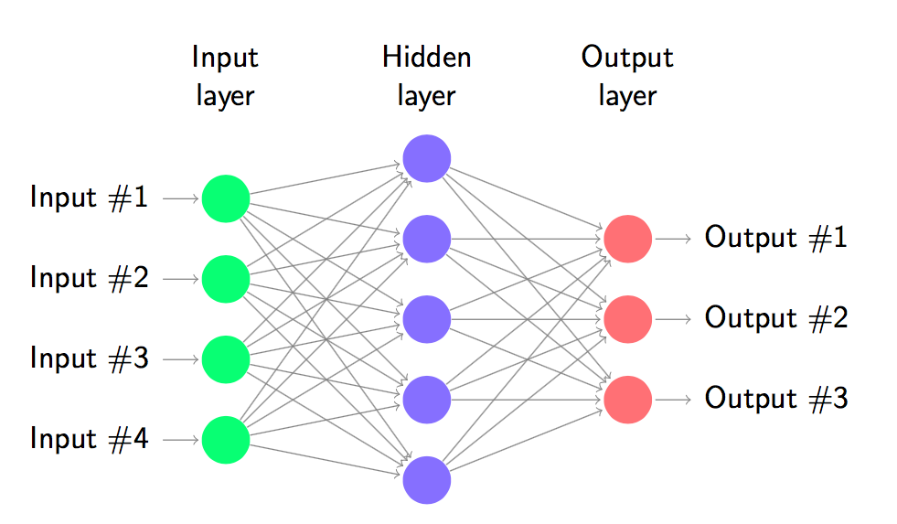
Since we would like to understand whether the simplest deep learning NN (multilayer perceptron, MLP) is capable of detecting the critical point, the supervised NN considered in our investigation consists of only one input layer, one hidden layer of 512 independent nodes, and one output layer using the publicly available NN libraries keras and tensorflow kera ; tens . Fig. 1 demonstrates the NN used here. The algorithm, optimizer, and loss function we employ for the calculations are minibatch, adam, and categorical cross entropy, respectively. $L_{2}$ regularization is applied as well to avoid overfitting. The activation functions considered are ReLU (between the input layer and hidden layer) and softmax (between the hidden layer and output layer). In addition, for the 3D model, computations using various batchsize, nodes, copies of the pre-training set (defined later), and epoch are conducted as well. Moreover, the weights obtained in the training processes which minimize the loss function are recorded and are used in later calculations. Finally, to understand the impact on the output results from the initial values of weights as well as other steps performed in the training stage, several sets of random seeds are used in the investigation. For the studied 2D antiferromagnetic model, all the outcomes obtained with various random seeds will be considered in determining the final results associated with this model.

Figure 1: The NN (MLP) used in this study.

III.2 Training set and output labels for the 3D model

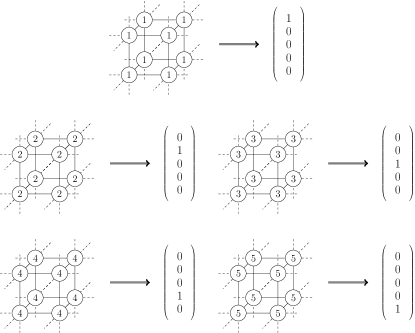
Regarding the training set used for the 3D 5-state ferromagnetic Potts model on the cubic lattice, we will follow the idea considered in Ref. Li18 , namely the employed training set consists of 200 (or any suitable number) copies of the corresponding theoretical ground state configurations. The expected ground state configurations for 3D 5-state ferromagnetic Potts model on a $L\times L\times L$ cubic lattice are obtained by letting the Potts variables on all the lattice sites take the same (positive) integer from $\{1,2,3,4,5\}$ as their values. Consequently, there are 5 ground state configurations. The associated labels for these 5 ground state configurations are the basis vectors of five-dimensional (5D) Euclidean space. While not being unique, clearly one can construct an one to one correspondence between the 5 ground state configurations and the basis vectors of 5D Euclidean space. One of such correspondence is shown in fig. 2. These five ground state configurations will be named pre-training set in this study. Finally, we would like to emphasize the fact that when constructing the pre-training set, all the allowed Potts variables should be used.

Figure 2: Pre-training set and their corresponding labels considered here for the 3D 5-state ferromagnetic Potts model on the cubic lattice.

III.3 The expected output vectors for the 3D model at various $T$

With such a set up of pre-training set, it is expected that at extremely low temperatures, the norm ($R$) of the NN output vectors are around 1 since most of the Potts variables take the same positive integer $Q_{1}$ as their values. As a result, one component of the associated output vector has much larger magnitude than that of the others. The norm of such a vector clearly is around 1.

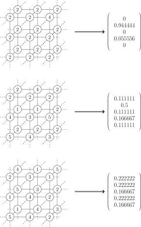
As the temperature arises, some Potts variables begin to obtain other positive integers than $Q_{1}$. Consequently, the magnitude of norm of the output vectors diminishes with $T$. When $T\geq T_{c}$, the norm of NN output vectors are around its minimum value $1/\sqrt{5}$. This is because there is an equal probability that each integer in $\{1,2,3,4,5\}$ is the value of any Potts variables. The cartoon plots shown in fig. 3 demonstrates how the Potts configurations and the corresponding output vectors change with $T$. Based on this scenario of $R$ versus $T$, $T_{c}$ can be estimated to lie within the temperature window at which $R$ decreases rapidly from 1 to $1/\sqrt{5}$. Indeed such a method is shown to be able to determine $T_{c}$ with high precision in Ref. Li18 . For a more detailed introduction to this approach of using the theoretical ground state configurations as the training set, including its validation, we refer the readers to Ref. Li18 .

Figure 3: The expected Potts configurations and the corresponding NN output vectors at low temperatures ($T\ll T_{c}$, top panel), moderate temperature ($T<T_{c}$, middle panel), and high temperature ($T\geq T_{c}$, bottom panel) for the studied 3D model. The output vectors are for demonstration, not the real ones.

III.4 Training set and output labels for the 2D model

Similar to the strategy introduced in the previous subsection, here we will employ the expected ground state configurations as the pre-training set for the NN study associated with the considered 2D system. Unlike the ferromagnetic Potts model, any two nearest neighboring Potts variables for the ground state configurations of 2D $Q$-state antiferromagnetic Potts model differ from each other. As a result, there are tremendous number of such configurations when $Q\geq 3$. We construct 6, 18, and 36 expected ground state configurations of the 2D 3-state antiferromagnetic Potts model and use these configurations as the pre-training sets. The unit blocks (2 by 2 lattices and their Potts variables) for the built 6 configurations are shown in fig. 4, and configurations on larger lattices are obtained by multiplying any of these 6 unit blocks by itself several times in both the $x$- and $y$-direction (The associated labels which will be introduced shortly are demonstrated in fig. 3 as well). Using these pre-training sets, the actual training sets are a multiple copy (Here we use a factor of 200) of the pre-training sets.

The output labels used here for the pre-training sets follows exactly the ones in the previous subsection related to the 3D 5-state ferromagnetic Potts model. For instance, for the pre-training set consisting of 6 configurations, the corresponding labels are the basis vectors of 6-dimensional Euclidean space. Clearly, similar to the case of ferromagnetic Potts model, one can map these 6 configurations in the pre-training set onto the 6 basis vectors of 6-dimensional Euclidean space in an one to one manner (This map is not unique as well). The same construction rule applies when 18 or 36 configurations are considered as the pre-training set, see fig. 5 for part of the pre-training sets consisting of 18 and 36 configurations.

Remarkably, although in this study only very little information of the whole ground state configurations are employed as the training sets, as we will demonstrate shortly, the built NN with the designed training sets and labels is capable of showing convincing evidence that the phase transition of the investigated 2D 3-state antiferromagnetic Potts model occurs only at zero temperature as the theory predicts.

Figure 4: Unit blocks (2 by 2 lattices and their Potts variables) for building the pre-training set consisiting of 6 configurations, and their corresponding labels considered here for the 2D 3-state antiferromagnetic Potts model on the square lattice.

                         

Figure 5: Several unit blocks for building pre-training sets consisiting of 18 (left, 2 by 2 lattices and their Potts variables) and 36 (right, 4 by 4 lattices and their Potts variables) configurations, for the 2D 3-state antiferromagnetic Potts model on the square lattice. Configurations on larger lattices are obtained by multiplying any of these unit blocks by itself several times in both the $x$- and $y$-direction.

IV Numerical results

To generate configurations of the studied 2D and 3D Potts models, which will be used in the testing stages of the NN procedures, Swendsen and Wang algorithm Swe87 , Wolff algorithm Wol89 , as well as Swendsen-Wang-Kotecky algorithm Wan89 ; Wan90 are adopted. Particularly, Potts configurations are stored once in every thousand (or two thousand) Monte Carlo sweeps after the thermalization.

Figure 6: Energy density $E$ (top panel) as a function of MC sweep and the histogram of magnetization density $\langle|m|\rangle$ (bottom panel) near $T_{c}$ of the 3-state ferromagnetic Potts model on the cubic lattice. The associated box size $L$ and $\beta$ for the data shown in this figure are $L=16$ and $\beta=0.689$, respectively

IV.1 Results of 3D 5-state ferromagnetic Potts model

IV.1.1 The Monte Carlo results

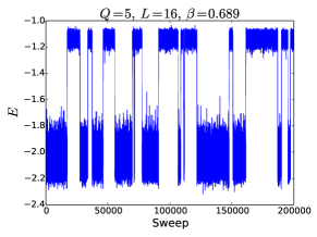
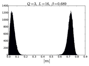
In fig. 6, the energy density $E$ as a function of MC sweep (top panel), and the histogram of the magnetization density $\langle|m|\rangle$ (bottom panel) at a temperature close to $T_{c}$ for the 3D 5-state ferromagnetic Potts model on the cubic lattice are shown. The outcomes are obtained with $L=16$ and $\beta=0.689$. The phenomenon of tunneling between two values clearly appear in the top panel of the figure. In addition, two peaks structure shows up as well in the bottom panel of fig. 6. These are the features of a first order phase transition. In other words, our Monte Carlo data confirm the theoretical prediction that the phase transition of 3D 5-state ferromagnetic Potts model on the cubic lattice is discontinuous.

IV.1.2 The NN results

Figure 7: $R$ as functions of $T$ for the 3D 5-state ferromagnetic Potts model on the cubic lattice with $L=12$. The vertical dashed line is the expected $T_{c}$. Results obtained using different parameter sets are all shown in the figure.

Figure 8: $R$ as functions of $T$ for the 3D 5-state ferromagnetic Potts model on the cubic lattice with $L=12,16$. The vertical dashed line is the expected $T_{c}$.

Figure 9: The histogram of $R$ at a temperature near the $T_{c}$ of 3D 5-state ferromagnetic Potts model on the cubic lattice. The associated box size $L$ and $\beta$ for the data shown in this figure are $L=16$ and $\beta=0.689$, respectively

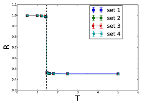
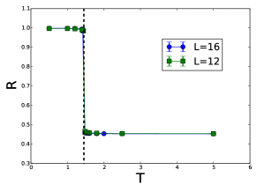
The norm $R$ of the output vectors as functions of $T$ for the 3D 5-state Potts model on the cubic lattice are demonstrated in fig. 7. The vertical dashed line which appears in the figure is the expected $T_{c}$. These results are obtained on $12$ by $12$ by $12$ lattices. Moreover, for a fixed $T$ four calculations using different parameters of random seeds, batchsize, copies of the pre-training set, and epoch are conducted and all the obtained resulting $R$ are shown in fig. 7. The outcomes in fig. 7 indicate that $R$ is very stable with respect to the tunable variables associated with NN. In addition, as can be seen from the figure as well as that of fig. 8 which includes the outcomes of $L=16$, the magnitude of $R$ decreases rapidly in the temperature region close to the theoretical $T_{c}$. Based on this result and that of Ref. Li18 , it is beyond doubt that for $Q$-state ferromagnetic Potts model, the associated $T_{c}$ can be precisely estimated to lie within the temperature window at which the magnitude of $R$ drops sharply from 1 to 1/$\sqrt{Q}$

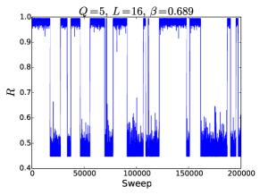
Fig. 9 shows the histogram of $R$ for the 3D 5-state ferromagnetic Potts model on the cubic lattice at a temperature $T$ near $T_{c}$. The outcome is obtained with $L=16$ and $\beta=0.689$. A clear two peaks structure obviously appears in the figure. As a result, the studied phase transition is first order. In other words, the NN constructed here, which consists of only one input layer, one hidden layer, and one output layer, is capable of not only locating $T_{c}$ precisely, but also determining the nature of the phase transition of the investigated model. It is anticipated that the built NN can carry out similar calculations with success for general $Q$-state ferromagnetic Potts models in any dimension and on any lattice geometry.

IV.2 Results of 2D 3-state antiferromagnetic Potts model

IV.2.1 The Monte Carlo results

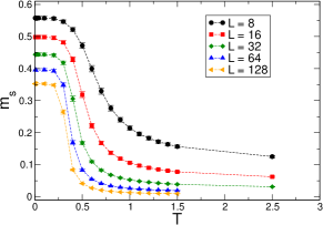
In fig. 10 the staggered magnetization density $m_{s}$ as functions of temperature $T$ for the considered 2D 3-state ferromagnetic Potts model on the square lattice are presented. In particular, outcomes corresponding to various $L$ are shown in the figure. The results in the figure demonstrate that for every finite $L$, the magnitude of its corresponding magnetization diminishes as $T$ rises and eventually at high temperature $m_{s}$ reaches a saturated value which is anticipated to go to zero when $L\rightarrow\infty$. Moreover, for the simulated box sizes, the curves shown in the figure do not intersect among themselves. Such a scenario is interpreted as the phase transition takes place at zero temperature, namely the system is always in the disordered phase at any $T>0$.

Figure 10: $m_{s}$ as functions of $T$ for the 2D 3-state antiferromagnetic Potts model on the square lattice. Results associated with various box sizes $L$ are shown in the figure.

IV.2.2 The NN results

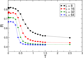
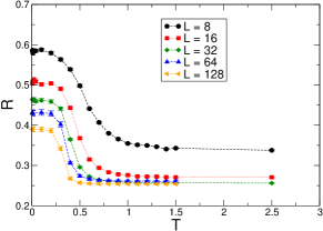
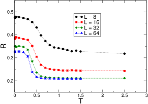
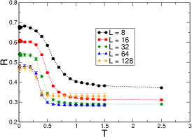
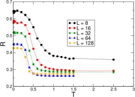
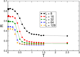
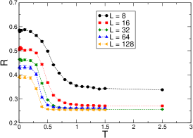
The NN outcomes of $R$ as functions of $T$ for various training sets (using 6, 18, and 36 constructed configurations as the pre-training sets) are shown in figs. 11, 12, 13, and the shown data are obtained using ten results. In particular, each of these results is calculated with its own set of random seeds which is different from that of the others. These figures, which are obtained using different training sets, all demonstrate similar characteristics as that of $m_{s}$ (fig. 10). Specifically, the $T$-$R$ curves of various $L$ have the trend that the magnitude of $R$ decrease monotonically with $T$. In addition, for every employed training set, the associate $T$-$R$ curves do not intersect among themselves except those of larger $L$, which can be interpreted as the size convergence of the NN outcomes.

We would like to point out that for the results of using 18 configurations as the pre-training set (i.e fig. 12), in the high temperature region $R$ of $L=64$ are slightly above that of $L=32$ (not within statistical errors). We attribute this to the systematic uncertainty due to the tunable parameters of NN that are not taken into account here. Nevertheless, considering the similarity between the results of NN and MC (i.e. figs. 10, 11, 12, 13), the outcomes of NN provide convincing numerical evidence that the phase transition of 2D 3-state antiferromagnetic Potts model on the square lattice occurs at zero temperature.

When compared with that of the studied 3D model, the NN outcomes of the 2D 3-state antiferromagnetic Potts model have (much) larger uncertainties. Indeed, for the calculations using various random seeds, while the variation among the resulting $R$ associated with the considered 3D model is negligible, the uncertainty of R related to the studied 2D model has sizable magnitude. Similarly, other tunable parameters in the used NN such as the batchsize have certain impact on the outcomes of $R$ of the antiferromagnetic system. We further find that in order to obtain results consistent with that determined from Monte Carlo simulations, the ratio $p$ between how many objects in the training set and the considered batchsize has to be a number with moderate magnitude. Since $p$ is associated with the independent parameters during the optimization procedure, too many or too few free parameters will lead to not satisfactory outcomes from the optimization considering the limitation of the algorithm employed in this process.

Using 18 configurations as the pre-training set, the NN outcomes of $R$ for various $T$ and $L$ obtained using batchsizes 40, 80, 160, and 320 are shown in fig. 14 (from top to bottom). As can be seen in that figure, when batchsize is 40 the corresponding data of $L=128$ lie well above those of $L=32,64$ in the high temperature region. This is in contradiction with the Monte Carlo results. As the batchsize increases, the trend of $R$ versus $T$ for various box sizes $L$ become more and more similar to that of MC. Finally, the outcomes shown in the bottom panel of fig. 14 which is calculated with batchsize 320 are consistent, at least qualitatively, with that of MC. Our investigation of 2D 3-state antiferromagnetic Potts model on the square lattice indicate that cautions have to be taken, when NN techniques are considered to study physics systems having highly degenerated ground state configurations.

Finally, we would like to emphasize the fact that the results shown in each of figs. 11, 12, 13 are obtained using the same variables of NN for all the considered box sizes $L=8,16,32,64(128)$. It is likely that the most suitable parameters associated with NN for various $L$ could be different. In other words, for complicated systems, carrying out certain fine tuning to search appropriate parameters of NN may be required in order to reach the right signals of physics.

Figure 11: $R$ as function of $T$ for various box sizes $L$. These results are obtained using 6 configurations as the pre-training set and the considered batch size is 40.

Figure 12: $R$ as functions of $T$ for various box sizes $L$. These results are obtained using 18 configurations as the pre-training set and the considered batch size is 320.

Figure 13: $R$ as functions of $T$ for various box sizes $L$. These results are obtained using 36 configurations as the pre-training set and the considered batch size is 320.

V Discussions and Conclusions

Figure 14: $R$ as functions of $T$ for various box sizes $L$. These results are obtained using 18 configurations as the pre-training set and the employed batch sizes are 40, 80, 160, and 320 (from top to bottom).

In this study we investigate the phase transitions of 3D 5-state ferromagnetic Potts model and 2D 3-state antiferromagnetic Potts model, using both the Monte Carlo calculations and techniques of NN. The NN considered here has the simplest deep learning structure, namely it consists of one input layer, one hidden layer, and one output layer. Moreover, unlike the conventional approach of using data generated by numerical methods for the training, in our study we employ full or part of the theoretical ground state configurations as the (pre-)training sets.

The conventional training of a NN typically requires the use of actual data points. In particular, the knowledge of the critical point ($T_{c}$) is essential to study the associated phase transition using the standard approach of NN methods. Our strategy for the training process has the advantage that information of $T_{c}$ is not necessary to carry out the investigation and very little computation effort is needed for generating the training sets. The magnitude of the output vectors $R$ is shown to be the relevant quantity to locate the critical points as well as to determine the nature of the phase transitions.

Remarkably, the NN results related to the studied 3D models obtained here imply that even a simplest NN of deep learning can lead to highly accurate determination of $T_{c}$. Furthermore, the quantity $R$ used here is as efficient as that typically considered in the traditional methods when it comes to decide the nature of the considered phase transitions. Interestingly, the tunneling phenomena in figs. 6 and 9 indicate that, whenever $E$ reaches the results of large numerical values, $R$ obtains the outcomes with small magnitude and vice-versa. In other words, $R$ and $E$ are complementary to each other and $R$ indeed reflects the correct physics.

For the 2D 3-state antiferromagnetic Potts model, we have carried out the NN investigation using 6, 18, and 36 theoretical ground state configurations of this model as the (pre-)training sets. While the resulting NN outcomes with certain constraints on the tunable parameters are consistent with the Monte Carlo results, it is subtle to reach the correct physics from the NN calculations. Indeed, as we have demonstrated here, the variation among NN results obtained with different random seeds and batchsize are not negligible. In particular, the ratio of the number of training objects and the batchsize plays a crucial role in obtaining outcomes having the right signals of physics. In summary, one has to pay special attention when models having highly degenerated ground state configurations are investigated using the NN method. For such cases, certain fine tuning to search appropriate parameters of NN may be required in order to observe the correct physics.

To conclude, here we reconfirm the validity of the training approach considered in Ref. Li18 . In particular, we succeed in applying this method to the study of the phase transition of 2D 3-state antiferromagnetic Potts model on the square lattice, which takes place at zero temperature and may be difficult to detect using the conventional NN training procedure. It remains interesting to examine whether the method employed in this study is capable of precisely calculating other relevant physical quantities at phase transitions, such as the critical exponents.

References

- (1) Matthias Rupp, Alexandre Tkatchenko, Klaus-Robert Müller, and O. Anatole von Lilienfeld, Phys. Rev. Letts. 108 058301 (2012).
- (2) John C. Snyder, Matthias Rupp, Katja Hansen, Klaus-Robert Müller, and Kieron Burke, Phys. Rev. Letts. 108 253002 (2012).
- (3) B. Meredig, A. Agrawal, S. Kirklin, J. E. Saal, J. W. Doak, A. Thompson, K. Zhang, A. Choudhary, and C. Wolverton, Phys. Rev. B 89, 094104 (2014).
- (4) K. T. Schütt, H. Glawe, F. Brockherde, A. Sanna, K. R. Müller, and E. K. U. Gross, Phys. Rev. B 89, 205118 (2014).
- (5) Zhenwei Li, James R. Kermode, and Alessandro De Vita, Phys. Rev. Lett. 114, 096405 (2015)
- (6) Joohwi Lee, Atsuto Seko, Kazuki Shitara, Keita Nakayama, and Isao Tanaka, Phys. Rev. B 93, 115104 (2016).
- (7) Lei Wang, Phys. Rev. B 94, 195105 (2016)
- (8) Tomoki Ohtsuki and Tomi Ohtsuki, J. Phys. Soc. Jpn. 85, 123706 (2016).
- (9) Juan Carrasquilla, Roger G. Melko, Nature Physics 13, 431–434 (2017).
- (10) Giuseppe Carleo, Matthias Troyer, Science 355, 602 (2017)
- (11) Giacomo Torlai and Roger G. Melko, Phys. Rev. B 94, 165134 (2016).
- (12) Peter Broecker, Juan Carrasquilla, Roger G. Melko, and Simon Trebst, Scientific Reports 7, 8823 (2017).
- (13) Kelvin Ch’ng, Juan Carrasquilla, Roger G. Melko, and Ehsan Khatami, Phys. Rev. X 7, 031038 (2017).
- (14) Akinori Tanaka, Akio Tomiya, J. Phys. Soc. Jpn. 86, 063001 (2017).
- (15) Evert P.L. van Nieuwenburg, Ye-Hua Liu, Sebastian D. Huber, Nature Physics 13, 435–439 (2017)
- (16) Junwei Liu, Huitao Shen, Yang Qi, Zi Yang Meng, Liang Fu, Phys. Rev. B 95, 241104(R) (2017).
- (17) Xiao Yan Xu, Yang Qi, Junwei Liu, Liang Fu, Zi Yang Meng, Phys. Rev. B 96, 041119(R) (2017).
- (18) Li Huang and Lei Wang, Phys. Rev. B 95, 035105 (2017).
- (19) Junwei Liu, Yang Qi, Zi Yang Meng, Liang Fu, Phys. Rev. B 95, 041101 (2017).
- (20) Qianshi Wei, Roger G. Melko, Jeff Z. Y. Chen, Phys. Rev. E 95, 032504 (2017).
- (21) Yuki Nagai, Huitao Shen, Yang Qi, Junwei Liu, and Liang Fu Phys. Rev. B 96 161102 (2017).
- (22) Dong-Ling Deng, Xiaopeng Li, and S. Das Sarma, Phys. Rev. B 96 195145 (2017).
- (23) Pedro Ponte and Roger G. Melko, Phys. Rev. B 96, 205146 (2017).
- (24) Yi Zhang, Roger G. Melko, and Eun-Ah Kim Phys. Rev. B 96, 245119 (2017).
- (25) Yi Zhang and Eun-Ah Kim, Phys. Rev. Lett. 118, 216401 (2017)
- (26) Wenjian Hu, Rajiv R. P. Singh, and Richard T. Scalettar, Phys. Rev. E 95, 062122 (2017).
- (27) C.-D. Li, D.-R. Tan, and F.-J. Jiang, Annals of Physics, 391 (2018) 312-331.
- (28) Kelvin Ch’ng, Nick Vazquez, and Ehsan Khatami, Phys. Rev. E 97, 013306 (2018).
- (29) Matthew J. S. Beach, Anna Golubeva, and Roger G. Melko, Phys. Rev. B 97, 045207 (2018).
- (30) Phiala E. Shanahan, Daniel Trewartha, and William Detmold, Phys. Rev. D 97, 094506 (2018).
- (31) Pengfei Zhang, Huitao Shen, and Hui Zhai, Phys. Rev. Letts. 120, 066401 (2018).
- (32) Jun Gao et al. Phys. Rev. Letts. 120, 240501 (2018).
- (33) Wabzhou Zhang, Jiayu Liu, Jiayu and Tzu-Chieh Wei, Phys. Rev. E 99, 032142 (2019).
- (34) Jonas Greitemann, Ke Liu, and Lode Pollet, Phys. Rev. B 99, 060404 (2019).
- (35) Xiao-Yu Dong, Frank Pollmann, and Xue-Feng Zhang, Phys. Rev. B 99, 121104 (2019).
- (36) Boram Yoon, Tanmoy Bhattacharya, and Rajan Gupta, Rajan Phys. Rev. D 100, 014504 (2019).
- (37) Askery Canabarro, Felipe Fernandes Fanchini, André Luiz Malvezzi, Rodrigo Pereira, and Rafael Chaves, Phys. Rev. B 100, 045129 (2019).
- (38) Wenqian Lian et al., Phys. Rev. Letts. 122, 210503 (2019).
- (39) F. Y. Wu, Rev. Mod. Phys. 54, 235 (1982).
- (40) R. H. Swendsen, and J.-S. Wang, (1987), Phys. Rev. Lett. 58(2), 86 (1987).
- (41) J.-S. Wang, R. H. Swendsen, and R. Kotecky, Phys. Rev. Lett. 63, 109 (1989).
- (42) Jian-Sheng Wang, Robert H. Swendsen, and Roman Kotecky, Phys. Rev. B 42, 2465 (1990).
- (43) Alain Billoire, arXiv:hep-lat/9501003.
- (44) Yoshihiko Nonomura and Yusuke Tomita, Phys. Rev. E 92, 062121 (2015).
- (45) U. Wolff, Phys. Rev. Lett. 62, 361 (1989).
- (46) P. J. Kundrotas, S. Lapinskas, and A. Rosengren Phys. Rev. B 52, 9166 (1995).
- (47) Ferreira, S.J. and Sokal, A.D., Journal of Statistical Physics (1999) 96: 461.
- (48) https://keras.io
- (49) https://www.tensorflow.org