Triangle singularity appearing as an $X(3872)$-like peak in $B\to(J/\psi\pi^{+}\pi^{-})K\pi$

Abstract

We consider a triangle diagram for $B^{0}\to(J/\psi\pi^{+}\pi^{-})K^{+}\pi^{-}$ where an $X(3872)$ peak has been observed experimentally. We demonstrate that a triangle singularity inherent in the triangle diagram creates a sharp peak in the $J/\psi\pi^{+}\pi^{-}$ invariant mass distribution when the final $(J/\psi\pi^{+}\pi^{-})\pi$ invariant mass is at and around the $D^{*}\bar{D}^{*}$ threshold. The position and width of the peak is 3871.68 MeV (a few keV above the $D^{*0}\bar{D}^{0}$ threshold) and $\sim$0.4 MeV, respectively, in perfect agreement with the precisely measured $X(3872)$ mass and width: $3871.69\pm 0.17$ MeV and $<1.2$ MeV. This remarkable agreement is virtually parameter-free. The result indicates that the considered mechanism has to be understood in advance when separating an $X(3872)$-pole contribution from $B^{0}\to(J/\psi\pi^{+}\pi^{-})K^{+}\pi^{-}$ data; the separation yields an $X(3872)\pi$ lineshape that could be used to determine the $X(3872)$ mass. We suggest a method to set a constraint on the triangle mechanism by analyzing a charge analogous process $B^{0}\to(J/\psi\pi^{0}\pi^{-})K^{+}\pi^{0}$ where a similar triangle singularity generates an $X^{-}(3876)$-like peak.

I Introduction

Establishing the existence of exotic hadrons, which are not accommodated by the conventional quark model picture qm , is arguably the most prioritized problem in the contemporary hadron spectroscopy. The discovery of $X(3872)$ belle_x3872_jpsi-rho triggered this trend where the nature of $X(3872)$ has always been the central problem; see Refs. review_swanson ; review_voloshin ; review_chen ; review_hosaka ; review_lebed ; review_esposito ; review_ali ; review_guo ; review_olsen ; review_raphael for reviews. Experimentally, $X(3872)$ has been observed not only in $B$ meson decays where it was discovered belle_x3872_jpsi-rho ; babar_x3872_jpsi-rho , but also in $pp$ and $\bar{p}p$ collisions cdf_x3872_jpsi-rho ; d0_x3872_jpsi-rho ; lhcb_x3872_jpsi-rho and $e^{+}e^{-}$ annihilations bes3_x3872_jpsi-rho . $X(3872)$ has been confirmed to decay into several channels such as $J/\psi\rho^{0}(\rho^{0}\to\pi^{+}\pi^{-})$ belle_x3872_jpsi-rho ; babar_x3872_jpsi-rho ; cdf_x3872_jpsi-rho ; d0_x3872_jpsi-rho ; lhcb_x3872_jpsi-rho ; bes3_x3872_jpsi-rho , $J/\psi\omega$ babar_x3872_jpsi-omega ; bes3_x3872_jpsi-omega , $J/\psi\gamma$ belle_x3872_jpsi-gamma , $D^{*0}\bar{D}^{0}$ belle_x3872_ddstar , and more.

Figure 1: Triangle diagrams (A,B) [(C,D)] contributing to $B^{0}\to J/\psi\rho^{0}K^{+}\pi^{-}$ [$B^{0}\to J/\psi\rho^{-}K^{+}\pi^{0}$]. The diagrams (A,C,D) cause triangle singularities to generate a sharp peak in $J/\psi\rho$ invariant mass ($M_{J/\psi\rho}$) distributions at $M_{J/\psi\rho}\sim 3.872,3.876$ and 3.875 GeV, respectively. From the left to right, we refer to the diagrams in the text as diagrams A, B, C, and D, respectively.

Many theoretical attempts have been made to understand what $X(3872)$ consists of. Because of the close proximity of its mass to the $D^{*0}\bar{D}^{0}$  threshold, a $D^{*0}\bar{D}^{0}$ molecule is a popular idea swanson_molecule ; zhao_molecule . However, a pure molecule picture makes it difficult to understand its formation rate in the hadron collider experiments suzuki . Thus a superposition of the molecule with an excited charmonium is considered more plausible suzuki ; Kalashnikova ; takizawa . The latest Lattice QCD lqcd_Prelovsek ; lqcd_Padmanath found a state that could be identified with $X(3872)$, and disfavored diquark-antidiquark interpretations tetra_maiani ; tetra_chen . Yet, it seems difficult to reach a consensus on the structure of $X(3872)$ within the so-far proposed ideas (maybe except for Lattice QCD) because of lots of unknowns concerning the relevant hadron dynamics, and one may fine-tune them to reproduce available data.

Another issue is that a spectrum peak of $X(3872)$ could be partly faked by a kinematical effect, the triangle singularity (TS) in particular. A TS occurs from a triangle diagram like Fig. 1 only if a special kinematical condition is realized: all three internal particles are simultaneously on-shell and their momenta are collinear like in a classical process landau ; coleman ; s-matrix . The TS can significantly enhance the amplitude, and can show up as a bump in, for example, $J/\psi\rho$ and $J/\psi\rho\pi$ invariant mass distributions of the processes in Fig. 1. For mathematical details and practical use, we refer the readers to Ref. TS-Pc2 . Attempts have been made to interpret some $XYZ$ exotic candidates as bumps due to TSs ts1_z3900 ; ts2_z3900 ; szczepaniak ; xhliu1 ; xhliu2 ; xhliu3 ; ts4_z3900 ; ts3_z3900 ; ts_zc4430 ; ts_z4050 ; ts_review .

The triangle diagram of Fig. 1(A)  for $B^{0}\to J/\psi\rho^{0}K^{+}\pi^{-}$ satisfies conditions to create an $X(3872)$-like peak in the $J/\psi\rho^{0}$ invariant mass distribution when the $J/\psi\rho^{0}\pi^{-}$ invariant mass is at and around the $D^{*-}D^{*0}$ threshold. Experimentally, an $X(3872)$ peak has been observed in the $J/\psi\pi^{+}\pi^{-}$ lineshape of $B^{0}\to(J/\psi\pi^{+}\pi^{-})K^{+}\pi^{-}$ belle_x3872kpi ; belle_x3872kpi2  . In this work, we demonstrate that the TS inherent in the triangle diagram generates an exactly $X(3872)$-like peak in the $J/\psi\pi^{+}\pi^{-}$ invariant mass spectrum. The spectrum peak position and shape agrees with the $X(3872)$ mass measured at $\sim$0.01% precision and the tightly constrained width without any fine-tuning of the model parameters.

Our analysis will indicate that the TS should be taken into account when studying $X(3872)$ in $B^{0}\to J/\psi\rho^{0}K^{+}\pi^{-}$ in the TS region. This would be particularly relevant to an idea recently proposed by Guo guo_x3872 ; sakai_x3872 ; sakai2_x3872 on determining the $X(3872)$ mass from $X(3872)\pi$ and $X(3872)\gamma$ lineshapes. Characteristic lineshapes are created by TSs of triangle diagrams similar to the diagram A but different in including an $X(3872)$-pole propagation as $D^{*0}\bar{D}^{0}\to X(3872)\to J/\psi\rho^{0}$ . The idea is based on the fact that the lineshapes sensitively change depending on the $X(3872)$ mass. Because $X(3872)\to J/\psi\pi^{+}\pi^{-}$ is suppressed by an isospin violation, the isospin conserving non-resonant process like the diagram A could give a comparable $X(3872)$-like contribution as a background for the $X(3872)$ mass analysis. In order to understand the non-resonant mechanism and separate it from the $X(3872)$-pole contribution, we will suggest to analyze a charge analogous $B^{0}\to(J/\psi\pi^{0}\pi^{-})K^{+}\pi^{0}$ decay for which TSs from related triangle diagrams C and D generates an $X^{-}(3876)$-like peak.

II model

The $B^{0}\to J/\psi\rho^{0}K^{+}\pi^{-}$ amplitude from the triangle diagram A can be written, in the $J/\psi\rho^{0}\pi^{-}$ center-of-mass (CM) frame, as

$$T = \int d\bm{q}\,v_{J/\psi\rho^{0};D^{*0}\bar{D}^{0}}\,{1\over W-E_{D^{*0}}-E_{\bar{D}^{0}}-E_{\pi^{-}}}$$

$$\times\Gamma_{\bar{D}^{0}\pi^{-},D^{*-}}{1\over W-E_{D^{*-}}-E_{D^{*0}}}V_{K^{+}D^{*-}D^{*0},B^{0}}\,,$$

where $\bm{q}$ is a loop momentum. The invariant mass of the $J/\psi\rho^{0}\pi^{-}$ subsystem is denoted by $W$, while the energy of a particle $x$ is $E_{x}$ which depends on the particle mass ($m_{x}$) and momentum ($\bm{p}_{x}$) as $E_{x}=\sqrt{\bm{p}^{2}_{x}+m^{2}_{x}}-i\Gamma_{x}/2$; $\Gamma_{x}$ is the decay width which is nonzero for $D^{*}$. The summation of intermediate spin states is implied. We use values from the Particle Data Group (PDG) pdg for the particle masses ($m_{x}$), except for the final $\rho$ meson for which our treatment will be discussed later. Amplitudes for triangle diagrams B, C, and D are similar. In calculating observables for the $B^{0}\to J/\psi\rho^{0}K^{+}\pi^{-}$ ($B^{0}\to J/\psi\rho^{-}K^{+}\pi^{0}$) decay, the triangle mechanisms A and B (C and D) must be coherently added. Because of the charge-parity invariance and isospin symmetry of the strong interaction, the triangle mechanisms A and B (C and D) exactly cancel with each other in a hypothetical situation where the charged and neutral $D^{*}$ mesons have the same mass and width. In reality, the cancellation is incomplete; the TS peaks are mostly intact while contributions away from the TS region are largely cancelled.

We emphasize that mass differences between the isospin partners such as $({\pi^{\pm}},{\pi^{0}})$, $({D^{+}},{D^{0}})$, and $({D^{*+}},{D^{*0}})$, must be taken into account because they are essentially important whether or not a TS exists in the triangle diagrams. Indeed, while the triangle diagrams A, C, and D cause TSs, the diagram B does not. This is because $D^{*0}\to D^{+}\pi^{-}$ at on-shell is kinematically forbidden and thus the kinematical condition for TS is not satisfied. The triangle amplitude of Eq. (LABEL:eq:amp) for the diagram A in the zero-width limit causes a TS in the kinematical range of:

$$0 < M_{J/\psi\rho}-(m_{D^{*0}}+m_{D^{0}})\leq 0.2~{}{\rm MeV}\ ,$$ (2)

$$0 < W-(m_{D^{*-}}+m_{D^{*0}})\ \raise 1.29167pt\hbox{$<$\kern-7.5pt\lower 4.30554pt\hbox{$\sim$}}\ 1.0~{}{\rm MeV}\ ,$$ (3)

where $M_{J/\psi\rho}$ denotes the $J/\psi\rho$ invariant mass. Although finite widths would relax the singularity, the $D^{*-}$ and $D^{*0}$ widths are very small as discussed in the next paragraph. Therefore we expect from the TS a very sharp peak at $M_{J/\psi\pi^{+}\pi^{-}}\sim m_{D^{*0}}+m_{D^{0}}=3871.7$ MeV that coincides with the $X(3872)$ mass. Similarly, the TS condition is satisfied for the triangle diagram C in

$$0 < M_{J/\psi\rho}-(m_{D^{*0}}+m_{D^{-}})\leq 0.2~{}{\rm MeV}\ ,$$ (4)

with $m_{D^{*0}}+m_{D^{-}}=3876.4$ MeV, and for the diagram D

$$0 < M_{J/\psi\rho}-(m_{D^{*-}}+m_{D^{0}})\leq 0.2~{}{\rm MeV}\ ,$$ (5)

with $m_{D^{*-}}+m_{D^{0}}=3875.1$ MeV; the $W$ range is the same as Eq. (3). Thus the coherent sum of the diagrams C and D is expected to give a sharp $X^{-}(3876)$-like peak in the $M_{J/\psi\pi^{0}\pi^{-}}$ distribution.

Regarding the $D^{*\pm}$ decay width, we use the central value of the PDG average, $\Gamma_{D^{*\pm}}=83.4\pm 1.8$ keV pdg . On the other hand, the $D^{*0}$ decay width has been given an upper limit only, $\Gamma_{D^{*0}}<2.1$ MeV pdg . Thus we use $\Gamma_{D^{*0}}$ calculated by assuming the isospin symmetry between $D^{*+}\to D^{+}\pi^{0}$ and $D^{*0}\to D^{0}\pi^{0}$, and also by taking account of the experimentally determined branching to $D^{*0}\to D^{0}\gamma$ pdg . We obtain $\Gamma_{D^{*0}}=55$ keV which is very similar to those derived previously guo_x3872 ; rosner_dstar . We use the constant $D^{*}$ width values in Eq. (LABEL:eq:amp), which has been checked to be a very good approximation.

An $s$-wave $D^{*0}\bar{D}^{0}\to J/\psi\rho^{0}$ interaction we use in Eq. (LABEL:eq:amp) is

$$v_{J/\psi\rho^{0};D^{*0}\bar{D}^{0}}\,=f^{01}_{J/\psi\rho^{0}}(p)f^{01}_{D^{*0}\bar{D}^{0}}(p^{\prime})\,\bm{\epsilon}^{*}_{J/\psi}\times\bm{\epsilon}^{*}_{\rho}\cdot\bm{\epsilon}_{D^{*0}}\ ,$$ (6)

where $\bm{\epsilon}_{x}$ denotes the polarization vector for a vector meson $x$. The $J/\psi\rho^{0}$ pair coming out of this interaction has the spin-parity $J^{P}=1^{+}$ because of the spin combination specified by the interaction. Thus, if the $J/\psi\rho^{0}$ pair generates a bump in the invariant mass ($M_{J/\psi\rho}$) distribution, the pair seems like a decay product of a resonance of $J^{P}=1^{+}$, the spin-parity of $X(3872)$. We have used in Eq. (6) dipole form factors $f^{LS}_{ij}(p)$ defined by

$$f^{LS}_{ij}(p)=g^{LS}_{ij}{p^{L}\over\sqrt{E_{i}(p)E_{j}(p)}}\left(\frac{\Lambda^{2}}{\Lambda^{2}+p^{2}}\right)^{2+(L/2)}\ ,$$ (7)

where $L$ ($S$) is the orbital angular momentum (total spin) of the $ij$ pair; $p=|\bm{p}_{ij}|$ with $\bm{p}_{ij}$ the $i$’s momentum in the $ij$ CM frame. We use a cutoff $\Lambda=1$ GeV in the form factors throughout unless otherwise stated. The coupling strength ($g^{LS}_{ij}$) for the interaction of Eq. (6) is little known and thus left arbitrary. Microscopically, this contact interaction can be viewed as an axial vector $D_{1}$-meson exchange or a quark exchange mechanism swanson_molecule . An $X(3872)$-pole contribution is not included in $v_{J/\psi\rho^{0};D^{*0}\bar{D}^{0}}$.

The vertex function for $D^{*-}\to\bar{D}^{0}\pi^{-}$ is denoted by $\Gamma_{\bar{D}^{0}\pi^{-},D^{*-}}$ in Eq. (LABEL:eq:amp), and its explicit form is given in a general form as

$$\Gamma_{ij,R}(\bm{p}_{i},\bm{p}_{j};\bm{p}_{R}) = \sum_{LS}f^{LS}_{ij}(p_{ij})(s_{i}s_{i}^{z}s_{j}s_{j}^{z}|SS^{z})$$ (8)

$$\times (LMSS^{z}|S_{R}S^{z}_{R})Y_{LM}(\hat{p}_{ij})\ ,$$

where $Y_{LM}$ is spherical harmonics. We use a notation of $(abcd|ef)$ as Clebsch-Gordan coefficients in which we write the spin of a particle $x$ $s_{x}$ and its $z$-component $s_{x}^{z}$. The coupling strength $g^{10}_{\bar{D}^{0}\pi^{-}}$ included in the form factor $f^{10}_{\bar{D}^{0}\pi^{-}}$ is determined by fitting the partial decay width for $D^{*-}\to\bar{D}^{0}\pi^{-}$ pdg .

The $B^{0}\to D^{*-}D^{*0}K^{+}$ decay vertex in Eq. (LABEL:eq:amp) is expressed with two vertex functions of Eq. (8) as

$$V_{K^{+}D^{*-}D^{*0},B^{0}} = \exp\left(-b\ {W-m_{D^{*-}}-m_{D^{*0}}\over m_{D^{*-}}+m_{D^{*0}}}\right)$$ (9)

$$\times\sum_{\cal R}\Gamma_{D^{*-}D^{*0},{\cal R}}(\bm{p}_{D^{*-}},\bm{p}_{D^{*0}};\bm{p}_{\cal R})$$

$$\times\Gamma_{K^{+}{\cal R},B^{0}}(\bm{p}_{K^{+}},\bm{p}_{{\cal R}};\bm{p}_{B^{0}})\ ,$$

where “states” ${\cal R}$ have been introduced just for conveniently representing $J^{P}$ of the $D^{*-}D^{*0}$ pair; ${\cal R}$ is not a propagating state. We consider $J^{P}=0^{+}$ and $s$-wave for the $D^{*-}D^{*0}$ pair; the other $J^{P}$ does not change the main conclusion which is essentially determined by the TS.

We introduced the exponential factor in Eq. (9) where the parameter $b$ characterizes the $W$-dependence of the vertex. Although there is no experimental information to fix the $W$-dependence, possibly related information is available from other processes such as the $M_{D^{*}\bar{D}^{*}}$ distributions from $e^{+}e^{-}\to J/\psi D^{*}\bar{D}^{*}$ belle-pakhlov and $e^{+}e^{-}\to(D^{*}\bar{D}^{*})^{\pm}\pi^{\mp}$ bes3_z4020 ; both data show significant enhancements near the $D^{*}\bar{D}^{*}$ threshold. We assume that the $M_{D^{*}\bar{D}^{*}}$ distribution of $B^{0}\to D^{*-}D^{*0}K^{+}$ is similar to these data, and that the $D^{*-}D^{*0}$ $s$-wave decay vertex of Eq. (9) dominates in the whole $W$ region. Then we can fix the parameter $b$ in Eq. (9) as $b=30$ for the cutoff $\Lambda=1$ GeV. The resulting $M_{D^{*}\bar{D}^{*}}$ distribution is shown in Fig. 2. After fixing the $W$ dependence, we can determine the $B^{0}\to D^{*-}D^{*0}K^{+}$ vertex strength using data for the branching ratio: ${\cal B}(B^{0}\to D^{*-}D^{*0}K^{+})=1.06\pm 0.03\,({\rm stat.})\pm 0.086\,({\rm syst.})$% babar_BDDK . Since the triangle diagrams in Fig. 1 hit TSs only at $W\sim m_{D^{*-}}+m_{D^{*0}}$, the $W$-dependence is unimportant for thsee proceeses in the TS region. We note that the $X(3872)$ mass determination method guo_x3872 ; sakai_x3872 ; sakai2_x3872 analyzes the $W$-dependence only near and in the TS region. However, the $M_{J/\psi\pi^{+}\pi^{-}}$ lineshape for $B^{0}\to(J/\psi\pi^{+}\pi^{-})K^{+}\pi^{-}$ from the Belle belle_x3872kpi includes data from the whole $W$ region. Because the $W$-integrated $M_{J/\psi\pi^{+}\pi^{-}}$ lineshape depends on the $W$-dependence, we manage it as above in order to compare the model with the data.

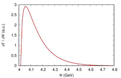
Figure 2: $W$-dependence of the $B^{0}\to D^{*-}D^{*0}K^{+}$ differential decay width from the decay vertex of Eq. (9). No rescattering is considered.

We evaluate the interactions of Eqs. (6) and (8) in the CM frame of the two-body subsystem, and then multiply kinematical factors to account for the Lorentz transformation to the $J/\psi\rho^{0}\pi^{-}$ CM frame; see Appendix C of Ref. 3pi for details.

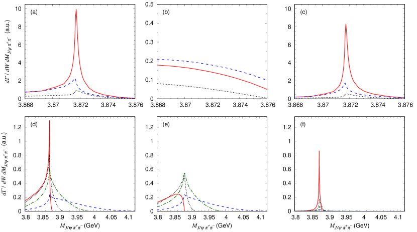
Figure 3: $J/\psi\pi^{+}\pi^{-}$ invariant mass ($M_{J/\psi\pi^{+}\pi^{-}}$) distributions from the triangle diagrams of Figs. 1(A) and 1(B) for $B^{0}\to J/\psi\pi^{+}\pi^{-}K^{+}\pi^{-}$. $J/\psi$ is paired with $\pi^{+}\pi^{-}$ from $\rho^{0}$ decay to give $M_{J/\psi\pi^{+}\pi^{-}}$. (Upper) The TS region. The black dotted, red solid, and blue dashed curves correspond to the spectra at $W-(m_{D^{*0}}+m_{D^{*-}})=-1.0$, 0.0, and 1.2 MeV, respectively, where $W$ is the invariant mass of the final $J/\psi\pi^{+}\pi^{-}\pi^{-}$ subsystem and $m_{D^{*0}}+m_{D^{*-}}=4017.1$ MeV. (Lower) Higher $W$ region. The red solid, black dotted, green dash-dotted, and blue dashed curves correspond to the spectra at $W-(m_{D^{*0}}+m_{D^{*-}})=2.7$, 32.8, 112.8, and 258.3 MeV, respectively. In the upper [lower] panels, the triangle diagrams of Figs. 1(A) and 1(B) generate the spectra in the panels (a) and (b) [(d) and (e)], respectively, and their coherent sum is given in the panel (c) [(f)]. While the vertical scale is arbitrary, the relative scales among the curves in all the panels are the model-prediction and not arbitrary.

The double differential decay width, $d\Gamma_{B\to J/\psi\rho^{0}K\pi}/dWdM_{J/\psi\rho}$, is calculated with the decay amplitude of Eq. (LABEL:eq:amp) in a standard manner as detailed in Appendix B of Ref. 3pi . We then take account of the $\rho^{0}\to\pi^{+}\pi^{-}$ decay. Thus the final expression for the double differential decay width is given by

$${d\Gamma_{B\to J/\psi\pi^{+}\pi^{-}K\pi}\over dWdM_{J/\psi\pi^{+}\pi^{-}}} = \int{dM_{\pi\pi}\over 2\pi}\left.{d\Gamma_{B\to J/\psi\rho^{0}K\pi}\over dWdM_{J/\psi\rho^{0}}}\right|_{m_{\rho^{0}}=M_{\pi\pi}}$$

$$\times{[M_{\pi\pi}/E_{\rho^{0}}]^{2}\,\Gamma_{\rho^{0}\to\pi^{+}\pi^{-}}(M_{\pi\pi})\over|\tilde{W}-E_{\rho^{0}}+{i\over 2}\Gamma_{\rho^{0}}(M_{\pi\pi})|^{2}}\,,$$

where $\tilde{W}\equiv W-E_{J/\psi}-E_{\pi}$ and the $\rho^{0}$ nominal mass ($\bar{m}_{\rho^{0}}=775$ MeV) is used only in $E_{\rho^{0}}=\sqrt{\bar{m}^{2}_{\rho^{0}}+\bm{p}^{2}_{\rho^{0}}}$. The total and partial $\rho^{0}$ decay widths are denoted by $\Gamma_{\rho^{0}}$ and $\Gamma_{\rho^{0}\to\pi^{+}\pi^{-}}$, respectively, and the $M_{\pi\pi}$ dependence is given by $\Gamma_{\rho^{0}}/\bar{\Gamma}_{\rho^{0}}=(q/\bar{q})(\bar{m}_{\rho^{0}}/M_{\pi\pi})^{2}[f^{10}_{\pi\pi}(q)/f^{10}_{\pi\pi}(\bar{q})]^{2}$ where $q$ is the pion momentum in the $\rho^{0}$ rest frame; the quantities with bar corresponds to the case of $M_{\pi\pi}=\bar{m}_{\rho^{0}}$ and $\bar{\Gamma}_{\rho^{0}}=150$ MeV; the form factor $f^{10}_{\pi\pi}(q)$ has been defined in Eq. (7).

III results

III.1 $X(3872)$-like TS peak in $B^{0}\to(J/\psi\pi^{+}\pi^{-})K^{+}\pi^{-}$

We show in Figs. 3(a,d), 3(b,e), and 3(c,f) the $M_{J/\psi\pi^{+}\pi^{-}}$ distributions of the double differential decay width $d\Gamma_{B^{0}\to J/\psi\pi^{+}\pi^{-}K^{+}\pi^{-}}/dWdM_{J/\psi\pi^{+}\pi^{-}}$, defined in Eq. (LABEL:eq:decay), from the triangle diagrams A, B, and A+B, respectively. The spectra in and near the TS region ($W\sim m_{D^{*0}}+m_{D^{*-}}$) are shown in Fig. 3(a-c) where the prominent feature is a very sharp peak created by the TS from the diagram A at $M_{J/\psi\pi^{+}\pi^{-}}\sim 3871.7$ MeV, exactly falling on the precisely measured $X(3872)$ mass: $3871.69\pm 0.17$ MeV pdg . We stress that the peak position and the narrow width due to the TS is virtually parameter-free. The cutoff dependence over $\Lambda=0.5-2$ GeV has been confirmed not to significantly change the position and shape of the TS peak, and the other arbitrary parameters can change only the overall normalization. This stability stems from the facts that: (i) the TS dominates because the tiny $D^{*}$ width puts the TS very close to the physical region; (ii) the TS does not depend on dynamical details. We also find the acute sensitivity of the TS peak to $W$, reflecting the fact that the TS region is within a small window of $W$ as in Eq. (3).

Meanwhile, the triangle diagram B gives smooth lineshapes for $W\sim m_{D^{*0}}+m_{D^{*-}}$ as seen in Fig. 3(b). This sharp contrast between the diagrams A and B is from the fact that the TS condition is satisfied by the diagram A only. Although one might have expected a smaller enhancement arising from the diagram B because of its proximity to the TS condition, this is not the case. The high selectivity of the TS condition shown here is in part due to the smallness of the $D^{*}$ width. The role played by the diagram B in the coherent sum shown in Fig. 3(c) is to remove the smooth background-like contribution from the diagram A.

The $M_{J/\psi\pi^{+}\pi^{-}}$ distributions for higher $W$ region are given in Fig. 3(d-f). Figure 3(d) shows that the remnant of the TS peak from the diagram A quickly disappears as $W$ increases, and the threshold cusp stays at $M_{J/\psi\pi^{+}\pi^{-}}=m_{D^{*0}}+m_{\bar{D}^{0}}$ in the higher $W$ region. The cusp height for higher $W$ is shorter due to the $W$ dependence of the $B^{0}\to D^{*-}D^{*0}K^{+}$ decay vertex introduced in Eq. (9). The diagram B also generates similar cusps at slightly higher energy of $M_{J/\psi\pi^{+}\pi^{-}}=m_{D^{*-}}+m_{D^{+}}$ as seen in Fig. 3(e). Thus the coherent sum leaves just a small differece between contributions from the diagrams A and B as shown in Fig. 3(f).

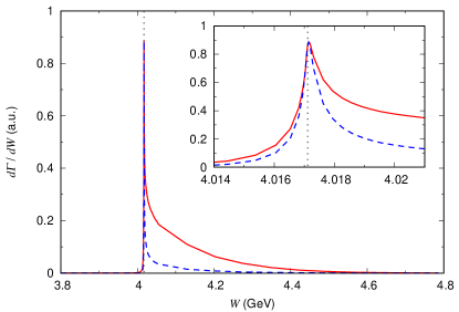
Figure 4: $W$ dependence of $B^{0}\to J/\psi\pi^{+}\pi^{-}K^{+}\pi^{-}$ decay rate from the coherent sum of the triangle diagrams of Figs. 1(A) and 1(B). The red solid curve is obtained by integrating the spectrum in Fig. 3(c,f) with respect to $M_{J/\psi\pi^{+}\pi^{-}}$ at each $W$. The blue dashed curve is obtained similarly but the integral is limited to the range of $3.871\leq M_{J/\psi\pi^{+}\pi^{-}}\leq 3.8725$ GeV. For a better visibility, the blue dashed curve has been scaled by a factor of 1.95. The vertical line indicates the $D^{*-}D^{*0}$ threshold. The insert shows the peak region.

Integrating the spectra in Fig. 3(c,f) over $M_{J/\psi\pi^{+}\pi^{-}}$ at each $W$ gives $d\Gamma_{B^{0}\to J/\psi\pi^{+}\pi^{-}K^{+}\pi^{-}}/dW$ which is shown in Fig. 4 by the red solid curve. The spectrum sharply rises and peaks slightly above the $D^{*-}D^{*0}$ threshold, and then falls off. Because the $W$ dependence of the spectra in Fig. 3(c) is particularly strong around the peak, we expect an even stronger $W$ dependence of $d\Gamma_{B^{0}\to J/\psi\pi^{+}\pi^{-}K^{+}\pi^{-}}/dW$ if we limit the integral with respect $M_{J/\psi\pi^{+}\pi^{-}}$ to a range around $M_{J/\psi\pi^{+}\pi^{-}}\sim 3871.7$ MeV. This is indeed the case as shown by the blue dashed curve in Fig. 4.

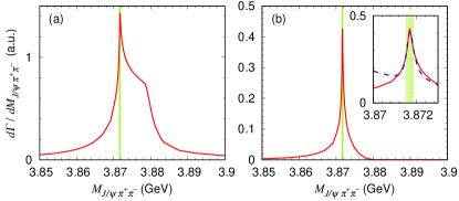
Figure 5: $M_{J/\psi\pi^{+}\pi^{-}}$ distributions from the triangle diagrams of Figs. 1(A) and 1(B). (a) The red solid curve is obtained from the spectra in Fig. 3(c,f) by integrating with respect to $W$ over the whole $W$-region as shown in Fig. 4. (b) The red solid curve is obtained similarly, but the integral is limited to the range of $-3~{}{\rm MeV}\leq W-(m_{D^{*-}}+m_{D^{*0}})\leq 4~{}{\rm MeV}$. The insert shows the peak region. The blue dashed curve is the Breit-Wigner plus a background fitted to the red solid curve. The green bands indicate the $X(3872)$ mass range from the PDG pdg .

The Belle data on $d\Gamma_{B^{0}\to J/\psi\pi^{+}\pi^{-}K^{+}\pi^{-}}/dM_{J/\psi\pi^{+}\pi^{-}}$ for $B^{0}\to J/\psi\pi^{+}\pi^{-}K^{+}\pi^{-}$ belle_x3872kpi ; belle_x3872kpi2 , showing the peak at $M_{J/\psi\pi^{+}\pi^{-}}\sim 3.872$ GeV, is from the whole kinematically allowed $W$ region. To obtain a theoretical counterpart, we integrate the spectra in Fig. 3(c,f) with respect to $W$. The resulting spectrum is shown in Fig. 5(a). We find a sharp peak at $M_{J/\psi\pi^{+}\pi^{-}}\sim 3.872$ GeV, and also a large shoulder near the $D^{*-}D^{+}$ threshold. We smeared the spectrum by the experimental resolution, and found that the lineshape is too broad to be compatible with the data. This shape depends on the $W$-dependence of the $B^{0}\to D^{*-}D^{*0}K^{+}$ vertex specified in Eq. (9). As the higher $W$ region is more suppressed, the shoulder shrinks more. Although our choice of the $W$-dependence can be different from the reality to some extent, it seems unlikely that the diagrams A and B can explain the Belle data.

Table 1: Breit-Wigner mass ($m_{BW}$) and width ($\Gamma_{BW}$). The parameters in the second column are determined by fitting the $M_{J/\psi\pi^{+}\pi^{-}}$ spectrum of Fig. 5(b) from the triangle diagrams of Figs. 1(A) and 1(B). The parameter ranges are from the cutoff dependence ($\Lambda=0.5-2$ GeV). The PDG values for $X(3872)$ are shown in the third column.

	Figs. 1(A)+1(B)	$X(3872)$ (PDG pdg )
$m_{BW}$ (MeV)	$3871.68\pm 0.00$	$3871.69\pm 0.17$
$\Gamma_{BW}$ (MeV)	$0.42\pm 0.01$	$<1.2$

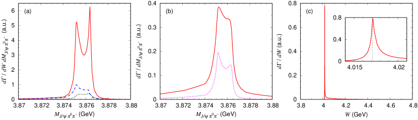
Figure 6: $M_{J/\psi\pi^{0}\pi^{-}}$ and $W$ distributions for $B^{0}\to J/\psi\pi^{0}\pi^{-}K^{+}\pi^{0}$ from the coherently summed triangle diagrams of Figs. 1(C) and 1(D). $J/\psi$ is paired with $\pi^{0}\pi^{-}$ from $\rho^{-}$ decay to give $M_{J/\psi\pi^{0}\pi^{-}}$. (a) The black dotted, red solid, and blue dashed curves correspond to $M_{J/\psi\pi^{0}\pi^{-}}$ distributions at $W-(m_{D^{*0}}+m_{D^{*-}})=-1.0$, 0.0, and 1.2 MeV, respectively. (b) The red solid curve is obtained from the spectra in the panel (a) by integrating over $W$. The magenta dotted curve is obtained similarly, but the integral range is limited to $-3~{}{\rm MeV}\leq W-(m_{D^{*-}}+m_{D^{*0}})\leq 4~{}{\rm MeV}$. (c) The red solid curve is obtained by integrating the spectra in the panel (a) with respect to $M_{J/\psi\pi^{0}\pi^{-}}$ at each $W$. The vertical line indicates the $D^{*-}D^{*0}$ threshold. The TS peak region is enlarged in the insert. Regarding the vertical scale, the curves in the panels (a), (b), and (c) are comparable to those in Figs. 3, 5, and 4, respectively.

We now limit the $W$-integral to near and in the TS region, $-3~{}{\rm MeV}\leq W-(m_{D^{*-}}+m_{D^{*0}})\leq 4~{}{\rm MeV}$, and show the obtained spectrum by the red solid curve in Fig. 5(b). This time, the narrow peak clearly remains. To see the peak position and width quantitatively, we simulate the spectrum with the conventional resonance($X$)-excitation mechanism, $B\to XK\pi$ followed by $X\to J/\psi\rho^{0}$, and determine the Breit-Wigner mass and width of $X$. We also add a coherent background contribution given by an adjustable quadratic polynomial of $M_{J/\psi\pi^{+}\pi^{-}}$. The result of the fit is shown by the blue dashed curve in the insert of Fig. 5(b). The quality of the fit in the tail region is not very good because: (i) the peak shape is rather different from the Breit-Wigner form; (ii) the background is a quickly decreasing function of $M_{J/\psi\pi^{+}\pi^{-}}$ near the higher end at $\sim 3.88$ GeV due to the limited phase-space. Still, the obtained Breit-Wigner parameters would be useful to characterize the peak, and are presented in Table 1 and compared with the PDG value for $X(3872)$. The parameters from the triangle diagrams A and B are very stable against changing the cutoff value, and in excellent agreement with the precisely measured values for $X(3872)$. The Breit-Wigner mass value is only a few keV above the $D^{*0}\bar{D}^{0}$ threshold. The results indicates that the TS peak from the diagram A could partly fake the $X(3872)$ signal in $B^{0}\to J/\psi\pi^{+}\pi^{-}K^{+}\pi^{-}$ around $W\sim m_{D^{*-}}+m_{D^{*0}}$. This also means that the mechanism could have a possible impact on the $X(3872)$ mass determination method guo_x3872 ; sakai_x3872 ; sakai2_x3872 . We will come back to this point later.

III.2 $X^{-}(3876)$-like TS peak in $B^{0}\to(J/\psi\pi^{0}\pi^{-})K^{+}\pi^{0}$

We now consider a charge analogous process, $B^{0}\to(J/\psi\pi^{0}\pi^{-})K^{+}\pi^{0}$, with the triangle diagrams C and D in Fig. 1. The $M_{J/\psi\pi^{0}\pi^{-}}$ distribution around the TS region ($W\sim m_{D^{*-}}+m_{D^{*0}}$) is presented in Fig. 6(a). The clear twin peaks are created by TSs from the triangle diagrams C and D at the positions expected in Eqs. (4) and (5), respectively. Again, the spectra show a sharp $W$ dependence. Integrating the spectra with respect to $W$, we obtain the red solid curve in Fig. 6(b), and also the magenta dotted curve that include contributions in and near the TS region only. The clear peak still remains, and this could appear as an $X^{-}(3876)$-like peak in future data. This is an interesting channel to identify a TS in data, because no resonance(-like) structure similar to this peak has been observed. Finally, we integrate the spectra in Fig. 6(a) with respect to $M_{J/\psi\pi^{0}\pi^{-}}$ at each $W$, and present the $W$ distiribution in Fig. 6(c). The TS also creates a sharp peak here.

III.3 Possible impact on $X(3872)$ mass determination method using $W$-lineshape

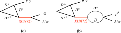
Figure 7: Triangle diagrams utilized in $X(3872)$ mass determination method. The diagrams include: (a) isospin-conserving $X(3872)\to J/\psi\omega$ ($\omega\to\pi^{+}\pi^{-}\pi^{0}$); (b) isospin-violating $X(3872)\to J/\psi\rho^{0}(\rho^{0}\to\pi^{+}\pi^{-})$. The $D^{*}\bar{D}$ loop violates the isospin symmetry due to the mass difference between the charged and neutral $D^{(*)}$.

As stated in the Introduction, a method has been proposed recently to determine the $X(3872)$ mass by analyzing TS peaks in the $X(3872)\pi$ or $X(3872)\gamma$ invariant mass (corresponding $W$) distributions guo_x3872 ; sakai_x3872 ; sakai2_x3872 . The TSs arise from diagrams as shown in Fig. 7 which are very similar to the diagram A. Thus, in the following, we speculate a possible impact of our result, Figs. 3(c), 5(b), and Table 1 in particular, on this method in a qualitative manner. Our result indicates that the TS peak from the diagram A would be a perfect fake of $X(3872)$ in the TS region of interest, and one needs to find a way to extract the $W$-lineshapes from data by separating off the fake from $X(3872)$(-like) signal events.

One may wonder if the non-resonant diagram A would give a negligible contribution compared with those from the $X(3872)$-pole. Because $X(3872)$ signal events are reconstructed from its decay products, whether or not an isospin violation, and a significant suppression associated with it, occurs in the decay is a key to answer this question. We first note that the non-resonant diagram A includes the $D^{*0}\bar{D}^{0}$ pair with the maximal mixture of isospin 0 and 1 components. Thus both $D^{*0}\bar{D}^{0}\to J/\psi\rho^{0}$ as in the diagram A and $D^{*0}\bar{D}^{0}\to J/\psi\omega$ proceed as isospin conserving processes. If the isospin is conserved in a resonant process as in Fig. 7(a), then the TS peak in the $W$-lineshape would be almost saturated by this process. The non-resonant diagram A, with $\rho^{0}$ replaced by $\omega$, may be negligible. However, if $X(3872)$ singnals are from isospin-violating decay products such as the process shown in Fig. 7(b), the resonant process would be significantly suppressed and the diagram A could be relevant. The degree of the suppression is uncertain, and could be estimated only model-dependently. Although some analysis such as Ref. prd2012_hanhart (Table I therein) seems to indicate that the amplitude magnitude of Fig. 7(b) is $\sim 1/4$ of that of Fig. 7(a), this does not necessarily means that the suppression due to the isospin violation is rather moderate $\sim 1/4$. It may also be the case that the $X(3872)\to J/\psi\omega$ coupling is weak and the suppression is large.

Thus, for measuring the $X(3872)\pi$ and $X(3872)\gamma$ lineshapes, one may be tempted to utilize a process that involves an isospin-conserving $X(3872)$ decay, thereby avoiding the concern about the non-resonant contributions. However, the experimentally cleanest signal of $X(3872)$ is obtained from the isospin-violating $X(3872)\to J/\psi\pi^{+}\pi^{-}$ decay, and this is the best channel to measure the $X(3872)\pi$ and $X(3872)\gamma$ lineshapes. Therefore, subtracting the background due to the non-resonant TS process like the diagram A is a practical issue.

An interesting idea to set a constraint on the non-resonant diagram A is to analyze the charge analogous $B^{0}\to(J/\psi\pi^{0}\pi^{-})K^{+}\pi^{0}$ process. As discussed in the previous section, the diagrams C and D creates an $X^{-}(3876)$-like sharp peak of width of $\sim 2$ MeV, and no similar resonance(-like) peak has been experimentally observed in the other processes. Therefore, if a peak as shown in Fig. 6 is found in $B^{0}\to(J/\psi\pi^{0}\pi^{-})K^{+}\pi^{0}$ data, this peak is likely to be from TSs of the diagrams C and D. Thus the data can give an ideal constraint on the magnitude of the diagrams C and D and, as a consequence, the diagrams A and B are also constrained. With the well-controlled triangle diagrams A and B, we can extract the $X(3872)$-pole amplitude and the corresponding $W$-lineshape in the TS region from $B^{0}\to(J/\psi\pi^{+}\pi^{-})K^{+}\pi^{-}$ data. The $X(3872)$ mass can now be assessed with a good control of the background.

References guo_x3872 ; sakai_x3872 ; sakai2_x3872 proposed to utilize diagrams in which internal particles $D^{*0}\bar{D}^{*0}D^{0}$ form the triangle. The charge analogous diagrams including this triangle do not satisfy the TS condition because $D^{*0}\to D^{+}\pi^{-}$ is forbidden at on-shell. Therefore, the corresponding non-resonant TS mechanism cannot be studied with the charge analogous process. However, once the relative strength and phase between the resonant and non-resonant TS mechanisms for $B^{0}\to(J/\psi\pi^{+}\pi^{-})K^{+}\pi^{-}$ are understood through the procedure described above, they can be brought to other triangle diagrams studied in Refs. guo_x3872 ; sakai_x3872 ; sakai2_x3872 . Some necessary corrections can be estimated reliably because they are associated with kinematical differences.

IV Summary

We have demonstrated that the triangle singularity (TS) inherent in the triangle diagram of Fig. 1(A) creates a sharp peak in the $J/\psi\pi^{+}\pi^{-}$ invariant mass distribution of $B^{0}\to J/\psi\pi^{+}\pi^{-}K^{+}\pi^{-}$. The Breit-Wigner fit of the peak in and near the TS region results in the mass $3871.68\pm 0.00$ MeV and width $0.42\pm 0.01$ MeV which are in perfect agreement with those of $X(3872)$, $3871.69\pm 0.17$ MeV and $<1.2$ MeV, from the precise measurements. The result is virtually independent of the uncertainty of the model parameters involved. This is because the TS, which does not depend on dynamical details, determines the peak position and the shape. However, this TS peak does not explain the $X(3872)$ peak observed in the Belle data for the same process. This is because the TS region is rather small in the whole phase-space and, combined with contributions from the other kinematical region, the total peak is significantly broader than the $X(3872)$-like TS peak.

We also studied a charge analogous $B^{0}\to(J/\psi\pi^{0}\pi^{-})K^{+}\pi^{0}$ process. We found that the triangle diagrams of Figs. 1(C) and 1(D) create an $X^{-}(3876)$-like TS peak with the width of $\sim 2$ MeV. We argued that this process is useful for studying and setting a constraint on the TS mechanisms because the TS contribution would not overlap with a resonant one.

We also argued that the TS peak from triangle diagrams like Figs. 1(A) could be a relevant background when extracting TS-enhanced $X(3872)\pi$ and $X(3872)\gamma$ lineshapes from data. It has been recently proposed that the $X(3872)$ mass can be determined by analyzing the lineshapes in the TS region. We suggested a procedure to separate the non-resonant and $X(3872)$-pole contributions in the TS region.

- (1) S. Godfrey and N. Isgur, Mesons in a relativized quark model with chromodynamics, Phys. Rev. D 32, 189 (1985).
- (2) S.K. Choi et al. (Belle Collaboration), Observation of a narrow charmoniumlike state in exclusive decays, Phys. Rev. Lett. 91, 262001 (2003).
- (3) E.S. Swanson, The New heavy mesons: A Status report, Phys. Rept. 429, 243 (2006).
- (4) M.B. Voloshin, Charmonium, Prog. Part. Nucl. Phys. 61, 455 (2008).
- (5) H.-X. Chen, W. Chen, X. Liu, and S.-L. Zhu, The hidden-charm pentaquark and tetraquark states, Phys. Rep. 639, 1 (2016).
- (6) A. Hosaka, T. Iijima, K. Miyabayashi, Y. Sakai, and S. Yasui, Exotic hadrons with heavy flavors: , , , and related states, PTEP 2016, 062C01 (2016).
- (7) R.F. Lebed, R.E. Mitchell, and E.S. Swanson, Heavy-Quark QCD Exotica, Prog. Part. Nucl. Phys. 93, 143 (2017).
- (8) A. Esposito, A. Pilloni, and A.D. Polosa, Multiquark Resonances, Phys. Rept. 668, 1 (2017).
- (9) A. Ali, J.S. Lange, and S. Stone, Exotics: Heavy Pentaquarks and Tetraquarks, Prog. Part. Nucl. Phys. 97, 123 (2017).
- (10) F.-K. Guo, C. Hanhart, U.-G. Meißner, Q. Wang, Q. Zhao, and B.-S. Zou, Hadronic molecules, Rev. Mod. Phys. 90, 015004 (2018).
- (11) S.L. Olsen, T. Skwarnicki, and D. Zieminska, Nonstandard heavy mesons and baryons: Experimental evidence, Rev. Mod. Phys. 90, 015003 (2018).
- (12) R.M. Albuquerque, J.M. Dias, K.P. Khemchandani, A. Martínez Torres, F.S. Navarra, M. Nielsen, and C.M. Zanetti, QCD sum rules approach to the , , and states, J. Phys. G 46, 093002 (2019).
- (13) B. Aubert et al. (BaBar Collaboration), Study of the decay and measurement of the branching fraction, Phys. Rev. D 71, 071103 (2005).
- (14) D. Acosta et al. (CDF II Collaboration), Observation of the narrow state in collisions at = 1.96 TeV, Phys. Rev. Lett. 93, 072001 (2004).
- (15) V.M. Abazov et al. (D0 Collaboration), Observation and properties of the decaying to in collisions at = 1.96 TeV, Phys. Rev. Lett. 93, 162002 (2004).
- (16) R. Aaij et al. (LHCb Collaboration), Observation of production in collisions at TeV, Eur. Phys. J. C 72, 1972 (2012).
- (17) M. Ablikim et al. (BESIII Collaboration), Observation of at BESIII, Phys. Rev. Lett. 112, 092001 (2014).
- (18) P. del Amo Sanchez et al. (BaBar Collaboration), Evidence for the decay , Phys. Rev. D 82, 011101(R) (2010).
- (19) M. Ablikim et al. (BESIII Collaboration), Study of and Observation of , Phys. Rev. Lett. 122, 232002 (2019).
- (20) V. Bhardwaj et al. (Belle Collaboration), Observation of and search for in decays, Phys. Rev. Lett. 107, 091803 (2011).
- (21) T. Aushev et al. (Belle Collaboration), Study of the decay, Phys. Rev. D 81, 031103(R) (2010).
- (22) E.S. Swanson, Short range structure in the , Phys. Lett. B 588, 189 (2004).
- (23) L. Zhao, L. Ma, and S.-L. Zhu, Spin-orbit force, recoil corrections, and possible and molecular states, Phys. Rev. D 89, 094026 (2014).
- (24) M. Suzuki, The boson: Molecule or charmonium, Phys. Rev. D 72, 114013 (2005).
- (25) Yu.S. Kalashnikova, Coupled-channel model for charmonium levels and an option for , Phys. Rev. D 72, 034010 (2005).
- (26) M. Takizawa and S. Takeuchi, as a hybrid state of charmonium and the hadronic molecule, PTEP 2013, 093D01 (2013).
- (27) S. Prelovsek and L. Leskovec, Evidence for from Scattering on the Lattice, Phys. Rev. Lett. 111, 192001 (2013).
- (28) M. Padmanath, C.B. Lang, and S. Prelovsek, and using diquark-antidiquark operators with lattice QCD, Phys. Rev. D 92, 034501 (2015).
- (29) L. Maiani, F. Piccinini, A.D. Polosa, and V. Riquer, Diquark-antidiquarks with hidden or open charm and the nature of , Phys. Rev. D 71, 014028 (2005).
- (30) W. Chen and S.-L. Zhu, The vector and axial-vector charmonium-like states, Phys. Rev. D 83, 034010 (2011).
- (31) L.D. Landau, On analytic properties of vertex parts in quantum field theory, Nucl. Phys. 13, 181 (1959).
- (32) S. Coleman and R.E. Norton, Singularities in the physical region, Nuovo Cim. 38, 438 (1965).
- (33) R. J. Eden, P. V. Landshoff, D. I. Olive and J. C. Polkinghorne, The Analytic S-Matrix, (Cambridge University Press, Cambridge, England, 1966).
- (34) M. Bayar, F. Aceti, F.-K. Guo, and E. Oset, A Discussion on Triangle Singularities in the Reaction, Phys. Rev. D 94, 074039 (2016).
- (35) Q. Wang, C. Hanhart, and Q. Zhao, Decoding the riddle of and , Phys. Rev. Lett. 111, 132003 (2013).
- (36) X.-H. Liu and G. Li, Exploring the threshold behavior and implications on the nature of and , Phys. Rev. D 88, 014013 (2013).
- (37) A.P. Szczepaniak, Triangle Singularities and Quarkonium Peaks, Phys. Lett. B 747, 410 (2015).
- (38) X.-H. Liu, M. Oka, and Q. Zhao, Searching for observable effects induced by anomalous triangle singularities, Phys. Lett. B 753, 297 (2016).
- (39) X.-H. Liu and G. Li, Could the observation of be a result of the near threshold rescattering effects?, Eur. Phys. J. C 76, 455 (2016).
- (40) X.-H. Liu, How to understand the underlying structures of , , and , Phys. Lett. B 766, 117 (2017).
- (41) A. Pilloni, C. Fernandez-Ramirez, A. Jackura, V. Mathieu, M. Mikhasenko, J. Nys, and A.P. Szczepaniak, Amplitude analysis and the nature of the , Phys. Lett. B 772, 200 (2017).
- (42) Q.-R. Gong, J.-L. Pang, Y.-F. Wang, and H.-Q. Zheng, The peak does not come from the “triangle singularity”, Eur. Phys. J. C 78, 276 (2018).
- (43) S.X. Nakamura and K. Tsushima, and as triangle singularities, Phys. Rev. D 100, 051502(R) (2019).
- (44) S.X. Nakamura, Triangle singularities in relevant to and , Phys. Rev. D 100, 011504(R) (2019).
- (45) F.-K. Guo, X.-H. Liu, and S. Sakai, Threshold cusps and triangle singularities in hadronic reactions, arXiv:1912.07030 [hep-ph].
- (46) A. Bala et al. (Belle Collaboration), Observation of in decays, Phys. Rev. D 91, 051101(R) (2015).
- (47) I. Adachi et al. (Belle Collaboration), Study of in meson decays, arXiv:0809.1224 [hep-ex].
- (48) F.-K. Guo, Novel Method for Precisely Measuring the Mass, Phys. Rev. Lett. 122, 202002 (2019).
- (49) S. Sakai, E. Oset, and F.-K. Guo, Triangle singularity in the reaction and sensitivity to the mass, Phys. Rev. D 101, 054030 (2020).
- (50) S. Sakai, H.-J. Jing, and F.-K. Guo, Possible precise measurements of the mass with the and , arXiv:2008.10829 [hep-ph].
- (51) E. Braaten, L.-P. He, and K. Ingles, Triangle Singularity in the Production of and a Photon in Annihilation, Phys. Rev. D 100, 031501(R) (2019).
- (52) E. Braaten, L.-P. He, and K. Ingles, Production of Accompanied by a Pion in Meson Decay, Phys. Rev. D 100, 074028 (2019).
- (53) E. Braaten, L.-P. He, and K. Ingles, Production of Accompanied by a Soft Pion at Hadron Colliders, Phys. Rev. D 100, 094006 (2019).
- (54) M. Tanabashi et al. (Particle Data Group), Review of Particle Physics, Phys. Rev. D 98, 030001 (2018).
- (55) J.L. Rosner, Hadronic and radiative widths, Phys. Rev. D 88, 034034 (2013).
- (56) P. Pakhlov et al. (Belle Collaboration), Production of New Charmoniumlike States in at GeV, Phys. Rev. Lett. 100, 202001 (2008).
- (57) M. Ablikim et al. (BESIII Collaboration), Observation of a charged charmoniumlike structure in at GeV, Phys. Rev. Lett. 112, 132001 (2014).
- (58) P. del Amo Sanchez (BaBar Collaboration), Measurement of the branching fractions, Phys. Rev. D 83, 032004 (2011).
- (59) H. Kamano, S.X. Nakamura, T.-S.H. Lee, and T. Sato, Unitary coupled-channels model for three-mesons decays of heavy mesons, Phys. Rev. D 84, 114019 (2011).
- (60) C. Hanhart, Yu.S. Kalashnikova, A.E. Kudryavtsev, and A.V. Nefediev, Remarks on the quantum numbers of from the invariant mass distributions of the and final states, Phys. Rev. D 85, 011501(R) (2012).