Stabilization of straight longitudinal dune under bimodal wind with large directional variation

Abstract

It has been observed that the direction in which a sand dune extends its crest line depends on seasonal variation of wind direction; when the variation is small, the crest line develops more or less perpendicularly to the mean wind direction to form a transverse dune with some undulation. In the case of bimodal wind with a large relative angle, however, the dune extends its crest along the mean wind direction and evolves into an almost straight longitudinal dune. Motivated by these observations, we investigate the dynamical stability of isolated dunes using the crest line model, where the dune dynamics is represented by its crest line motion. First, we extend the previous linear stability analysis under the unidirectional wind to the case with non-zero slant angle between the wind direction and the normal direction of the crest line, and show that the stability diagram does not depend on the slant angle. Secondly, we examine how the linear stability is affected by the seasonal changes of wind direction in the case of bimodal wind with equal strength and duration. For the transverse dune, we find that the stability is virtually the same with that for the unidirectional wind as long as the dune evolution during a season is small. On the other hand, in the case of the longitudinal dune, the dispersions of the growth rates for the perturbation are drastically different from those of the unidirectional wind, and we find that the largest growth rate is always located at $k=0$. This is because the growth of the perturbation with $k\neq 0$ is canceled by the alternating wind from opposite sides of the crest line even though it grows during each duration period of the bimodal wind. For a realistic parameter set, the system is in the wavy unstable regime of the stability diagram for the unidirectional wind, thus the straight transverse dune is unstable to develop undulation and eventually evolves into a string of barchans when the seasonal variation of wind direction is small, but the straight longitudinal dune is stabilized under the large variation of bimodal wind direction. We also perform numerical simulations on the crest line model, and find that the results are consistent with our linear analysis and the previous reports that show that the longitudinal dunes tend to have straight ridge and elongate over time.

I Introduction

Aeolian sand dunes are natural patterns ubiquitous on EarthBagnold (1941); Pye and Tsoar (1990); Cooke et al. (1993); Lancaster (1995) and even on other planets and satellites Warren (2013); Telfer et al. (2018). Their time evolution involves several processes of sand transport; successive ballistic motion of sand due to wind, called saltaion, provides the main contribution to the windward (stoss) side transport, while avalanche is dominant on the downwindward (leeward) side because the saltation is suppressed by the eddies formed at the crest line, where the wind flow separates from the sand bed. Lateral transport perpendicular to the wind arises from reptation i.e. stochastic motion of the grains ejected by collisions of saltation grains on the sand bed.

A flat sand bed under unidirectional wind destabilizes in favor of sand wave due to the primary instability, which is now well understood as a result of the phase lag between the flow shear stress and the bed-form. The minimum size of a dune is determined by the wavelength of the most unstable mode, which has been found to correspond with the saturation length, i.e., the length needed for the sediment to equilibrate with the flowAndreotti et al. (2002a, b); Kroy et al. (2002a, b); Sauermann et al. (2001). Under unsteady wind with varying strength and direction, the secondary instabilities occur to develop a variety of three-dimensional patterns, such as crescentic barchans, star and linear dunes with complex and compound patterns with a variety of length scales and orientationsCourrech du Pont et al. (2014). Such instabilities are still mostly unexplored systematically.

From field observations, it has been noticed that under seasonal bimodal wind with comparable strength and small diversity angle, sand bed develops into transverse dunes with some undulation; its crest lines extend perpendicular to the mean wind direction. On the other hand, when the diversity angle of the bimodal winds is sufficiently large, i.e. larger than 90 degrees, sand bed forms longitudinal dunes, whose crest lines extend along the mean wind directionBagnold (1941); Lancaster (1995). Such transition from the transverse to the longitudinal dune has been also confirmed by experimentsRubin and Hunter (1987); Courrech du Pont et al. (2014); Rubin and Ikeda (1990); Taniguchi et al. (2012); Reffet et al. (2010) and simulationsParteli et al. (2009); Parteli and Herrmann (2007). Understanding the selection mechanism of emerging dune types by the pattern of the wind direction change has been recognized as one of fundamental issues of dune morphology.Bagnold (1941); Pye and Tsoar (1990); Cooke et al. (1993); Lancaster (1995); Warren (2013).

In addition to the wind direction, if the wind strength and the duration also vary in the bimodal wind, the relation between the wind pattern and the crest line direction of dune should become far more complicated. It is notable that such a relationship may be summarized by a simple empirical hypothesis called “the maximization of the gross sand transport normal to the crest” Rubin and Hunter (1987); Rubin and Ikeda (1990). The theoretical understanding of this hypothesis, however, has not been reached yet, and except for a few approachesWerner and Kocurek (1997); Gadal et al. (2019), little has been worked out theoretically to clarify how the dune direction is determined under the unsteady wind. The difficulty is that most of theoretical descriptions of dune evolution are based on complex formulation to describe mixed effects of fluid and granular dynamics, thus analytical treatment is not feasible even for boldly simplified numerical models like cell modelsWerner (1995); Nishimori and Ouchi (1993); Nishimori et al. (1998).

An exception is the crest line model, which describes the dune evolution by a couple of partial-differential equations for the position and height of the crest line of the duneGuignier et al. (2013). Its dynamics is based on simple assumptions for the longitudinal and the lateral transportations of sands. Despite its simplicity, it has been demonstrated that the model is capable to reproduce basic feature of the dune dynamics with its instabilityGuignier et al. (2013). In this paper, using the crest line model, we present theoretical analysis and numerical simulations for the stability of dune dynamics under bimodal winds with equal strength and duration in the case of the non-zero slant angle $\chi$, i.e. in the case where the wind direction is not normal to the crest line.

The paper is organized as follows. After introducing the crest line model in Sec.2, the linear stability of the straight crest with the non-zero slant angle $\chi$ is presented in Sec.3 to show that the stability diagram does not depend on $\chi$. Then in Sec.4, the formalism of the linear stability analysis is extended to the case for the bimodal wind with the equal wind strength and the equal duration. The expressions for the growth rate of perturbation are obtained for the case of the transverse dune, and for the case of the longitudinal dune. In Sec.5, these growth rates are numerically estimated as a function of the wave number $k$ for various slant angle $\chi$ and parameter sets, and in Sec.6, numerical simulations are presented for the crest line model to compare with the results of the linear stability analysis. The concluding remarks are given in Sec.7.

II Crest line model

The crest line model is originally introduced by Guignier et al.Guignier et al. (2013) to describe dune dynamics under unidirectional steady wind. A dune on a non-erodible bed is represented by its crest line with its stream-wise position $x$ and height $h$ as a function of $y$, the position along the co-ordinate axis perpendicular to the streamline (Fig.1(a)). Following the study of Niiya et al.Niiya et al. (2010, 2012), the key hypothesis for simplification in this model is that any stream-wise cross-section of dune should be similar triangle. Then, the dune configuration at the time $t$ is uniquely defined by the position $x(y,t)$ and the height $h(y,t)$ of the crest with the angles of the windward and downwindward slopes, $\theta$ and $\phi$.

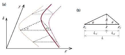
Figure 1: Co-ordinate system for the crest line model and similar triangle of dune cross section. (a) The $x$-axis is taken to be parallel to the wind direction and the $y$-axis is perpendicular to it; the $h$-axis is vertical. The crest line of the sand dune is shown by the thick brown line, which is represented by $(x(y),y,h(y))$. cross section of the dune by a plane parallel to the $x$-$h$ plane is similar triangle, whose peak is at the crest line. The remaining two vertices on the base of the triangle are the windward and downwindward ends of the dune, which are shown by the thin brown lines, $(x_{u}(y),y)$ and $(x_{d}(y),y)$ in the $x$-$y$ plane. (b) The height and the length of the base of the triangle are $h$ and $L$. $L_{u}$ and $L_{d}$ are the lengths of the windward and the downwindward parts of the base.

It is convenient to introduce the positions of the windward and the downwindward ends of the slope, $x_{u}$ and $x_{d}$, respectively, which are given by

$$x_{u}=x-{B\over A}h,\qquad x_{d}=x+{C\over A}h.$$ (1)

The parameters $A$, $B$, and $C$ are the geometrical parameters defined as

$$A\equiv\frac{h}{L},\quad B\equiv\frac{L_{u}}{L},\quad C\equiv\frac{L_{d}}{L},$$ (2)

where $L$, $L_{u}$, and $L_{d}$ are the total, the windward side, and the downwindward side lengths of the dune, respectively (Fig.1(b)). Note that the simple equality

$$B+C=1$$ (3)

holds because $L=L_{u}+L_{d}$.

Figure 2: Change of the cross section caused by small advance of the sand dune. The total change of the cross section consists of the decrement $h\,dx_{u}$ in the windward side and the increment $h\,dx_{d}$ in the downwindward side.

The time development of the crest line is determined by the sand transport in the $x$ and the $y$ directions, i.e. the longitudinal transport and the lateral transport. The longitudinal transport caused by wind consists of the incoming sand flux density $f_{\rm in}$ and the outgoing flux density over the crest line $q$. Both depend on the flow strength, and are determined by the upwind boundary. A fraction of the sand flux $q$ over the crest line is captured on the downwind slope; that fraction is called as the efficiency rate $T_{e}$Cooke et al. (1993); Momiji and Warren (2000) and shown to be an increasing function of the dune height $h$ for a given wind strengthMomiji and Warren (2000).

The lateral transport is caused by random motion of sand grains biased by lateral gradient of the dune face. Thus, the local lateral flux densities are assumed to be proportional to the gradients of the dune faces in the transverse direction with the diffusion coefficients $D_{u}$ and $D_{d}$ of the upwind and the downwind slope, respectively. Then the total lateral fluxes on the windward and the downwindward slopes, $J_{u}$ and $J_{d}$, integrated over each dune face along the longitudinal direction are shown to be

$$J_{u} = D_{u}\,h{\partial x_{u}\over\partial y},$$ (4)

$$J_{d} = -D_{d}\,h{\partial x_{d}\over\partial y}.$$ (5)

The change of the cross section by the displacement of the upstream slope is $-hdx_{u}$ and that by that of the downstream slope is $hdx_{d}$ (Fig.2). By balancing these changes with the influxes of grain through the corresponding slopes of the dune, we obtain the time evolution equations

$$-h{\partial x_{u}\over\partial t} =f_{\rm in}-q-{\partial J_{u}\over\partial y},$$ (6)

$$h{\partial x_{d}\over\partial t} =T_{e}q-{\partial J_{d}\over\partial y}.$$ (7)

Using Eqs.(1), these equations lead to the time evolution for $x$ and $h$,

$${1\over A}\,h\frac{\partial h}{\partial t} = f_{\rm in}-(1-T_{e})q-\frac{\partial J_{d}}{\partial y}-\frac{\partial J_{u}}{\partial y},$$ (8)

$$h\frac{\partial x}{\partial t} = q(BT_{e}+C)-Cf_{\rm in}-B\frac{\partial J_{d}}{\partial y}+C\frac{\partial J_{u}}{\partial y},$$ (9)

which are Eqs. (3) and (4) in ref.Guignier et al. (2013).

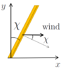
Figure 3: Straight dune with the slant angle $\chi$. The wind direction is shown by the thick arrow, which is slanted by the angle $\chi$ from the normal direction of the crest line.

Eqs. (8) and (9) have the steady uniform solution, i.e. the infinite rectilinear dune of the height $h_{0}$ migrating with the constant speed $V_{0}$ with the slant angle $\chi$,

$$x_{0}(y,t) = V_{0}t+y\tan\chi,$$ (10)

$$h_{0}(y,t) = h_{0},$$ (11)

as shown in Fig.3. Here, $h_{0}$ and $V_{0}$ are determined by

$$0 = f_{\rm in}-\Bigl{(}1-T_{e}(h_{0})\Bigr{)}\,q,$$ (12)

$$V_{0} = \frac{qT_{e}(h_{0})}{h_{0}}=\frac{q-f_{\rm in}}{h_{0}}.$$ (13)

The migration speed $V_{0}$ is inversely proportional to the height of the dune, but both $h_{0}$ and $V_{0}$ are independent of the slant angle $\chi$. This comes from the fact that $q$ and $T_{e}$ are taken to be independent of $\chi$ or $\partial x/\partial y$, which should be reasonable approximation for small $\chi$ because of the $\chi\leftrightarrow-\chi$ symmetry of the problem, but may not be valid for large value of $\chi$. Note that the migration speed $V_{0}$ by Eq.(13) is the speed along the wind direction, thus the speed normal the crest line is given by $V_{0}\cos\chi$, which is smaller than $V_{0}$.

For numerical simulations in Sec.VI, we take $f_{\rm in}=0$ and assume that $T_{e}$ and $q$ depend on $h$ as

$$T_{e}(h) =\left\{\begin{array}[]{ll}h/h_{c}&\mbox{for $0\leq h\leq h_{c}$}\\ 1&\mbox{for $h>h_{c}$}\end{array}\right.$$ (16)

$$q(h) =\left\{\begin{array}[]{ll}q_{c}\;h/h_{c}&\mbox{for $0\leq h\leq h_{c}$}\\ q_{c}&\mbox{for $h>h_{c}$}\end{array}\right.$$ (19)

with a critical height $h_{c}$. The form $T_{e}(h)$ of Eq.(16) is employed by Ref. Guignier et al. (2013) as the simplest form for a monotonically increasing function with the saturation value 1, which means that dunes can be self-sustained without the influx $f_{\rm in}$ if it is large enough. We introduce the form $q(h)$ of Eq.(19) here because $q$ should be zero in the $h\to 0$ limit when $f_{\rm in}=0$. The critical heights $h_{c}$ for these quantities are not necessarily the same, but would be of the same order related to the saturation length of the sand transport. We take them the same for simplicity.

III Linear Stability of rectilinear dunes for non-zero $\chi$

In this section, we present the linear stability analysis of the steady uniform solution Eqs.(10) and (11) for non-zero value of $\chi$. As for the case with $\chi=0$, i.e. the case of the transverse dune with the crest line perpendicular to the wind, the stability analysis has been worked out by Guignier et al. Guignier et al. (2013), and the stability has been determined in terms of two dimensionless parameters,

$$\delta=\frac{h_{0}T_{e}^{\prime}(h_{0})}{T_{e}(h_{0})},\qquad\rho=\frac{D_{d}}{D_{u}}.$$ (20)

The positive $\delta$ destabilizes the steady solution because the higher dune height $h$ increases the sand deposit on the downwind slope $qT_{e}(h)$, which makes the dune height even higher. The larger $\rho$ also destabilizes it because the lateral diffusion in the downwindward slope accumulates the sand in the concave crest line region, which further delay the advance of the crest line, while the lateral diffusion in the windward slope has the opposite effect. They obtained the stability diagram in the $\delta-\rho$ plane.

We extend the linear stability analysis to the case with the non-zero $\chi$ and the case under the bimodal winds with the same strength and duration.

III.1 Linear analysis

The stability of the steady solution Eqs.(10) and (11) are examined by the sinusoidal perturbation of the wave number $k$ with the coefficient $x_{k}(t)$ and $h_{k}(t)$,

$$x(y,t) = x_{0}(y,t)+x_{k}(t)e^{iky},$$ (21)

$$h(y,t) = h_{0}+h_{k}(t)e^{iky}.$$ (22)

Note that $k$ is the wave number not along the crest line but along the $y$-axis. Substituting Eqs. (21) and (22) into Eqs. (8) and (9), within the linear approximation we obtain

$${d\over dt}\left|\bm{x}_{k}(t)\right>=\hat{A}_{k}(\chi)\left|\bm{x}_{k}(t)\right>$$ (23)

with the ket vector

$$\left|\bm{x}_{k}(t)\right>\equiv\left(\begin{array}[]{c}x_{k}(t)\\ h_{k}(t)\end{array}\right),$$ (24)

and the matrix $\hat{A}_{k}(\chi)$ given by

$$\hat{A}_{k}(\chi)\equiv \left(\begin{array}[]{cc}-(BD_{d}+CD_{u})k^{2},&\displaystyle{qBT_{e}^{\prime}-V_{0}\over h_{0}}+{BD_{d}+CD_{u}\over h_{0}}\,ik\tan\chi-{BC\over A}(D_{d}-D_{u})k^{2}\\ -A(D_{d}-D_{u})k^{2},&\displaystyle{AqT_{e}^{\prime}\over h_{0}}+{A(D_{d}-D_{u})\over h_{0}}\,ik\tan\chi-(CD_{d}+BD_{u})k^{2}\end{array}\right).$$ (27)

For later use, we introduce the notation for the eigenvalues $\omega_{k}^{\pm}(\chi)$ (${\rm Re}\,\omega_{k}^{+}(\chi)>{\rm Re}\,\omega_{k}^{-}(\chi)$) and the corresponding left and right eigenvectors $\left<\bm{x}_{k}^{\pm}(\chi)\right|$ and $\left|\bm{x}_{k}^{\pm}(\chi)\right>$, respectively, with the ortho-normalization conditions

$$\left<\bm{x}_{k}^{\pm}(\chi)|\bm{x}_{k}^{\pm}(\chi)\right>=1,\quad\left<\bm{x}_{k}^{\pm}(\chi)|\bm{x}_{k}^{\mp}(\chi)\right>=0.$$ (28)

The eigenvalues $\omega_{k}^{\pm}(\chi)$ are determined by the characteristic equation,

$$\omega^{2}-\omega\left[F(k)+{A\over h_{0}}(D_{d}-D_{u})ik\tan\chi\right]+G(k)k^{2}=0,$$ (29)

as

$$\omega_{k}^{\pm}(\chi) ={1\over 2}\left(F(k)+{A\over h_{0}}\big{(}D_{d}-D_{u}\big{)}ik\tan\chi\pm\sqrt{\left(F(k)+{A\over h_{0}}\big{(}D_{d}-D_{u}\big{)}ik\tan\chi\right)^{2}-4G(k)k^{2}}\;\right)$$ (30)

with the functions $F(k)$ and $G(k)$ defined by

$$F(k) \equiv{AqT_{e}^{\prime}\over h_{0}}-(D_{d}+D_{u})k^{2},$$ (31)

$$G(k) \equiv-{A\over h_{0}}\big{(}D_{u}qT_{e}^{\prime}+V_{0}(D_{d}-D_{u})\big{)}+D_{d}D_{u}k^{2}.$$ (32)

Note that Eqs.(29)$\sim$(32) do not depend on $B$ and $C$ even though Eq.(27) depends on them.

III.2 Stability diagram for unidirectional wind with non-zero $\chi$

In the case of unidirectional wind, we demonstrate that the stability diagram for $\chi\neq 0$ is the same as that for $\chi=0$ as is shown in Fig. 4. For the the uniform perturbation with $k=0$, it is easy to see that the stability is the same with the case of $\chi=0$ because the $\chi$ term always appears in combination with the wave number $ik$. In this case, the characteristic equation (29) has the solutions

$$\omega={AqT_{e}^{\prime}\over h_{0}},\quad 0,$$ (33)

therefore the uniform solution given by (10) and (11) is unstable for $T_{e}^{\prime}>0$ (or $\delta>0$) and marginally stable for $T_{e}^{\prime}\leq 0$ (or $\delta\leq 0$).

The stability against the $k\neq 0$ perturbation can be determined by examining the dispersion of the unstable mode of Eq.(33) for $T_{e}^{\prime}>0$, or the marginally stable mode of Eq.(33) for $T_{e}^{\prime}<0$. In the region $\delta>0$ ($T_{e}^{\prime}>0$), the dispersion of the unstable mode is expanded as

$$\omega={AqT_{e}^{\prime}\over h_{0}}+{A\over h_{0}}(D_{d}-D_{u})ik\tan\chi+\left({V_{0}\over qT_{e}^{\prime}}(D_{d}-D_{u})-D_{d}\right)k^{2}+O(k^{3}),$$ (34)

for small $k$, thus the $k\neq 0$ mode is even more unstable than that of $k=0$ if

$$D_{d}>{D_{u}\over 1-qT_{e}^{\prime}/V_{0}}\quad\mbox{or}\quad\rho>{1\over 1-\delta}.$$ (35)

The dispersion for the marginal mode in the $\delta<0$ ($T_{e}^{\prime}<0$) region is expanded as

$$\omega=-\left(D_{u}+{V_{0}\over qT_{e}^{\prime}}(D_{d}-D_{u})\right)k^{2}+O(k^{3}),$$ (36)

for small $k$, thus the $k\neq 0$ mode is unstable for

$$D_{d}>D_{u}\left(1-{qT_{e}^{\prime}\over V_{0}}\right)\quad\mbox{or}\quad\rho>1-\delta.$$ (37)

All of these stability conditions, Eqs.(33), (35), and (37), do not depend on the angle $\chi$, therefore, the stability diagram given by Fig.4 for the uniform solution is the same with the case of $\chi=0$.

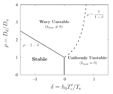
Figure 4: Stability diagram for both $\chi=0$ and $\chi\neq 0$ cases.

There are three regimes of stability: (i) stable regime, i.e. the steady solution is linearly stable for any $k$, (ii) uniformly unstable regime, i.e. there exists a band of unstable modes with the most unstable mode at $k_{\rm max}=0$, and (iii) wavy unstable regime, i.e. there exists a band of unstable modes with the most unstable mode at $k_{\rm max}\neq 0$. Although the boundaries of these regimes do not depend on $\chi$, the wave number $k_{\rm max}$ of the most unstable mode depends on $\chi$ in the wavy unstable regime.

In the real aeolian sand dunes, avalanches in the downwindward slope dominate the lateral sand transport, which suggests $\rho\gg 1$. By a numerical estimation using field data, Momiji et al. Momiji and Warren (2000) showed that the efficiency rate $T_{e}$ for aeolian dunes is an increasing function of the dune height ($\delta>0$). The parameters of the real aeolian sand dunes, therefore, are presumed to be in the wavy unstable regime.

IV Linear stability of rectilinear dune under bimodal winds

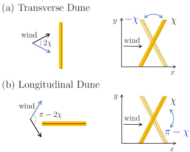
Figure 5: Transverse dune (a) and longitudinal dune (b) under bimodal wind. The wind directions are shown by the black and blue arrows. In the crest line model, the $x$-axis is taken parallel to the wind direction, therefore, every time the wind changes its direction, the crest line need to be rotated between the two slant angles, i.e. $\chi$ and $-\chi$ for the transverse dune, and $\chi$ and $\pi-\chi$ for the longitudinal dune.

Now, we extend the above stability analysis to the bimodal wind case, where the wind direction changes alternately. We consider the two cases: (A) the case of transverse dune, where the wind direction switches between $\chi$ and $-\chi$, and (B) the case of longitudinal dune, where the wind direction changes between $\chi$ and $\pi-\chi$ (Fig.5). The angles between the bimodal winds are $2\chi$ for the transverse dune and $\pi-2\chi$ for the longitudinal dune. The wind is supposed to blow in each direction for the same duration time $T$. We also assume that the geometrical parameters $A$, $B$, and $C$ relax quickly to the original steady values after the wind direction switches even in the case where the windward and the downwindward sides are interchanged. This is not necessarily true in the usual situation, where the migration distance during the duration time of each wind is shorter than the width of the dune. In such a situation, the geometrical parameters, $A$, $B$, and $C$ should relax to some averaged values over many periods.

IV.1 Transverse dune

First, we consider the transverse dune under the bimodal wind with the direction $\chi$ and $-\chi$. In our formalism (9) and (8), the wind is always supposed to be in the $x$-direction and the uniform solution (10) and (11) is inclined by the angle $\chi$, thus we rotate the solution by $\pm 2\chi$ as in Fig.5(a) when the wind direction switches, which corresponds that the co-ordinate system is rotated by $\mp 2\chi$.

Suppose that the wind blows in the $\chi$ direction for $0<t<T$, then the time evolution of the perturbation is governed by Eq.(23) and the solution is given by

$$\left|\bm{x}_{k}(t)\right>=e^{\hat{A}_{k}(\chi)t}\left|\bm{x}_{k}(0)\right>.$$ (38)

At $t=T$, the wind direction changes from $\chi$ to $-\chi$. We change the zero-th order solution (10) and (11) by replacing $\chi$ by $-\chi$, but the perturbation $x_{k}$ and $h_{k}$ remain the same. Thus the perturbation evolve for $T<t<2T$ as

$$\left|\bm{x}_{k}(t)\right>=e^{\hat{A}_{k}(-\chi)(t-T)}e^{\hat{A}_{k}(\chi)T}\left|\bm{x}_{k}(0)\right>,$$ (39)

therefore, after one cycle of the bimodal wind at $t=2T$, the perturbation evolves as

$$\left|\bm{x}_{k}(2T)\right>=\hat{\Lambda}_{\rm trans}\left|\bm{x}_{k}(0)\right>$$ (40)

with the evolution matrix

$$\hat{\Lambda}_{\rm trans}\equiv e^{\hat{A}_{k}(-\chi)T}e^{\hat{A}_{k}(\chi)T}=\left(e^{\hat{A}_{k}(\chi)T}\right)^{*}\,e^{\hat{A}_{k}(\chi)T}.$$ (41)

The stability of the transverse dune under the bimodal wind can be determined by the eigenvalues $\lambda_{\rm trans}^{\pm}$ of the matrix $\hat{\Lambda}_{\rm trans}$. We define

$$\bar{\omega}_{\rm trans}^{\pm}\equiv{\log\lambda_{\rm trans}^{\pm}\over 2T},$$ (42)

then the average growth rate over the one period of the bimodal wind is given by ${\rm Re\,}[\bar{\omega}_{\rm trans}^{\pm}]$.

IV.2 Longitudinal dune

In the case of longitudinal dune, the analysis can be performed almost in the same way as in the case of the transverse dune, but the difference is that the windward and the downwindward sides are interchanged when the wind direction changes between $\chi$ and $\pi-\chi$, thus $x_{k}$ should be replaced by $-x_{k}$ while $h_{k}$ remains the same. This can be represented by

$$-\hat{\sigma}_{z}\left|\bm{x}_{k}\right>$$ (43)

with the spin matrix

$$\hat{\sigma}_{z}=\left(\begin{array}[]{cc}1,&0\\ 0,&-1\end{array}\right).$$ (44)

At the same time, the sign of wave number of the perturbation is also inverted because the direction of the $y$ axis flips as can be seen in Fig.5(b). Thus, the time evolution matrix for the one period of the bimodal wind is given by

$$\hat{\Lambda}_{\rm long}\equiv(-\hat{\sigma}_{z})e^{\hat{A}_{-k}(\pi-\chi)T}(-\hat{\sigma}_{z})e^{\hat{A}_{k}(\chi)T}=\left(\hat{\sigma}_{z}\,e^{\hat{A}_{k}(\chi)T}\right)^{2}$$ (45)

and the stability is determined by its eigenvalues $\lambda_{\rm long}^{\pm}$ or the average growth rate, i.e. the real part of $\bar{\omega}_{\rm long}^{\pm}$ defined as

$$\bar{\omega}_{\rm long}^{\pm}\equiv{\log\lambda_{\rm long}^{\pm}\over 2T}.$$ (46)

V Numerical estimate of growth rate

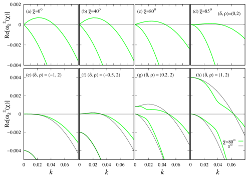
Figure 6: The dispersions of the growth rates ${\rm Re}\,[\omega_{k}^{\pm}(\chi)]$ of the perturbation under the unidirectional wind for some values of $\delta$ and the wind direction $\tilde{\chi}$ in the wavy unstable region with $\rho=2$. The parameters are $h_{0}=5$, $q=1$, $D_{u}=1$, $T_{e}(h_{0})=1$, $(A,B,C)=(0.1,0.8,0.2)$ with $T_{e}^{\prime}(h_{0})=(T_{e}(h_{0})/h_{0})\delta$ and $D_{d}=D_{u}\rho$.

We numerically estimate the average growth rates of the sinusoidal perturbation to the uniform solution with non-zero slant angle. To represent numerical values, we employ the unit system where

$$h_{c}=q_{c}=D_{u}=1;$$ (47)

$h_{c}$ and $q_{c}$ are the critical height and the saturated flux, respectively, in Eqs.(16) and (19), that define the functions $T_{e}(h)$ and $q(h)$. We adopt the same unit for $h$ and $x$, then the numerical values for $h$, $x$, $y$, and $t$ should read as those for

$${h\over h_{c}},\quad{x\over h_{c}},\quad{y\over h_{c}\sqrt{D_{u}/q_{c}}},\quad{t\over{h_{c}^{2}/q_{c}}},$$ (48)

respectively. In this system, numerical values of the slant angle should be given by $\tilde{\chi}$ defined by

$$\tan\tilde{\chi}\equiv\sqrt{D_{u}\over q_{c}}\,\tan\chi$$ (49)

from the actual slant angle $\chi$ because the unit is different between the $x$ and $y$ direction.

Considering the case of saturated self-sustained dune

$$f_{\rm in}=0,\quad T_{e}(h_{0})=1,\quad q=q_{c},$$ (50)

the perturbation is examined around the uniform solution (10) and (11) with

$$h_{0}=5h_{c},\quad V_{0}={q_{c}\over 5h_{c}}.$$ (51)

We regard $\delta=h_{0}T_{e}^{\prime}(h_{0})/T_{e}(h_{0})$ as a parameter in this section although $T_{e}^{\prime}(h_{0})$ is zero for $h_{0}=5h_{c}$ if we employ Eq.(16) for $T_{e}(h_{0})$.

V.1 Unidirectional wind

Fig. 6 shows the real parts of the eigenvalues $\omega_{k}^{\pm}(\chi)$ of the matrix $\hat{A}_{k}(\chi)$ given by Eq.(27). They correspond to the growth rate for the perturbation with the wave number $k$ under the unidirectional wind. Note that the wave number $k$ is defined along the $y$ axis; the wave number along the crest line $k_{\rm crest}$ is given by

$$k_{\rm crest}=k\cos\chi.$$ (52)

The upper plots of Fig.6 show the dispersion for various values of the angle $\chi$ at $(\delta,\rho)=(0,2)$, which is in the wavy unstable regime. The dispersion as a function $k$ changes significantly only for very large $\tilde{\chi}\gtrsim 80^{\circ}$, where the validity of the present model is not so clear. For the moderate value of $\tilde{\chi}\lesssim 40^{\circ}$, only visible difference would be the change in the wave number (52), i.e. the wave length of the most unstable mode along the crest line is elongated by the factor $\cos\chi$. As we will see below, this insensitivity of the dispersions on the slant angle $\chi$ is a common feature for all the cases we study in the following.

In order to see the effect of non-zero $\chi$ for other values of $(\delta,\rho)$, in the lower graphs the dispersions of the growth rate are plotted along the $\rho=2$ line in the wavy unstable region for $\tilde{\chi}=80^{\circ}$ together with those of $\tilde{\chi}=0$; Even for this unrealistically large value of $\tilde{\chi}=80^{\circ}$, the difference in the dispersions is modest. The dispersion of the unstable modes have maxima at finite $k$ for both $\tilde{\chi}=0$ and $80^{\circ}$ cases in the region of $-1<\delta<{1/2}$ with $\rho=2$ as expected from the stability diagram in Fig.4.

V.2 Transverse dune under bimodal wind

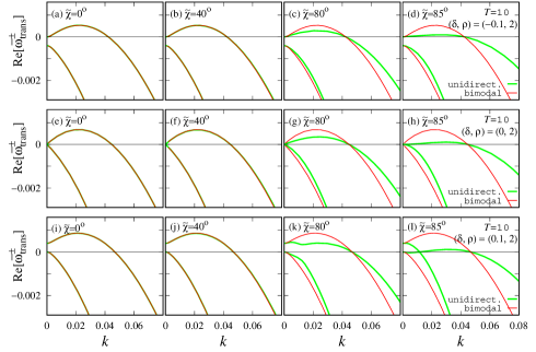
Figure 7: The dispersions of the average growth rate ${\rm Re}\,[\bar{\omega}^{\pm}_{\rm trans}]$ of the transverse dune under the bimodal wind with $T=10$ for various slant angle $\tilde{\chi}$ in the wavy unstable regime, $(\delta,\rho)=(-0.1,2)$ (upper), $(0,2)$ (middle), and $(0.1,2)$ (lower). The dispersions under the unidirectional wind are also shown for comparison. The parameters are $h_{0}=5$, $q=1$, $D_{u}=1$, $T_{e}(h_{0})=1$, $(A,B,C)=(0.1,0.8,0.2)$ with $T_{e}^{\prime}(h_{0})=(T_{e}(h_{0})/h_{0})\delta$ and $D_{d}=D_{u}\rho$.

Fig.7 shows the dispersions of the average growth rate Eq.(42) for the transverse dune under the bimodal wind for various slant angle $\tilde{\chi}$; the growth rates under the unidirectional wind, ${\rm Re}\,[\omega_{k}^{\pm}(\chi)]$, for the same slant angle $\tilde{\chi}$ are also shown for comparison. The wind duration of each direction $T$ is 10 in the unit of Eq.(47) and the model parameters are taken in the wavy unstable regime for the unidirectional wind, i.e. $(\delta,\rho)=(-0.1,2)$, (0,2), and (0.1,2), thus the wave number for the most unstable mode $k_{\rm max}$ is non-zero.

As a function of $k$, the dispersion for the bimodal wind (the red curves) hardly depends on the slant angle even for the very large $\tilde{\chi}\gtrsim 80^{\circ}$, where the dispersions for the unidirectional wind (the green curves) deviates significantly from that of $\tilde{\chi}=0$. This can be understood as follows; for small $T$ which satisfies ${\omega}^{\pm}_{k}(\chi)T\ll 1$, the evolution matrix $\hat{\Lambda}_{\rm trans}$ given by Eq.(41) can be approximated as

$$\hat{\Lambda}_{\rm trans}\approx 1+\hat{A}^{*}_{k}(\chi)T+\hat{A}_{k}(\chi)T=1+\hat{A}_{k}(0)2T,$$ (53)

thus

$${\bar{\omega}}_{\rm trans}^{\pm}(k;\chi)\approx\omega_{k}^{\pm}(0).$$ (54)

This means that the effects of the slant angle from the two winds with $\chi$ and $-\chi$ in Fig. 5 cancel each other after one period of the bimodal wind.

Fig.8 shows the duration time $T$ dependence of the dispersions for $\tilde{\chi}=80^{\circ}$ and $(\delta,\rho)=(0.1,2)$. For such a large value of slant angle, the dispersion for the bimodal wind with $T=10$ is still close to that of $\tilde{\chi}=0$, but significantly different from that for the unidirectional wind with the same value of $\tilde{\chi}=80^{\circ}$. For very large $T$, one can see that the dispersions for the bimodal wind become closer to those for the unidirectional wind as one should expect; the bimodal wind with very long $T$ should look like the unidirectional wind. We do not show the $T$-dependence for a smaller slant angle, e.g. $\tilde{\chi}\lesssim 40^{\circ}$, but the dispersions hardly depend on the duration of each wind $T$ because the dispersions for the bimodal wind and the unidirectional wind are already very close to each other and to those for the $\tilde{\chi}=0$ case.

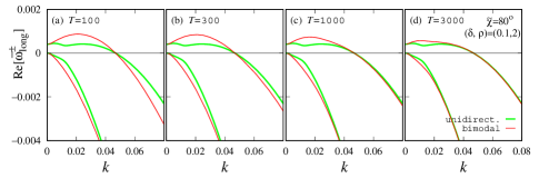
Figure 8: The dispersions of the average growth rate ${\rm Re}\,[\bar{\omega}^{\pm}_{\rm trans}]$ of the transverse dune under the bimodal wind for various $T$ with $\tilde{\chi}=80^{\circ}$ at $(\delta,\rho)=(0.1,2)$ along with those under the unidirectional wind for comparison. The parameters are $h_{0}=5$, $q=1$, $D_{u}=1$, $T_{e}(h_{0})=1$, $(A,B,C)=(0.1,0.8,0.2)$ with $T_{e}^{\prime}(h_{0})=(T_{e}(h_{0})/h_{0})\delta$ and $D_{d}=D_{u}\rho$.

V.3 Longitudinal dune under bimodal wind

Fig.9 shows the dispersions of the average growth rate given by Eq.(46) of the longitudinal dune under the bimodal wind for various slant angle $\tilde{\chi}$ with $T=10$ and $(\delta,\rho)=(-0.1,2)$, (0,2), and (0.1,2). It is remarkable that the wave number for the most unstable mode $k_{\rm max}$ is always zero for the longitudinal dune under the bimodal wind, even though the parameters $(\delta,\rho)$ are in the wavy unstable regime for the unidirectional wind.

This can be understood as follows; for ${\omega}^{\pm}_{k}(\chi)T\ll 1$, the evolution matrix $\hat{\Lambda}_{\rm long}$ of Eq.(45) can be approximated as

$$\hat{\Lambda}_{\rm long}\approx 1+\hat{\sigma}_{z}\hat{A}_{k}(\chi)\hat{\sigma}_{z}T+\hat{A}_{k}(\chi)T=1+\hat{A}_{k}^{\rm diag}(\chi)2T,$$ (55)

where, $\hat{A}_{k}^{\rm diag}(\chi)$ represents the diagonal part of $\hat{A}_{k}(\chi)$,

$$\hat{A}_{k}^{\rm diag}(\chi)\equiv\left(\begin{array}[]{cc}-(BD_{d}+CD_{u})k^{2},&0\\ 0,&AqT_{e}^{\prime}/h_{0}+A(D_{d}-D_{u})/h_{0}\,ik\tan\chi-(CD_{d}+BD_{u})k^{2}\end{array}\right).$$ (58)

Thus we have

$$\bar{\omega}_{\rm long}^{\pm}(k;\chi)\approx\left\{\begin{array}[]{l}-(BD_{d}+CD_{u})k^{2}\\ AqT_{e}^{\prime}/h_{0}+A(D_{d}-D_{u})/h_{0}\,ik\tan\chi-(CD_{d}+BD_{u})k^{2}\end{array}\right.,$$ (59)

where $\bar{\omega}_{\rm long}^{+}(k;\chi)$ corresponds to the one with larger real part in RHS and $\bar{\omega}_{\rm long}^{-}(k;\chi)$ to the other. From this expression for $\bar{\omega}_{\rm long}^{\pm}$, we can understand the reason why the two modes almost degenerate in the plots of the middle row of Fig.9, where we set $B=C=0.5$ and $T_{e}^{\prime}=0$.

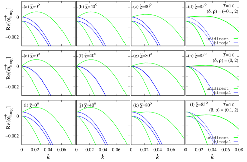
Figure 9: The dispersions of the average growth rate ${\rm Re}\,[\bar{\omega}^{\pm}_{\rm long}]$ of the longitudinal dune under the bimodal wind with $T=10$ for various slant angle $\tilde{\chi}$ in the wavy unstable regime, $(\delta,\rho)=(-0.1,2)$ (upper), $(0,2)$ (middle), and $(0.1,2)$ (lower). The dispersions under the unidirectional wind are also shown for comparison. The parameters are $h_{0}=5$, $q=1$, $D_{u}=1$, $T_{e}(h_{0})=1$, $(A,B,C)=(0.1,0.5,0.5)$ with $T_{e}^{\prime}(h_{0})=(T_{e}(h_{0})/h_{0})\delta$ and $D_{d}=D_{u}\rho$.

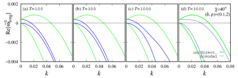
Figure 10: The dispersions of the average growth rate ${\rm Re}\,[\bar{\omega}^{\pm}_{\rm long}]$ of the longitudinal dune under the bimodal wind for various values of $T$ with the slant angle $\tilde{\chi}=40^{\circ}$ as $(\delta,\rho)=(0.1,2)$ along with those under the unidirectional wind for comparison. The parameters are $h_{0}=5$, $q=1$, $D_{u}=1$, $T_{e}(h_{0})=1$, $(A,B,C)=(0.1,0.5,0.5)$ with $T_{e}^{\prime}(h_{0})=(T_{e}(h_{0})/h_{0})\delta$ and $D_{d}=D_{u}\rho$.

The duration time $T$ dependence of the dispersion is shown in Fig. 10; the dispersion for the bimodal wind approaches toward those for the unidirectional wind for very large $T$ as is expected.

VI Simulations under bimodal winds of isolated straight transverse and longitudinal dunes with finite length

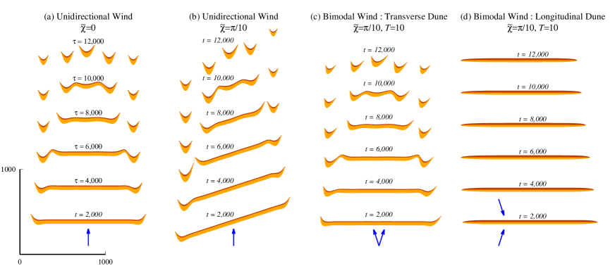
Figure 11: The time evolutions of the dune obtained by simulations of the crest line model for the unidirectional wind with $\tilde{\chi}=0$ (a) and $\pi/10$ (b), the transverse dune (c) and the longitudinal dune (d) under the bimodal wind dune with $\tilde{\chi}=\pi/10$ and $T=10$. The arrows show the directions of the wind for each case. The parameters are $(\delta,\rho)=(0,2)$, which is in the wavy unstable regime for the perturbation. The geometrical parameters for the cross section are $(A,B,C)=(0.1,0.8,0.2)$ for the dune under the unidirectional wind and the transverse dune, $(A,B,C)=(0.1,0.5,0.5)$ for the longitudinal dune. The initial state are given in the text. The advances of the dunes are represented by the vertical positions except for the case of the longitudinal dune, in which case the dune does not actually advance in the vertical direction.

We perform numerical simulations for the crest line model (8) and (9) for an isolated straight dune with finite length, and compare them with the results of linear analysis given above. The initial state is given by

$$h(y) =\left\{\begin{array}[]{ll}h_{0}(L_{y}/2+y)/L_{b}&\mbox{for $-L_{y}/2\leq y\leq-L_{y}/2+L_{b}$}\\ h_{0}&\mbox{for $-L_{y}/2+L_{b}<y<L_{y}/2-L_{b}$}\\ h_{0}\,(L_{y}/2-y)/L_{b}&\mbox{for $L_{y}/2-L_{b}\leq y\leq L_{y}/2$}\\ 0&\mbox{otherwise}\end{array}\right.,$$ (64)

$$x(y) =y\tan\chi$$ (65)

with the 1% of noise added to $h$. Here, $L_{y}=1500$, $L_{b}=L_{y}/20$, and $h_{0}=5$ in the units of Eq.(48). We take $D_{d}=2$, thus for the initial state, $(\delta,\rho)=(0,2)$, it is in the wavy unstable regime with $k_{\rm max}\approx{0.22\times 10^{-1}}$ and $\omega^{+}_{k_{\rm max}}\approx{0.69\times 10^{-3}}$ for $\chi=0$.

Since the model is defined in the way that the wind always blows in the $x$ direction, the crest line $\big{(}x(y),h(y)\big{)}$ needs to be rotated in the $x-y$ plane every time when the wind direction changes. The difficulty in this procedure is that the function $x(y)$, which represents the position of the crest line, may become multi-valued after the rotation, to which case the present model is not extended. To avoid this difficulty, we employ simplified transformations instead of the rotation, namely,

$$\Big{(}x(y),\;h(y)\Big{)}\quad\rightarrow\quad\Big{(}x(y)-2y\tan\chi,\;h(y)\Big{)},$$ (66)

for the bimodal wind in the case of transverse dune,

$$\Big{(}x(y),\;h(y)\Big{)}\quad\rightarrow\quad\Big{(}-x(-y)-2y\tan\chi,\;h(-y)\Big{)},$$ (67)

in the case of longitudinal dune every time when the wind direction changes. These are analogous to the ones used in the linear analysis and the difference between this simplified transformations and the rotations is small when $\chi$ and $x(y)-y\tan\chi$ are small.

Fig.11 shows the time evolutions of sand dune for $\tilde{\chi}=0$ (a) and $\pi/10$ (b) under the unidirectional wind, and those for the transverse (c) and the longitudinal (d) dunes under the bimodal wind with $T=10$ and $\tilde{\chi}=\pi/10$. The time evolution of the dune under the unidirectional wind with $\tilde{\chi}=\pi/10$ (b) and that of the transverse dune under the bimodal wind (c) are quite similar to that of the one under the unidirectional wind with $\tilde{\chi}=0$ (a); all of them show the instability with nearly the same wave number. On the other hand, in the case of the longitudinal dune with $\tilde{\chi}=\pi/10$ under the bimodal wind, the instability does not appear and the straight crest line is stable even though the parameters are in the region of the wavy unstable regime for the unidirectional wind. These results are completely consistent with those of the linear analysis given in Sec.V.

One may notice that the dune length decreases in time in our simulations while it has been observed that dunes often elongate in the average wind direction Tsoar et al. (2004). The reason for the shortening of the dune length in our simulations is that our simulations are performed under the condition of no influx, i.e. $f_{\rm in}=0$, thus the system lose sand grains at the ends of the dune, where the efficiency rate $T_{e}<1$ because $h<h_{c}$. It should be noted that, even with this setting, we observe the cases where the dune elongate toward the downwind direction if we use larger skew angle.

VII Concluding remarks

Advantages and disadvantages of the crest line model:

The crest line model used in the present study is one of the simplest model for the dune dynamics, where the dune configuration is described only by the position $x$ and the height $h$ of the crest as a function of $y$, assuming a similar triangle for the dune cross section along the wind direction. Its dynamics is determined by the sand transportations along the longitudinal and the lateral directions, which are characterized by a small number of phenomenological parameters and functions, i.e. $f_{\rm in}$, $q(h)$, $T_{e}(h)$, $D_{u}$, and $D_{d}$. Despite its simplicity, the model is capable to reproduce basic features of the dune dynamics.

Due to its simplicity, there are some obvious drawbacks. The model cannot describe the evolution of dunes of general forms, such as star dunes, that cannot be characterized by the geometrical parameters. The model in the original form is for a single dune, thus ignores the interaction between dunes. The parameters are largely phenomenological, thus it is not straightforward to derive them from elementary processes; the lateral sand fluxes, for example, are characterized simply by the diffusion constants $D_{u}$ and $D_{d}$, but the diffusion processes actually represent combined effects of biased random motion of sand grains due to saltation, reptation, creeping, avalanche, etc. These processes are excited by turbulent and helical flows over the dune, thus $D_{u}$ and $D_{d}$ may well depend on $q$ or some other parameters/variables although they are assumed to be constant in the present paper.

The advantages of the crest line model are also due to its simplicity; we can perform the stability analysis almost by hand even for the cases under the bimodal wind, and can analyze the results rather systematically to understand how the longitudinal dune becomes stable under the bimodal wind with large variation of the wind direction.

The present analysis show that the developed straight longitudinal dune with $\delta=0$, or $T_{e}^{\prime}=0$, is stable. However, it is often observed in the field that the longitudinal dunes especially without vegetation are undulating and are called seifPye and Tsoar (2009). We do not know yet how the vegetation effects may be incorporated in the crest line model, but our results suggest that the undulation in the longitudinal dune may arise during the dune developing process because the dispersions in the lower panel of Fig.9 for $(\delta,\rho)=(0.1,2)$ have an unstable part around $k=0$; The dune with $\delta>0$ is growing one because it is not yet saturated, i.e. $T_{e}^{\prime}>0$. These unstable modes can result in the undulation during the growth process if there are some effects that suppress the instability of the uniform mode with $k=0$, thus the maximum growth mode becomes at $k\neq 0$.

Parameter estimate:

Let us now estimate some of the parameter values in our model. Important ones are the critical dune height $h_{c}$ and the saturated sand flux $q_{c}$ over the crest of the critical height $h_{c}$. From the numerical results of fluid dynamics modellingWarren (2013); Momiji (2001), they might be estimated as

$$h_{c}\sim 5{\rm\,m},\qquad q_{c}\sim 5.9\times 10^{-6}{\rm\,m^{2}/s}.$$ (68)

This estimate for $q_{c}$ leads to the migration speed of dune $v$ of the crest height $h_{c}$ as

$$v={q_{c}\over h_{c}}\sim 38{\rm\,m/year}$$ (69)

in the case of perfect trapping without influx/outflux, i.e. $T_{e}=1$ and $f_{\rm in}=0$. This is actually consistent with the field observation data for the migration speed $v_{\rm obs}$ of the dunes with the height of 5 m (Fig.23.24 of Cooke et al. (1993)),

$$15{\rm\,m/year}\lesssim v_{\rm obs}\lesssim 50{\rm\,m/year}.$$ (70)

For the time unit of Eq.(48), the above estimates of Eq.(68) gives

$${h_{c}^{2}\over q_{c}}\sim 0.13{\rm\;year}.$$ (71)

Thus, our choice of $T=10$ for the duration of bimodal wind corresponds to 1.3 year, which is a little too longer as it should be 0.5 year, but we believe that the discrepancy is not significant, considering the accuracy of the above estimate. It should be also pointed out that most of our numerical results would barely change even if we use smaller value for $T$ because $T=10$ is already well in the small $T$ limit, and the approximations in Eqs.(53) and (55) are very good.

The spatial scale in the $y$ direction, or the lateral direction, is given by $h_{c}\sqrt{D_{u}/q_{c}}$ in Eq.(48). This contains a phenomenological parameter $D_{u}$, whose value should be a result of various processes under the influence of fluctuating wind averaged over the duration time, therefore, difficult to estimate from “microscopic processes”. However, the present stability analysis would give an estimate for $D_{u}$ as follows. For the transverse dune under the unidirectional wind, the dispersion curves in Fig.6 for $\tilde{\chi}=0^{\circ}$ and $(\delta,\rho)=(0,2)$, which corresponds to the well-developed dune, show the most unstable mode at around $k_{\rm max}\approx 0.025$, or in the length scale, it is $\lambda_{\rm max}\approx 250$ m. This actually coincides with the lateral size of the barchans with the height $h_{0}=5$ in Fig.11(a). If we know observation data for the barchan width $W_{\rm obs}$, then we can estimate the value of $D_{u}$ from the relation

$$W_{\rm obs}\approx\lambda_{\rm max}h_{c}\sqrt{D_{u}\over q_{c}}.$$ (72)

As a rough estimate, if we use $W_{\rm obs}\approx 250$ m for the dune with the height $h_{0}=5h_{c}\approx 25$ m, then the unit length in the $y$ direction is estimated as

$$h_{c}\sqrt{D_{u}\over q_{u}}\sim 1{\rm\,m},$$ (73)

which means that the length scale in the $y$ direction, i.e. the direction perpendicular to the wind, should be reduced by the factor 1/5 in Fig.11. This also gives

$$D_{u}\sim{q_{c}\over 25}\sim 0.24\times 10^{-6}{\rm\,m^{2}/s},$$ (74)

which turns out to be several orders of magnitude smaller than 4.0 $\rm m^{2}/s$, i.e. the value used for the diffusion constant by Schwämmle and HerrmannSchwämmle and Herrmann (2005), but it should be pointed out that $D_{u}$ in the crest line model is a phenomenological parameter, thus cannot be compared with the “microscopic” diffusion constant directly. With the estimate of Eq.(74), the relationship between $\chi$ and $\tilde{\chi}$ given by Eq.(49) becomes

$$\tan\chi\approx 5\tan\tilde{\chi},$$ (75)

which means $\chi>\tilde{\chi}$. Since most of our numerical results for $\tilde{\chi}=40^{\circ}$ are very close to the ones for $\tilde{\chi}=0^{\circ}$, we can conclude that the slant angle effect is very small for any value of $\chi<45^{\circ}$ except for the fact the spatial modulation along the crest line is elongated as Eq.(52).

Summary:

Using the crest line model, we examined the dynamical stability of the isolated straight sand dune under the unidirectional and the bimodal winds with the non-zero slant angle $\chi$. In the case of the unidirectional wind, we found that the linear stability for $\chi\neq 0$ remains the same with that for the wind with $\chi=0$. We extended the linear stability analysis to the case of bimodal winds and obtained the expressions for the growth rates for perturbation. Assuming the wind strengths and durations are the same for the both directions of the bimodal winds, we examined the two cases: the transverse dune, whose crest line is perpendicular to the average wind direction, and the longitudinal dune, whose crest line is parallel to the average wind. For the case of the unidirectional wind with $\chi\neq 0$ and for the case of the transverse dune, the dispersion curves of the growth rates virtually do not depend on the slant angle $\chi$ and are almost the same as those for the unidirectional wind for $\chi=0$ except for the case with very large slant angle, i.e. $\tilde{\chi}\gtrsim 80^{\circ}$, where the validity of the present model is not clear. On the other hand, in the case of the longitudinal dune, the dispersion curves of the growth rate change from those for the unidirectional wind so that the largest growth rate is always at $k=0$ even when the parameters are in the wavy unstable regime for the unidirectional wind case. This may be interpreted as a result of the fact that the growth of the perturbation with $k\neq 0$ is canceled by the alternating wind from opposite sides of the crest line even though it grows during each duration period of the bimodal wind. Mathematically, this cancellation is due to the existence of the decaying mode in the unidirectional case; The stabilization occurs because a major part of the growing mode is converted to the decaying mode whenever the wind direction switches.

The present study provides a theoretical framework for the stability analysis of sand dunes under the simple bimodal winds, and we demonstrated the stabilizing mechanism of a straight crest line for the longitudinal dune. This result qualitatively corresponds to the field observations and the computer simulations that the straight dunes tend to align to the average wind direction in the case of large seasonal variation of wind direction. It should be noted, however, that unvegetated linear dunes are often observed to have an undulating crest line, and straight dunes are usually vegetatedPye and Tsoar (1990); Parteli et al. (2009). It is also intriguing that almost straight longitudinal dune-like structures have been found in the images of TitanLorenz et al. (2006); Tokano (2008). Understanding detailed conditions for the undulation to appear/disappear in the longitudinal dunes is a theoretical problem in the next step.

References

- Bagnold (1941) R. Bagnold, The Physics of Blown Sand and Desert Dunes (Methuen, London, 1941).
- Pye and Tsoar (1990) K. Pye and H. Tsoar, Aeolian Sand and Sand Dunes (Unwin Hyman, London, 1990).
- Cooke et al. (1993) R. U. Cooke, A. Warren, and A. S. Goudie, Desert Geomorphology (UCL Press, London, 1993).
- Lancaster (1995) N. Lancaster, Geomorphology of Desert Dunes (Routledge, London, 1995).
- Warren (2013) A. Warren, Dunes: dynamics, morphology, history (Wiley & Sons, UK, 2013).
- Telfer et al. (2018) M. W. Telfer, E. J. R. Parteli, J. Radebaugh, R. A. Beyer, T. Bertrand, F. Forget, F. Nimmo, W. M. Grundy, J. M. Moore, S. A. Stern, J. Spencer, T. R. Lauer, A. M. Earle, R. P. Binzel, H. A. Weaver, C. B. Olkin, L. A. Young, K. Ennico, and K. Runyon, Science 360, 992 (2018).
- Andreotti et al. (2002a) B. Andreotti, P. Claudin, and S. Douady, Eur. Phys. J. B 28, 321 (2002a).
- Andreotti et al. (2002b) B. Andreotti, P. Claudin, and S. Douady, Eur. Phys. J. B 28, 341 (2002b).
- Kroy et al. (2002a) K. Kroy, G. Sauermann, and H. J. Herrmann, Phys. Rev. Lett. 88, 054301 (2002a).
- Kroy et al. (2002b) K. Kroy, G. Sauermann, and H. J. Herrmann, Phys. Rev. E 66, 031302 (2002b).
- Sauermann et al. (2001) G. Sauermann, K. Kroy, and H. J. Herrmann, Phys. Rev. E 64, 031305 (2001).
- Courrech du Pont et al. (2014) S. Courrech du Pont, C. Narteau, and X. Gao, Geology 42, 743 (2014).
- Rubin and Hunter (1987) D. M. Rubin and R. E. Hunter, Science 237, 276 (1987).
- Rubin and Ikeda (1990) D. M. Rubin and H. Ikeda, Sedimentology 37, 673 (1990).
- Taniguchi et al. (2012) K. Taniguchi, N. Endo, and H. Sekiguchi, Geomorphology 179, 286 (2012).
- Reffet et al. (2010) E. Reffet, S. Courrech du Pont, P. Hersen, and S. Douady, Geology 38, 491 (2010).
- Parteli et al. (2009) E. Parteli, O. Durán, H. Tsoar, V. Schwämmle, and H. Herrmann, PNAS 106, 22085 (2009).
- Parteli and Herrmann (2007) E. J. R. Parteli and H. J. Herrmann, Phys. Rev. Lett. 98, 198001 (2007).
- Werner and Kocurek (1997) B. Werner and G. Kocurek, Geology 25, 771 (1997).
- Gadal et al. (2019) C. Gadal, C. Narteau, S. Courrech du Pont, O. Rozier, and P. Claudin, Journal of Fluid Mechanics 862, 490–516 (2019).
- Werner (1995) B. T. Werner, Geology 23, 1107 (1995).
- Nishimori and Ouchi (1993) H. Nishimori and N. Ouchi, Phys. Rev. Lett. 71, 197 (1993).
- Nishimori et al. (1998) H. Nishimori, M. Yamasaki, and K. H. Andersen, International Journal of Modern Physics B 12, 257 (1998).
- Guignier et al. (2013) L. Guignier, H. Niiya, H. Nishimori, D. Lague, and A. Valance, Phys. Rev. E 87, 052206 (2013).
- Niiya et al. (2010) H. Niiya, A. Awazu, and H. Nishimori, Journal of the Physical Society of Japan 79, 063002 (2010).
- Niiya et al. (2012) H. Niiya, A. Awazu, and H. Nishimori, Phys. Rev. Lett. 108, 158001 (2012).
- Momiji and Warren (2000) H. Momiji and A. Warren, Earth Surface Processes and Landforms 25, 1069 (2000).
- Note (1) Since , , and have the same dimension of unit, there are actually three possible ways to interpret the numerical values depending on the choice of two quantities out of the three to be assigned to the same unit. We prefer and to be in the same unit because the geometrical parameters , , and do not depend on the constants of Eq.(47). In this choice, however, the slant angle depends on as in Eq.(49). .
- Note (2) In the following, numerical values for the slant angle are always given by defined in Eq.(49), but the slant angle in the mathematical expressions should be the original slant angle . .
- Note (3) It is interesting to see that the average growth rate for the bimodal wind can be larger than the growth rate for the unidirectional wind. This means that the largest absolute value of the eigenvalue of the evolution matrix is larger than the product of the largest absolute values of the eigenvalue of each factor matrix in Eq.(41).
- Tsoar et al. (2004) H. Tsoar, D. G. Blumberg, and Y. Stoler, Geomorphology 57, 293 (2004).
- Pye and Tsoar (2009) K. Pye and H. Tsoar, in Aeolian Sand and Sand Dunes (Springer, Berlin, Heidelberg, 2009) Chap. 6, pp. 175–253.
- Momiji (2001) H. Momiji, Mathematical modelling of the dynamics and morphology of aeolian dunes and dune fields, Ph.D. thesis, University College London (2001).
- Note (4) From the numerical estimates of the trapping efficiency (Fig.3.3 at p.50 of Warren (2013)) and the friction velocity (Fig.4.5 at p.88 of Momiji (2001)), we obtain the estimates and 0.5 m/s. For this value of the friction velocity, the mass flux at the crest can be estimated as kg/m s from Fig.1.8 in p.28 of Warren (2013) . The volume flux is given by with the mass density of sand .
- Schwämmle and Herrmann (2005) V. Schwämmle and H. Herrmann, Eur. Phys. J. E 16, 57 (2005).
- Lorenz et al. (2006) R. D. Lorenz, S. Wall, J. Radebaugh, G. Boubin, E. Reffet, M. Janssen, E. Stofan, R. Lopes, R. Kirk, C. Elachi, J. Lunine, K. Mitchell, F. Paganelli, L. Soderblom, C. Wood, L. Wye, H. Zebker, Y. Anderson, S. Ostro, M. Allison, R. Boehmer, P. Callahan, P. Encrenaz, G. G. Ori, G. Francescetti, Y. Gim, G. Hamilton, S. Hensley, W. Johnson, K. Kelleher, D. Muhleman, G. Picardi, F. Posa, L. Roth, R. Seu, S. Shaffer, B. Stiles, S. Vetrella, E. Flamini, and R. West, Science 312, 724 (2006).
- Tokano (2008) T. Tokano, Icarus 194, 243 (2008).