Pareto models for risk management

by

Arthur Charpentier
Université du Québec à Montréal (UQAM)
201, avenue du Président-Kennedy,
Montréal (Québec), Canada H2X 3Y7
arthur.charpentier@uqam.ca

and

Emmanuel Flachaire
Aix-Marseille Université
AMSE, CNRS and EHESS,
5 bd Maurice Bourdet,
13001, Marseille, France,
emmanuel.flachaire@univ-amu.fr

December 2019

Abstract

The Pareto model is very popular in risk management, since simple analytical formulas can be derived for financial downside risk measures (Value-at-Risk, Expected Shortfall) or reinsurance premiums and related quantities (Large Claim Index, Return Period). Nevertheless, in practice, distributions are (strictly) Pareto only in the tails, above (possible very) large threshold. Therefore, it could be interesting to take into account second order behavior to provide a better fit. In this article, we present how to go from a strict Pareto model to Pareto-type distributions. We discuss inference, and derive formulas for various measures and indices, and finally provide applications on insurance losses and financial risks.

JEL: C13; C18; C46; G22; G32

Keywords: EPD; Expected Shortfall; Financial Risks; GPD; Hill; Pareto; Quantile; Rare events; Regular Variation; Reinsurance; Second Order; Value-at-Risk;

1 Introduction

The Gaussian distribution is one of the most popular distribution used initially to model observation errors. It can be used to model individual measurements that are (somehow) centered, such as the height, or the weight of individuals. But not all data exhibit such a property, where the distribution has a peak around a typical value (the median or the mean), such as the distribution of the population among cities, or the distribution of wealth among individuals. Those distribution are known to be right-skewed, where most observations are bulked with small values, a small proportion can reach much higher values than the median (or the mean), leading to long tail on the right of the distribution. For instance, Pareto introduced the following model for the distribution of income: let $p(x)dx$ denote the proportion of individuals with income between $x$ and $x+dx$; if the histogram is a straight line on the log-log scales, then $\log p(x)=a-b\log(x)$ (since the slope is clearly always negative), or equivalently, $p(x)=cx^{-b}$. Such distributions are said to have a power law, or a Pareto distribution since it was introduced by the economist Vilfredo Pareto (see CharpentierFlachaire for applications to model income distributions). The constant $b$ might be called the exponent of the power law (especially in the context of networks or in physical applications), but in economic application, the exponent will be the one of the survival distribution ${S(x)=\int_{x}^{\infty}p(y)dy}$, which is also a power function, with index $1+b$.

The Gaussian distribution is a natural candidate when focusing on the center of the distribution, on average values, because of the central limit theorem: the Gaussian distribution is stable by summing, and averaging. If $\{X_{1},\cdots,X_{n}\}$ are independent Gaussian variables, so is $X_{1}+\cdots+X_{n}$ (and any linear transformation). As mentioned in Jenssen:06 and Gabaix, the power distribution satisfies similar interesting properties: if $X_{1}$ is a power distribution with exponent $b_{1}$, independent of $X_{2}$, another power distribution with exponent $b_{2}$, with $b_{2}\geq b_{1}$, then $X_{1}+X_{2}$, $X_{1}\cdot X_{2}$, or $\max\{X_{1},X_{2}\}$ are also power distributed, with exponent $b_{1}$. And those properties of invariance and stability are essential in stochastic modeling. As mentioned in Schumpeter, in an obituary article about Vilfredo Pareto, “few if any economists seem to have realized the possibilities that such invariants hold for the future of our science. In particular, nobody seems to have realized that the hunt for, and the interpretation of, invariants of this type might lay the foundations for an entirely novel type of theory”. If several applications can be found on proportional (random) growth theory (as discussed in Gabaix, with connections to recursive equations), or on matching and networks, an important application of this Pareto model is risk management.

Insurers and actuaries have used Pareto distribution to model large losses since Hagstroem:25 (Hagstroem:25, Hagstroem:60). BaHa:74 suggested to use such a distribution in a life-insurance context (to model the remaining lifetimes for very old people), but the Pareto distribution has mainly been used to model (large) insurance losses since reinsurance premiums have simple and analytical expression, as in Vajda:1951, even for more complex treaties than standard stop-loss or excess-of-loss treaties as in Kremer1984. BeirlantTeugels1992, McNeil:1997 (discussed in Resnick:1997) and EKM discussed more applications in insurance, with connections to extreme value theory.

The Value-at-Risk has been the finance benchmark risk measure for the past 20 years. Estimating a quantile for small probabilities, such as the 1%-quantile of the profit and loss distribution for the next 10 days. Historically, practitioners used a standard Gaussian model, and then multiply by a factor of $3$ (as explained in Klup:04, this factor 3 is supposed to account for certain observed effects, also due to the model risk; it is based on backtesting procedures and can be increased by the regulatory authorities, if the backtesting proves the factor 3 to be insufficient). A less ad hoc strategy is to use a distribution that fits better tails of profit and loss distribution, such as the Pareto one.

Nevertheless, if the Pareto distribution remains extremely popular because several quantities can easily be derived (risk measures or insurance premium), in practice, distributions are only Pareto in very high tails (say above the 99.9% quantile). So it becomes necessary to take into account second order approximation, to provide a better fit. Thus, we will see in this article how to derive risk measures and insurance premiums when distribution are Pareto-type above a (high) threshold $u$.

In Section 2, we will define the two popular Pareto models, the strict Pareto distribution and the Generalized Pareto distribution (GPD), emphasizing differences between the two. A natural extension will be related to the concept of Pareto-type distribution, using regular variation function. In Section 3, we will get back on the concepts of regular variation, and present the Extended Pareto distribution (EPD), introduced in BeJoSe:09. The inference of Pareto models will be discussed in Section 4, with a discussion about the use of Hill estimator, still very popular in risk management, and Maximum Likelihood estimation. In Section 5 we will define classical measures and indices, and discuss expression and properties when underlying distribution are either strict Pareto, or Pareto-type, with high quantiles ($Q$), expected shortfall (ES), and large claim or top share indices (TS). And as Pareto models are usually assumed above a high threshold $u$ we will see, at the end of that section, how analytical expressions of those measures can be derived when Pareto-type distributions are considered only above threshold $u$ (and define $Q_{u}$, $\text{ES}_{u}$, etc). Finally, applications on real data will be considered, with insurance and reinsurance pricing in Section 6 and log-returns and classical financial risk measures in Section 7.

2 Strict Pareto models

Pareto models are obtained when the loss distribution $\mathbb{P}[X>x]$ exhibits a power decay $x^{-\alpha}$. From a mathematical perspective, such a power function is interesting because it is the general solution of Cauchy’s functional equation (its multiplicative version), $h(x\cdot y)=h(x)\cdot h(y)$, $\forall x,y$. A probabilistic interpretation is the stability of the conditional distribution $X$ given $X>u$ for any threshold $u$: the conditional distribution still exhibits a power decay, with the same index. But if we try to formalize more, two distributions will be obtained: a Pareto I distribution will be obtained when modelling the distribution of relative excesses $X/u$ given $X>u$ - see Equation (1) - while the GPD (Generalized Pareto Distribution) will be obtained when modelling the distribution of absolute excesses $X-u$ given $X>u$ - see Equation (6).

2.1 Pareto I distribution

A Pareto Type I distribution, bounded from below by $u>0$, with tail parameter $\alpha$, has probability density function and cumulative density function (CDF) equal to

$$f(x)=\frac{\alpha u^{\alpha}}{x^{\alpha+1}}\qquad\text{and}\qquad F(x)=1-\left(\frac{x}{u}\right)^{-\alpha},\qquad\text{for }x\geq u$$ (1)

If a random variable $X$ has distribution (1), we will write $X\sim{\cal P}_{1}(u,\alpha)$. This distribution has an attractive property: the average above a threshold is proportional to the threshold, and it does not depend on the scale parameter $u$,

$$\mathbb{E}(X|X>u^{\prime})=\frac{\alpha u^{\prime}}{\alpha-1},\qquad\alpha>1$$ (2)

where $u^{\prime}\geq u$. Such a function is related to the mean excess function – or expected remaining lifetime at age $u^{\prime}$ when $X$ denotes the (random) life length – defined as

$$e(u^{\prime})=\mathbb{E}(X-u^{\prime}|X>u^{\prime}).$$ (3)

In the case of a Pareto distribution, it is also a linear function

$$e(u^{\prime})=\frac{u^{\prime}}{\alpha-1},\qquad\alpha>1$$ (4)

Remark 1

In several textbooks and articles, Pareto models are defined with tail index $\xi=1/\alpha$, so that the survival function is proportional to the power function $x^{-1/\xi}$, instead of $x^{-\alpha}$. In that case, we have the confusing expressions

$$\mathbb{E}(X|X>u^{\prime})=\frac{u^{\prime}}{1-\xi}\quad\text{ and }\quad e(u^{\prime})=\frac{\xi u^{\prime}}{1-\xi},\qquad\xi<1.$$ (5)

2.2 Generalized Pareto distribution

A Generalized Pareto Distribution (GPD), bounded from below by $u\geq 0$, with scale parameter $\sigma$ and tail parameter $\alpha$, has cumulative density function (CDF)

$$F(x)=1-\left[1+\left(\frac{x-u}{\sigma}\right)\right]^{-\alpha}\qquad\text{for }x\geq u$$ (6)

where $\sigma>0$ and $\alpha\in(0,\infty]$. If a random variable $X$ has distribution (6), we will write $X\sim{\cal GPD}(u,\sigma,\alpha)$. The ${\cal GPD}(0,\sigma,\alpha)$ distribution is also called “Lomax” in the literature Lomax:54. The GPD is “general” in the sense that Pareto I distribution is a special case, when $\sigma=u$:

$${\cal{GPD}}(u,u,\alpha)={\cal{P}}_{1}(u,\alpha)$$ (7)

Scollnik07 suggested an alternative expression, instead of (6),

$$F(x)=1-\left[\frac{u+\lambda}{x+\lambda}\right]^{\alpha}\qquad\text{for }x\geq u$$ (8)

where $\lambda=\sigma-u$. Note that this function is used in GAMLSS to introduce a regression type model, where both $\lambda$ and $\alpha$ will be the exponential of linear combinations of some covariates, as in the gamlss package, in R.

Remark 2

In several textbooks and articles, not only the Generalized Pareto has tail index $\xi=1/\alpha$, but $\xi$ appears also in the fraction term

$$F(x)=1-\left[1+\xi\left(\frac{x-u}{\sigma}\right)\right]^{-1/\xi}\qquad\text{for }x\geq u,$$ (9)

which could be seen as a simple alternative expression of the shape parameter $\sigma$. This expression is interesting since the limit when $\xi$ tends to $0$ can easily be defined, as well as the case where $\xi<0$, which could be interesting in extreme value theory.

The average above a higher threshold, $u^{\prime}\geq u$, depends now on all parameters of the distribution,

$$\mathbb{E}(X|X>u^{\prime})=\frac{\sigma-u}{\alpha-1}+\frac{\alpha}{\alpha-1}u^{\prime},\$$ (10)

The linearity of this function (as well as the mean excess function) characterizes the GPD class (see GuessProschan:88 and GhoshResnick:10). A sketch of the proof is that we want

$$e(u^{\prime})=\mathbb{E}(X|X>u^{\prime})=\frac{1}{\overline{F}(u^{\prime})}\int_{u^{\prime}}^{\infty}xdF(x)=A+Bu^{\prime},$$ (11)

or, when differentiating with respect to $u^{\prime}$, we obtain

$$B\overline{F}(u^{\prime})du^{\prime}=s-\big{[}A+(B-1)u^{\prime}\big{]}d\overline{F}(u^{\prime}),$$ (12)

thus, up to some change of parameters

$$\frac{d\overline{F}}{\overline{F}}=-\alpha\frac{du}{u+c}\quad\text{ with }\quad\alpha=\frac{B}{B-1}$$ (13)

which is a GPD distribution, with tail index $\alpha$.

One of the most important result in the extreme value theory states that, for most heavy-tailed distributions, the conditional excess distribution function, above a threshold $u$, converges towards a GPD distribution as $u$ goes to infinity (Pick:75, BaHa:74), for some parameters $\alpha$ and $\sigma$,

$${F}_{u}(x)\longrightarrow\text{ GPD (or Pareto II) \quad as }u\rightarrow+\infty$$ (14)

where ${F}_{u}(x)=P(X-u\leq x|X>u)$. This result is known as the Pickands-Balkema-de Haan theorem, also called the second theorem in extreme value theory (as discussed in footnote 2, footnote 2). It provides strong theoretical support for modelling the upper tail of heavy-tailed distributions with GPD, also known as the Pareto Type II distribution. In a very general setting, it means that there are $\alpha$ and $\sigma$ such that $F_{u}$ can be approximated by the CDF of a $\mathcal{GPD}(u,\sigma,\alpha)$, see EKM (EKM, Theorem 3.4.13, p.165).

2.3 Threshold selection

Whether to use a Pareto I or GPD model to fit the upper tail is related to the choice of the threshold. From (1) and (6), we have seen that Pareto I is a special case of GPD, when $\sigma=u$. They differ by an affine transformation when $\sigma\not=u$. A key property of Pareto distributions is that, if a distribution is Pareto for a fixed threshold $u$, it is also Pareto with the same tail parameter $\alpha$ for a higher threshold $u^{\prime}\geq u$. For GPD, we have

$$\overline{F}_{u}={\cal{GPD}}(u,\sigma,\alpha)\quad\Rightarrow\quad\overline{F}_{u^{\prime}}={\cal{GPD}}(u^{\prime},\sigma+u^{\prime}-u,\alpha).$$ (15)

where $\overline{F}_{u}$ is the survival excess function above $u$. Thus, Pareto I and GPD are the same for all $u^{\prime}\geq u$, if $\sigma=u$. Otherwise, we have $\sigma+u^{\prime}-u\approx u^{\prime}$ for very large values of $u^{\prime}$ only. It follows that a GPD above a threshold will behave approximately as a Pareto I above a higher threshold, much higher as $\sigma$ differs from $u$. This point will be discussed further in section 5.5.

3 Pareto-type models

Since our interesting in risk management is usually motivated by the description of so-called downside risks, or (important) losses, as described in Roy:1952. Thus, we do not need that have a (strict) Pareto distribution for all $x$’s, in $\mathbb{P}[X>x]$, but possibly only when $x$’s are large enough. In this section, we will introduce some regular variation concepts, used to model that asymptotic property, and exhibit a distribution that is not strictly Pareto, by introducing a second order effect: the Extended Pareto Distribution.

3.1 First- and second-order regular variation

The tail index $\alpha$ is related to the max-domain of attraction of the underlying distribution, while parameter $\sigma$ is simply a scaling parameter. The shape of the conditional excess cumulative distribution function is a power function (the Pareto distribution) if the threshold is large enough. Tails are then said to be Pareto-type, and can be described using so called regularly varying functions (see BiGoTe:87).

First and second order regular variation were originally used in extreme value theory, to study respectively the tail behavior of a distribution and the speed of convergence of the extreme value condition (see BiGoTe:87, HaSt:96, PeQi:04, or section 2 in HaFe:06 for a complete survey). A function $H$ is said to be regularly varying (at infinity) with index $\gamma\in\mathbb{R}$ if

$$\lim_{t\rightarrow\infty}\frac{H(tx)}{H(t)}=x^{\gamma}~{}\text{ or }~{}\lim_{t\rightarrow\infty}x^{-\gamma}\frac{H(tx)}{H(t)}=1.$$ (16)

A function regularly varying with index $\gamma=0$ is said to be slowly varying. Observe that any regularly varying function of index $-\gamma$ can be written $H(x)=x^{-\gamma}\ell(x)$ where $\ell$ is some slowly varying function.

Consider a random variable $X$, its distribution is regularly-varying with index $-\gamma$ if, up-to some affine transformation, its survival function is regularly varying. Hence,

$$\lim_{t\rightarrow\infty}x^{-\gamma}\frac{\overline{F}(tx)}{\overline{F}(t)}=1$$ (17)

or

$$\overline{F}(x)=x^{-\gamma}\ell(x),$$ (18)

where $\overline{F}(x)=1-F(x)$. A regularly varying survival function is then a function that behaves like a power law function near infinity. Distributions with survival function as defined in (18) are called Pareto-type distributions. It means that the survival function tends to zero at polynomial (or power) speed as $x\rightarrow\infty$, that is, as $x^{-\gamma}$. For instance, a Pareto I distribution, with survival function $\overline{F}(x)=x^{-\alpha}u^{\alpha}$, is regularly varying with index $-\alpha$, and the associated slowly varying function is the constant $u^{\alpha}$. And a GPD or Pareto II distribution, with survival function $\overline{F}(x)=\left(1+\sigma^{-1}{x}\right)^{-\alpha}$, is regularly varying with index $-\alpha$, for some slowly varying function. But in a general setting, if the distribution is not strictly Pareto, $\ell$ will not be constant, and it will impact the speed of convergence.

In HaSt:96, a concept of second-order regular variation function is introduced, that can be used to derive a probabilistic property using the quantile function, as in BeGoSeTe:04. Following BeJoSe:09, we will consider distributions such that an extended version of equation (17) is satisfied,

$$\lim_{t\rightarrow\infty}x^{-\gamma}\frac{\overline{F}(tx)}{\overline{F}(t)}=1+\frac{x^{\rho}-1}{\rho},\text{ for some }\rho\leq 0,$$ (19)

that we can write, up to some affine transformation,

$$\overline{F}(x)=cx^{-\gamma}[1-x^{\rho}\ell(x)],$$ (20)

for some slowly varying function $\ell$ and some second-order tail coefficient $\rho\leq 0$. The corresponding class of Pareto-type distributions defined in (20) is often named the Hall class of distributions, referring to Hall:82. It includes the Singh-Maddala (Burr), Student, Fréchet and Cauchy distributions. A mixture of two strict Pareto-I distributions will also belong to this class.

Since $\rho\leq 0$, $x\mapsto 1-x^{\rho}\ell(x)$ is slowly varying, and therefore, a distribution $\overline{F}$ that satisfies (20) also satisfies (18). More specifically, in (20), the parameter $\rho$ captures the rate of convergence of the survival function to a strict Pareto distribution. Smaller is $\rho$, faster the upper tail behaves like a Pareto, as $x$ increases. Overall, we can see that

• $\gamma$ is the first-order of the regular variation, it measures the tail parameter of the Pareto distribution,

• $\rho$ is the second-order of the regular variation, it measures how much the upper tail deviates from a strictly Pareto distribution.

In the following, we will write RV$(-\gamma,\rho)$. There are connections between tail properties of the survival function $\overline{F}$ and the density $f$ (see also Karamata theory for first order regular variation). More specifically, if $\overline{F}$ is RV$(-\gamma,\rho)$, with $\gamma>1$, then $f$ is RV$(-\gamma-1,\rho)$.

For instance, consider a Singh-Maddala (Burr) distribution, with survival distribution $\overline{F}(x)=[1+x^{a}]^{-q}$, then a second order expansion yields

$$\overline{F}(x)=x^{-aq}[1-qx^{-a}+o(x^{-a})]~{}\text{as}~{}x\rightarrow\infty$$ (21)

which is regularly varying of order $-aq$ and with second order regular variation $-a$, that is RV$(-aq,-a)$.

3.2 Extended Pareto distribution

BeJoSe:09 show that Equation (20) can be approximated by

$$\overline{F}(x)=\left[x\left(1+\delta-\delta x^{\tau}\right)\right]^{-\alpha}\qquad\text{for }x\geq 1$$ (22)

where $\tau\leq 0$ and $\delta>\max(-1,1/\tau)$. The main feature of this function is that it captures the second-order regular variation of the Hall class of distributions, that is, deviation to a strictly Pareto tail, as defined in Hall:82,

$$\overline{F}(x)=ax^{-\alpha}\left[1+bx^{-\beta}+o(x^{-\beta})\right]$$ (23)

or, using Taylor’s expansion,

$$\overline{F}(x)=ax^{-\alpha}\left[1+b_{1}x^{-\alpha}+\cdots+b_{k}x^{-k\alpha}+o(x^{-k\alpha})\right]$$ (24)

with general notations. For more details, see also AlBeTe:17 (AlBeTe:17, section 4.2.1).

From (22), we can define the Extended Pareto Distribution (EPD), proposed by BeJoSe:09, as follows:

$$F(x)=1-\left[\frac{x}{u}\left(1+\delta-\delta\left(\frac{x}{u}\right)^{\tau}\right)\right]^{-\alpha}\qquad\text{for }x\geq u$$ (25)

where $\tau\leq 0$ and $\delta>\max(-1,1/\tau)$. If a random variable $X$ has (25) as its CDF, we will write $X\sim{\cal EPD}(u,\delta,\tau,\alpha)$.

Pareto I is a special case when $\delta=0$ and GPD is a special case when $\tau=-1$:

$${\cal EPD}(u,0,\tau,\alpha) =\quad{\cal P}_{1}(u,\alpha)$$ (26)

$${\cal EPD}(u,\delta,-1,\alpha) =\quad{\cal GPD}(1,u/(1+\delta),\alpha)$$ (27)

The mean over a threshold for the EPD distribution has no closed form expression. Numerical methods can be used to calculate it. Since $u^{\prime}\geq u>0$, $X$ given $X>u^{\prime}$ is a positive random variable and

$$\mathbb{E}[X|X>u^{\prime}]=\int_{0}^{\infty}\overline{F}_{u^{\prime}}(x)dx$$ (28)

where $\overline{F}_{u^{\prime}}(x)=\mathbb{P}[X>x|X>u^{\prime}]$ for $x>u$, i.e.

$$\overline{F}_{u^{\prime}}(x)=\frac{\overline{F}(x)}{\overline{F}(u^{\prime})}\quad\text{ where }\quad\overline{F}\text{ is the s.d.f. of }X$$ (29)

Thus

$$\mathbb{E}[X|X>u^{\prime}]=u^{\prime}+\frac{1}{\overline{F}(u^{\prime})}\int_{u^{\prime}}^{\infty}\overline{F}(x)dx$$ (30)

The integral in Equation (30) can be computed numerically. Since numerical integration over a finite segment could be easier, we can make a change of variable ($1/x$) to obtain an integral over a finite interval:

$$E_{u^{\prime}}=\int_{u^{\prime}}^{\infty}\overline{F}(x)dx=\int_{0}^{1/u^{\prime}}\frac{1}{x^{2}}\,\overline{F}\left(\frac{1}{x}\right)dx$$ (31)

The Extended Pareto distribution has a stable tail property: if a distribution is EPD for a fixed threshold $u$, it is also EPD for a higher threshold $u^{\prime}\geq u$, with the same tail parameter $\alpha$. Indeed, deriving a truncated EPD distribution, we find

$$\overline{F}_{u}={\cal{EPD}}(u,\delta,\tau,\alpha)\quad\Rightarrow\quad\overline{F}_{u^{\prime}}={\cal{EPD}}(u^{\prime},\delta^{\prime},\tau,\alpha).$$ (32)

where $\delta^{\prime}=\delta(u^{\prime}/u)^{\tau}/[1+\delta-\delta(u^{\prime}/u)^{\tau}]$. A plot of estimates of the tail index $\alpha$ for several thresholds would then be useful. If the distribution is Extended Pareto, a stable horizontal straight line should be plotted. This plot is similar to Hill plot for Hill estimates of $\alpha$ from Pareto I distribution. It is expected to be more stable if the distribution is not strictly Pareto. Indeed, EKM (EKM, p.194) and Resn:07 (Resn:07, p.87) illustrate that the Hill estimator can perform very poorly if the slowly varying function is not constant in (18). It can lead to very volatile Hill plots, also known as Hill horror plots. This will be discussed in section 4.1.

4 Inference based on Pareto type distributions

In this section, we briefly recall two general techniques used to estimate the tail index, and additional parameters: Hill estimator and maximum likelihood techniques. For further details, see EKM, HaFe:06 or BeGoSeTe:04, and references therein.

4.1 Hill’s Estimator

In the case where the distribution above a threshold $u$ is supposed to be $\mathcal{P}(u,\alpha)$, Hill’s estimator of $\alpha$ is

$$\widehat{\alpha}_{u}=\left(\frac{1}{n_{u}}\sum_{i=1}^{n_{u}}\log(x_{n+1-i:n})-\log(u)\right)^{-1}$$ (33)

This estimator is the maximum likelihood estimator of $\alpha$.

From Theorem 6.4.6 in EKM and section 4.2 in BeGoSeTe:04, if we assume that the distribution of $X$ is Pareto-type, with index $\alpha$, $\overline{F}(x)=x^{-\alpha}\ell(x)$, if $u\rightarrow\infty$, $n\rightarrow\infty$ and $n_{u}/n\rightarrow 0$, then $\widehat{\alpha}_{u}$ is a (strongly) consistent estimator of $\alpha$ when observations are i.i.d., and further, under some (standard) technical assumptions,

$$\sqrt{n_{u}}\big{(}\widehat{\alpha}_{u}-\alpha\big{)}\overset{\mathcal{L}}{\rightarrow}\mathcal{N}(0,\alpha^{2}).$$ (34)

This expression can be used to derive confidence interval for $\alpha$, but also any index mentioned in the previous section (quantile, expected shortfall, top shares, etc) using the $\Delta$-method. For instance

$$\frac{\sqrt{n_{u}}Q(1-p)}{\sqrt{1+(\log[n_{u}/n]-\log[p])^{2}}}\big{(}\widehat{Q}_{u}(1-p)-Q(1-p)\big{)}\overset{\mathcal{L}}{\rightarrow}\mathcal{N}(0,\alpha^{-2}),$$ (35)

as shown in Section 4.6. of BeGoSeTe:04.

Nevertheless, as discussed in EKM and BeGoSeTe:04, this asymptotic normality is obtained under some appropriate choice of $u$ (as a function of $n$) and $\ell$ : $u$ should tend to infinity sufficiently slowly, otherwise, $\widehat{\alpha}_{u}$ could be a biased estimator, even asymptotically. More specifically, in section 3.1, we introduced second order regular variation: in Equation (20), assume that $\ell(x)=-1$, so that

$$\overline{F}(x)=cx^{-\alpha}[1+x^{\rho}]$$ (36)

From Theorem 6.4.9 in EKM, if $n_{u}=o(n^{(2\rho)/(2\rho+\alpha)})$, then the asymptotic convergence of Equation (35) is valid. But if $n^{-(2\rho)/(2\rho+\alpha)}n_{u}$ tends to $\lambda$ as $n\rightarrow\infty$, then

$$\sqrt{n_{u}}\big{(}\widehat{\alpha}_{u}-\alpha\big{)}\overset{\mathcal{L}}{\rightarrow}\mathcal{N}\left(\frac{\alpha^{3}\lambda}{\rho-\alpha},\alpha^{2}\right),$$ (37)

has an asymptotic bias. Such a property makes Hill estimator dangerous to use for Pareto-type distributions.

4.2 Maximum Likelihood Estimator

For the GPD, a popular is to use the maximum likelihood estimator. When threshold $u$ is given, the idea is to fit a $\mathcal{GPD}(0,\sigma,\alpha)$ distribution on the sample $\{y_{1},\cdots,y_{n_{u}}\}=\{x_{n+1-n_{u}:n}-u,\cdots,x_{n:n}-u\}$. The density being

$$f(y;\sigma,\alpha)=\frac{\alpha}{\sigma}\left(1+\frac{y}{\sigma}\right)^{-\alpha-1}$$ (38)

the log-likelihood is here

$$\log\mathcal{L}(\sigma,\alpha;\boldsymbol{y})=-n\log\frac{\alpha}{\sigma}-(\alpha+1)\sum_{i=1}^{n_{u}}\left(1+\frac{y_{i}}{\sigma}\right).$$ (39)

As expected, the maximum likelihood estimator of $(\sigma,\alpha)$ is asymptotically Gaussian, as shown in Section 6.5 of EKM (with a different parameterization of the GPD). In the case of the Extended Pareto distribution, there might be numerical complications, but [Beirlant, Joossens, and SegersBeirlant et al.2009] provided theoretical properties, and ReIns provided R codes, used in AlBeTe:17.

Note that since $\alpha$ is usually seen as the most important parameter (and $\sigma$ is more a nuisance parameter) it can be interesting to use profile likelihood techniques to derive some confidence interval, as discussed in Section 4.5.2 in davison:2004. Consider some Pareto type model, with parameter $(\alpha,\boldsymbol{\theta})$. Let

$$(\widehat{\alpha},\widehat{\boldsymbol{\theta}})=\underset{\alpha,\boldsymbol{\theta}}{\text{argmax}}\left\{\log\mathcal{L}(\alpha,\boldsymbol{\theta})\right\}$$ (40)

denote the maximum likelihood estimator. From the likelihood ratio test, under technical assumptions,

$$2\big{(}\log\mathcal{L}(\widehat{\alpha},\widehat{\boldsymbol{\theta}})-\log\mathcal{L}(\alpha,\boldsymbol{\theta})\big{)} \rightarrow\chi^{2}\big{(}\text{dim}(\alpha,\boldsymbol{\theta})\big{)}$$

where $I_{n}(\alpha,\boldsymbol{\theta})$ is Fisher information. The idea of the profile likelihood estimator is to define, given $\alpha$

$$\widehat{\boldsymbol{\theta}}_{\alpha}=\underset{\boldsymbol{\theta}}{\text{argmax}}\left\{\log\mathcal{L}(\alpha,\boldsymbol{\theta})\right\}$$ (41)

and then

$$\widehat{\alpha}_{p}=\underset{\alpha}{\text{argmax}}\left\{\log\mathcal{L}(\alpha,\boldsymbol{\theta}_{\alpha})\right\}$$ (42)

Then

$$2\big{(}\log\mathcal{L}(\widehat{\alpha}_{p},\widehat{\boldsymbol{\theta}}_{\widehat{\alpha}_{p}})-\log\mathcal{L}(\alpha,\boldsymbol{\theta})\big{)} \rightarrow\chi^{2}\big{(}1)\big{)}.$$

Thus, if $\log\mathcal{L}_{p}(\alpha)$ denotes the profile likelihood, defined as $\log\mathcal{L}_{p}(\alpha)=\log\mathcal{L}(\alpha,\widehat{\boldsymbol{\theta}}_{\alpha})$, then a $95\%$ confidence interval can be obtained,

$$\big{\{}\alpha:\log\mathcal{L}_{p}(\alpha)\geq\log\mathcal{L}_{p}(\widehat{\alpha}_{p})-\frac{1}{2}q_{\chi^{2}(1)}(95\%)\big{\}}$$ (43)

where $q_{\chi^{2}(1)}(95\%)$ is the $95\%$ quantile of the $\chi^{2}(1)$ distribution.

4.3 Application on Simulated Data

In this section, three distributions where simulated: a strict Pareto on Figure 1 with tail index $\alpha=1.5$, a Generalized Pareto on Figure 2 with tail index $\alpha=1.5$, and an Extented Pareto on Figure 3 with tail index $\alpha=1.5$. Each time, on the left, the Hill plot is plotted, i.e. the plot $u\mapsto\widehat{\alpha}_{u}$. The dotted lines are bounds of the confidence interval (at level 95%). The vertical segment ( ) is the confidence interval for $\alpha$ when $u$ is the $80\%$-quantile of the sample. On the right, the profile likelihood of a GPD distribution is plotted, including the horizontal line ( ) that defines the $95\%$-confidence interval.

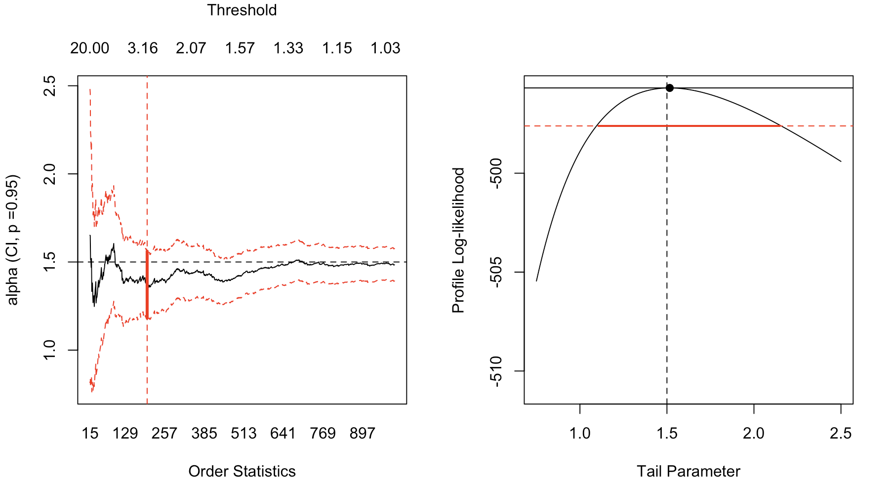
Figure 1: Hill estimator (on the left) for $\alpha$ and profile likelihood for $\alpha$ from a GPD model (on the right) on the top $20\%$ of the observations, when $n=1,000$ observations where generated from a (strict) Pareto distribution, with $\alpha=1.5$.

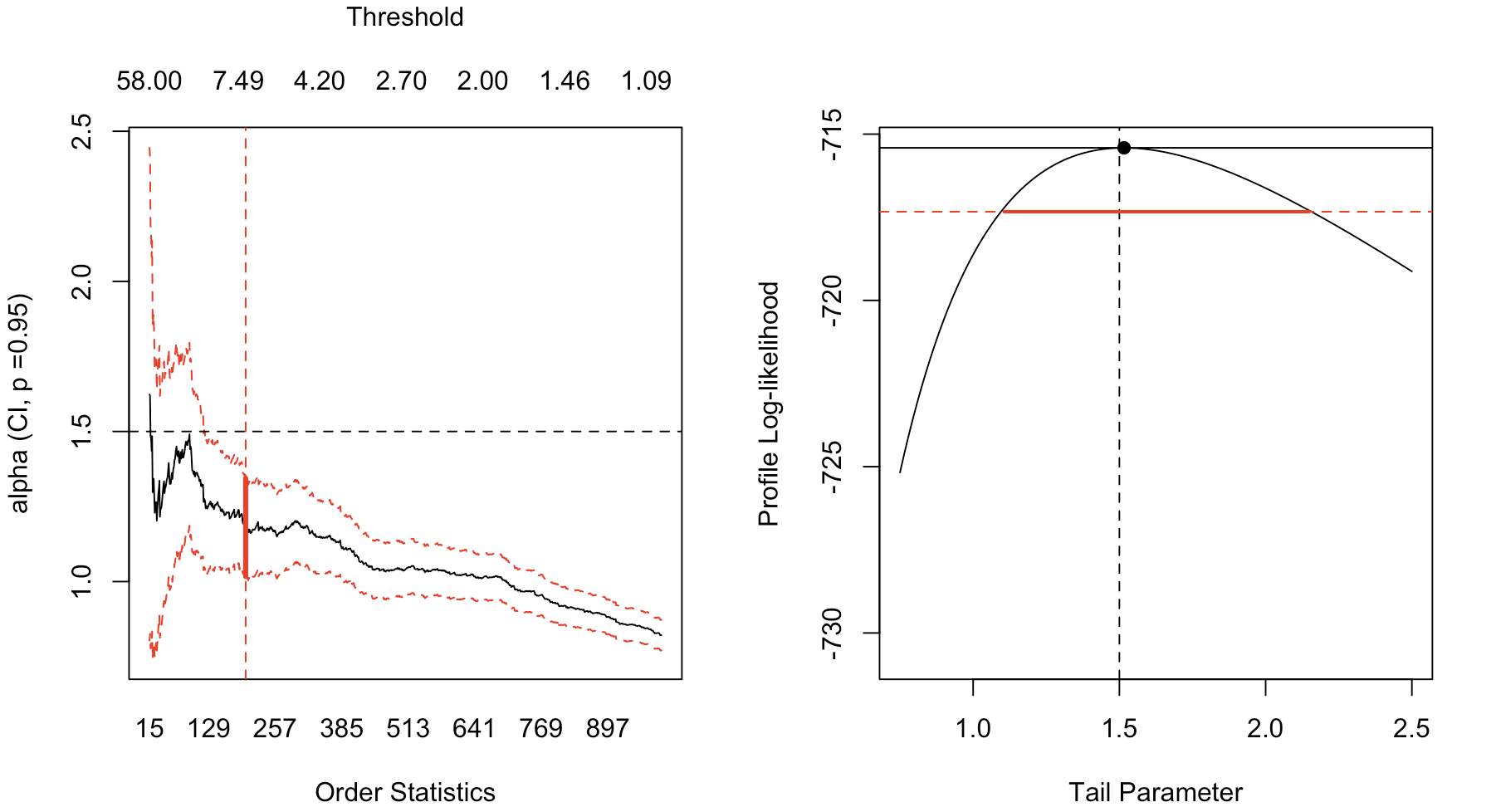
Figure 2: Hill estimator (on the left) for $\alpha$ and profile likelihood for $\alpha$ from a GPD model (on the right) on the top $20\%$ of the observations, when $n=1,000$ observations where generated from a Generalized Pareto distribution, with $\alpha=1.5$, and $\sigma=1$.

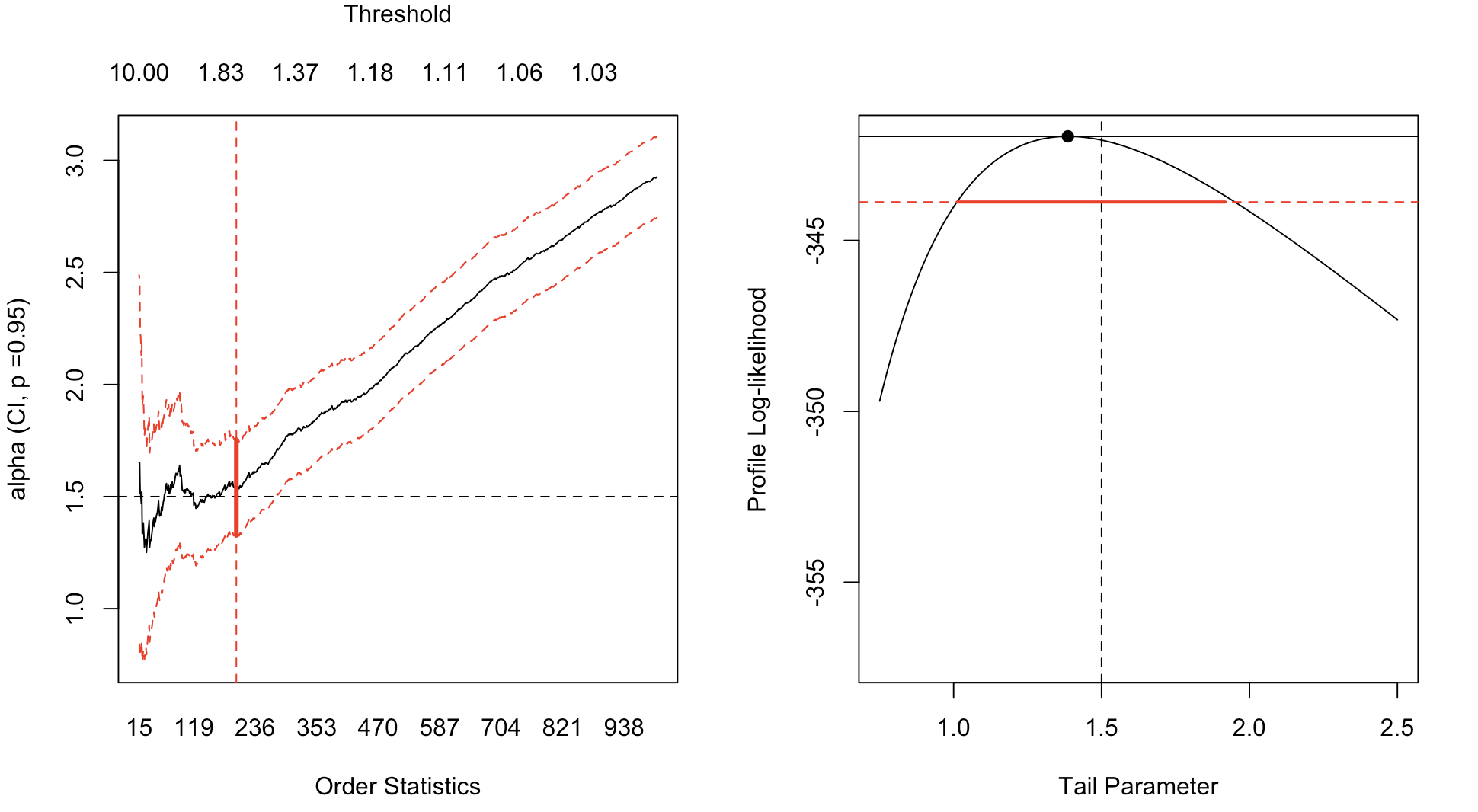
Figure 3: Hill estimator (on the left) for $\alpha$ and profile likelihood for $\alpha$ from a GPD model (on the right) on the top $20\%$ of the observations, when $n=1,000$ observations where generated from an extended Pareto distribution, with $\alpha=1.5$, and $\tau=-2$.

In the case of the EPD, the smaller the value of $\tau$, the more bias Hill estimator has (see CharpentierFlachaire for a detailed discussion). When generating a Pareto type distribution, using the top 80% observations does not guarantee anymore that Hill estimator could be a relevant estimator. On Figure 4, we used simulated samples of size $n=1,000$ with the same Monte Carlo seed (on the left), and another one (on the right), as on Figure 3, and we simply change the value of $\tau$. The red curve ( ) is Hill estimator $\widehat{\alpha}_{u}$ obtained when $u$ is the $60$% quantile, while the blue curve ( ) is obtained when $u$ is the $90$% quantile. The green curve ( ) is the profile likelihood estimator of a GPD distribution. Horizontal segments are confidence intervals. For Hill estimator, observe that if the threshold $u$ is not large enough, estimator can be substantially biased. For the GPD, the fit is better, but the confidence interval is very large. Observe further that when $\tau\in(-2,0)$, Hill estimator in the higher tail can actually be overestimated.

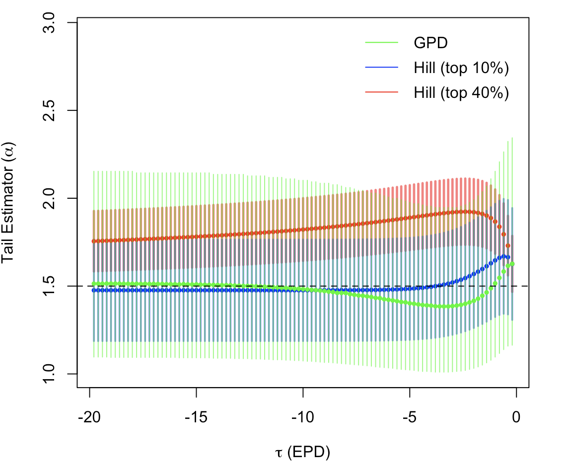
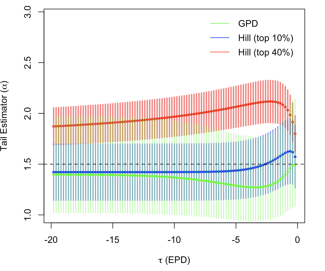
Figure 4: Simulation of EPD samples (with the same monte-carlo seed on the left, and another seed on the right), with $\alpha=1.5$, and $\tau$ varying from $-20$ to $0$. The red curve ( ) is Hill estimator $\widehat{\alpha}_{u}$ obtained when $u$ is the $60$% quantile, while the blue curve ( ) is obtained when $u$ is the 90% quantile. The green curve ( ) is the profile likelihood estimator of a GPD distribution.

5 Modeling large events

Given $n$ i.i.d. random losses $X_{1},\cdots,X_{n}$, let $S_{n}$ and $M_{n}$ respectively denote the sum and the maximum

$$S_{n}=X_{1}+\cdots+X_{n}\quad\text{ and }\quad M_{n}=\max\{X_{1},\cdots,X_{n}\}.$$ (44)

A classical concept is the Probable Maximum Loss (section 5.1) which is the distribution of $M_{n}$, or an affine transformation (since the distribution depends on $n$, the number of claims in insurance, or the time horizon in finance). It is possible, as in Section 3 of BeGoSeTe:04, to look “close to the maximum”, by studying the limiting distribution of the $k$-th largest value $X_{k:n}$, when $n$ goes to infinity, as well as $k$. If $k/n=O(1)$, we study the asymptotic distribution of some high quantile (Section 5.2). It is also possible to focus on large losses with respect to the entire portfolio, i.e. $S_{n}$. This will yield the concepts of Sub-Exponential distribution (section 5.3) when comparing $M_{n}$ and $S_{n}$, and comparing a high quantile, or the sum above a high quantile will be related to Top Share (section 5.4), also called Large Claim Index in insurance applications.

5.1 Probable Maximum Loss

Paul Levy extended the Central Limit Theorem to variables with a non-finite variance by considering non-degenerate distributions $G$ such that

$$\lim_{n\rightarrow\infty}\mathbb{P}\left(\frac{\overline{X}_{n}-b_{n}}{a_{n}}\leq x\right)=G(x)$$ (45)

where $\overline{X}_{n}=n^{-1}S_{n}$. It is an extension of the Central Limit Theorem in the sense that, if $X_{i}$’s have a finite variance and if $b_{n}=\mathbb{E}[X]$ while $a_{n}=\sqrt{n^{-1}\text{Var}[X]}$, then $G$ is the $\mathcal{N}(0,1)$ distribution, as well as any sequences such that $b_{n}\rightarrow\mathbb{E}[X]$ and $\sqrt{n}~{}a_{n}\rightarrow\sqrt{\text{Var}[X]}$, as $n\rightarrow\infty$. In the case of variables with infinite variance, then $G$ is called a stable distribution.

At the same period, Fisher-Tippett investigated a rather similar problem, searching for possible limiting distribution for a standardized version of the maximum

$$\lim_{n\rightarrow\infty}\mathbb{P}\left(\frac{M_{n}-b_{n}}{a_{n}}\leq x\right)=G(x).$$ (46)

It was shown - in Gnedenko:43 - that the only possible limit was the so-called extreme value distribution

$$G_{\alpha}(x)=\exp(-x^{-\alpha})$$ (47)

including the limiting case $G_{0}(x)=\exp(-e^{-x})$, on some appropriate interval. For instance, assume that $X$ is $\mathcal{P}({1,\alpha})$ distributed, let $b_{n}=0$ and $a_{n}=U(n)=n^{1/\alpha}$, then

$$\lim_{n\rightarrow\infty}\mathbb{P}\left(\frac{M_{n}-b_{n}}{a_{n}}\leq x\right) =\lim_{n\rightarrow\infty}\left[F(a_{n}x+b_{n})\right]^{n}=\lim_{n\rightarrow\infty}\left[F(n^{1/\alpha}x)\right]^{n}$$ (48)

$$=\lim_{n\rightarrow\infty}\left(1-\frac{x^{-\alpha}}{n}\right)^{n}=\exp(-x^{-\alpha})$$ (49)

More generally, assume that $X$ is Pareto type with tail index $\alpha$, and consider $b_{n}=0$ and $a_{n}\sim U(n)$ as $n\rightarrow\infty$. From Proposition 3.3.2 in EKM,

$$\lim_{n\rightarrow\infty}\left[F(a_{n}x+b_{n})\right]^{n}=\exp\left(\lim_{n\rightarrow\infty}-n\overline{F}(a_{n}x+b_{n})\right)$$ (50)

and since

$$n\overline{F}(a_{n}x)\sim\frac{\overline{F}(a_{n}x)}{\overline{F}(a_{n})}\rightarrow x^{-\alpha}\text{ as }n\rightarrow\infty$$ (51)

therefore, we can obtain

$$\lim_{n\rightarrow\infty}\mathbb{P}\left(\frac{M_{n}-b_{n}}{a_{n}}\leq x\right)=\exp(-x^{-\alpha})$$ (52)

as previously. Such a distribution is know as the Fréchet distribution with index $\alpha$.

5.2 High Quantiles and Expected Shorfall

Given a distribution $F$, the quantile of level $p$ of the distribution is

$$Q(p)=\inf\big{\{}y\in\mathbb{R}:F(y)\geq p\big{\}}.$$ (53)

Since we focus on high quantiles, i.e. $p\rightarrow 1$, a natural related function is

$$U(x)=Q\left(1-\frac{1}{x}\right),$$ (54)

and to study properties of that function as $x\rightarrow\infty$.

In the previous section, we studied limiting behavior of $a_{n}^{-1}(M_{n}-b_{n})$ as $n\rightarrow\infty$. Let $\widehat{F}_{n}$ denote the empirical cumulative distribution of $\{X_{1},\cdots,X_{n}\}$,

$$\widehat{F}_{n}(x)=\frac{1}{n}\sum_{i=1}^{n}\boldsymbol{1}(X_{i}\leq x).$$ (55)

Observe that $M_{n}=\widehat{F}_{n}^{-1}(1-1/n)=\widehat{U}_{n}(n)$, so $M_{n}$ should be ‘close’ to $U(n)$. So it could make sense to study

$$\lim_{n\rightarrow\infty}\frac{U(nx)-U(n)}{a_{n}}$$ (56)

BeJoSe:09 (BeJoSe:09, section 3.3) show that the only possible limit is

$$h(x)=\frac{x^{\gamma}-1}{\gamma}$$ (57)

If $U$ is the quantile function of $\mathcal{P}({1,\alpha})$, $U(x)=x^{1/\alpha}$, with auxiliary function $a(t)=\alpha^{-1}t^{1/\alpha}$, then

$$\frac{U(tx)-U(t)}{a(t)}=\alpha(x^{1/\alpha}-1)$$ (58)

for all $x$, i.e. $\gamma=\alpha^{-1}$.

Assume that $X$ is $\mathcal{P}({u,\alpha})$, then

$$Q(p)=u\cdot(1-p)^{-1/\alpha}$$ (59)

and if $X$ is $\mathcal{GPD}({u,\sigma,\alpha})$, then

$$Q(p)=u+\sigma\big{[}(1-p)^{-1/\alpha}-1\big{]}$$ (60)

For extended Pareto distributions quantiles are computed numerically.

Another important quantity is the average of the top $p\%$, called expected shortfall,

$$\text{ES}(p)=\mathbb{E}(X|X>Q(1-p))=\frac{1}{p}\int_{1-p}^{1}Q(u)du.$$ (61)

This quantity is closely related to the mean excess function, since $\text{ES}(p)=Q(1-p)+e(Q(1-p))$, where $e$ is the mean excess function. Assume that $X$ is $\mathcal{P}({u,\alpha})$, then

$$\text{ES}(p)=\frac{\alpha}{\alpha-1}u(1-p)^{-1/\alpha}=\frac{\alpha}{\alpha-1}Q(p),$$ (62)

and if $X$ is $\mathcal{GPD}({u,\sigma,\alpha})$, then $X|X>Q(1-p)$ is $\displaystyle{\mathcal{GPD}\left({Q(1-p),\sigma+Q(1-p)+u,\alpha}\right)}$ from Equation (15), and therefore

$$\text{ES}(p)=\frac{\alpha Q(1-p)+\sigma-u}{\alpha-1}.$$ (63)

For the extended Pareto model, only numerical approximations can be obtained.

On Figure 5 we have the evolution of $Q(1-p)$ for various values of $p$, from $1/10$ down to $1/1000$. A strict Pareto ( ) with tail index $\alpha=1.5$ is considered. On the left, we plot the quantile function of a GPD distribution ( ), for small and large $\sigma$’s, and on the right, we consider an EPD distribution ( ) with different values of $\tau$.

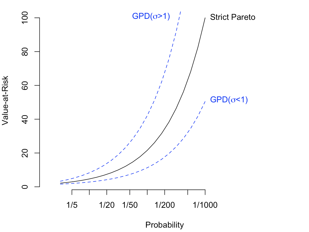
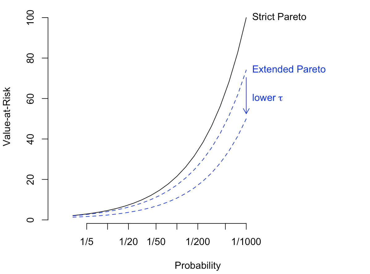
Figure 5: Quantile $Q(1-p)$ as a function of the probability $p$ (on a log scale), with a strict Pareto ( ) with tail index $\alpha=1.5$, and a GPD distribution ( ) on the left, and an EPD distribution ( ) on the right.

On Figure 6 we have the evolution of $ES(p)$ for various values of $p$, from $1/10$ down to $1/1000$. The strict Pareto distribution ( ) still has tail index $\alpha=1.5$. On the left, we plot the expected shortfall of a GPD distribution ( ), for small and large $\sigma$’s, and on the right, we consider an EPD distribution ( ) with different values of $\tau$.

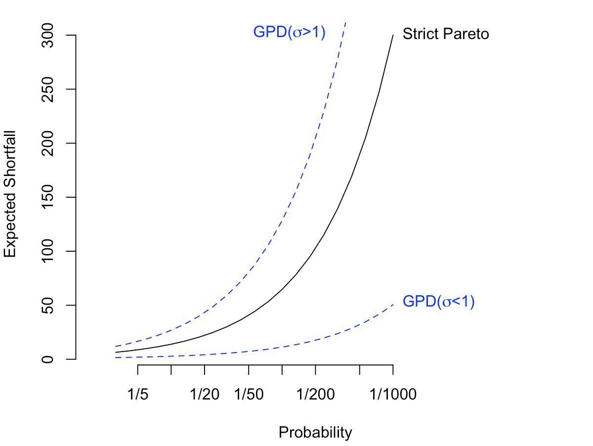
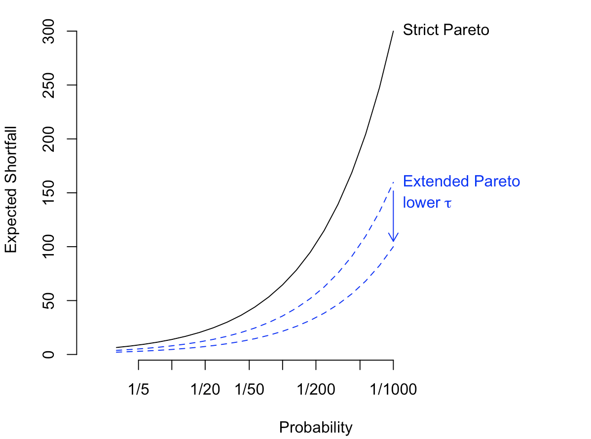
Figure 6: Expected Shortfall $\text{ES}(p)$ as a function of the probability (on a log scale), with a strict Pareto ( ) with tail index $\alpha=1.5$, and a GPD distribution ( ) on the left, and an EPD distribution ( ) on the right.

Finally, on Figure 7 we compare $Q(1-p)$ and $ES(p)$ for various values of $p$, and plot the line $(Q(1-p),ES(p))$. As expected, it is a straight line in the strict Pareto case ( ), above the first diagonal ( ), meaning that there can be substantial losses above any quantile. Two GPD distributions with the same tail index $\alpha$ are considered on the left ( ), and an EPD case is on the right ( ). The GPD case is not linear, but tends to be linear when $p$ is large enough (in the upper tail, we have a strict Pareto behavior). The EPD case is linear, with an Espected Shorfall smaller than the strict Pareto case.

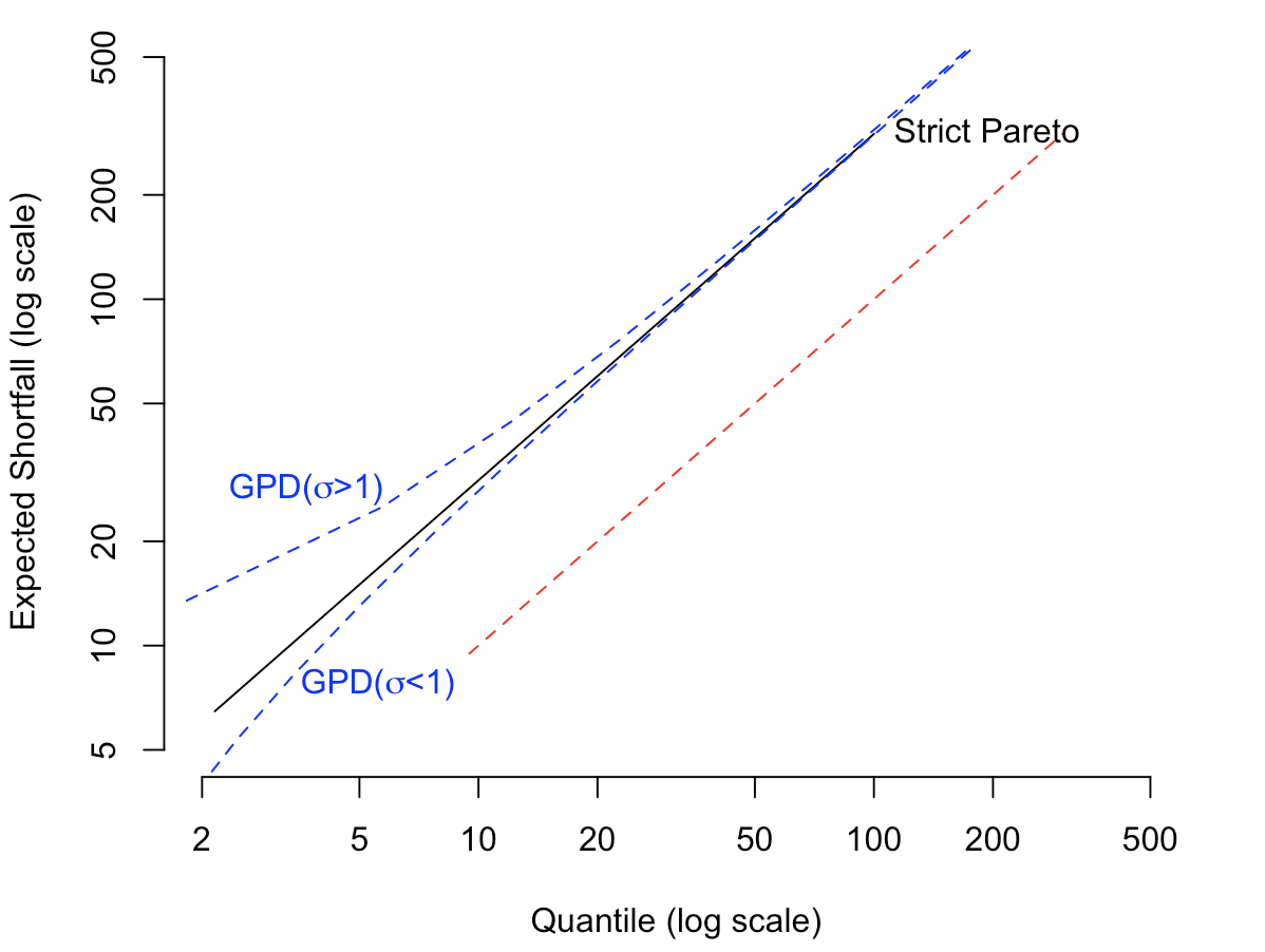
Figure 7: Expected Shortfall against quantile for different values of the probability (i.e. $(Q(1-p)),\text{ES}(p)$), with a strict Pareto ( ) with tail index $\alpha=1.5$, and a GPD distribution ( ) on the left, and an EPD distribution ( ) on the right. The straight line below ( ) is the identity curve, where the Expected Shortfall would be equal to the associated quantile.

5.3 Maximum, Sum and Subexponential distributions

In insurance, one possible way to define large losses is to say that a single claim is large when the total amount (over a given period of time) is predominantly determined by that single claim. The dominance of the largest value can be written

$$\mathbb{P}[S_{n}>x]\sim\mathbb{P}[M_{n}>x]\text{ as }x\rightarrow\infty.$$ (64)

Heuristically, the interpretation is that the sum will exceed a large value $x$ only when (at least) one single loss $X_{i}$ also exceeds $x$. If losses $X_{i}$ are i.i.d. with CDF $F$ we will say that $F$ belongs to the class of subsexponential distributions, $F\in\mathcal{S}$. As proved in AlBeTe:17 (AlBeTe:17, Section 3.2) strict Pareto and Pareto-type distributions belong to class $\mathcal{S}$. Hence, this class can be seen as an extension of the Pareto models. See goldie98 for applications of such distributions in a risk-management context.

In sections 6.2.6 and 8.2.4 of EKM, another quantity of interest is introduced, the ratio of the maximum and the sum, $M_{s}/S_{n}$. As proved in OBrien, $\mathbb{E}(X)$ is finite if and only if the ratio converges (almost surely) towards 0. A non-degenerated limit is obtained if and only if $X$ is Pareto type, with index $\alpha\in(0,1)$. An alternative would be to consider the ratio of the sum of the largest claims (and not only the largest one), and the total sum.

5.4 Top Share and Large Claim Index

In section 5.2, we discussed how to move from $M_{n}$ to the average of the top $p$% of the distribution. It could be possible to normalize by the total sum. The top $p$-% loss share can be defined as

$$\text{TS}(p)=\frac{p\,\mathbb{E}(X|X>Q(1-p))}{\mathbb{E}(X)}=\frac{p\text{ES}(p)}{\mathbb{E}(X)}=1-L(1-p)$$ (65)

where $L$ denote the Lorenz curve, i.e.

$$L(u)=\frac{1}{\mathbb{E}(X)}\int_{0}^{Q(u)}\overline{F}(y)dy=\frac{1}{\mathbb{E}(X)}\int_{0}^{u}Q(y)dy.$$ (66)

The empirical version of $\text{TS}_{p}$ is

$$\widehat{\text{TS}}(p)=\frac{x_{n-[np]:n}+x_{n:n}}{S_{n}}$$ (67)

where $(x_{i:n})$ denote the order version of sample $(x_{i})$, with $x_{1:n}\leq x_{2:n}\leq\cdots\leq x_{n:n}$. See section 8.2.2 of EKM for convergence properties of that estimator. In the case where $X$ is a strict Pareto $\mathcal{P}({u,\alpha})$, then

$$\text{TS}(p)=p^{(\alpha-1)/\alpha},$$ (68)

while if $X$ is $\mathcal{GPD}({u,\sigma,\alpha})$,

$$\text{TS}(p)=1-\frac{u(1-p)+\alpha\cdot\big{(}I_{1}(\alpha-2,2)-I_{p^{1/\alpha}(\alpha-1,2)}\big{)}}{u+\sigma\alpha I_{1}(\alpha-1,2)}$$ (69)

as in Section 6 of Arno:08PA, where $I_{z}(a,b)$ is the incomplete Beta function,

$$I_{z}(a,b)=\int_{0}^{z}t^{a-1}t^{(}1-t)^{b-1}dt.$$ (70)

No simple expression can be derive for the extended Pareto case, but numerical computations are possible, as on Figure 8, where strict Pareto distribution with tail index $\alpha=1.5$ is plotted against Pareto type distributions, GPD and EPD, with the same tail index.

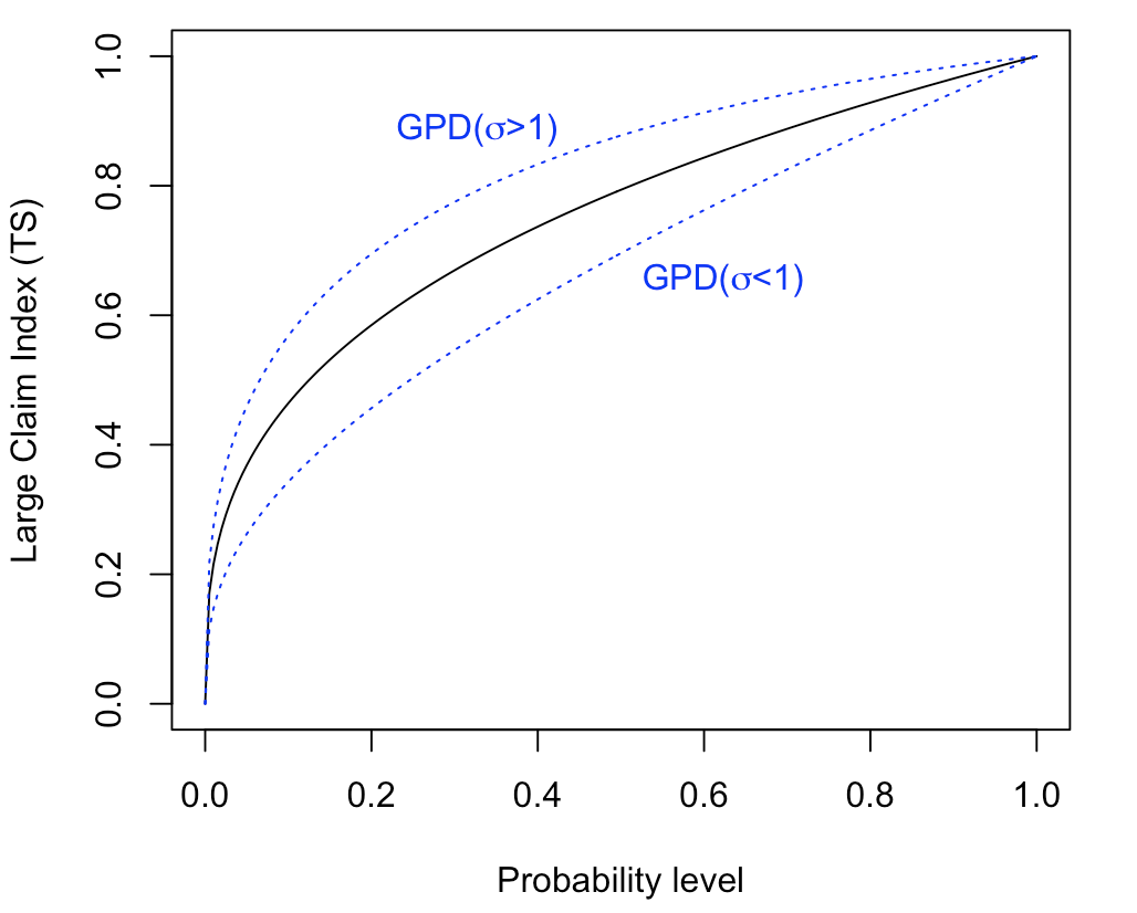
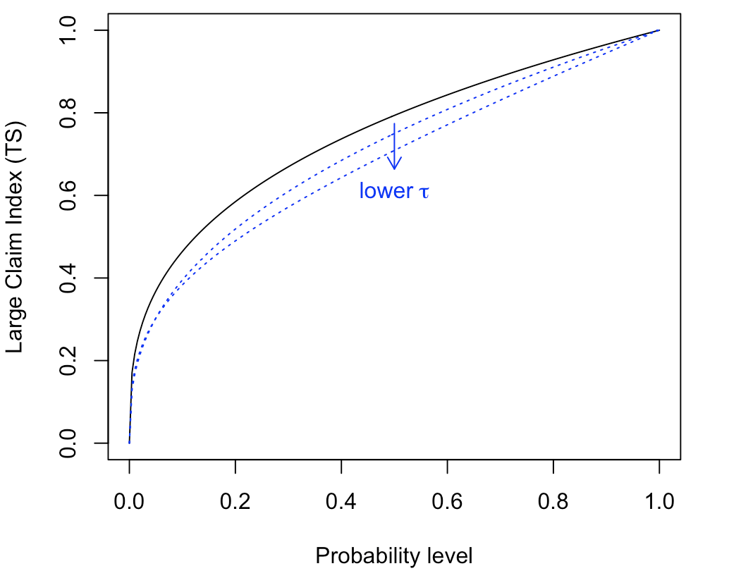
Figure 8: Large Claim Index $\text{TS}(p)$ as a function of the probability $p$, with a strict Pareto ( ) with tail index $\alpha=1.5$, and a GPD distribution ( ) on the left, and an EPD distribution ( ) on the right.

5.5 From Pareto to Pareto Type Models

The concepts introduced earlier were based on the assumption that the distribution $F$ of the observations was known. But actually, for small enough $p$, we might only have a Pareto distribution in the upper tail, above some threshold $u$, with $\mathbb{P}[X>u]\geq p$, as suggested in smith1987. And let $q_{u}$ denote the probability to exceed that threshold $q_{u}$.

Note that if $x>u$, $\mathbb{P}[X>x]=\mathbb{P}[X>x|X>u]\cdot\mathbb{P}[X>u]=q_{u}\mathbb{P}[X>x|X>u]$. Thus, if a $\mathcal{P}(u,\alpha)$ distribution is considered in the tails,

$$\mathbb{P}[X>x]=q_{u}\left(\frac{x}{u}\right)^{-\alpha}$$ (71)

and therefore,

$$Q_{u}(1-p)=u\cdot\left(\frac{p}{q_{u}}\right)^{-1/\alpha},\text{ where }q_{u}=\mathbb{P}[X>u],$$ (72)

and

$$\text{ES}_{u}(p)=\frac{\alpha}{\alpha-1}Q_{u}(1-p).$$ (73)

If a $\mathcal{GPD}(u,\sigma,\alpha)$ distribution is considered in the tails,

$$Q_{u}(1-p)=u\cdot\sigma\left[\left(\frac{p}{q_{u}}\right)^{-1/\alpha}-1\right]^{-1},\text{ where }q_{u}=\mathbb{P}[X>u],$$ (74)

and

$$\text{ES}_{u}(p)=\frac{\alpha Q_{u}(1-p)+\sigma-u}{\alpha-1}.$$ (75)

Nevertheless, if a simple update of formulas was necessary for downside risk measures (such as a quantile and an expected shortfall), expression can be more complicated when they rely on the entire distribution, such as the Large Claim Index TS. From Equation (65), if $p$ is small enough, write

$$\text{TS}_{u}(p)=\frac{p\text{ES}_{u}(p)}{\mathbb{E}(X)}$$ (76)

where $\mathbb{E}(X)$ is either approximated using $\overline{x}$, or a more robust version would be $(1-q_{u})\overline{x}_{u}+q_{u}\text{ES}_{u}(q_{u})$ where $\overline{x}_{u}$ is the empirical average of values below threshold $u$, while $\text{ES}_{u}(q_{u})$ is the parametric mean from a Pareto-type model, about threshold $u$.

6 Insurance and Reinsurance

Classical quantities in a reinsurance context are the return period (that can be related to quantiles, and the financial Value-at-Risk) and a stop-loss premium (related to the expected-shortfall).

6.1 Return Period and Return Level

Consider $Y_{1},\cdots,Y_{n}$, a collection of i.i.d. random variables, with distribution $F$. Consider the sequence of i.i.d. Bernoulli variables $X_{i}=\boldsymbol{1}_{Y_{i}>z(t)}$ for some threshold $z(t)$, such that $\overline{F}(z(t))=1/t$. The first time threshold $z(t)$ is reached is the random variable $N_{t}$ defined as

$$N_{t}=\min\big{\{}i\in\mathbb{N}_{*}:Y_{i}>z(t)\big{\}}.$$ (77)

Then $N_{t}$ has a geometric distribution,

$$\mathbb{P}\big{[}N_{t}=k\big{]}=\frac{1}{(1-t)^{k-1}}\frac{1}{t}.$$ (78)

The return period of the events $\{Y_{i}>z(t)\}$ is then $\mathbb{E}[N_{t}]=t$, or conversely, the threshold that is reached - on average - every $t$ events is $z(t)=Q(1-1/t)=U(t)$, called also return level.

Hence, with strict Pareto losses $\mathcal{P}(u,\alpha)$

$$z(t)=ut^{1/\alpha},$$ (79)

while with $\mathcal{GPD}({u,\sigma,\alpha})$ losses,

$$z(t)=u+\sigma\left[t^{1/\alpha}-1\right].$$ (80)

In the case of non-strict Pareto distribution, where only the top $q$% is $\mathcal{P}(u,\alpha)$ distributed,

$$z_{u}(t)=u(q_{u}t)^{1/\alpha},~{}\text{ where }~{}q_{u}=\mathbb{P}[X>u].$$ (81)

Thus, if we assume that the top $10\%$ is Pareto distributed, the return level of a centennial event ($t=100$) corresponds to the return level of a decennial event ($q_{u}t=10$) for the top $10\%$ observations. If the top $q$% is $\mathcal{GPD}(u,\sigma,\alpha)$ distributed,

$$z_{u}(t)=u+\sigma\big{(}(q_{u}t)^{1/\alpha}-1\big{)},~{}\text{ where }~{}q_{u}=\mathbb{P}[X>u].$$ (82)

From an empirical perspective, consider a dataset with $n$ observations, i.i.d., $y_{1},\cdots,y_{n}$. Assume that above threshold $u$, the (conditional) distribution is $\mathcal{GPD}({u,\sigma,\alpha})$. Denote $n_{u}$ the number of observations above $u$, so that $\widehat{F}_{n}(u)=1-n_{u}/n$. Then

$$\widehat{z}_{u}(t)=u+\widehat{\sigma}\left[\left(\frac{n_{u}}{n}t\right)^{1/\widehat{\alpha}}-1\right].$$ (83)

6.2 Reinsurance Pricing

Let $Y$ denote the loss amount of an accident. Consider a contract with deductible $d$, so that the indemnity paid by the insurance company is $(Y-d)_{+}$, where $\cdot_{+}$ denotes the positive part, i.e. $(y-d)_{+}=\max\{0,y-d\}$. The pure premium of such a contract, with deductible $d$, is

$$\pi(d)=\mathbb{E}\big{[}(Y-d)_{+}\big{]}$$ (84)

and therefore, if $e(d)$ denotes the mean excess function,

$$\pi(d)=\mathbb{E}\big{[}Y-d|Y>d\big{]}\cdot\mathbb{P}(Y>d)=e(d)\cdot\mathbb{P}(Y>d).$$ (85)

If we assume that losses above some threshold $u$ have a $\mathcal{GPD}(u,\sigma,\alpha)$ distribution, for any $d>u$,

$$e_{u}(d)=\left(\frac{\sigma-u}{\alpha-1}+\frac{\alpha}{\alpha-1}d\right)$$ (86)

and therefore

$$\pi_{u}(d)=\frac{n_{u}}{n}\left[1+\left(\frac{d-u}{\sigma}\right)\right]^{-\alpha}\cdot\left(\frac{\sigma-u}{\alpha-1}+\frac{\alpha}{\alpha-1}d\right).$$ (87)

If we plugin estimators of $\sigma$ and $\alpha$, we derive the estimator of the pure premium $\pi_{u}(d)$. Note that in Section 4.6. in AlBeTe:17, approximations are given for Extended Pareto distributions.

As previously, consider a dataset with $n$ observations, i.i.d., $y_{1},\cdots,y_{n}$, assume that above threshold $u$, the (conditional) distribution is $\mathcal{GPD}({u,\sigma,\alpha})$ and let $n_{u}$ denote the number of observations above $u$. Then if we fit a GPD distribution, the estimated premium would be

$$\widehat{\pi}_{u}(d)=\frac{n_{u}}{n}\left[1+\left(\frac{d-u}{\widehat{\sigma}}\right)\right]^{-\widehat{\alpha}}\cdot\left(\frac{\widehat{\sigma}-u}{\widehat{\alpha}-1}+\frac{{\alpha}}{\widehat{\alpha}-1}d\right),$$ (88)

for some deductible $d$, higher than $u$, our predefined threshold.

6.3 Application on Real Data

In order to illustrate, two datasets are considered, with a large fire loss dataset (the ‘Danish dataset’ studied in BeirlantTeugels1992 and McNeil:1997) and large medical losses (from the SOA dataset studied in cebrian2003). On Figure 9, Pareto plots are considered for losses above some threshold $u$, with $u=10$ for fire losses, and $u=1$ for medical losses (here in $\$^{\prime}00,000$), i.e.

$$\left(x_{i:n},1-\frac{i-(n-n_{u})}{n_{u}}\right)_{i=n-n_{u}+1,\cdots,n}$$ (89)

on a log-log scatterplot. In Pareto models, points should be on a straight line, with slope $-\alpha$. The plain line ( ) is the Pareto distribution (fitted using maximum likelihood techniques) and the dotted line ( ) corresponds to a Generalized Pareto distribution.

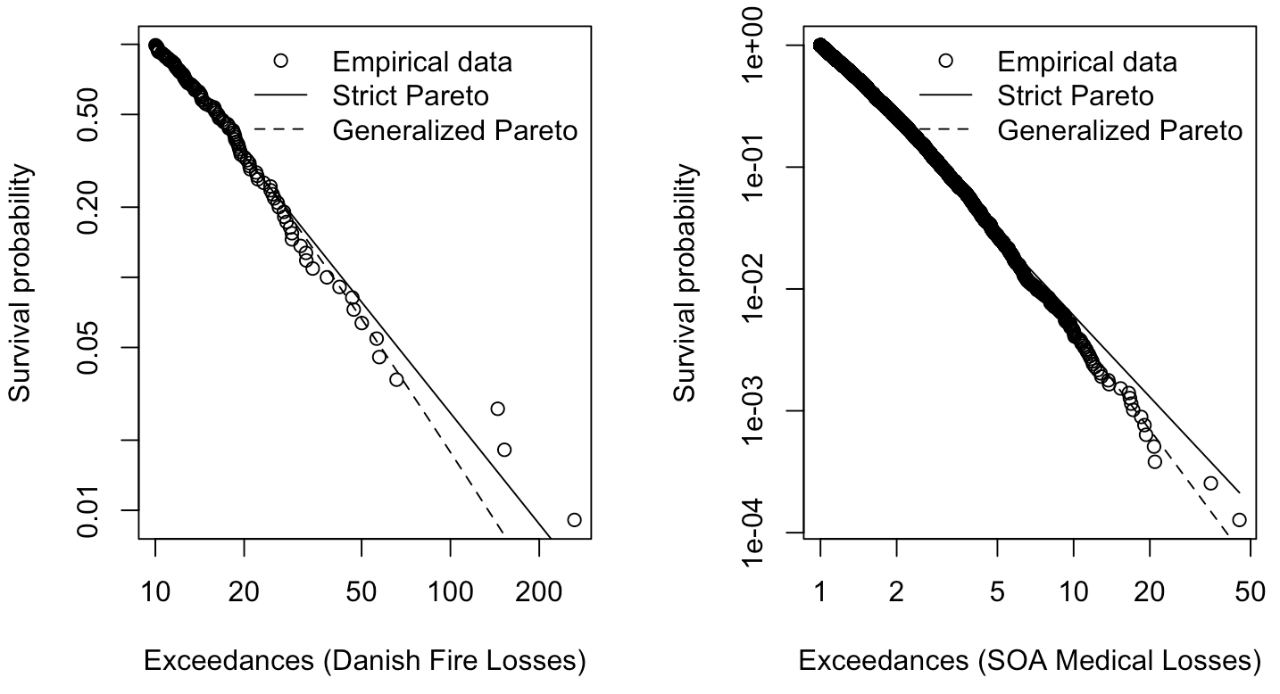
Figure 9: Pareto plot, with the Danish Fire data on the left, and the SOA Medical claims data on the right.

On Figure 10 we can visualize estimates of $\alpha$, as a function of the number of tail events considered. The strong line ( ) is the Pareto distribution, the thin line ( ) is the GPD distribution while the dotted line ( ) corresponds to a Extended Pareto distribution. Here the three distributions were fitted using maximum likelihood techniques, and only $\widehat{\alpha}$ is ploted.

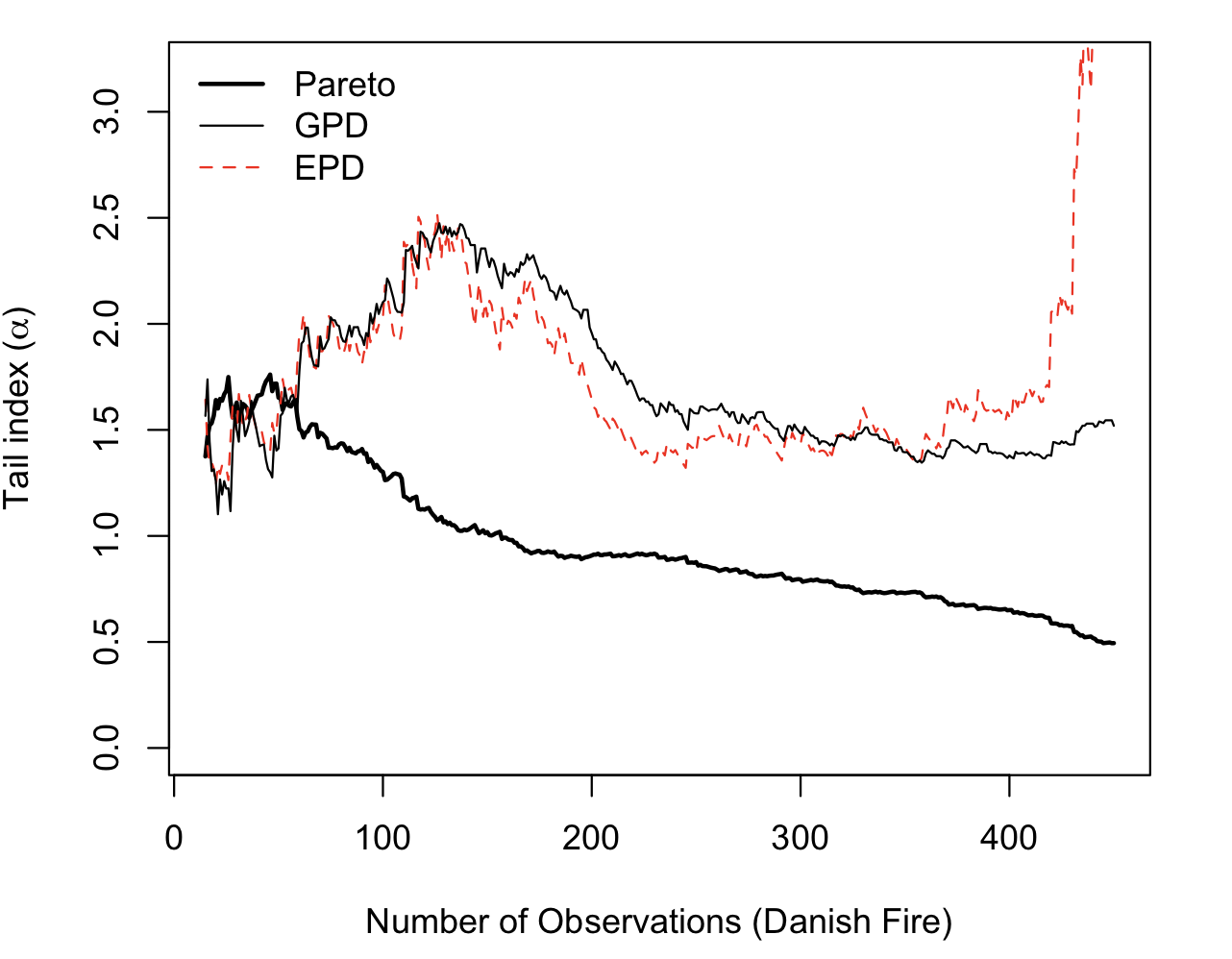
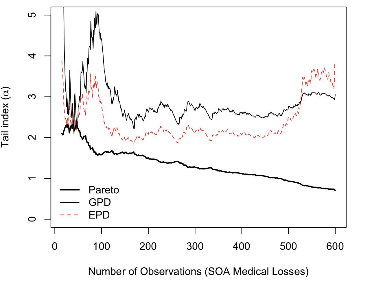
Figure 10: Estimation of $\alpha$, with a Pareto model ( ), a Generalized Pareto model ( ) and an Extended Pareto Model ( ), as a function of $n_{u}$, the number of tail events considered.

On Figure 11, we can visualize return levels for various return periods (on a log-scale), when Generalized Pareto distributions are fitted above level $u$ ($u=10$ for fires and $u=2$ for medical claims). Those values are quantiles, then return periods are interpreted as probabilities (e.g. a return period of 200 is a quantile of level $99.5\%$).

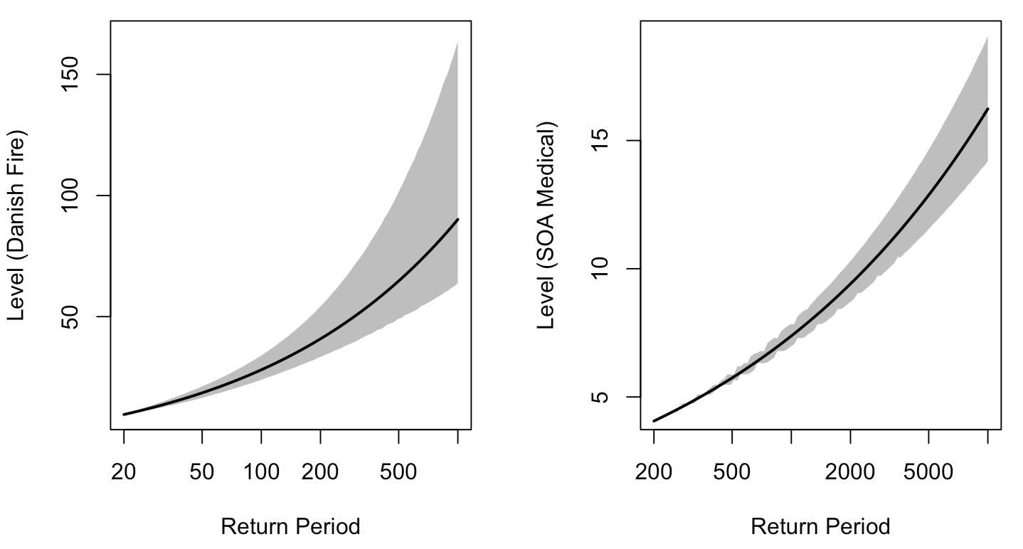
Figure 11: Estimation return levels for various return periods, for with the Danish Fire data on the left, and the SOA Medical claims data on the right. The grey area is the confidence region.

On Figure 12, we can visualize the mean excess function of individual claims, for fire losses on the left, and medical claims on the right (in $ ’00,000). The dark line is the empirical version (average above some threshold) and the line ( ) is the GPD fit

$$\widehat{e}_{u}(d)=\left(\frac{\widehat{\sigma}-u}{\widehat{\alpha}-1}+\frac{\widehat{\alpha}}{\widehat{\alpha}-1}d\right)$$ (90)

respectively with $u=10$ on the left and $u=2$ on the right, for various values of the threshold $d$ ($\geq u$).

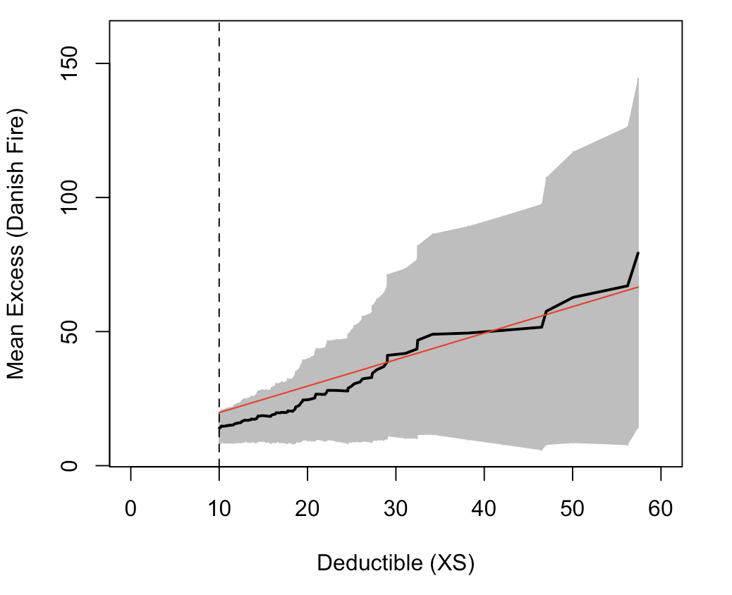
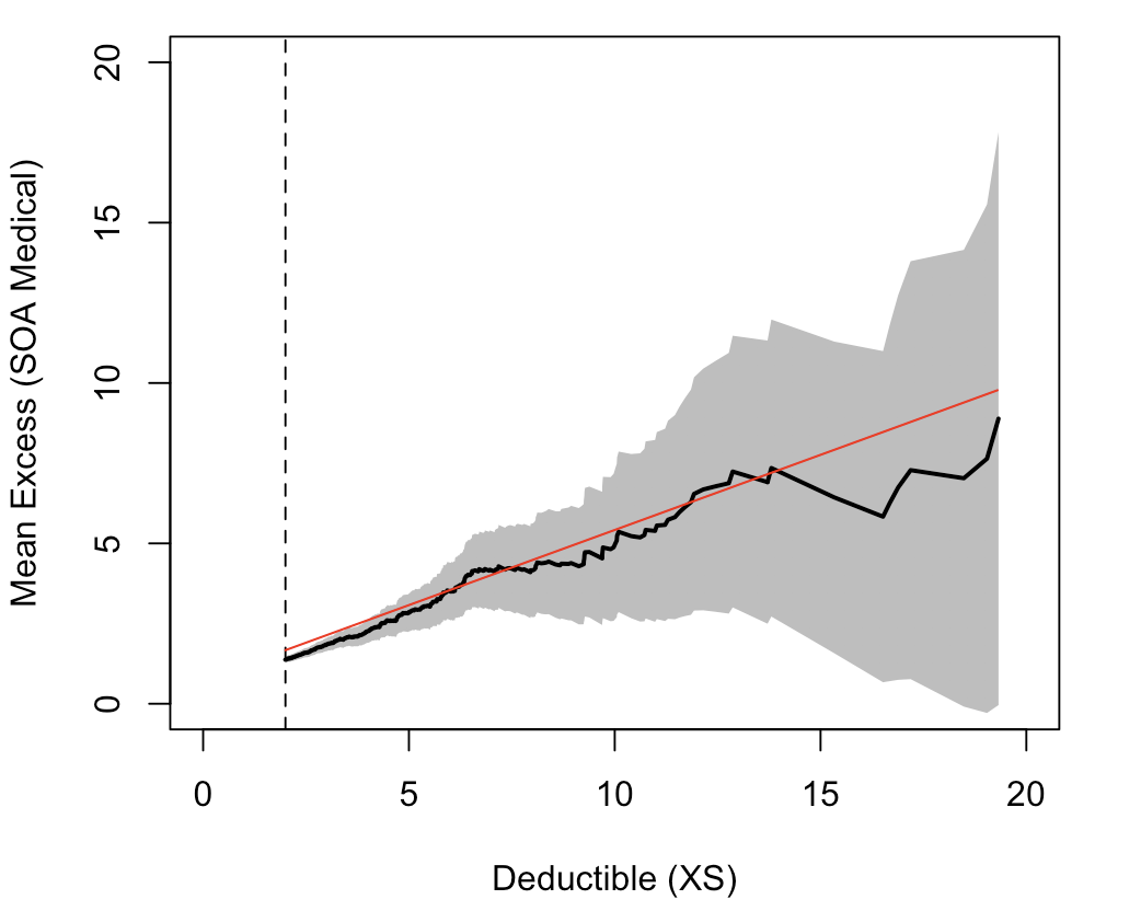
Figure 12: Mean excess functions Danish Fire data on the left, and the SOA Medical claims data on the right, with confidence intervals on the empirical version. The line ( ) is the GPD fit, for a given threshold (respectively 10 and 2).

On Figure 13, we can visualize the stability of estimators with respect to the choice of the threshold $u$, with the estimation of $e(d)$, with $d=20$ for Danish fires and $d=12$ for Medical losses. The empirical average is the horizontal dashed line ( ), the estimator derived from a Pareto distribution above threshold $u$ is the plain strong line ( ), the one from a Generalized Pareto model above threshold $u$ is the plain line ( ) and the Extended Pareto model above threshold $u$ is the dashed line ( ), as a function of $u$. The estimator obtained from the Extended Pareto model is quite stable, and close to the empirical estimate.

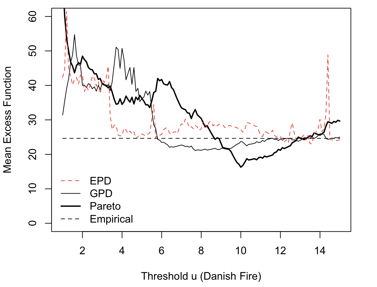
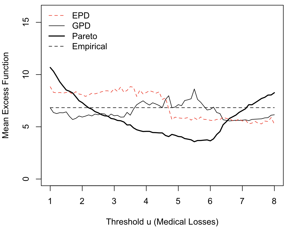
Figure 13: Estimation of $e(d)$, with $d=20$ for Danish fires and $d=12$ for Medical losses, with the empirical average ( ), the estimator derived from a Pareto distribution above threshold $u$ ( ), from a Generalized Pareto model above threshold $u$ ( ) and from an Extended Pareto Model above threshold $u$ ( ), as a function of $u$.

Finally, on Figure 14, we have the evolution of the (annual) pure premium, which is simply the mean excess function, multiplied by the (annual) probability to have a loss that exceed the deductible. For the Danish fire losses, since we have 10 years of data, the premium takes into account this 10 factor (which is consistent with a Poisson process assumption for claims occurrence): on average there are 11 claims per year above 10, and 2.5 above 25. For the SOA medical losses, there are 213 claims above $ 500,000 ($u=5$) for a mean excess function slightly below 3, so the pure premium is close to 600, for a deductible (per claim) of 5.

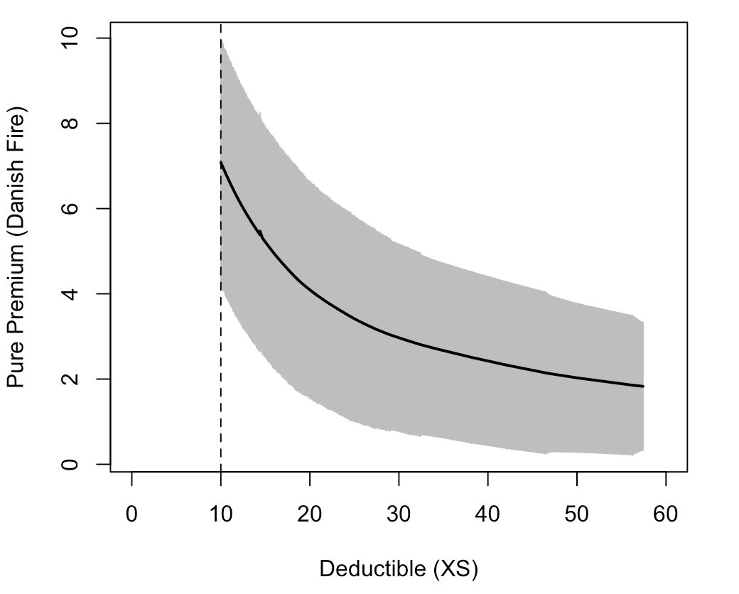
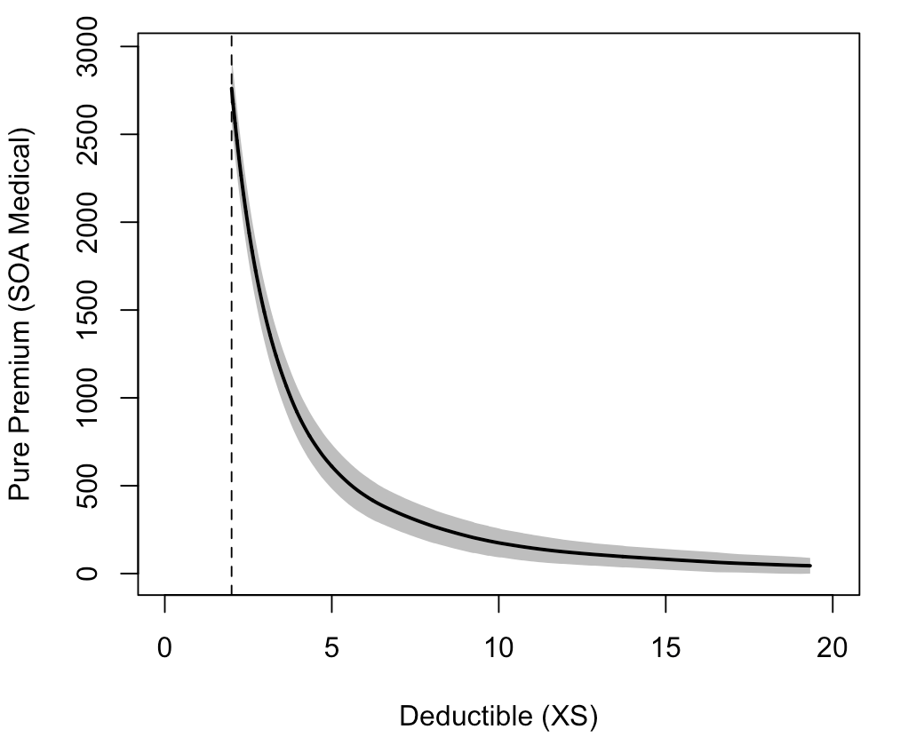
Figure 14: Annual Pure Premium for Danish Fire data on the left, and the SOA Medical claims data on the right.

7 Finance and risk-measures

7.1 Downside Risk Measures

Classical problems in risk management in financial applications involve (extreme) quantile estimation, such as the Value-at-Risk and the Expected Shortfall. Let $Y$ denote the negative returns of some financial instrument, then the Value-at-Risk $\text{VaR}(p)$ is defined as the quantile of level $1-p$ of the distribution,

$$\text{VaR}(p)=Q(1-p)=\inf\big{\{}y\in\mathbb{R}:F(y)\geq 1-p\big{\}},$$ (91)

while the expected shortfall (or tail conditional expectation) is the potential size of the loss exceeding the Value-at-Risk,

$$\text{ES}(p)=\mathbb{E}\big{[}X\big{|}X>\text{VaR}(p)\big{]}$$ (92)

If $X_{t}$ is the (random) loss variable of a financial position from time $t$ to time $t+h$ (with a given time horizon $h$), classical distributions have been intensively consider in financial literature, starting from the Gaussian case, $X_{t}\sim\mathcal{N}(\mu_{t},\Sigma_{t})$. Then

$$\text{VaR}(p)=\mu_{t}+\Phi^{-1}(1-p)\Sigma_{t}\quad\text{and}\quad\text{ES}_{p}=\mu_{t}+\frac{\phi(\Phi^{-1}(1-p))}{p}\Sigma_{t},$$ (93)

where $\phi$ and $\Phi$ denote respectively the density and the c.d.f. of the centered standard Gaussian distribution.

Since Pareto models have a simple expression to model losses above a threshold, with a GPD above a threshold $u$, for $y>u$,

$$\widehat{F}_{u}(y) =\mathbb{P}[Y\leq y]$$

$$=\mathbb{P}[Y\leq y|Y>u]\cdot\mathbb{P}[Y>u]+\mathbb{P}[Y\leq u]$$

$$=G_{\widehat{\sigma},\widehat{\alpha}}(y-u)\cdot\frac{n_{u}}{n}+\frac{n-n_{u}}{n}$$

where $n_{u}$ denotes the number of observations above threshold $u$, and

$$G_{\sigma,\alpha}(x)=1-\left[1+\left(\frac{x}{\sigma}\right)\right]^{-\alpha}\qquad\text{for }x\geq u,$$ (94)

is the $\mathcal{GPD}(0,\sigma,\alpha)$ CDF. Then for an event rare enough - i.e. a probability small enough ($p<n_{u}/n$) - the Value-at-Risk $\text{VaR}_{p}$ can be approximated by

$$\widehat{\text{VaR}}_{u}(p)=u\cdot\widehat{\sigma}\left[\left(\frac{p}{q_{u}}\right)^{-1/\widehat{\alpha}}-1\right]^{-1},\text{ where }q_{u}=\mathbb{P}[Y>u],$$ (95)

as well as the expected-shortfall,

$$\widehat{\text{ES}}_{u}(p)=\frac{\widehat{\alpha}\widehat{\text{VaR}}_{u}(p)+\widehat{\sigma}-u}{\widehat{\alpha}-1}.$$ (96)

7.2 Application on Real Data

In finance, log-returns are rarely independent, and it is necessary to take into account the dynamics of the volatility. Consider some GARCH-type process for log-returns, $y_{t}=\mu_{t}+\Sigma_{t}x_{t}$, where $(x_{t})$ are i.i.d. variables, and where $(\sigma_{t})$ is the stochastic volatility. Then, as mentioned in McNeilFrey2000

$$\widehat{\text{VaR}}_{Y_{t}|\Sigma_{t}}(p)=\mu_{t}+\Sigma_{t}\cdot\widehat{\text{VaR}}_{X_{t}}(p)$$ (97)

$$\widehat{\text{ES}}_{Y_{t}|\Sigma_{t}}(p)=\mu_{t}+\Sigma_{t}\cdot\widehat{\text{ES}}_{X_{t}}(p)$$ (98)

To estimate $(\Sigma_{t})$, several approaches can be considered, from the exponential weighted moving average (EWMA), with

$$\widehat{\Sigma}_{t+1}^{2}=\beta\widehat{\Sigma}_{t}+(1-\beta)y^{2}_{t},\text{ for some }\beta\in(0,1),$$ (99)

to the GARCH(1,1) process,

$$\widehat{\Sigma}_{t+1}^{2}=\alpha_{0}+\alpha_{1}y^{2}_{t}+\beta_{1}\widehat{\Sigma}_{t}\text{ for some }\alpha_{1},\beta_{1}\in(0,1),\text{ with }\alpha_{1}+\beta_{1}<1.$$ (100)

To illustrate, we use returns of the Brent crude price of oil, extracted from the North Sea prices and comprises Brent Blend, Forties Blend, Oseberg and Ekofisk crudes.

On Figure 15, for the plain line (GARCH+GPD, ) we use

$$\widehat{\text{VaR}}_{Y_{t}|\Sigma_{t}}(p)=\widehat{\Sigma}_{t}\cdot\widehat{\text{VaR}}_{X_{t}}(p)$$ (101)

where

$$\widehat{\text{VaR}}_{X_{t}}(p)=u+\frac{\widehat{\sigma}}{\widehat{\alpha}}\left[\left(\frac{n}{n_{u}}(1-q)\right)^{-\widehat{\alpha}}-1\right]$$ (102)

with $u=2\%$ and $\widehat{\Sigma}_{t}$ is the fitted volatility with a GARCH(1,1) process. The red line is obtained using a Generalized Pareto fit on a sliding window $[t\pm 150]$.

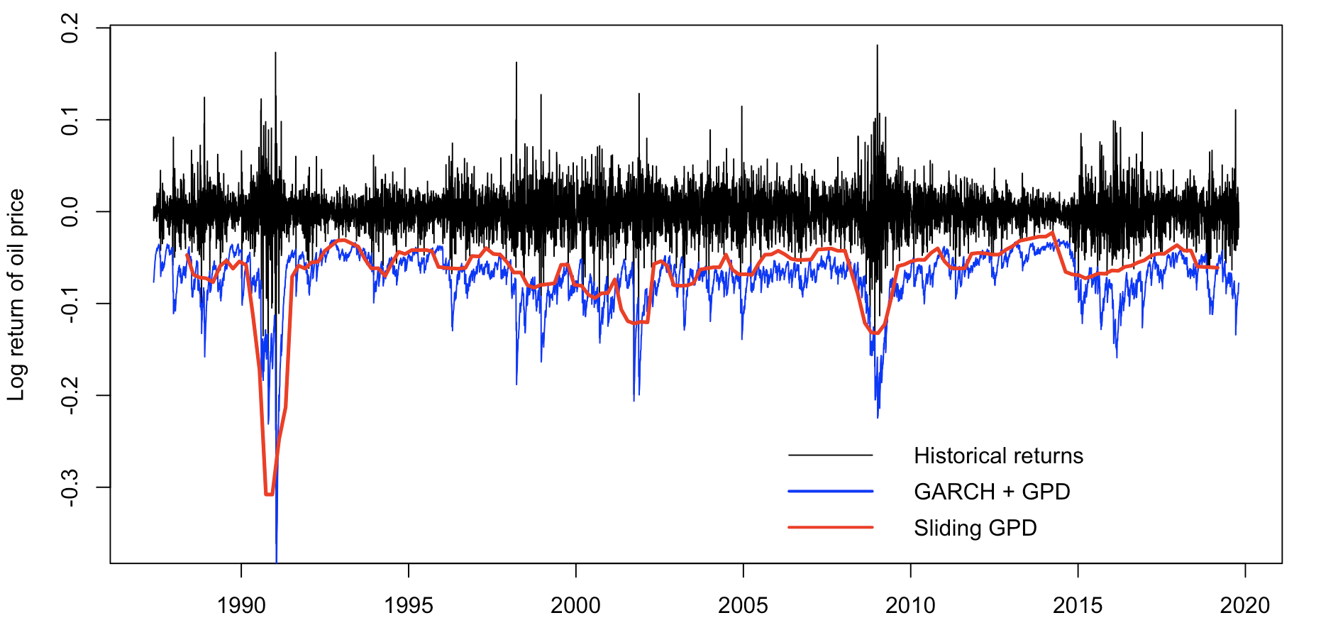
Figure 15: Value-at-Risk at level 0.5% for the daily log-return of oil prices ( ), with a GARCH+GPD model ( ) and a sliding window estimator GPD model ( )).

On Figure 16, an extended Pareto model is considered for $\widehat{\text{VaR}}_{X_{t}}(p)$.

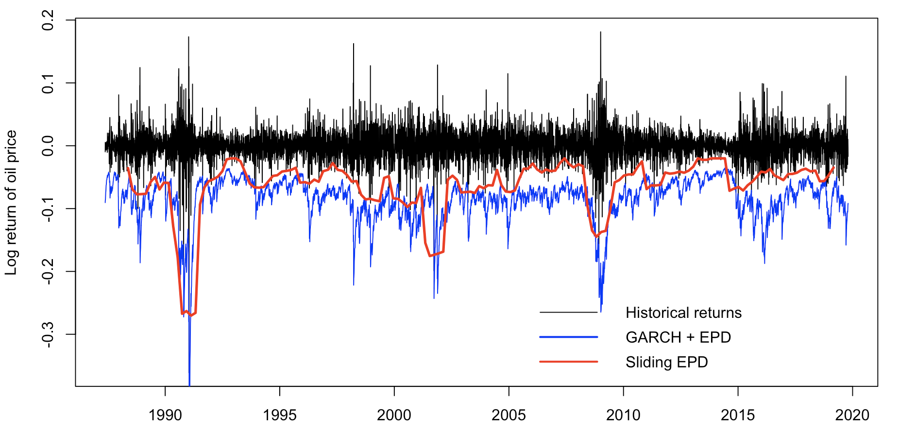
Figure 16: Value-at-Risk at level 0.5% for the daily log-return of oil prices ( ), with a GARCH+EPD model ( ) and a sliding window estimator EPD model ( ).

Finally, on Figure 17, we compare the GARCH + Pareto models, with either a Generalized Pareto model (as in McNeilFrey2000) or an Extended Pareto model. Observe that the 0.05% Value-at-Risk is always over estimated with the Generalized Pareto model. Nevertheless, with Pareto models estimated on sliding windows (on $[t\pm 150]$) the difference can be negative, sometimes. But overall, it is more likely that the Generalized Pareto overestimates the Value-at-Risk.

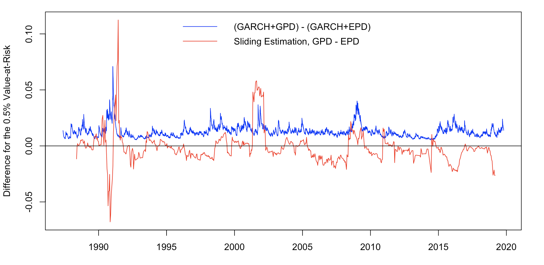
Figure 17: Difference of the Value-at-Risk at level 0.5% for the daily log-return of oil prices between GARCH+Pareto models ( ) and a sliding window estimator of Pareto models ( ).

References

- [\citeauthoryearAlbrecher, Beirlant, and TeugelsAlbrecher et al.2017] Albrecher, H., J. Beirlant, and J. L. Teugels (2017). Reinsurance: Actuarial and Statistical Aspects. Wiley Series in Probability and Statistics.
- [\citeauthoryearArnoldArnold2008] Arnold, B. C. (2008). Pareto and generalized Pareto distributions. In D. Chotikapanich (Ed.), Modeling Income Distributions and Lorenz Curves, Chapter 7, pp. 119–146. Springer.
- [\citeauthoryearBalkema and de HaanBalkema and de Haan1974] Balkema, A. and L. de Haan (1974). Residual life time at great age. Annals of Probability 2, 792–804.
- [\citeauthoryearBeirlant, Goegebeur, Segers, and TeugelsBeirlant et al.2004] Beirlant, J., Y. Goegebeur, J. Segers, and J. Teugels (2004). Statistics of Extremes: Theory and Applications. Wiley Series in Probability and Statistics.
- [\citeauthoryearBeirlant, Joossens, and SegersBeirlant et al.2009] Beirlant, J., E. Joossens, and J. Segers (2009). Second-order refined peaks-over-threshold modelling for heavy-tailed distributions. Journal of Statistical Planning and Inference 139, 2800–2815.
- [\citeauthoryearBeirlant and TeugelsBeirlant and Teugels1992] Beirlant, J. and J. L. Teugels (1992). Modeling large claims in non-life insurance. Insurance: Mathematics and Economics 11(1), 17 – 29.
- [\citeauthoryearBingham, Goldie, and TeugelsBingham et al.1987] Bingham, N. H., C. M. Goldie, and J. L. Teugels (1987). Regular Variation. Encyclopedia of Mathematics and its Applications. Cambridge University Press.
- [\citeauthoryearCebrián, Denuit, and LambertCebrián et al.2003] Cebrián, A. C., M. Denuit, and P. Lambert (2003). Generalized pareto fit to the society of actuaries’ large claims database. North American Actuarial Journal 7(3), 18–36.
- [\citeauthoryearCharpentier and FlachaireCharpentier and Flachaire2019] Charpentier, A. and E. Flachaire (2019). Pareto models for top incomes. hal id: hal-02145024.
- [\citeauthoryearDavisonDavison2003] Davison, A. (2003). Statistical Models. Cambridge University Press.
- [\citeauthoryearde Haan and Ferreirade Haan and Ferreira2006] de Haan, L. and A. Ferreira (2006). Extreme Value Theory: An introduction. Springer Series in Operations Research and Financial Engineering.
- [\citeauthoryearde Haan and Stadtmüllerde Haan and Stadtmüller1996] de Haan, L. and U. Stadtmüller (1996). Generalized regular variation of second order. Journal of the Australian Mathematical Society 61, 381–395.
- [\citeauthoryearEmbrechts, Klüppelberg, and MikoschEmbrechts et al.1997] Embrechts, P., C. Klüppelberg, and T. Mikosch (1997). Modelling Extremal Events for Insurance and Finance. Berlin Heidelberg: Springer-Verlag.
- [\citeauthoryearFisher and TippettFisher and Tippett1928] Fisher, R. A. and L. H. C. Tippett (1928). Limiting forms of the frequency distribution of the largest or smallest member of a sample. In Proceedings of the Cambridge Philosophical Society, Volume 24, pp. 180–290.
- [\citeauthoryearGabaixGabaix2009] Gabaix, X. (2009). Power laws in economics and finance. Annual Review of Economics 1(1), 255–294.
- [\citeauthoryearGhosh and ResnickGhosh and Resnick2010] Ghosh, S. and S. Resnick (2010). A discussion on mean excess plots. Stochastic Processes and their Applications 120(8), 1492 – 1517.
- [\citeauthoryearGnedenkoGnedenko1943] Gnedenko, B. (1943). Sur la distribution limite du terme maximum d’une serie aleatoire. Annals of Mathematics 44(3), 423–453.
- [\citeauthoryearGoldie and KlüppelbergGoldie and Klüppelberg1998] Goldie, C. M. and C. Klüppelberg (1998). Subexponential distributions. In R. J. Adler, R. E. Feldman, and M. S. Taqqu (Eds.), A Practical Guide to Heavy Tails, pp. 436–459. Birkhäuser.
- [\citeauthoryearGuess and ProschanGuess and Proschan1988] Guess, F. and F. Proschan (1988). 12 mean residual life: Theory and applications. In Quality Control and Reliability, Volume 7 of Handbook of Statistics, pp. 215 – 224. Elsevier.
- [\citeauthoryearHagstroemHagstroem1925] Hagstroem, K. G. (1925). La loi de pareto et la reassurance. Skandinavisk Aktuarietidskrift 25.
- [\citeauthoryearHagstroemHagstroem1960] Hagstroem, K. G. (1960). Remarks on pareto distributions. Scandinavian Actuarial Journal 60(1-2), 59–71.
- [\citeauthoryearHallHall1982] Hall, P. (1982). On some simple estimate of an exponent of regular variation. Journal of the Royal Statistical Society: Series B 44, 37–42.
- [\citeauthoryearJessen and MikoschJessen and Mikosch2006] Jessen, A. H. and T. Mikosch (2006). Regularly varying functions. Publications de l’Institut Mathématique 19, 171 – 192.
- [\citeauthoryearKlüppelbergKlüppelberg2004] Klüppelberg, C. (2004). Risk management with extreme value theory. In B. Finkenstädt and H. Rootzén (Eds.), Extreme Values in Finance, Telecommunications, and the Environment, Chapter 3, pp. 101–168. Oxford: Chapman & Hall/CRC.
- [\citeauthoryearKremerKremer1984] Kremer, E. (1984). Rating of Non Proportional Reinsurance Treaties Based on Ordered Claims, pp. 285–314. Dordrecht: Springer Netherlands.
- [\citeauthoryearLomaxLomax1954] Lomax, K. S. (1954). Business failures: Another example of the analysis of failure data. Journal of the American Statistical Association 49(268), 847–852.
- [\citeauthoryearMcNeilMcNeil1997] McNeil, A. (1997). Estimating the tails of loss severity distributions using extreme value theory. ASTIN Bulletin 27(27), 117–137.
- [\citeauthoryearMcNeil and FreyMcNeil and Frey2000] McNeil, A. J. and R. Frey (2000). Estimation of tail-related risk measures for heteroscedastic financial time series: an extreme value approach. Journal of Empirical Finance 7(3), 271 – 300. Special issue on Risk Management.
- [\citeauthoryearO’BrienO’Brien1980] O’Brien, G. L. (1980). A limit theorem for sample maxima and heavy branches in galton-watson trees. Journal of Applied Probability 17(2), 539–545.
- [\citeauthoryearParetoPareto1895] Pareto, V. (1895). La legge della domanda. In Pareto (Ed.), Ecrits d’économie politique pure, Chapter 11, pp. 295–304. Genève: Librairie Droz.
- [\citeauthoryearPeng and QiPeng and Qi2004] Peng, L. and Y. Qi (2004). Estimating the first- and second-order parameters of a heavy-tailed distribution. Australian & New Zealand Journal of Statistics 46, 305–312.
- [\citeauthoryearPickandsPickands1975] Pickands, J. (1975). Statistical inference using extreme order statistics. Annals of Statistics 23, 119–131.
- [\citeauthoryearResnickResnick1997] Resnick, S. I. (1997). Discussion of the danish data on large fire insurance losses. ASTIN Bulletin 27(1), 139–151.
- [\citeauthoryearResnickResnick2007] Resnick, S. I. (2007). Heavy-Tail Phenomena: Probabilistic and Statistical Modeling. Springer Series in Operations Research and Financial Engineering.
- [\citeauthoryearReynkensReynkens2018] Reynkens, T. (2018). ReIns: Functions from “Reinsurance: Actuarial and Statistical Aspects”. R package version 1.0.8.
- [\citeauthoryearRigby and StasinopoulosRigby and Stasinopoulos2005] Rigby, R. A. and D. M. Stasinopoulos (2005). Generalized additive models for location, scale and shape,(with discussion). Applied Statistics 54, 507–554.
- [\citeauthoryearRoyRoy1952] Roy, A. D. (1952). Safety first and the holding of assets. Econometrica 20(3), 431–449.
- [\citeauthoryearSchumpeterSchumpeter1949] Schumpeter, J. A. (1949). Vilfredo pareto (1848–1923). The Quarterly Journal of Economics 63(2), 147–173.
- [\citeauthoryearScollnikScollnik2007] Scollnik, D. P. M. (2007). On composite lognormal-pareto models. Scandinavian Actuarial Journal 2007(1), 20–33.
- [\citeauthoryearSmithSmith1987] Smith, R. L. (1987, 09). Estimating tails of probability distributions. Ann. Statist. 15(3), 1174–1207.
- [\citeauthoryearVajdaVajda1951] Vajda, S. (1951). Analytical studies in stop-loss reinsurance. Scandinavian Actuarial Journal 1951(1-2), 158–175.