A statistical test for correspondence of texts to the Zipf—Mandelbrot law

Abstract

We analyse correspondence of a text to a simple probabilistic model. The model assumes that the words are selected independently from an infinite dictionary. The probability distribution correspond to the Zipf—Mandelbrot law. We count sequentially the numbers of different words in the text and get the process of the numbers of different words. Then we estimate Zipf—Mandelbrot law parameters using the same sequence and construct an estimate of the expectation of the number of different words in the text. Then we subtract the corresponding values of the estimate from the sequence and normalize along the coordinate axes, obtaining a random process on a segment from 0 to 1. We prove that this process (the empirical text bridge) converges weakly in the uniform metric on $C(0,1)$ to a centered Gaussian process with continuous a.s. paths. We develop and implement an algorithm for approximate calculation of eigenvalues of the covariance function of the limit Gaussian process, and then an algorithm for calculating the probability distribution of the integral of the square of this process. We use the algorithm to analyze uniformity of texts in English, French, Russian and Chinese.

1 Introduction

Our analysis is based on the fact that a text in any natural language can be divided into words. The source material for our analysis is a text in which words are separated and punctuation marks are excluded. In addition, all capital letters (if any) are replaced by lowercase.

We test the hypothesis $H$ that a text matches a simple probabilistic model. This model is:

1) the potential number of different words (the volume of the dictionary) is infinitely large;

2) words are selected from the dictionary independently of each other with the same discrete probability distribution;

3) this probability distribution has a very specific form: if we arrange an infinite dictionary according to word probabilities, then the probability of occurrence of a word with number $i$ is

$$p_{i}=c(i+q)^{-\alpha},\ \ i\geq 1,\ \ \alpha=1/\theta,\ \ 0<\theta<1,\ \ q>-1.$$ (1)

$c>0$ is a normalizing constant ensuring equality of the sum of the probabilities to 1.

These assumptions have a long history. Power-law character of decay of probabilities together with the infinity of the dictionary proposed by Zipf (1936). Mandelbrot (1965) noted that shift $q$ is required to better match real texts. Modern large-scale studies (see Petersen et al., 2012) show that the process of the emergence of new words never stops, but very long sequences of texts show a slightly lower frequency of new words than this is predicted by the formula (1). Therefore, we will test the hypothesis $H$ for not very long texts. (less than $10^{5}$ words). We will demonstrate an example of non-correspondence of a long text to the hypothesis $H$.

The second assumption of the independence of the choice of consecutive words is obviously false for any meaningful text. We can easily reject it statistically. If we calculate the relative frequency of the word and in an English text, and then the relative frequency of the sequence and and (that is, two and in succession), then, according to $H$, the second should be approximately equal to the square of the first. In practice, the second is much smaller, often it is simply zero.

But we are not ready to abandon the assumption of independence. This assumption is a base of our analysis. Therefore, we choose a characteristic that changes little when rearranging neighboring words. This is the number of different words of the text, more precisely, a sequence of numbers of different words of the text $R_{1},\ldots,R_{n}$. Under this assumption of independence, Bahadur proved the law of large numbers $R_{n}/{\bf E}R_{n}\to 1$ in probability, and Karlin proved strong law of large numbers $R_{n}/{\bf E}R_{n}\to 1$ a.s. and the central limit theorem: $(R_{n}-{\bf E}R_{n})/\sqrt{{\bf Var}R_{n}}$ converges weakly to the standard normal law.

Thus, we consider a text as a random sequence, we construct the sequence $R_{1},\ldots,R_{n}$ and study it using the methods of the theory of random processes: we invent parameter estimates and construct the empirical text bridge, that is, a random process built on the parameter estimates and the sequence of numbers of different words. We find the limit Gaussian process in the sense of weak convergence in $C(0,1)$. Then we calculate the distribution function $G$ of the integral of the squared limit process based on the Smirnov (1937) formula.

Eigenvalues of the covariance function that are necessary for applying the Smirnov formula are calculated approximately as the eigenvalues of the matrix $Q=(q_{ij})_{i,j=1}^{100}$ composed of coefficients

$$q_{ij}=\int_{0}^{1}\int_{0}^{1}\widehat{K}(s,t)\sin\pi is\sin\pi jt\,dsdt.$$ (2)

We calculate $q_{ij}$ by a fast algorithm that reduces double integrals to definite integrals.

Asymptotics of $R_{n}$ and similar statistics (in particular, the number of unique words, that is, words with exactly one occurrence in the text) have been studied by a number of authors. The Gaussian approximation under assumptions (1) was studied by Karlin, and beyond these assumptions by Dutko (1989), Gnedin, Hansen and Pitman (2007), Hwang and Janson (2008), Barbour and Gnedin (2009). Barbour (2009) proposed translated Poisson approximation for the number of unique words. New papers by Ben-Hamou, Boucheron and Ohannessian (2017) and Decrouez, Grabchak and Paris (2018) proved new general facts about these statistics.

The main result on which our study is based is the functional central limit theorem for the sequence $R_{1},\ldots,R_{n}$. It was proven by Chebunin and Kovalevskii (2016) in preparation for this study. Note that the Gaussian process which is the limit for this sequence can be found also in Durieu and Wang (2016) as a limit for another prelimit process. Its generalization is in Durieu, Samorodnitsky and Wang (2019).

Zipf parameter estimates were proposed by Nicholls (1987), Chebunin and Kovalevskii (2019b), but we need a special estimate for which we can calculate joint limit distribution of it and of the sequence $R_{1},\ldots,R_{n}$. This estimate is proposed in Chebunin and Kovalevskii (2019a). Zakrevskaya and Kovalevskii (2019) used the estimate in analysis of Shakespeare’s sonnets.

Bahadur proved that under $H$ the mathematical expectation of the number of different words grows according to an asymptotically power law. This fact is known to experts in natural language processing as Herdan’s law (Herdan, 1960) or Heaps’ law (Heaps, 1978). Van Leijenhorst and van der Weide (2005), Eliazar (2011) analyzed the relationship between the Zipf’s law and Heaps’ law based on probabilistic models that were different from $H$.

Gerlach and Altmann (2013) noted specifically that there is no mathematically correct statistical test for correspondence of a text to the Zipf’s law. We proposed such a test in Chebunin and Kovalevskii (2019a). We are developing the algorithm and applying it to texts in different languages in the present paper.

The rest of the paper is organised as follows. The neccessary theoretical results are in Section 2, the algorythm is in Section 3, and results of text analysis are in Section 4. Proofs and calculation of matrix $Q$ are in Appendixes 1 and 2.

2 Theoretical results

Note that constant $c$ in (1) is

$$c=\left(\zeta(\alpha,q+1)\right)^{-1},$$

$$\zeta(\alpha,x)=\sum_{i=0}^{\infty}(i+x)^{-\alpha}$$

is Hurvitz zeta function.

Let $n$ be a number of words in a text.

Let $R_{k}$ be the number of different words among first $k$ words of the text.

Let $R_{0}=0$. We have $R_{1}=1$, $R_{0}<R_{1}\leq R_{2}\leq\ldots\leq R_{n}$.

Bahadur (1960) proved that

$${\bf E}R_{j}\sim c^{\theta}\Gamma(1-\theta)j^{\theta},$$ (3)

where $\Gamma(x)=\int_{0}^{\infty}y^{x-1}e^{-y}\,dy$ is the Euler gamma function. Bahadur also proved convergence in probability $R_{j}/{\bf E}R_{j}\stackrel{{\scriptstyle p}}{{\to}}1$.

Karlin (1967) proved that $R_{j}/{\bf E}R_{j}\stackrel{{\scriptstyle a.s.}}{{\to}}1$, which is equivalent to

$$R_{j}\sim C_{1}j^{\theta}\ {\rm a.s.,}$$ (4)

thanks to (3). Here $C_{1}=c^{\theta}\Gamma(1-\theta)$, coefficients $c$ and $\theta$ are from (3).

Chebunin and Kovalevskii (2016) proved the Functional Central Limit Theorem, that is, the weak convergence of the process $\{(R_{[nt]}-{\bf E}R_{[nt]})/\sqrt{{\bf E}R_{n}},\ 0\leq t\leq 1\}$ to a centered Gaussian process $Z$ with continuous a.s. sample paths and covariance function of the form

$$K(s,t)=(s+t)^{\theta}-\max(s^{\theta},t^{\theta}).$$

We propose the following estimator for parameter $\theta$ (Chebunin and Kovalevskii, 2019a)

$$\widehat{\theta}=\int_{0}^{1}\log^{+}R_{[nt]}\,dA(t)$$

with function $A(\cdot)$ such that

$$\int_{0}^{1}\log t\,dA(t)=1,\ \ A(0)=A(+0)=A(1)=0,$$ (5)

here $\log^{+}x=\max(\log x,\,0)$. We assume $A(\cdot)$ to be the sum of a step function and a piecewise continuosly differentiable function on $[0,\,1]$. Let $A(t)=0$, $t\in[0,\,\delta]$ for some $\delta\in(0,\,1)$.

The next theorem follows from Theorems 2.1, 2.2 by Chebunin and Kovalevskii (2019a).

Theorem 2.1 The estimator $\widehat{\theta}$ is strongly consistent, and

$$\sqrt{{\bf E}R_{n}}(\widehat{\theta}-\theta)-\int_{0}^{1}t^{-\theta}Z_{n}(t)\,dA(t)\to_{p}0.$$

From Theorem 2.1, it follows that $\widehat{\theta}$ converges to $\theta$ with rate $({\bf E}R_{n})^{-1/2}$, and normal random variable $\int_{0}^{1}t^{-\theta}Z_{\theta}(t)\,dA(t)$ has variance $\int_{0}^{1}\int_{0}^{1}(st)^{-\theta}K(s,t)\,dA(s)\,dA(t)$.

Example 2.1 Take

$$A(t)=\left\{\begin{array}[]{ll}0,&0\leq t\leq 1/2;\\ -(\log 2)^{-1},&1/2<t<1;\\ 0,&t=1.\end{array}\right.$$

Then

$$\widehat{\theta}=\log_{2}(R_{n}/R_{[n/2]}),\ \ n\geq 2.$$

Note that, in this example, for any function $g$ on $[0,1]$,

$$\int_{0}^{1}g(t)\,dA(t)=\frac{g(1)-g(1/2)}{\log 2}.$$

Let us introduce the process $\widehat{Z}_{n}$:

$$\widehat{Z}_{n}(k/n)=\left(R_{k}-(k/n)^{\widehat{\theta}}R_{n}\right)/\sqrt{R_{n}},$$

$0\leq k\leq n$. Let for $0\leq t\leq 1/n$ and $0\leq k\leq n-1$

$$\widehat{Z}_{n}\left(\frac{k}{n}+t\right)=\widehat{Z}_{n}(k/n)+nt\left(\widehat{Z}_{n}((k+1)/n)-\widehat{Z}_{n}(k/n)\right).$$

Let

$$K^{0}(s,t)={\bf E}Z_{\theta}^{0}(s)Z_{\theta}^{0}(t)=K(s,t)-s^{\theta}K(1,t)-t^{\theta}K(s,1)+s^{\theta}t^{\theta}K(1,1).$$

Theorem 2.2 (Theorem 4.1 by Chebunin and Kovalevskii, 2019) $\widehat{Z}_{n}$ converges weakly to $\widehat{Z}_{\theta}$ as $n\to\infty$, where

$$\widehat{Z}_{\theta}(t)={Z}_{\theta}^{0}(t)-t^{\theta}\log t\int_{0}^{1}u^{-\theta}Z_{\theta}(u)\,dA(u),$$

$Z_{\theta}^{0}(t)=Z_{\theta}(t)-t^{\theta}Z_{\theta}(1)$, $0\leq t\leq 1$.

The correlation function of $Z_{\theta}^{0}$ is given by

$$K^{0}(s,t)={\bf E}Z_{\theta}^{0}(s)Z_{\theta}^{0}(t)=K(s,t)-s^{\theta}K(1,t)-t^{\theta}K(s,1)+s^{\theta}t^{\theta}K(1,1).$$

Corollary 2.1 Let $\widehat{W}_{n}^{2}=\int\limits_{0}^{1}\left(\widehat{Z}_{n}(t)\right)^{2}dt$. Then $\widehat{W}_{n}^{2}$ converges weakly to $\widehat{W}_{\theta}^{2}=\int\limits_{0}^{1}\left(\widehat{Z}_{\theta}(t)\right)^{2}dt$.

$\widehat{W}_{n}^{2}$ has the following representation

$$\widehat{W}_{n}^{2}=\frac{1}{3n}\sum_{k=1}^{n-1}\widehat{Z}_{n}\left(\frac{k}{n}\right)\left(2\widehat{Z}_{n}\left(\frac{k}{n}\right)+\widehat{Z}_{n}\left(\frac{k+1}{n}\right)\right).$$

The p-value of the goodness-of fit test is $1-\widehat{F}_{\theta}(\widehat{W}_{n,obs}^{2})$. Here $\widehat{F}_{\theta}$ is the cumulative distribution function of $\widehat{W}_{\theta}^{2}$, and $\widehat{W}_{n,obs}^{2}$ is the observed value of $\widehat{W}_{n}^{2}$.

One can estimate $F_{\theta}$ by simulations or find it explicitely using the Smirnov’s formula (Smirnov, 1937): if $W_{\theta}^{2}=\sum_{k=1}^{\infty}\frac{\eta^{2}_{k}}{\lambda_{k}}$, $\eta_{1},\eta_{2},\ldots$ are independent and have standard normal distribution, $0<\lambda_{1}<\lambda_{2}<\ldots$, then

$$F_{\theta}(x)=1+\frac{1}{\pi}\sum_{k=1}^{\infty}(-1)^{k}\int_{\lambda_{2k-1}}^{\lambda_{2k}}\frac{e^{-\lambda x/2}}{\sqrt{-D(\lambda)}}\cdot\frac{d\lambda}{\lambda},\ x>0,$$ (6)

$$D(\lambda)=\prod_{k=1}^{\infty}\left(1-\frac{\lambda}{\lambda_{k}}\right).$$

The integrals in the RHS of (6) must tend to 0 monotonically as $k\to\infty$, and $\lambda_{k}^{-1}$ are the eigenvalues of kernel $K^{0}$, see Smirnov (1937).

Let us introduce the empirical bridge of a text $\widetilde{Z}_{n}$ by substituting

$$r(k)=\sum_{i=1}^{\infty}\left(1-(1-\widehat{p}_{i})^{k}\right)$$

instead of $(k/n)^{\widehat{\theta}}R_{n}$ in $\widehat{Z}_{n}$, that is,

$$\widetilde{Z}_{n}(k/n)=\left(R_{k}-r(k)\right)/\sqrt{R_{n}},$$

$0\leq k\leq n$.

Here

$$\widehat{p}_{i}=c(i+\widehat{q})^{-1/\widehat{\theta}},\ \ i\geq 1,$$

$\widehat{q}$ is such that $r(n)=R_{n}$.

Theorem 2.3 If $H$ is true then there is $\widehat{q}$ such that $r(n)=R_{n}$ a.s. There is convergence $\widehat{Z}_{n}-\widetilde{Z}_{n}\to 0$ a.s. uniformly on $q$ in any segment in $(-1,\infty)$.

Proof of this theorem is postponed to Appendix 1.

3 Algorithm

Note that

$$r(k)=\sum_{i=1}^{\infty}\left(1-\sum_{j=0}^{k}C_{k}^{j}(-1)^{j}(\widehat{p}_{i})^{j}\right)$$

$$=\sum_{j=1}^{k}C_{k}^{j}(-1)^{j+1}\sum_{i=1}^{\infty}\widehat{c}^{j}(i+\widehat{q})^{-j/\widehat{\theta}}$$

$$=\sum_{j=1}^{k}C_{k}^{j}(-1)^{j+1}\zeta(j/\widehat{\theta},1+\widehat{q})\left(\zeta(1/\widehat{\theta},1+\widehat{q})\right)^{-j}.$$

So we have the finite formula to calculate $r(1),\ldots,r(n)$. This formula is not good for large $k$ due to high complexity of calculations of binomial coefficients. So we use an appoximation by substituting an intergal instead of series residual

$$r(k)\approx\sum_{i=1}^{M}(1-(1-\widehat{p}_{i})^{k})+\int\limits_{M+0.5+\widehat{q}}^{\infty}(1-\exp(-k\widehat{c}y^{-\widehat{\alpha}})dy$$

$$=\sum_{i=1}^{M}(1-(1-\widehat{p}_{i})^{k})+(k\widehat{c})^{\widehat{\theta}}\int\limits_{0}^{k\widehat{c}N^{-\widehat{\alpha}}}z^{-\widehat{\theta}}e^{-z}dz-N(1-\exp(-k\widehat{c}N^{-\widehat{\alpha}})),$$

$\widehat{\alpha}=1/\widehat{\theta}$, $N=M+0.5+\widehat{q}$.

We use $M=1000$. We calculate the integral using incomplete Gamma function.

We find $\widehat{q}$ by dichotomy method for $r(n)=R_{n}$ with 20 iterations on segment $[-0.9,\,40]$.

Elementary calculations give

$$\widehat{K}(s,t)={\bf E}\widehat{Z}(s)\widehat{Z}(t)$$

$$=K^{0}(s,t)-t^{\theta}\log t\frac{K(s,1)-2^{\theta}K(s,1/2)}{\log 2}-s^{\theta}\log s\frac{K(t,1)-2^{\theta}K(t,1/2)}{\log 2}$$

$$+s^{\theta}t^{\theta}(\log s+\log t)\frac{K(1,1)-2^{\theta}K(1,1/2)}{\log 2}$$

$$+s^{\theta}t^{\theta}\log s\log t\frac{K(1,1)-2^{\theta+1}K(1,1/2)+2^{2\theta}K(1/2,1/2)}{\log^{2}2}.$$

Now we represent kernel $\widehat{K}$ by matrix $Q=(q_{ij})_{i,j=1}^{100}$ by calculation

$$q_{ij}=\int_{0}^{1}\int_{0}^{1}\widehat{K}(s,t)\sin\pi is\sin\pi jt\,dsdt.$$

Calculations are in Appendix. We calculate eigenvalues $\widehat{\lambda}_{i}$, $1\leq i\leq 100$, of matrix $Q$. Then we use the Smirnov formula to calculate the p-value.

4 Text analysis

Let $W_{n}^{2}=\int\limits_{0}^{1}\left(Z_{n}^{0}(t)\right)^{2}dt$. It is equal to

$$W_{n}^{2}=\frac{1}{3n}\sum_{k=1}^{n-1}Z_{n}^{0}\left(\frac{k}{n}\right)\left(2Z_{n}^{0}\left(\frac{k}{n}\right)+Z_{n}^{0}\left(\frac{k+1}{n}\right)\right).$$

Then $W_{n}^{2}$ converges weakly to $W_{\theta}^{2}=\int\limits_{0}^{1}\left(Z_{\theta}^{0}(t)\right)^{2}dt$.

So the test rejects the basic hypothesis if $W_{n}^{2}\geq C$. The p-value of the test is $1-F_{\theta}(W_{n,obs}^{2})$. Here $F_{\theta}$ is the cumulative distribution function of $W_{\theta}^{2}$ and $W_{n,obs}^{2}$ is a concrete value of $W_{n}^{2}$ for observations under consideration.

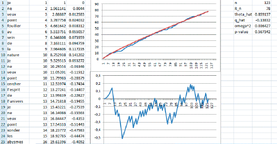
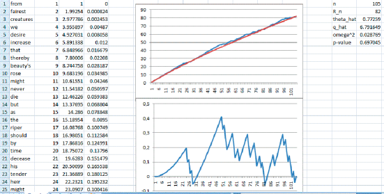
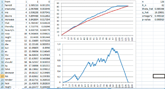
There is an example of French poetry, Les Regrets by Joachim du Bellay (1558), sonnet 1 (Fig. 1) and Shakespeare’s sonnet 1 (Fig. 2).

Figure 1: Les Regrets by Joachim du Bellay (1558), sonnet 1

All results for Shakespeare’s sonnets are in Appendix 3. Estimates of $\theta$ are restricted by 0.95.

Figure 2: Shakespeare’s sonnet 1

This approach can work with texts on any language.

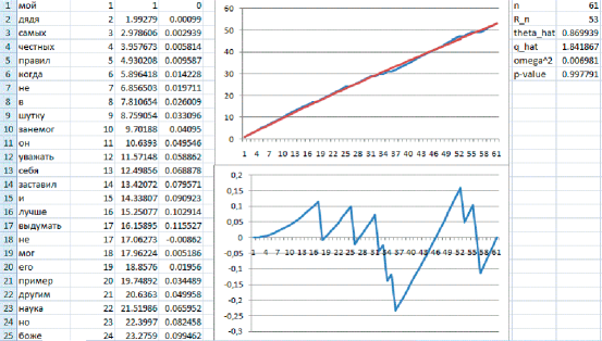
The first stanza of the first chapter of Eugene Onegin by Pushkin (Fig. 3).

Figure 3: The first stanza of the first chapter of Eugene Onegin by Pushkin

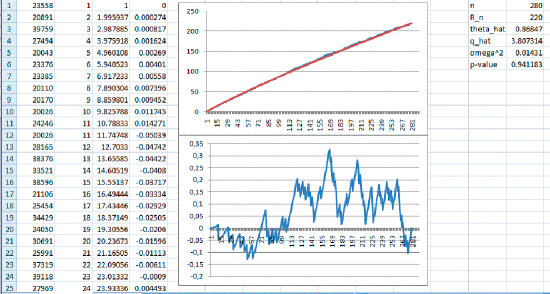
We used hieroglyphs instead of words when analyzing Chinese texts. On the first stage, we substituted hieroglyphs by their html codes. Danqing Painting by Du Fu (Fig. 4).

Figure 4: Danqing Painting by Du Fu

An example of a nonhomogeneous text is Shakespeare’s sonnet 1 with 3 repeated lines (Fig. 5).

Figure 5: Shakespeare’s sonnet 1 with 3 repeated lines

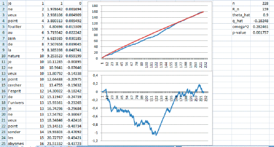
Another example of nonhomogeneity is a text from different languages. The example is Du Bellay’s sonnet 1 + Shakespeare’s sonnet 1 (Fig. 6).

Figure 6: Du Bellay’s sonnet 1 + Shakespeare’s sonnet 1

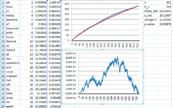
To have nonhomogeneity for a text in one language we need more long texts. Here the first three stanzas of Childe Harold’s Pilgrimage by Byron and the first three Shakespeare’s sonnets (Fig. 7).

Figure 7: The first three stanzas of Childe Harold’s Pilgrimage by Byron and the first three Shakespeare’s sonnets

5 Discussion

There are some open questions in the application of this approach. The first open question is Poisson approximation. If the number of identical words is small, then the Gaussian approximation is inaccurate. Barbour (2009) proposed an approximation by a translated Poisson distribution. We need a functional version of his theorem.

Another open question is the implementation of Simon model. Let $R_{n,1}$ be the number of words that occur exactly once. Under the assumptions made, there should be convergence $R_{n,1}/R_{n}\to\theta$ a.s. (Karlin, 1967). But real texts behave differently. Typically, the number of words that occur once is significantly less than $\widehat{\theta}R_{n}$.

Simon (1955) proposed the next stochastic model: the $(n+1)$-th word in the text is new with probability $p$; it coincides with each of the previous words with probability $(1-p)/n$. The drawback of Simon’s model is that the number of different words grows linearly. We need some kind of hybrid of an infinite urn model and Simon’s model.

Appendix 1. Proof of Theorem 2.3

Remember that

$$\widehat{\theta}=log_{2}^{+}(R_{n}/R_{n/2}),$$

$$r(k)=\sum_{i=1}^{\infty}(1-(1-\widehat{p}_{i})^{k}),$$

$$\widehat{p}_{i}=\widehat{c}(i+\widehat{q})^{-1/\widehat{\theta}}.$$

From Lemma 1 in Gnedin et al. (2007) we have

$$|{\bf E}R_{n}-{\bf E}R_{\Pi(n)}|<\frac{2}{n}{\bf E}R_{n,2}\leq\frac{2}{n}\times\frac{n}{2}=1.$$

Karlin (1967) proposed representation

$${\bf E}R_{\Pi(t)}=\int_{0}^{\infty}\alpha(ty)\frac{1}{y^{2}}e^{-1/y}dy,$$

$$\alpha(x)=\max\{j|p_{j}\geq\frac{1}{x}\}.$$

In our case

$$\alpha(x)=[(cx)^{\theta}-q].$$

We represent

$$\Gamma(k-\gamma)=\int_{0}^{\infty}y^{\gamma-k-1}e^{-1/y}dy.$$

So

$$(ct)^{\theta}\Gamma(1-\theta)-q-1\leq{\bf E}R_{\Pi(n)}\leq(ct)^{\theta}\Gamma(1-\theta)-q,$$

$${\bf E}R_{n}=(ct)^{\theta}\Gamma(1-\theta)-q+T_{n},\ \ |T_{n}|<2,$$

$$|r(n)-(\widehat{c}t)^{\widehat{\theta}}\Gamma(1-\widehat{\theta})+\widehat{q}|<2\ {\rm a.s.}$$

Now we estimate

$$\max_{1\leq k\leq n}\frac{|(k/n)^{\widehat{\theta}}R_{n}-r(k)|}{\sqrt{R_{n}}}.$$

We have

$$|(k/n)^{\widehat{\theta}}R_{n}-r(k)|=|(k/n)^{\widehat{\theta}}r(n)-r(k)|$$

$$<|(k/n)^{\widehat{\theta}}((\widehat{c}n)^{\widehat{\theta}}\Gamma(1-\widehat{\theta})-\widehat{q})-(\widehat{c}k)^{\widehat{\theta}}\Gamma(1-\widehat{\theta})+\widehat{q}|+4$$

$$=|\widehat{q}(1-(k/n)^{\widehat{\theta}})|+4\leq\widehat{q}+4.$$

As $R_{n}\to\infty$ a.s., it is enough to prove consistency of $\widehat{q}$ to have

$$\max_{1\leq k\leq n}\frac{|(k/n)^{\widehat{\theta}}R_{n}-r(k)|}{\sqrt{R_{n}}}\to 0$$

in probability.

Appendix 2. Calculation of $q_{ij}$

We calculate

$$q_{ij}=\int_{0}^{1}\int_{0}^{1}\widehat{K}(s,t)\sin\pi is\sin\pi jt\,dsdt.$$

We know $K(s,t)=(s+t)^{\theta}-\max(s^{\theta},t^{\theta})$,

$$\widehat{K}(s,t)=K(s,t)-s^{\theta}K(1,t)-t^{\theta}K(s,1)+s^{\theta}t^{\theta}K(1,1)$$

$$-t^{\theta}\log t\frac{K(s,1)-2^{\theta}K(s,1/2)}{\log 2}-s^{\theta}\log s\frac{K(t,1)-2^{\theta}K(t,1/2)}{\log 2}$$

$$+s^{\theta}t^{\theta}(\log s+\log t)\frac{K(1,1)-2^{\theta}K(1,1/2)}{\log 2}$$

$$+s^{\theta}t^{\theta}\log s\log t\frac{K(1,1)-2^{\theta+1}K(1,1/2)+2^{2\theta}K(1/2,1/2)}{\log^{2}2}.$$

Let us denote

$$J_{ij}=\int_{0}^{1}\int_{0}^{1}(s+t)^{\theta}\sin\pi is\sin\pi jt\,dsdt,$$

$$a(\theta,k,x)=\int_{0}^{x}t^{\theta}\sin\pi kt\,dt,\ \ b(\theta,k,x)=\int_{0}^{x}t^{\theta}\cos\pi kt\,dt,$$

$$A_{i}=\int_{0}^{1}t^{\theta}\sin\pi it\,dt=a(\theta,i,1),\ \ B_{i}=\int_{1}^{2}t^{\theta}\sin\pi it\,dt=a(\theta,i,2)-a(\theta,i,1),$$

$$C_{i}=\int_{0}^{1}t^{\theta+1}\cos\pi it\,dt=b(\theta+1,i,1),$$

$$D_{i}=\int_{1}^{2}t^{\theta}(2-t)\cos\pi it\,dt=2b(\theta,i,2)-2b(\theta,i,1)-b(\theta+1,i,2)+b(\theta+1,i,1),$$

$$E_{ij}=\int_{0}^{1}t^{\theta}\sin\pi it\cos\pi jt\,dt,\ \ F_{i}=\int_{0}^{1}K(t,1)\sin\pi it\,dt,$$

$$G_{i}=\int_{0}^{1}t^{\theta}\log t\sin\pi it\,dt,\ \ H_{i}=\int_{0}^{1}K(t,1/2)\sin\pi it\,dt.$$

Then we have

$$q_{ij}=J_{ij}-\frac{1}{\pi j}(A_{i}-E_{ij})-\frac{1}{\pi i}(A_{j}-E_{ji})$$

$$-A_{i}F_{j}-A_{j}F_{i}+K(1,1)A_{i}A_{j}$$

$$-G_{j}\frac{F_{i}-2^{\theta}H_{i}}{\log 2}-G_{i}\frac{F_{j}-2^{\theta}H_{j}}{\log 2}$$

$$+(A_{i}G_{j}+A_{j}G_{i})\frac{K(1,1)-2^{\theta}K(1,1/2)}{\log 2}$$

$$+G_{i}G_{j}\frac{K(1,1)-2^{\theta+1}K(1,1/2)+2^{2\theta}K(1/2,1/2)}{\log^{2}2}.$$

We calculate $J_{ij}$ substituting $t=u-s$, $s\leq u\leq s+1$. So

$$J_{ij}=\int_{0}^{1}u^{\theta}\,du\int_{0}^{u}\sin\pi is\sin\pi j(u-s)\,ds+\int_{1}^{2}u^{\theta}\,du\int_{u-1}^{1}\sin\pi is\sin\pi j(u-s)\,ds.$$

If $i\neq j$ then we have

$$J_{ij}=\frac{1}{2}\int_{0}^{1}u^{\theta}\,du\int_{0}^{u}(\cos\pi(is-ju+js)-\cos\pi(is+ju-js))\,ds$$

$$+\frac{1}{2}\int_{1}^{2}u^{\theta}\,du\int_{u-1}^{1}(\cos\pi(is-ju+js)-\cos\pi(is+ju-js))\,ds$$

$$=\frac{1}{2}\int_{0}^{1}u^{\theta}\left(\frac{\sin\pi iu+\sin\pi ju}{\pi(i+j)}-\frac{\sin\pi iu-\sin\pi ju}{\pi(i-j)}\right)\,du$$

$$+\frac{1}{2}\int_{1}^{2}u^{\theta}\left(\frac{\sin(\pi(i+j)-\pi ju)+\sin(\pi(i+j)-\pi iu)}{\pi(i+j)}-\frac{\sin(\pi(i-j)+\pi ju)+\sin(\pi(i-j)-\pi iu)}{\pi(i-j)}\right)\,du$$

$$=\frac{iA_{j}-jA_{i}-(-1)^{i+j}(iB_{j}-jB_{i})}{\pi(i^{2}-j^{2})}.$$

If $i=j$ then we have

$$J_{ii}=\frac{1}{2}\int_{0}^{1}u^{\theta}\,du\int_{0}^{u}(\cos\pi(2is-iu)-\cos\pi iu)\,ds+\frac{1}{2}\int_{1}^{2}u^{\theta}\,du\int_{u-1}^{1}(\cos\pi(2is-iu)-\cos\pi iu)\,ds$$

$$=\frac{1}{2}\int_{0}^{1}\left(u^{\theta}\frac{\sin\pi iu}{\pi i}-u^{\theta+1}\cos\pi iu\right)\,du$$

$$+\frac{1}{2}\int_{1}^{2}u^{\theta}\frac{\sin(2\pi i-\pi iu)-\sin(2\pi iu-2\pi i-\pi iu)}{2\pi i}\,du-\frac{1}{2}\int_{1}^{2}u^{\theta}(2-u)\cos\pi iu\,du$$

$$=\frac{A_{i}-B_{i}}{2\pi i}-\frac{C_{i}+D_{i}}{2}.$$

We know

$$a(\theta,k,x)=\pi kx^{\theta+2}\,{{}_{1}F_{2}}\left(\theta/2+1,3/2,\theta/2+2,-k^{2}\pi^{2}x^{2}/4\right)/(\theta+2),$$

$$b(\theta,k,x)=x^{\theta+1}\,{{}_{1}F_{2}}\left(\theta/2+1/2,1/2,\theta/2+3/2,-k^{2}\pi^{2}x^{2}/4\right)/(\theta+1),$$

$$E_{ij}=\frac{1}{2}A_{i+j}+\frac{1}{2}A_{i-j},$$

$$F_{i}=(-1)^{i}B_{i}+\frac{(-1)^{i}-1}{\pi i},$$

$$G_{i}=\int_{0}^{1}t^{\theta}\log t\sum_{k=0}^{\infty}\frac{(-1)^{k}(\pi it)^{2k+1}}{(2k+1)!}\,dt=-\sum_{k=0}^{\infty}\frac{(-1)^{k}(\pi i)^{2k+1}}{(2k+1)!(2k+\theta+2)^{2}}$$

$$=-{\pi i}\,{{}_{2}F_{3}}\left(\theta/2+1,\theta/2+1,3/2,\theta/2+2,\theta/2+2,-i^{2}\pi^{2}/4\right)/(\theta+2)^{2},$$

$$H_{i}=\int_{1/2}^{3/2}t^{\theta}\sin(\pi it-\pi i/2)\,dt+(\cos(\pi i/2)-1)2^{-\theta}/(\pi i)-\int_{1/2}^{1}t^{\theta}\sin\pi it\,dt$$

$$=\pi i\cos(\pi i/2)\bigg{(}(3/2)^{\theta+2}{{}_{1}F_{2}}\left(\theta/2+1,3/2,\theta/2+2,-9i^{2}\pi^{2}/16\right)$$

$$-2^{-\theta-2}{{}_{1}F_{2}}\left(\theta/2+1,3/2,\theta/2+2,-i^{2}\pi^{2}/16\right)\bigg{)}/(\theta+2)$$

$$-\sin(\pi i/2)\bigg{(}(3/2)^{\theta+1}{{}_{1}F_{2}}\left(\theta/2+1/2,1/2,\theta/2+3/2,-9i^{2}\pi^{2}/16\right)$$

$$-2^{-\theta-1}{{}_{1}F_{2}}\left(\theta/2+1/2,1/2,\theta/2+3/2,-i^{2}\pi^{2}/16\right)\bigg{)}/(\theta+1)$$

$$+(\cos(\pi i/2)-1)2^{-\theta}/(\pi i)-A_{i}+\pi i2^{-\theta-2}{{}_{1}F_{2}}\left(\theta/2+1,3/2,\theta/2+2,-i^{2}\pi^{2}/16\right)/(\theta+2).$$

${}_{1}F_{2}$ and ${}_{2}F_{3}$ are generalized hypergeometric functions, hyp1f2 and hyp2f3 in Python.

Appendix 3. Shakespeare’s sonnets

Sonnet No.	$n$	$R_{n}$	$\widehat{\theta}$	$\widehat{q}$	$\omega^{2}$	p-value
I	98	77	0.7911	5.1473	0.03139	0.6646
II	106	82	0.7877	5.2669	0.04696	0.4492
III	106	75	0.7859	2.9632	0.01184	0.9769
IV	96	74	0.8344	2.0164	0.02212	0.8257
V	96	80	0.9469	-0.5618	0.01114	0.9824
VI	100	70	0.7030	7.4855	0.03214	0.6579
VII	92	72	0.9031	-0.0988	0.00808	0.9970
VIII	101	78	0.8931	0.0952	0.01886	0.8818
IX	110	82	0.7877	4.2580	0.02714	0.7374
X	106	75	0.8890	-0.2561	0.00732	0.9985
XI	107	81	0.8804	0.3084	0.05376	0.3641
XII	109	81	0.9136	-0.4344	0.03236	0.6379
XIII	100	72	0.9031	-0.4163	0.01530	0.9375
XIV	106	78	0.8097	2.5711	0.02065	0.8525
XV	104	79	0.8280	2.2487	0.03427	0.6150
XVI	101	80	0.8301	3.0005	0.02032	0.8580
XVII	115	89	0.8319	2.7590	0.04821	0.4288
XVIII	107	79	0.8119	2.5560	0.02585	0.7592
XIX	106	83	0.9500	-0.7264	0.02625	0.7437
XX	106	85	0.8858	0.7206	0.00733	0.9984
XXI	109	78	0.8260	1.4855	0.01187	0.9768
XXII	112	74	0.7665	2.8193	0.02753	0.7315
XXIII	105	77	0.8074	2.5866	0.05756	0.3420
XXIV	112	78	0.7776	3.2625	0.02204	0.8286
XXV	101	78	0.8591	1.1303	0.01408	0.9537
XXVI	111	76	0.8217	1.1439	0.04744	0.4388
XXVII	103	77	0.8405	1.4188	0.03409	0.6166
XXVIII	109	75	0.8713	-0.0671	0.01646	0.9210
XXIX	107	79	0.9462	-0.7709	0.01810	0.8933
XXX	109	81	0.7549	6.4163	0.02698	0.7415
XXXI	108	73	0.6200	14.3674	0.14907	0.0698
XXXII	104	80	0.9125	-0.3063	0.03731	0.5592
XXXIII	103	82	0.8981	0.2218	0.00551	0.9998
XXXIV	112	86	0.8564	1.3410	0.01778	0.9004
XXXV	99	74	0.8171	2.3136	0.01207	0.9750
XXXVI	107	76	0.7561	4.7499	0.07452	0.2364
XXXVII	107	74	0.7500	4.4181	0.04462	0.4813
XXXVIII	103	83	0.8205	4.2305	0.01956	0.8713
XXXIX	111	77	0.8405	0.7001	0.02212	0.8255
XL	111	80	0.9500	-0.8142	0.21140	0.0068

Sonnet No.	$n$	$R_{n}$	$\widehat{\theta}$	$\widehat{q}$	$\omega^{2}$	p-value
XLI	102	72	0.7949	2.3792	0.06757	0.2699
XLII	120	71	0.7235	3.2051	0.04893	0.4369
XLIII	114	69	0.5850	13.1416	0.14373	0.0823
XLIV	110	83	0.8359	1.9066	0.01353	0.9602
XLV	98	78	0.9500	-0.7064	0.01251	0.9706
XLVI	107	67	0.8182	0.4581	0.05119	0.3994
XLVII	113	68	0.8021	0.6272	0.02254	0.8192
XLVIII	111	83	0.8515	1.1455	0.01952	0.8713
XLIX	104	74	0.8001	2.3442	0.01550	0.9353
L	110	83	0.8359	1.9066	0.01981	0.8667
LI	108	80	0.8301	1.8074	0.03863	0.5495
LII	102	76	0.8050	2.9384	0.00851	0.9958
LIII	99	62	0.7063	4.2012	0.03664	0.5900
LIV	103	77	0.7749	4.8369	0.01686	0.9156
LV	99	74	0.7832	4.1136	0.04431	0.4807
LVI	105	80	0.8625	0.8972	0.01015	0.9890
LVII	110	79	0.8944	-0.2682	0.01576	0.9311
LVIII	103	70	0.8439	0.3739	0.01275	0.9685
LIX	101	78	0.8260	2.6102	0.01904	0.8801
LX	100	79	0.7960	5.1082	0.01822	0.8941
LXI	114	78	0.8097	1.6042	0.01677	0.9168
LXII	98	66	0.8946	-0.4938	0.01837	0.8899
LXIII	103	78	0.7618	6.2212	0.02466	0.7823
LXIV	104	74	0.9241	-0.6534	0.06417	0.2700
LXV	106	85	0.9337	-0.4770	0.01424	0.9511
LXVI	82	65	0.8524	1.3890	0.00781	0.9976
LXVII	100	74	0.9241	-0.5877	0.01644	0.9204
LXVIII	99	75	0.9500	-0.7739	0.02632	0.7423
LXIX	114	81	0.8480	0.7358	0.01090	0.9843
LXX	102	75	0.8890	-0.1060	0.01452	0.9481
LXXI	115	76	0.7885	1.9740	0.01484	0.9442
LXXII	110	75	0.7370	4.9806	0.03965	0.5455
LXXIII	112	77	0.7590	3.9825	0.01696	0.9140
LXXIV	106	67	0.6738	6.6998	0.10606	0.1348
LXXV	109	77	0.8074	2.0411	0.02854	0.7118
LXXVI	107	72	0.6464	11.2969	0.10129	0.1534
LXXVII	101	70	0.9500	-0.8438	0.02176	0.8277
LXXVIII	102	74	0.7665	4.4436	0.07051	0.2570
LXXIX	108	74	0.7500	4.2387	0.03531	0.6059
LXXX	108	81	0.8641	0.7063	0.01128	0.9815

Sonnet No.	$n$	$R_{n}$	$\widehat{\theta}$	$\widehat{q}$	$\omega^{2}$	p-value
LXXXI	107	77	0.8074	2.2956	0.00920	0.9934
LXXXII	99	79	0.9115	-0.1166	0.01598	0.9276
LXXXIII	108	79	0.8775	0.1367	0.01685	0.9150
LXXXIV	106	77	0.8074	2.4361	0.01776	0.9015
LXXXV	103	80	0.7370	9.6313	0.04676	0.4585
LXXXVI	101	80	0.8957	0.2286	0.01423	0.9517
LXXXVII	110	81	0.9305	-0.6463	0.02146	0.8340
LXXXVIII	103	74	0.7176	7.5928	0.07136	0.2616
LXXXIX	104	79	0.8280	2.2487	0.03930	0.5403
XC	111	74	0.7176	5.6453	0.02559	0.7669
XCI	107	76	0.9500	-0.8264	0.09217	0.1262
XCI	112	74	0.7337	4.4914	0.03364	0.6326
XCIII	107	79	0.8443	1.1796	0.01119	0.9822
XCIV	96	74	0.9500	-0.7554	0.03898	0.5299
XCV	104	82	0.9500	-0.7170	0.04642	0.4318
XCVI	111	82	0.8657	0.5435	0.02981	0.6856
XCVII	100	84	0.9166	0.1683	0.00588	0.9997
XCVIII	110	79	0.7960	2.8866	0.01799	0.8978
XCIX	115	81	0.7853	3.1985	0.02053	0.8551
C	101	78	0.9279	-0.5258	0.00548	0.9998
CI	106	77	0.7590	5.1635	0.01166	0.9782
CII	108	79	0.8443	1.0814	0.00717	0.9987
CIII	108	74	0.6095	16.4318	0.21617	0.0247
CIV	107	85	0.9500	-0.7013	0.01698	0.9115
CV	98	62	0.6874	5.3704	0.02029	0.8592
CVI	103	75	0.9069	-0.4228	0.02428	0.7829
CVII	104	83	0.8672	1.3581	0.00865	0.9955
CVIII	106	85	0.9016	0.2122	0.02197	0.8261
CIX	108	72	0.7776	2.3672	0.01819	0.8947
CX	110	84	0.8225	2.8207	0.01456	0.9479
CXI	103	76	0.7885	3.6411	0.02730	0.7344
CXII	109	69	0.7510	2.7209	0.03853	0.5594
CXIII	110	74	0.7665	3.0736	0.03382	0.6274
CXIV	106	75	0.6897	9.5564	0.10235	0.1416
CXV	105	83	0.7026	15.1808	0.09517	0.1605
CXVI	103	78	0.8260	2.2610	0.01148	0.9800
CXVII	103	73	0.9044	-0.4676	0.02718	0.7296
CXVIII	105	80	0.8625	0.8972	0.03203	0.6482
CXIX	106	77	0.8238	1.7197	0.05184	0.3919
CXX	108	76	0.8050	2.0566	0.02387	0.7950

Sonnet No.	$n$	$R_{n}$	$\widehat{\theta}$	$\widehat{q}$	$\omega^{2}$	p-value
CXXI	107	79	0.7188	9.0289	0.03333	0.6383
CXXII	100	80	0.8141	4.2738	0.02785	0.7235
CXXIII	109	80	0.8301	1.6843	0.01845	0.8899
CXXIV	102	76	0.8729	0.3330	0.01468	0.9461
CXXV	100	83	0.8672	2.0726	0.00523	0.9999
CXXVI	88	68	0.8207	2.4595	0.02146	0.8380
CXXVII	102	79	0.8608	1.1231	0.02098	0.8454
CXXVIII	104	80	0.8790	0.4621	0.03259	0.6373
CXXIX	102	71	0.7574	3.9305	0.02730	0.7358
CXXX	114	81	0.8641	0.2990	0.00732	0.9985
CXXXI	111	73	0.7636	2.8441	0.03039	0.6829
CXXXII	107	80	0.7984	3.5647	0.01857	0.8884
CXXXIII	112	73	0.6820	7.4823	0.03948	0.5530
CXXXIV	112	71	0.8099	0.7968	0.05417	0.3717
CXXXV	108	71	0.7068	5.7796	0.11681	0.1039
CXXXVI	114	68	0.5956	11.5040	0.13579	0.0915
CXXXVII	115	81	0.8480	0.6669	0.00795	0.9973
CXXXVIII	109	74	0.7832	2.4423	0.01640	0.9224
CXXXIX	113	82	0.9500	-0.8080	0.02000	0.8600
CXL	111	84	0.7776	5.4863	0.01730	0.9088
CXLI	110	81	0.8007	3.1756	0.01889	0.8830
CXLII	109	74	0.7176	6.0534	0.02093	0.8485
CXLIII	112	78	0.7155	7.2400	0.04597	0.4701
CXLIV	105	74	0.8171	1.5352	0.00950	0.9922
CXLV	89	70	0.8439	1.7819	0.01051	0.9869
CXLVI	105	76	0.8217	1.7322	0.01653	0.9205
CXLVII	100	72	0.7949	2.6716	0.01535	0.9375
CXLVIII	116	77	0.8745	-0.2326	0.05124	0.3900
CXLIX	110	72	0.9220	-0.7360	0.02077	0.8471
CL	112	72	0.7437	3.4057	0.06262	0.3135
CLI	110	82	0.7877	4.2580	0.03491	0.6088
CLII	115	70	0.7030	4.5331	0.03797	0.5716
CLIII	102	75	0.8194	2.0017	0.06991	0.2506
CLIV	100	74	0.7500	6.0394	0.03911	0.5516

Acknowledgements

The research was supported by RFBR grant 19-51-53010. The authors like to thank Sergey Foss for helpful and constructive comments and suggestions.

Bahadur, R. R., 1960. On the number of distinct values in a large sample from an infinite discrete distribution. Proceedings of the National Institute of Sciences of India, 26A, Supp. II, 67–75.

Barbour, A. D., 2009. Univariate approximations in the infinite occupancy scheme. Alea 6, 415–433.

Barbour, A. D., Gnedin, A. V., 2009. Small counts in the infinite occupancy scheme. Electronic Journal of Probability, Vol. 14, Paper no. 13, 365–384.

Ben-Hamou, A., Boucheron, S., Ohannessian, M. I., 2017. Concentration inequalities in the infinite urn scheme for occupancy counts and the missing mass, with applications, Bernoulli, V. 23, No. 1, 249–287.

Chebunin, M., Kovalevskii, A., 2016. Functional central limit theorems for certain statistics in an infinite urn scheme. Statistics and Probability Letters, V. 119, 344–348.

Chebunin, M. G., Kovalevskii, A. P., 2019a. A statistical test for the Zipf’s law by deviations from the Heaps’ law, Siberian Electronic Mathematical Reports, V. 16, 1822–1832.

Chebunin, M., Kovalevskii, A., 2019b. Asymptotically Normal Estimators for Zipf’s Law, Sankhya A, V. 81, 482–492.

Decrouez, G., Grabchak, M., Paris, Q., 2018. Finite sample properties of the mean occupancy counts and probabilities, Bernoulli, V. 24, No. 3, 1910–1941.

Durieu, O., Wang, Y., 2016. From infinite urn schemes to decompositions of self-similar Gaussian processes, Electron. J. Probab., V. 21, paper No. 43, 23 pp.

Durieu, O., Samorodnitsky, G., Wang, Y., 2019. From infinite urn schemes to self-similar stable processes, Stochastic Processes and their Applications (in press).

Dutko, M., 1989. Central limit theorems for infinite urn models, Ann. Probab. 17, 1255–1263.

Eliazar, I., 2011. The Growth Statistics of Zipfian Ensembles: Beyond Heaps’ Law, Physica (Amsterdam) 390, 3189.

Gerlach, M., and Altmann, E. G., 2013. Stochastic Model for the Vocabulary Growth in Natural Languages. Physical Review X 3, 021006.

Gnedin, A., Hansen, B., Pitman, J., 2007. Notes on the occupancy problem with infinitely many boxes: general asymptotics and power laws. Probability Surveys, Vol. 4, 146–171.

Heaps, H. S., 1978. Information Retrieval: Computational and Theoretical Aspects, Academic Press.

Herdan, G., 1960. Type-token mathematics, The Hague: Mouton.

Hwang, H.-K., Janson, S., 2008. Local Limit Theorems for Finite and Infinite Urn Models. The Annals of Probability, Vol. 36, No. 3, 992–1022.

van Leijenhorst, D. C., van der Weide, T. P., 2005. A Formal Derivation of Heaps’ Law, Information Sciences (NY) 170, 263.

Mandelbrot, B., 1965. Information Theory and Psycholinguistics. In: B.B. Wolman and E. Nagel. Scientific psychology. Basic Books.

Nicholls, P. T., 1987. Estimation of Zipf parameters. J. Am. Soc. Inf. Sci., V. 38, 443–445.

Petersen, A. M., Tenenbaum, J. N., Havlin, S., Stanley, H. E., Perc, M., 2012. Languages cool as they expand: Allometric scaling and the decreasing need for new words. Scientific Reports 2, Article No. 943.

Smirnov, N.V., 1937. On the omega-squared distribution, Mat. Sb. 2, 973–993 (in Russian).

Zakrevskaya, N., Kovalevskii, A., 2019. An omega-square statistics for analysis of correspondence of small texts to the Zipf—Mandelbrot law. In: Applied methods of statistical analysis. Statistical computation and simulation. Proceedings of the International Workshop, Novosibirsk, NSTU, 488–494.

Zipf, G. K., 1936. The Psycho-Biology of Language, Routledge, London, 1936.