Power-law nonlinearity with maximally uniform distribution criterion for improved neural network training in automatic speech recognition

Abstract

In this paper, we describe the Maximum Uniformity of Distribution (MUD) algorithm with the power-law nonlinearity. In this approach, we hypothesize that neural network training will become more stable if feature distribution is not too much skewed. We propose two different types of MUD approaches: power function-based MUD and histogram-based MUD. In these approaches, we first obtain the mel filterbank coefficients and apply nonlinearity functions for each filterbank channel. With the power function-based MUD, we apply a power-function based nonlinearity where power function coefficients are chosen to maximize the likelihood assuming that nonlinearity outputs follow the uniform distribution. With the histogram-based MUD, the empirical Cumulative Density Function (CDF) from the training database is employed to transform the original distribution into a uniform distribution. In MUD processing, we do not use any prior knowledge (e.g. logarithmic relation) about the energy of the incoming signal and the perceived intensity by a human. Experimental results using an end-to-end speech recognition system demonstrate that power-function based MUD shows better result than the conventional Mel Filterbank Cepstral Coefficients (MFCCs). On the LibriSpeech database, we could achieve 4.02 % WER on test-clean and 13.34 % WER on test-other without using any Language Models (LMs). The major contribution of this work is that we developed a new algorithm for designing the compressive nonlinearity in a data-driven way, which is much more flexible than the previous approaches and may be extended to other domains as well.

Index Terms: Deep-Neural Network Model, end-to-end speech recognition, feature distribution, nonlinearity function, power function

1 Introduction

After the breakthrough of deep learning technology [1, 2, 3, 4, 5, 6, 7, 8], speech recognition accuracy has improved dramatically. Recently, speech recognition systems are widely used not only in smart phones and Personal Computers (PCs) but also in standalone devices in far-field environments. Examples include voice assistant systems such as Amazon Alexa , Google Home [9, 10], and Samsung Bixby [11].

In the era of deep neural networks, it has been frequently observed that the amount and coverage of the training data seem to be one of the most important factors to obtain better speech recognition accuracy [12, 13]. However, it is very difficult to gather sufficient amount of transcribed data from various domains. To overcome this problem, data augmentation has been very popular these days [14, 15, 16, 17, 18]. Small Power Boosting (SPB) technique may be considered as a variation of data augmentation techniques [19]. These kinds of data augmentation techniques have significantly improved speech recognition accuracy for commercial products such as Google Home [9, 10, 20]. However, a still remaining question is what would be the best way to obtain features as inputs to the neural network.

Using the capabilities of neural networks, researchers have explored raw-waveform features [21] or complex Fast Fourier Transform (FFT) features [9, 10]. However, log-mel filterbank coefficients or Mel Filterbank Cepstral Coefficients (MFCCs) [22] still remains the dominant form as features of the automatic speech recognition systems [5, 23, 24, 25]. This is because the conventional features such as MFCC or log-mel filterbank coefficients requires less computation than the neural network-based features such as raw-waveform features [26] while showing comparable performance. In log-mel filterbank coefficients and MFCC, the log-nonlinearity is employed to represent the relationship between the perceived sound intensity by human and the filterbank energy [27]. In more recent features such as Power Normalized Cepstral Coefficients (PNCCs), the power-law nonlinearity with the power coefficient of $\frac{1}{15}$ is employed [28, 29]. In our previous study [30, 31] this power-law nonlinearity has been shown to be more robust against additive noise. Both the log-law nonlinearity and the power-law nonlinearity with this specific coefficient of $\frac{1}{15}$ were motivated by the rate-intensity relation of the human auditory system [27, 28].

In this paper, we take a completely different approach. Instead of trying to model the human auditory system directly, we try to find a nonlinearity function which maximizes the uniformity of distribution. We refer this approach to Maximum Uniformity of Distribution (MUD) approach. This approach is based on the assumption that even though neural networks have remarkable capabilities in classifying input features, training would be easier if feature distribution is not too much skewed and features are not too much concentrated in an extremely narrow interval. More specifically, we assume that if the distributions of features are difficult to learn, parameter convergence usually becomes more difficult due to the erratic surfaces of error functions. In this case, we might have hard time in fine-tuning learning rates and hyper parameters to obtain converged parameters. In this paper, “easier” training means that the neural network may be trained well without too much fine-tuning thanks to the well-behaved feature distribution and the error function surface. It has been known that the distribution of amplitudes [32] and filterbank energies [33] is very sharp and skewed. Thus, it is usually not possible to use mel filterbank energy as features without using any compressive nonlinearity. We proposed two different types of MUD approaches: power function-based MUD and histogram-based MUD. In these approaches, we first obtain the mel filterbank energy. With the power function-based MUD, we apply a power-function based nonlinearity where the power function coefficient is chosen to maximize the likelihood assuming that the nonlinearity output is the uniform distribution. With the histogram-based MUD, the empirical Cumulative Density Function (CDF) is obtained from the training database to transform the original distribution into a uniform distribution. In these two approaches, unlike our previous study [28, 27], we do not use any prior knowledge about the rate-intensity relationship which is the relation between the energy of the incoming signal and the perceived intensity by a human [27]. However, as will be discussed in Sec. 3, we may obtain surprisingly similar coefficients to those obtained from human auditory systems in a data-driven way. A major contribution of this work is that we developed a new algorithm for designing the compressive nonlinearity in a data-driven way, which is much more flexible than the previous approaches and may be extended to other domains as well. Experimental results with an end-to-end speech recognition system demonstrate that Power-function based MUD shows better result than the conventional Mel Filterbank Cepstral Coefficients (MFCCs) while Histogram-based MUD shows comparable results to the MFCC processing.

The rest of the paper is organized as follows: We develop the theory of maximizing the uniformity in Sec. 2. We describe the MUD nonlinearity estimation and the entire end-to-end speech recognition system in Sec. 3. Experimental results that demonstrates the effectiveness of the MUD processing is presented in Sec. 4. We conclude in Sec. 5.

2 Maximization of Distribution Uniformity

2.1 Power-function based maximization of distribution uniformity

Consider a random variable $\mathbf{X}$ whose range is a closed interval $I_{\mathbf{X}}=\left[x_{\text{min}},x_{\text{max}}\right]$. $x_{\text{min}}$ and $x_{\text{max}}$ are the minimum and maximum values of the random variable $\mathbf{X}$ respectively.

Our objective is to apply a nonlinearity $\sigma_{p}(\cdot)$ in the form of (1) to $X$ so that the transformed random variable $Y$ closely follows a uniform distribution:

$$\mathbf{Y}=\sigma_{p}\left(\mathbf{X}\right)=(X-x_{\text{min}})^{\alpha}.$$ (1)

We chose the power function as the nonlinearity, partly because it has been shown that this function is quite effective as a compressive nonlinearity in speech feature processing [28, 29, 30, 31]. We subtract $X$ by $x_{\text{min}}$, since this will simplify the maximum likelihood estimation of $\alpha$, which will be explained shortly. From (1), the range of $Y$ is given by $I_{\mathbf{Y}}=\left[0,\left(x_{\text{max}}-x_{\text{min}}\right)^{\alpha}\right]$. Thus, we expect $Y$ to follow the following uniform distribution:

$$\mathbf{Y}\sim\mathcal{U}(0,\left(x_{\text{max}}-x_{\text{min}}\right)^{\alpha}).$$ (2)

The PDF of $Y$ is given by:

$$p_{\mathbf{Y}}(y)=\begin{cases}\frac{1}{\left(x_{\text{max}}-x_{\text{min}}\right)^{\alpha}},&0\leq y\leq\left(x_{\text{max}}-x_{\text{min}}\right)^{\alpha}\\ 0,\qquad&\text{otherwise}.\end{cases}$$ (3)

Using the property of the PDFs of the transformed random variables [34], we obtain the PDF of the random variable $\mathbf{X}$ by:

$$p_{\mathbf{X}}(x) =p_{\mathbf{Y}}(y)\frac{dy}{dx}$$

$$=p_{\mathbf{Y}}(y)\left[\alpha\left(x-x_{\text{min}}\right)^{\alpha-1}\right]$$

$$=\begin{cases}\frac{\alpha\left(x-x_{\text{min}}\right)^{\alpha-1}}{\left(x_{\text{max}}-x_{\text{min}}\right)^{\alpha}},\qquad&x_{\text{min}}\leq x\leq x_{\text{max}}\\ 0,&\text{otherwise}.\end{cases}$$ (4)

Now, suppose that we have the following $N$ samples from the random variable $\mathbf{X}$:

$$X=\left\{x_{0},x_{1},\cdots,x_{N-1}\right\}.$$ (5)

Using (4), we obtain the $\alpha$ value which maximizes the data likelihood $p(X|\alpha)$. The log likelihood of the data $X$ assuming the PDF in (2) is given by:

$$\mathcal{L}\left(\alpha;X\right) =\sum_{i=0}^{N-1}\ln p_{\mathbf{X}}\left(x_{i}\right)$$

$$=\sum_{i=0}^{N-1}\ln\left[\frac{\alpha(x_{i}-x_{\text{min}})^{\alpha-1}}{\left(x_{\text{max}}-x_{\text{min}}\right)^{\alpha}}\right]$$

$$=N\ln(\alpha)+\left(\alpha-1\right)\sum_{i=0}^{N-1}\ln\left(x_{i}-x_{\text{min}}\right)$$

$$\qquad-N\alpha\ln\left(x_{\text{max}}-x_{\text{min}}\right).$$ (6)

In (7), the term $\ln\left(x_{i}-x_{\text{min}}\right)$ is not defined when $x_{i}=x_{\text{min}}$. Thus, we apply flooring as shown below:

$$\mathcal{L}\left(\alpha;X\right) =N\ln(\alpha)$$

$$\quad+\left(\alpha-1\right)\sum_{i=0}^{N-1}\ln\left(\max\left\{x_{i}-x_{\text{min}},\delta\right\}\right)$$

$$\quad-N\alpha\ln\left(x_{\text{max}}-x_{\text{min}}\right),$$ (7)

where $\delta$ is a flooring coefficient. We use $\delta=10^{-100}$ in our experiments. By differentiating $\mathcal{L}\left(\alpha|X\right)$ with respect to $\alpha$, we obtain $\hat{\alpha}$, which maximizes the likelihood as below:

$$\hat{\alpha}=\frac{1}{\ln\left(\max\left\{x_{i}-x_{\text{min}},\delta\right\}\right)-\frac{1}{N}\sum_{i=0}^{N-1}\ln\left(x_{i}-x_{\text{min}}\right)}.$$ (8)

2.2 Histogram-based maximization of distribution uniformity

Instead of using the power-function based parametric approach to maximize the uniformity of distribution, we may also consider the non-parametric approach. In this approach, we estimate the Cumulative Distribution Function (CDF) from the samples in (5). This CDF estimation is achieved by sorting the samples $x_{i}$ in (5) and performing interpolation. The relation between the original random variable $\mathbf{X}$ and the transformed random variable $\mathbf{Y}$ is given by the following equation:

$$\mathbf{Y}=\sigma_{np}(\mathbf{X})=F_{u}^{-1}\left(\hat{F}_{x}(\mathbf{X})\right)$$ (9)

where $F_{u}(\cdot)$ is the CDF of the uniform distribution. $\hat{F}_{x}(\mathbf{X})$ in (9) is the estimated CDF of $\mathbf{X}$ that is mentioned above. In the special case of the uniform distribution of $\mathcal{U}(0,1)$, the inverse of this CDF is given by $F_{u}^{-1}(x)=x,\;\;0\leq x\leq 1$. Under this assumption, the above equation (9) may be simplified to:

$$\mathbf{Y}=\sigma_{np}(\mathbf{X})=\hat{F}_{x}(\mathbf{X}).$$ (10)

3 End-to-End speech recognition with the maximization of feature distribution uniformity

Fig. 1: The structure of the entire end-to-end speech recognition system with MUD processing. The LSTMs in the encoder layers may be either bidirectional-LSTMs or unidirectional-LSTMs. The attention may be either the full attention or the MOnotonic CHunkwise Attention (MoCha) [35, 36].

In this section, we explain how to use the theories we developed in Sec. 2.1 and 2.2 to train an end-to-end speech recognition system. The entire block diagram of the system is shown in Fig. 1. We used two different attention structures: Bidirectional LSTMs with Full Attention (BFA) [37] and MOnotonic CHunkwise Attention (MoCha) [35]. Our MoCha implementation is described in very detail in our another paper [36].

We apply either the power function-based MUD nonlinearity in (1) or the histogram-based MUD nonlinearity to each mel filterbank energy as the first step as depicted in Fig. 1. The mel filterbank energy is defined by the following equation:

$$p[m,l] =\sum_{k=0}^{K/2}\left|X[m,e^{j\omega_{k}}]\right|^{2}M_{l}[\omega_{k}]$$ (11)

where $M_{l}[\omega_{k}]$ is the triangular mel response for the $l$-th filterbank channel, $m$ is the frame index, and $K$ is the Fast Fourier Transform (FFT) size. $\omega_{k}$ is the discrete-time frequency defined by $\omega_{k}=\frac{2\pi k}{K}\;\;0\leq k\leq K-1$. The input feature vector $\vec{x}[m]$ in Fig. 1 is therefore given by:

$$\vec{x}[m]=\left[p[m,0],\;p[m,1],\;\cdots,\;p[m,C-1]\right].$$ (12)

where $C$ is the number of mel filter bank channels. In our experiments, we used the value of $C=40$. For the power function-based MUD, we use (8) for each mel filterbank channels from the randomly selected 1,000 utterances from the training set. In order not to be affected by the silence portion, we removed non-speech portion using a simple energy-based Voice Activity Detector (VAD).

Fig. 2 shows the estimated $\hat{\alpha}$ using (8) for each mel filterbank channel. From this Fig. 2, we observe that $\hat{\alpha}$ values are surprisingly close to the power coefficient of $\frac{1}{15}$ which we obtained by modeling the rate-intensity curve using a human auditory system [27, 28]. For the histogram-based MUD, we also used the same randomly selected 1,000 utterances from the training set, applied a VAD, and constructed the empirical CDF to obtain the nonlinearity function in (9).

Fig. 3 shows the Probability Density Functions (PDFs) of the mel filterbank energy in (a), those of the nonlinearity output using the power-based MUD in (b), and those of the nonlinearity output using the histogram-based MUD in (c). In plotting these PDFs in Fig. 3, we used another 1,000 utterances which are not included in estimating the MUD nonlinearities. These plots are for the third filterbank channel $l=3$ in (11). As shown in Fig. 3b, if we use the power function-based MUD, the PDF becomes much smoother compared to the original PDF in Fig. 3a. However, this PDF is not as uniform as the one in Fig. 3c. In Fig. 4, we compared the Power-law nonlinearity of the form of $(\cdot)^{\frac{1}{15}}$ used in PNCC [28, 29], power function-based MUD in (1), and histogram-based MUD (9) for the third mel filterbank channel $l=3$ in (11). Note that in case of power function-based MUD and histogram-based MUD, the nonlinearity functions are different for different filterbank channels.

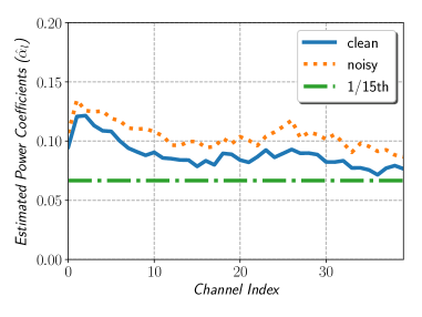
Fig. 2: The estimated power coefficients for each mel filterbank channels using (8).

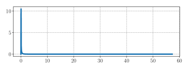
(a)

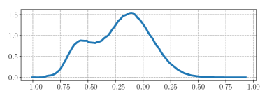
(b)

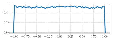
(c)

Fig. 3: The Probability Density Functions for the third filterbank channel of (a): the mel filterbank energy $p[m,l],l=3$ in (11), (b): the power-function based MUD output of this mel filterbank energy in (1), (c) the histogram based-MUD in (9).

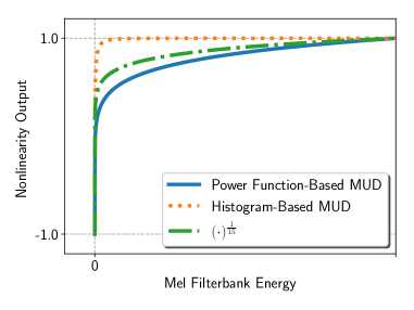
Fig. 4: Comparison of different nonlinearities: Power-law nonlinearity of the form of $(\cdot)^{\frac{1}{15}}$ used in PNCC [28, 29], power function-based MUD in (1), and histogram-based MUD (9) for the third mel filterbank channel.

Table 1: Word Error Rates (WERs) obtained with MFCC, Power Mel filterbank coefficients,
power function-based MUD processing, and histogram-based MUD Processing on the LibriSpeech corpus [38].
For each WER number, the same experiment was conducted twice and the results were averaged.
All these results were obtained without using a Language Model (LM).

Neural Network Structure		MFCC	$(\cdot)^{\frac{1}{15}}$	Power Function- Based MUD	Histogram- Based MUD
1024 cell ULSTM MoCha	test-clean	7.09 %	7.04 %	7.10 %	7.13 %
	test-other	20.60 %	19.76 %	19.64 %	20.03 %
	average	13.85 %	13.40 %	13.37 %	13.58 %
1536 cell BLSTM Full-Attention	test-clean	4.06 %	3.94 %	4.02 %	4.11 %
	test-other	13.97 %	13.56 %	13.34 %	14.10 %
	average	9.02 %	8.75 %	8.68 %	9.11 %

We used the RETURNN speech recognition system [39, 40, 41]. We have tried various modifications to the training stratgegy (e.g [42, 43]). $\vec{x}[n]$ and $\vec{y}_{l}$ are the input mel filterbank energy vector and the output label , respectively. $m$ is the input frame index and $l$ is the decoder output step index. $\vec{c}_{l}$ is the attention context vector calculated as a weighted sum of the encoder hidden state vectors $\vec{h}_{enc}[m]$. The weights used in this procedure is called the attention weights. They are calculated by applying softmax to the attention energies [37, 40]. $\vec{h}^{enc}[m]$ and $\vec{h}^{dec}_{l}$ are the encoder and the decoder hidden state vectors, respectively. $\vec{\beta}_{l}[m]$ is the attention weight feedback [40]. In [40], the peak value of the speech waveform is normalized to be one. However, since finding the peak sample value is not possible for on-line feature extraction, we did not perform this normalization. We modified the input pipeline so that the on-line feature generation can be performed. We disabled the clipping of feature range between -3 and 3, which is the default setting in their LibriSpeech experiment in [40]. We conducted experiments using both the uni-directional and bi-directional Long Short-Term Memories (LSTMs) [44]. For on-line processing, we used the MOnotonic CHunkwise Attention (MoCha) [35]. In online speech recognition experiments using MoCha, we used the chunk size of 2. For better stability in the LSTM training, we used the gradient clipping by global norm [45], which is implemented as tf.clip_by_global_norm API in Tensorflow [46]. We used six layers of encoders and one layer of decoder followed by a softmax layer. The training infrastructure we used is described in more detail in our another paper [47].

4 Experimental Results

For speech recognition experiments, we used the Librispeech database [38] for training and evaluation. For training, we used the entire 960 hours training set consisting of 281,241 utterances. For evaluation, we used the official 5.4 hours test-clean and 5.1 hours test-other databases. We conducted experiments using the 40-th order MFCC feature implemented in [48], power-law nonlinearity of $(\cdot)^{\frac{1}{15}}$ applied to the mel filterbank energy, power function based MUD processing, and histogram-based MUD processing. We conducted experiments using both the online ULSTM/MoCha [35] structure and the BLSTM with the full-attention structure. We have conducted Bidirectional Long Short-Term Memory (BLSTM) experiments with the cell size of 1536. For the on-line MoCha experiment, we used the Uni-directional Long Short-term Memory (ULSTM) with the cell size of 1024. Our MoCha implementation is described in very detail in [36]. In all of our experiments in this section, we did not use any external Language Models (LMs). We observed that external LMs can significantly enhance the speech recognition accuracy of our end-to-end speech recognition system, which is shown in our other papers [18, 47]. However, in this paper, just to focus on the effects of nonlinearity, we did not employ external LMs.

These results are summarized in Table 1. For each WER number in this table, the same experiment was conducted twice and these results were averaged to reduce the effect of random fluctuation in each trial. The best performance was achieved when we used the power function-based MUD with the 1536-cell BLSTM layers in the encoder and the full attention. For the test-clean and test test-other test sets [38] , we obtained 4.02 % Word Error Rate (WER) and 13.34 % WER, respectively. On average, the WER was 8.68 %, which is relatively 3.77 % improvement over the baseline MFCC with 9.02 % WER. From Table. 1, we note that usually there is no improvement over the baseline MFCC on the test-clean set. However, improvement on the test-other was usually more substantial. For the 1536-cell BLSTM full-attention case, the relative improvement over the baseline MFCC on the test-other is 4.51 %. The performance difference between the power-law nonlinearity of $(\cdot)^{\frac{1}{15}}$ and the power function-based MUD is usually very small. This was expected since the estimated parameters using (8) are not very different from $\frac{1}{15}$ as shown in Fig. 2. However, for the test-other database, which is more a difficult set, the improvement over the power-law nonlinearity of $(\cdot)^{\frac{1}{15}}$ is statistically significant. Histogram-based MUD shows somewhat worse performance compared to power function-based MUD. However, this histogram- based MUD still shows comparable results to the conventional MFCC processing. For the histogram-based MUD, we also tried to transform the PDF into a Gaussian distribution. However, that system showed slightly worse results than the Histogram-based MUD in Table 1. We hypothesize that the reason why histogram-based MUD does slightly worse than the power-function based MUD is that it somewhat obscured the energy boundary between speech vs non-speech. If we can employ a very sharp VAD to select only the speech portion very accurately, we think the performance of the histogram-based MUD will be comparable to that of the power-funcation based MUD.

5 Conclusions

In this paper, we described the Maximum Uniformity of Distribution (MUD) algorithm. This approach is based on the assumption that neural-network training would be easier and the converged parameters would show better performance when feature distribution is not too much skewed or too much concentrated in an extremely narrow interval. We proposed two different types of MUD approaches: power function-based MUD and histogram -based MUD. In these approaches, we first obtain the Mel filterbank coefficients. The estimated parameters using the power function-based MUD using (8) are surprisingly close to the power coefficient of $\frac{1}{15}$ which we obtained by modeling the rate-intensity curve using a human auditory system [27, 28]. The histogram-based MUD shows comparable performance to the conventional MFCC processing, but it was worse than the performacne of the power function-based MUD. In the end-to-end speech recognition experiments on the LibriSpeech databases [38], we obtained 4.02 % WER and 13.34 % WER on the test-clean and test test-other test sets respectively using the power function-based MUD processing.

The major novelty of this paper is that we proposed a new way of deriving a suitable nonlinearty from the training data themselves in a data-driven way. In the case of the previous power-law nonlinearty with the power coefficients of $\frac{1}{10}$ [31] or $\frac{1}{15}$ [29], they were obtained either by curve-fitting from the rate-intensity curve of the human auditory system [28] or by performing speech recognition experiments with various power coefficients to find out the optimal value [27]. Since these steps require significant amount time, we could not fine-tune the power coefficient for each filter bank channel in our previous work [28]. In this new MUD approach, we obtain suitable coefficients for each filterbank channel “without” actually running speech recognition experiments. This is a significant advantage compared to the previous hand-crafted fine-tuning. In addition, we believe that this approach is not only limited to speech recognition, but it can be applied to other domains in the future. Since the previous power coefficient of $\frac{1}{15}$ was already hand-optimized by performing experiments with different coefficients, it is quite natural that the additional improvement of MUD over the previous power-law nonlinearity is relatively small, which is also shown in Section 4. Nevertheless, the major contribution of this work is that we proposed a new way of designing the compressive nonlinearity in a data-driven way, and this approach is much more flexible and may be extended to other domains as well.

References

- [1] M. Seltzer, D. Yu, and Y.-Q. Wang, “An investigation of deep neural networks for noise robust speech recognition,” in Int. Conf. Acoust. Speech, and Signal Processing, 2013, pp. 7398–7402.
- [2] D. Yu, M. L. Seltzer, J. Li, J.-T. Huang, and F. Seide, “Feature learning in deep neural networks - studies on speech recognition tasks,” in Proceedings of the International Conference on Learning Representations, 2013.
- [3] V. Vanhoucke, A. Senior, and M. Z. Mao, “Improving the speed of neural networks on CPUs,” in Deep Learning and Unsupervised Feature Learning NIPS Workshop, 2011.
- [4] G. Hinton, L. Deng, D. Yu, G. E. Dahl, A. Mohamed, N. Jaitly, A. Senior, V. Vanhoucke, P. Nguyen, T. Sainath, and B. Kingsbury, “Deep neural networks for acoustic modeling in speech recognition: The shared views of four research groups,” IEEE Signal Processing Magazine, vol. 29, no. 6, Nov. 2012.
- [5] H. Hadian, H. Sameti, D. Povey, and S. Khudanpur, “End-to-end speech recognition using lattice-free mmi,” in Proc. Interspeech 2018, 2018, pp. 12–16. [Online]. Available: http://dx.doi.org/10.21437/Interspeech.2018-1423
- [6] S. Karita, N. E. Y. Soplin, S. Watanabe, M. Delcroix, A. Ogawa, and T. Nakatani, “Improving Transformer-Based End-to-End Speech Recognition with Connectionist Temporal Classification and Language Model Integration,” in Proc. Interspeech 2019, 2019, pp. 1408–1412. [Online]. Available: http://dx.doi.org/10.21437/Interspeech.2019-1938
- [7] C.-C. Chiu, T. N. Sainath, Y. Wu, R. Prabhavalkar, P. Nguyen, Z. Chen, A. Kannan, R. J. Weiss, K. Rao, E. Gonina, N. Jaitly, B. Li, J. Chorowski, and M. Bacchiani, “State-of-the-art speech recognition with sequence-to-sequence models,” in 2018 IEEE International Conference on Acoustics, Speech and Signal Processing (ICASSP), April 2018, pp. 4774–4778.
- [8] R. Prabhavalkar, K. Rao, T. N. Sainath, B. Li, L. Johnson, and N. Jaitly, “A comparison of sequence-to-sequence models for speech recognition,” in Proc. Interspeech 2017, 2017, pp. 939–943. [Online]. Available: http://dx.doi.org/10.21437/Interspeech.2017-233
- [9] C. Kim, A. Misra, K. Chin, T. Hughes, A. Narayanan, T. N. Sainath, and M. Bacchiani, “Generation of large-scale simulated utterances in virtual rooms to train deep-neural networks for far-field speech recognition in google home,” in Proc. Interspeech 2017, 2017, pp. 379–383. [Online]. Available: http://dx.doi.org/10.21437/Interspeech.2017-1510
- [10] B. Li, T. Sainath, A. Narayanan, J. Caroselli, M. Bacchiani, A. Misra, I. Shafran, H. Sak, G. Pundak, K. Chin, K-C Sim, R. Weiss, K. Wilson, E. Variani, C. Kim, O. Siohan, M. Weintraub, E. McDermott, R. Rose, and M. Shannon, “Acoustic modeling for Google Home,” in INTERSPEECH-2017, Aug. 2017, pp. 399–403.
- [11] “Samsung bixby,” http://www.samsung.com/bixby/.
- [12] H. Soltau, H. Liao, and H. Sak, “Neural speech recognizer: Acoustic-to-word lstm model for large vocabulary speech recognition,” in INTERSPEECH-2017, 2017, pp. 3707–3711. [Online]. Available: http://dx.doi.org/10.21437/Interspeech.2017-1566
- [13] A. Narayanan, A. Misra, K. C. Sim, G. Pundak, A. Tripathi, M. Elfeky, P. Haghani, T. Strohman, and M. Bacchiani, “Toward domain-invariant speech recognition via large scale training,” in 2018 IEEE Spoken Language Technology Workshop (SLT), Dec 2018, pp. 441–447.
- [14] W. Hartmann, T. Ng, R. Hsiao, S. Tsakalidis, and R. Schwartz, “Two-stage data augmentation for low-resourced speech recognition,” in INTERSPEECH-2016, 2016, pp. 2378–2382. [Online]. Available: http://dx.doi.org/10.21437/Interspeech.2016-1386
- [15] X. Cui, V. Goel, and B. Kingsbury, “Data augmentation for deep neural network acoustic modeling,” IEEE/ACM Transactions on Audio, Speech, and Language Processing, vol. 23, no. 9, pp. 1469–1477, Sept 2015.
- [16] D. S. Park, W. Chan, Y. Zhang, C.-C. Chiu, B. Zoph, E. D. Cubuk, and Q. V. Le, “SpecAugment: A Simple Data Augmentation Method for Automatic Speech Recognition,” in Proc. Interspeech 2019, 2019, pp. 2613–2617. [Online]. Available: http://dx.doi.org/10.21437/Interspeech.2019-2680
- [17] C. Kim, T. Sainath, A. Narayanan, A. Misra, R. Nongpiur, and M. Bacchiani, “Spectral distortion model for training phase-sensitive deep-neural networks for far-field speech recognition,” in 2018 IEEE International Conference on Acoustics, Speech and Signal Processing (ICASSP), April 2018, pp. 5729–5733.
- [18] C. Kim, M. Shin, A. Garg, and D. Gowda, “Improved Vocal Tract Length Perturbation for a State-of-the-Art End-to-End Speech Recognition System,” in INTERSPEECH-2019, Graz, Austria, Sept. 2019, pp. 739–743. [Online]. Available: http://dx.doi.org/10.21437/Interspeech.2019-3227
- [19] C. Kim, K. Kumar and R. M. Stern, “Robust speech recognition using small power boosting algorithm,” in IEEE Automatic Speech Recognition and Understanding Workshop, Dec. 2009, pp. 243–248.
- [20] C. Kim, E. Variani, A. Narayanan, and M. Bacchiani, “Efficient implementation of the room simulator for training deep neural network acoustic models,” in INTERSPEECH-2018, Sept 2018, pp. 3028–3032. [Online]. Available: http://dx.doi.org/10.21437/Interspeech.2018-2566
- [21] T. Sainath, R. J. Weiss, K. W. Wilson, B. Li, A. Narayanan, E. Variani, M. Bacchiani, I. Shafran, A. Senior, K. Chin, A. Misra, and C. Kim, “Multichannel signal processing with deep neural networks for automatic speech recognition,” IEEE/ACM Trans. Audio, Speech, Lang. Process., Feb. 2017.
- [22] P. Mermelstein, “Automatic segmentation of speech into syllabic units,” J. Acoust. Soc. of Am., vol. 58, pp. 880–883, Jan. 1975.
- [23] D. Amodei, S. Ananthanarayanan, R. Anubhai, J. Bai, E. Battenberg, C. Case, J. Casper, B. Catanzaro, Q. Cheng, G. Chen et al., “Deep speech 2 : End-to-end speech recognition in english and mandarin,” in Proceedings of The 33rd International Conference on Machine Learning, ser. Proceedings of Machine Learning Research, M. F. Balcan and K. Q. Weinberger, Eds., vol. 48. New York, New York, USA: PMLR, 20–22 Jun 2016, pp. 173–182. [Online]. Available: http://proceedings.mlr.press/v48/amodei16.html
- [24] C. Kim, A. Menon, M. Bacchiani, and R. Stern, “Sound source separation using phase difference and reliable mask selection selection,” in 2018 IEEE International Conference on Acoustics, Speech and Signal Processing (ICASSP), April 2018, pp. 5559–5563.
- [25] C. Kim, K. Chin, M. Bacchiani, and R. M. Stern, “Robust speech recognition using temporal masking and thresholding algorithma,” in INTERSPEECH-2014, Sept. 2014, pp. 2734–2738.
- [26] T. Sainath, R. Weiss, K. Wilson, A. Narayanan, and M. Bacchiani, “Learning the Speech Front-end With Raw Waveform CLDNNs,” in INTERSPEECH-2015, Sept. 2015, pp. 1–5.
- [27] C. Kim, “Signal processing for robust speech recognition motivated by auditory processing,” Ph.D. dissertation, Carnegie Mellon University, Pittsburgh, PA USA, Dec. 2010.
- [28] C. Kim and R. M. Stern, “Power-Normalized Cepstral Coefficients (PNCC) for Robust Speech Recognition,” IEEE/ACM Trans. Audio, Speech, Lang. Process., pp. 1315–1329, July 2016.
- [29] C. Kim and R. M. Stern, “Power-normalized cepstral coefficients (pncc) for robust speech recognition,” in IEEE Int. Conf. on Acoustics, Speech, and Signal Processing, March 2012, pp. 4101–4104.
- [30] ——, “Feature extraction for robust speech recognition based on maximizing the sharpness of the power distribution and on power flooring,” in IEEE Int. Conf. on Acoustics, Speech, and Signal Processing, March 2010, pp. 4574–4577.
- [31] ——, “Feature extraction for robust speech recognition using a power-law nonlinearity and power-bias subtraction,” in INTERSPEECH-2009, Sept. 2009, pp. 28–31.
- [32] ——, “Robust signal-to-noise ratio estimation based on waveform amplitude distribution analysis,” in INTERSPEECH-2008, Sept. 2008, pp. 2598–2601.
- [33] ——, “Power function-based power distribution normalization algorithm for robust speech recognition,” in IEEE Automatic Speech Recognition and Understanding Workshop, Dec. 2009, pp. 188–193.
- [34] A Papoulis and S. U. Pillai, Probability, Random Variables and Stochastic Processes. New York, NY: McGraw-Hill, 2002.
- [35] C.-C. Chiu and C. Raffel, “Monotonic chunkwise attention,” in International Conference on Learning Representations, Apr. 2018. [Online]. Available: https://openreview.net/forum?id=Hko85plCW
- [36] K. Kim, K. Lee, D. Gowda, J. Park, S. Kim, S. Jin, Y.-Y. Lee, J. Yeo, D. Kim, S. Jung, J. Lee, M. Han, and C. Kim, “attention based on-device streaming speech recognition with large speech corpus,” in 2019 IEEE Automatic Speech Recognition and Understanding Workshop (ASRU), Dec. 2019 (accepted).
- [37] D. Bahdanau, K. Cho, and Y. Bengio, “Neural machine translation by jointly learning to align and translate,” in 3rd International Conference on Learning Representations, ICLR 2015, San Diego, CA, USA, May 7-9, 2015, Conference Track Proceedings, 2015. [Online]. Available: http://arxiv.org/abs/1409.0473
- [38] V. Panayotov, G. Chen, D. Povey, and S. Khudanpur, “Librispeech: An asr corpus based on public domain audio books,” in IEEE Int. Conf. Acoust., Speech, and Signal Processing, April 2015, pp. 5206–5210.
- [39] P. Doetsch, A. Zeyer, P. Voigtlaender, I. Kulikov, R. Schlüter, and H. Ney, “RETURNN: the RWTH extensible training framework for universal recurrent neural networks,” in IEEE Int. Conf. Acoust., Speech, and Signal Processing, March 2017, pp. 5345–5349.
- [40] A. Zeyer, K. Irie, R. Schlüter, and H. Ney, “Improved training of end-to-end attention models for speech recognition,” in INTERSPEECH-2018, 2018, pp. 7–11. [Online]. Available: http://dx.doi.org/10.21437/Interspeech.2018-1616
- [41] C. Lüscher, E. Beck, K. Irie, M. Kitza, W. Michel, A. Zeyer, R. Schlüter, and H. Ney, “RWTH ASR Systems for LibriSpeech: Hybrid vs Attention,” in Proc. Interspeech 2019, 2019, pp. 231–235. [Online]. Available: http://dx.doi.org/10.21437/Interspeech.2019-1780
- [42] D. Gowda, A. Garg, K. Kim, M. Kumar, and C. Kim, “Multi-task multi-resolution char-to-bpe cross-attention decoder for end-to-end speech recognition,” in INTERSPEECH-2019, Graz, Austria, Sept. 2019, pp. 2783–2787. [Online]. Available: http://dx.doi.org/10.21437/Interspeech.2019-3216
- [43] A. Garg, D. Gowda, A. Kumar, K. Kim, M. Kumar, and C. Kim, “Improved multi-stage training of online attention-based encoder-decoder models,” in 2019 IEEE Automatic Speech Recognition and Understanding Workshop (ASRU), Dec. 2019 (accepted).
- [44] S. Hochreiter and J. Schmidhuber, “Long short-term memory,” Neural Computation, no. 9, pp. 1735–1780, Nov. 1997.
- [45] R. Pascanu, T. Mikolov, and Y. Bengio, “On the difficulty of training recurrent neural networks,” in Proceedings of the 30th International Conference on International Conference on Machine Learning - Volume 28, ser. ICML’13. JMLR.org, 2013, pp. III–1310–III–1318. [Online]. Available: http://dl.acm.org/citation.cfm?id=3042817.3043083
- [46] M. Abadi, P. Barham, J. Chen, Z. Chen, A. Davis, J. Dean, M. Devin, S. Ghemawat, G. Irving, M. Isard, M. Kudlur, J. Levenberg, R. Monga, S. Moore, D. G. Murray, B. Steiner, P. Tucker, V. Vasudevan, P. Warden, M. Wicke, Y. Yu, and X. Zheng, “Tensorflow: A system for large-scale machine learning,” in 12th USENIX Symposium on Operating Systems Design and Implementation (OSDI 16). Savannah, GA: USENIX Association, 2016, pp. 265–283. [Online]. Available: https://www.usenix.org/conference/osdi16/technical-sessions/presentation/abadi
- [47] C. Kim, S. Kim, K. Kim, M. Kumar, J. Kim, K. Lee, C. Han, A. Garg, E. Kim, M. Shin, S. Singh, L. Heck, and D. Gowda, “End-to-end training of a large vocabulary end-to-end speech recognition system,” in 2019 IEEE Automatic Speech Recognition and Understanding Workshop (ASRU), Dec. 2019 (accepted).
- [48] B. McFee, C. Raffel, D. Liang, D. P. Ellis, M. McVicar, E. Battenberg, and O. Nieto, “librosa: Audio and music signal analysis in python,” in Proceedings of the 14th Python in Science Conference, K. Huff and J. Bergstra, Eds., 2015, pp. 18 – 25.