End-to-end Training of a Large Vocabulary
End-to-end Speech Recognition System

Abstract

In this paper, we present an end-to-end training framework for building state-of-the-art end-to-end speech recognition systems. Our training system utilizes a cluster of Central Processing Units (CPUs) and Graphics Processing Units (GPUs). The entire data reading, large scale data augmentation, neural network parameter updates are all performed “on-the-fly”. We use vocal tract length perturbation [1] and an acoustic simulator [2] for data augmentation. The processed features and labels are sent to the GPU cluster. The Horovod allreduce approach is employed to train neural network parameters. We evaluated the effectiveness of our system on the standard Librispeech corpus [3] and the 10,000-hr anonymized Bixby English dataset. Our end-to-end speech recognition system built using this training infrastructure showed a 2.44 % WER on test-clean of the LibriSpeech test set after applying shallow fusion with a Transformer language model (LM). For the proprietary English Bixby open domain test set, we obtained a WER of 7.92 % using a Bidirectional Full Attention (BFA) end-to-end model after applying shallow fusion with an RNN-LM. When the monotonic chunckwise attention (MoCha) based approach is employed for streaming speech recognition, we obtained a WER of 9.95 % on the same Bixby open domain test set.

Index Terms: end-to-end speech recognition, distributed training, example server, data augmentation, acoustic simulation

1 Introduction

In recent years, deep learning techniques have significantly improved speech recognition accuracy [4, 5, 6, 7, 8]. This improvement has come about from the shift from Gaussian Mixture Model (GMM) to the Feed-Forward Deep Neural Networks (FF-DNNs), FF-DNNs to Recurrent Neural Network (RNN) and in particular the Long Short-Term Memory (LSTM) networks [9]. Thanks to these advances, voice assistant devices such as Google Home [2, 10] , Amazon Alexa or Samsung Bixby [11] are being used at many homes and on personal devices.

Recently there has been increasing interest in switching from the conventional Weighted Finite State Transducer (WFST) based decoder using an Acoustic Model (AM) and a Language Model (LM) to a complete end-to-end all-neural speech recognition systems [12, 13, 14]. These complete end-to-end systems have started surpassing the performance of the conventional WFST-based decoders with a very large training database [15], a better choice of target unit such as Byte Pair Encoded (BPE) subword units, and an improved training methodology such as Minimum Word Error Rate (MWER) training [16].

Another important aspect in building high-performance speech recognition systems is the amount and the coverage of the training data. To build high performance speech recognition systems for conversational speech, we need to use a large amount of speech data covering various domains [17]. In [18], it has been shown that we need a very large training set ($\sim$125,000 hours of semi-supervised speech data) to achieve high speech recognition accuracy for difficult tasks like video captioning. To train neural networks using such large amounts of speech data, we usually need multiple Central Processing Units (CPUs) or Graphics Processing Units (GPUs) [19, 20].

With widespread adoption of voice assistant speakers, far-field speech recognition has become very important. In far-field speech recognition, the impacts of reverberation and noise are much larger than those in near-field cases. Traditional approaches to far-field speech recognition include noise robust feature extraction algorithms [21, 22, 23], or multi-microphone approaches [24, 25, 26, 27, 28, 29, 30]. More recently, approaches using data augmentation has been gaining popularity for far-field speech recognition [31, 32, 33, 34, 35]. An “acoustic simulator” [2, 36] is used to generate simulated speech utterances for millions of different room dimensions, a wide distribution of reverberation time and signal-to-noise ratio. In a similar spirit, Vocal Tract Length Perturbation (VTLP) has been proposed [37] to tackle the speaker variability issue. As shown in our recent paper [1], VTLP is especially useful when the speaker variability in the training database is not sufficient. For these kinds of data augmentation, processing on CPUs is more desirable than processing on GPUs. Due to this, we have proposed an end-to-end training approach using Example Servers (ES) and workers. Example servers are typically run on the CPU cluster performing data reading, data augmentation, and feature extraction [19, 36].

Fig. 1: The Samsung Research end-to-end training framework for building an end-to-end speech recognition system with multi CPU-GPU clusters and on-the-fly data processing and augmentation pipeline.

In this paper, we describe the structure of our end-to-end training system to train an end-to-end speech recognition system. This training system has several advantages over previous systems described in [36]. First, instead of using the QueueRunner, we use a more efficient data queue using tf.data in Tensorflow [38]. Second, instead of pre-calculating information about room configurations and room impulse responses in the acoustic simulator, these are calculated on-the-fly. Thus, the entire training system runs on-the-fly. Additionally, instead of using the parameter server-worker structure, we use an allreduce approach implemented in the Horovod [39] distributed training framework, which has been shown to be more efficient. The system described in [19], is designed to train the acoustic model part of the speech recognition system where as our training system trains the complete end-to-end speech recognition system.

The rest of the paper is organized as follows: We describe the entire training system structure in detail in Sec. 2. The structure of the end-to-end speech recognition system is described in Sec. 3. Experimental results that demonstrates the effectiveness of our speech recognition system is presented in Sec. 4. We conclude in Sec. 5.

2 Overall structure of the end-to-end speech recognition

In this section, we describe the overall structure of our end-to-end training system. Fig. 1 shows how the entire system is structured. Our system consists of a cluster of CPUs and a cluster of GPUs. Each GPU node of the GPU cluster has eight Nvidia™P-40, P-100 or V-100 GPUs and two Intel E5-2690 v4 CPUs. Each of these CPUs has 14 cores. The large box on the left hand side of Fig. 1 denoted “GPU cluster” shows a typical GPU node with $N$ GPUs. The large box on the right shows a “CPU cluster” of $M$ CPUs, each running an independent data pipeline.

2.1 Training job launch

The main process of the training system runs on one of CPU cores of the GPU cluster. This CPU portion of the GPU node is represented as a box in the right hand side of the GPU node box. When the training job starts, this main training process launches multiple example server jobs on the CPU cluster using the IBM Platform LSF [40]. In Fig. 1, this launching process is represented by a dashed arrow from the CPU portion of the GPU node to the CPU cluster.

2.2 Data reading using an example queue

In the CPU cluster, each CPU runs one example server which reads speech utterance and transcript data from sharded TFRecords defined in Tensorflow [38]. The TFRecord format is a simple format in Tensorflow for storing a sequence of binary records. To support efficient reading using multiple CPUs, we use sharded TFRecords.

To read large-scale data efficiently in parallel, we use an example queue shown in the left side of Fig. 1. The original speech waveform data, transcripts, and meta data are stored in sharded TFRecords. The data pipeline is implemented using tf.data in Tensorflow [38], and contains the data augmentation and feature extraction blocks. These tf.data APIs are efficient in building complex pipelines by applying a series of elementary operations. We perform data interleaving and parallel reading using tf.contrib.data.parallel_interleave, shuffling using tf.data.Datatset.shuffle, and padding using tf.data.Dataset.padded_batch.

2.3 Data augmentation and feature extraction

To improve robustness against speaker variability, we apply an on-the-fly VTLP algorithm on the input waveform [1]. The warping factor is generated randomly for each input utterance. Unlike conventional VTLP approaches in [37, 41], we resynthesize the processed speech. The purpose of doing this is to apply VTLP before applying the acoustic simulator to the input waveform. This is quite natural that data augmentation to model speaker variability should be performed before the data augmentation to model acoustic variability. One more advantage is that this resynthesis approach enables us to use a window length optimal for VTLP different from that used in feature processing. We apply a blinear transformation [42] to perform frequency warping to model speaker variability due to the difference in the vocal tract length. In the bilinear transformation, the relation between the input and output discrete-time frequencies is given by:

$$\omega_{k}^{\prime}=\omega_{k}+2\tan^{-1}\left(\frac{\left(1-\alpha\right)\sin(\omega_{k})}{1-(1-\alpha)\cos(\omega_{k})}\right).$$ (1)

where $\omega_{k}=\frac{2\pi k}{K}$ is the input discrete-time frequency , $\omega_{k}^{\prime}=\frac{2\pi k^{\prime}}{K}$ is the output discrete-time frequency, and $K$ is the DFT size. More details about our VTLP algorithm is described in detail in [1]. The acoustic simulator in Fig. 1 is similar to what we described in [2, 36]. One difference compared to our previous one in [2] is that we do not pre-calculate room impulse responses, but instead they are calculated on-the-fly. For feature processing we use tf.data.Dataset.map API. Instead of using the more conventional log-mel or MFCC features, we use the power mel filterbank energies, since it shows slightly better performance [1, 43]. Motivated by our previous research of using power-law nonlinearity with a power coefficient between $\frac{1}{15}$ [44, 45, 46] and $\frac{1}{10}$ [47], we apply the power-law nonlinearity of $(\cdot)^{\frac{1}{15}}$ to the mel filterbank coefficients. We refer to this feature as power-mel filterbank coefficients.

Fig. 2: The structure of the entire end-to-end speech recognition system.

2.4 Parameter calculation and update

The features and the target labels are sent to the GPU cluster using the ZeroMQ [48] asynchronous messaging queue. Each example server sends these data asynchronously to the CPU portion of the GPU node as shown in Fig 1. Using these data, neural network parameters are calculated and updated using an Adam optimizer and the Horovod [39] allreduce approach.

Fig. 3 shows how many CPUs in the example server per GPU are required to provide sufficient data to the GPU cluster. In this experiment, we used a 10,000-hr anonymized Bixby English training set. We trained a streaming end-to-end model using the Monotonic CHunkwise Attention (MoCha) algorithm [49]. The details about our MoCha implemention are discussed in [50]. In the example server, we ran the VTLP data augmentation [1], acoustic simulator [2] and feature extraction modules shown in Fig. 2. In this experiment, we used four Nvidia™V-100 GPUs with 32-GB memory in the GPU cluster. Fig. 3(a) shows how much time is required to finish one epoch of training. When data augmentation is not applied, 65.6-hours were required to finish one epoch of training. Fig. 3(a) shows us that three CPUs per GPU (total 12 CPUs for 4 GPUs) are required to obtain a comparable throughput. If we use four or five CPUs per GPU, as shown in Fig. 3(a), the training is even slightly faster than the case without the example-server-based data-augmentation. We think that this happened because of more efficient data processing with the example server. When we do not perform data augmentation using example servers, feature extraction and data reading are performed on a limited numbers of CPUs inside the GPU cluster, which might add some latency during the training. Thus, it is possible that the training with data augmentation using example servers may be even slightly faster than the baseline case without data-augmentation using example servers.

Fig. 3(b) shows the portion of the time used forTensorflow computation. This portion of time is defined by:

$$t_{\text{session}}=\frac{\text{Time Spent in {\tt Tensorflow} Session}}{\text{Elapsed Time}}.$$ (2)

If GPUs in the GPU cluster are not given sufficient amount of data, these GPUs will remain idle. Thus, $t_{\text{session}}$ in (2) is a good indicator to see whether the example server provides sufficient amount of processed features. From this figure, we may conclude that three $\sim$ four CPUs per GPU (total 12 $\sim$ 16 CPUs for 4 GPUs) are required to keep GPUs busy enough. In our experiments using the 10,000-hr Bixby training set in Sec. 4, we used 8 GPUs and 40 CPUs (5 CPUs per GPU) during the training.

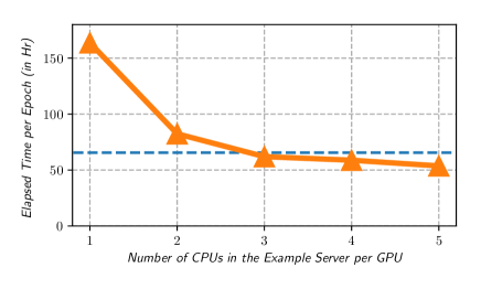
(a)

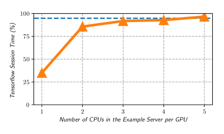
(b)

Fig. 3: The efficiency of the example server with respect to the number of CPUs per GPU: (a) The required time to process a single epoch during the training phase and (b) the percentage of Tensorflow computation time defined by (2). The blue horizontal dotted lines in each figure represent the case when data augmentation with example servers is not employed.

3 Structure of the end-to-end speech recognition system

We have adopted the RETURNN speech recognition system [51, 52] for training our end-to-end system with various modifications. Some of the important modifications are: replacing the input data pipeline with our proposed on-the-fly example server based pipeline with support for VTLP and acoustic simulation, implementing the Monotonic Chunkwise Attention (MoChA) [49] for online streaming end-to-end speech recognition, minimum Word Error Rate (mWER) training, support for handling Korean language or script, our own scoring and Inverse Text Normalization (ITN) modules, support for power mel filterbank features [1, 43], etc. We have tried various types of training strategies for better performance [53, 54]. Our MoCha implementation and optimization are described in very detail in our another paper [50].

The structure of our entire end-to-end speech recognition system is shown in Fig. 2. $\vec{x}[m]$ and $\vec{y}_{l}$ are the input power mel filterbank energy vector and the output label, respectively. $m$ is the input frame index and $l$ is the decoder output step index. $\vec{c}_{l}$ is the context vector calculated as a weighted sum of the encoder hidden state vectors denoted as $\vec{h}^{enc}[m]$. The attention weights are computed as a softmax of energies computed as a function of the encoder hidden state $\vec{h}^{enc}[m]$, the decoder hidden state $\vec{h}^{dec}_{l}$, and the attention weight feedback $\vec{\beta}_{l}[m]$ [52].

In [52], the peak value of the speech waveform is normalized to be one. However, since finding the peak sample value is not possible for online feature extraction, we do not perform this normalization. We modified the input pipeline so that the online feature generation can be performed. We disabled the clipping of feature range between -3 and 3, which is the default setting for the Librispeech experiment using MFCC features in [52]. We conducted experiments using both the uni-directional and bi-directional Long Short-Term Memories (LSTMs) [9] in the encoder. However, only the uni-directional LSTMs are used in the decoder. For online speech recognition experiments, we used the MoChA models [49] with a chunk size of 2. In MoCha experiments, we used only the uni-directional LSTMs both in the encoder and the decoder to enable streaming recognition. For better stability in LSTM training, we use the gradient clipping by global norm [55], which is implemented as tf.clip_by_global_norm API in Tensorflow [38]. We use six layers of encoders and one layer of decoder followed by a softmax layer.

In performing shallow-fusion with an external LM, our approach is slightly different from the previously known approaches [56, 57] to obtain better performance. we used the following equation:

$$y_{0:L}^{*}= \operatorname*{arg\,max}_{y_{0:L}}\sum_{l=0}^{L-1}\Big{[}\log P\left(y_{l}|\vec{x}[0:M],y_{0:l}\right)$$

$$\qquad-\lambda_{p}\log P(y_{l})+\lambda_{\text{lm}}\log P\left(y_{l}|y_{0:l}\right)\Big{]},$$ (3)

where we have an additional term $\lambda_{p}\log P(y_{l})$ for subtracting the prior bias that the model has learned from the training corpus. In (3) $L$ is the length of the output label hypothesis. $\lambda_{p}$ and $\lambda_{\text{lm}}$ are weights for the prior probability and the LM prediction probability, respectively. In (3), we represented sequences following the Python slice notation. For example, $\vec{x}[0:M]$ denotes the sequence of the input acoustic features of length $M$, and $y_{0:L}$ is a sequence of output labels of length $L$.

4 Experimental Results

In this section, we present a summary of experimental results obtained with our end-to-end speech recognition systems built using the proposed Samsung Research end-to-end training framework. For near-field speech recognition experiments, we use the open source Librispeech database [3], as well as our in-house Bixby [11] usage training and test sets for English. The LibriSpeech dataset consists of around 960 hours of training data consisting of 281,241 utterances. The evaluation set consists of the official 5.4 hours test-clean and 5.1 hours test-other data. The Bixby training set consists of approximately 10,000 hours of anonymized Bixby usage data. The evaluation set consists of around 1,000 open domain utterances. As mentioned in Sec. 2.4, we used 8 GPUs in a GPU cluster and 40 CPUs in an example server when training the model using the Bixby training set.

Table 1: Word Error Rates (WERs) obtained using MFCC implemented in [58] and power mel filterbank coefficients
on the Librispeech corpus [3]. For each WER number,
the same experiment was conducted twice and averaged.

Cell Size		MFCC	Power Mel Filterbank Coefficients
1536 cell	test-clean	4.06 %	3.94 %
	test-other	13.97 %	13.56 %
	average	9.02 %	8.75 %

Table 2: Word Error Rates (WERs) obtained with VTLP processing with different warping factor $\alpha$ distribution, and with and without an RNN LM. The warping factor $\alpha$ is the constant controlling warping in (1).

Warping Factor		0.7 $\sim$ 1.3	0.8 $\sim$ 1.2	0.9 $\sim$ 1.1
Without RNN-LM	test-clean	3.82 %	3.66 %	3.86 %
	test-other	12.50 %	12.39 %	12.35 %
	average	8.16 %	8.03 %	8.11 %
With RNN-LM	test-clean	2.93 %	2.85 %	2.96 %
	test-other	10.40 %	10.25 %	10.13 %
	average	6.67 %	6.55 %	6.55 %

In Table 1, we compare the performance between the baseline MFCC and the power-law of $(\cdot)^{\frac{1}{15}}$ features for a Bidirectional Full Attention (BFA) end-to-end model with an LSTM cell size of 1536 on the LibriSpeech database [3]. Especially for test-other, which is a more difficult task, the power mel filterbank coefficients shows better performance than the baseline MFCC. Thus, we use the power-mel filterbank coefficients as the default feature in our end-to-end system. All the following results in this section were obtained using the power-mel filterbank coefficients.

In Table 2, we show Word Error Rates (WERs) on the same LibriSpeech corpus for a BFA model using different window sizes and warping coefficient distributions, with and without using an external Recurrent Neural Network (RNN) Language Model (LM) [52] built using the standard LibriSpeech LM corpus. The best performance was achieved when the window length is 50 ms and the warping coefficients are uniformly distributed between 0.8 and 1.2. We obtained 3.66 % WER on the test-clean database and 12.39 % WER on the test-other database without using an LM. Using this shallow-fusion technique with an RNN-LM, we achieved WERs of 2.85 % and 10.25 % on the Librispeech test-clean and test-other databases, respectively.

Table 3: Word Error Rates (WERs) obtained with VTLP processing using shallow-fusion with a Transformer LM with different beam sizes. The window length is 50 ms, and the warping factor distribution is $0.8\sim 1.2$.

Beam Size	12	24	36	48
$\lambda_{p}$ $\lambda_{\text{lm}}$	0.005 0.45	0.004 0.46	0.003 0.48	0.002 0.48
test-clean	2.49 %	2.45 %	2.44 %	2.45 %
test-other	8.76 %	8.40 %	8.29 %	8.22 %
average	5.63 %	5.43 %	5.37 %	5.34 %

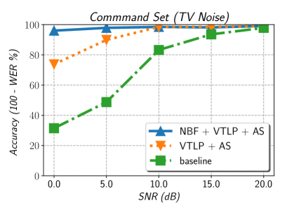
(a)

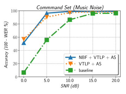
(b)

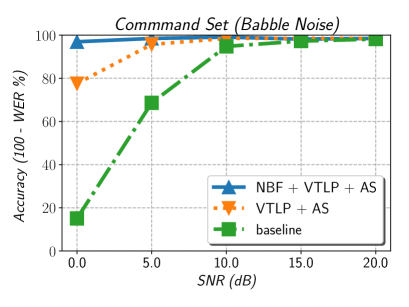
(c)

Fig. 4: Speech recognition accuracy at different Signal-to-Noise Ratios (SNRs) under three different noisy conditions: direct TV noise (a) , music noise (b), and babble noise (c). NBF, VTLP, and AS stand for Neural Beam Former (NBF) [59], Vocal Tract Length Perturbation (VTLP) [1] , and Acoustics Simulator (AS) [2, 36], respectively.

Table 3 shows word error rates on the LibriSpeech testsets obtained by applying shallow-fusion with a Transformer LM [60, 61] using (3). As shown in this table, we conducted experiments with different beam sizes, $\lambda_{p}$ and $\lambda_{\text{lm}}$ parameters in (3). The best result we obtained using a Transformer LM in Table 3 is significantly better than the result we obtained with a LSTM LM in Table 2.

In Table 4, we summarize our WER results for both the LibriSpeech and Bixby end-to-end ASR models. In the case of the Bixby model, we optionally used an external RNN-LM trained using around 65GB of the Bixby LM corpus with an architecture exactly similar to the LibriSpeech LM model used in [52]. The cell sizes of the LibriSpeech model and the Bixby model in Table 4 are 1536 and 1024 respectively. For comparison, the best WFST based conventional LSTM-HMM based ASR system gives a WER of 8.85% on the Bixby same open domain test set. We can see that our current Bixby end-to-end BFA model is $\sim$10% better, while our MoChA streaming model is $\sim$10% poorer compared to the conventional WFST based DNN-HMM system.

Table 4: Summary of Word Error Rates (WERs) obtained for different LibriSpeech and Bixby near-field end-to-end ASR models with and without an RNN LM.

Models		BFA	MoChA
LibriSpeech (1536-cell) test-clean	w/o LM	3.66 %	6.78 %
	RNN-LM	2.85 %	5.54 %
	Transformer LM	2.44 %	-
Bixby (1024-cell)	w/o LM	8.25 %	10.77 %
	RNN-LM	7.92 %	9.95 %

The performance of our far-field end-to-end ASR model trained using the proposed structure in Fig. 2 is shown in Fig. 4. In this experiment, we used the same anonymized 10,000 hours of the English Bixby training set. The performance of the far-field models were evaluated on the English Bixby command test set. The Bixby command test set include utterancesare sampled from the anonymized Bixby usage log. Examples in this test set include “Set an alarm for tomorrow at 6 a.m”, “Tell me remaining time of my timers”, “Play the most latest added song”, and so on.

Far-field recording using this Bixby command set was performed by playing back utterances using a loud speaker at 5-meter distance in a real room. The reverberation time in this recording room was measured to be $T_{60}=430ms$. We used two microphones on a prototype Galaxy Home Mini to record this far-field speech. The distance between two microphones is 6.8 cm. We simulated far-field additive noise by playing back three different types of noise using loud speakers. In Fig. 4(a), we used a single loud speaker located at 1-meter distance from the microphone to simulate direct noise from a television. In Figs. 4(b) and 4(c), we used four loud speakers oriented to different directions to simulate diffuse noise. On the prototype Galaxy home Mini device, the two-microphone signals are enhanced using a beamformer based on the Neural Network supported Generalized Eigenvalue (NN-GEV) algorithm [59]. In Fig. 4, we evaluated speech recognition accuracy using three different systems. NBP+VTLP+AS denotes a system which uses the VTLP system and the acoustic simulator described in this paper for data augmentation in model training, and additionally uses this NN-GEV-based beamformer for signal enhancement. NBF in this future stands for this Neural Beam Former (NBF). VTLP+AS denotes a system employing the VTLP system and the acoustic simulator without using this beamformer. baseline denotes a system which was trained using utterances recorded in close-talking environments without any further processing. As can be seen in these figures, data augmentation technique significantly enhances speech recognition accuracy under the far-field environments. We also observe that the data augmentation algorithm described in Sec. 2 does not harm the clean performance, thus we may use the same data augmentation both for the close-talking and the far-field environments. In case of the direct TV noise in Fig. 4(a) and babble noise in Fig. 4(c), we observe that further improvement is achieved by employing a NN-GEV-based beamformer.

5 Conclusions

We presented a new end-to-end training framework and strategies for training state-of-the-art end-to-end speech recognition systems. Our training system utilizes a cluster of Central Processing Units (CPUs) and Graphics Processing Units (GPUs). The entire data reading, large scale data augmentation, neural network parameter updates are performed on-the-fly using example servers and sharded TFRecords and tf.data. We use vocal tract length perturbation and an acoustic simulator for data augmentation. Horovod allreduce approach is employed to train the neural network parameters using Adam optimizer. We evaluated the effectiveness of our system on the standard Librispeech corpus [3] and 10,000-hr anonymized Bixby English training and test sets both in near-field as well as far-field scenarios.

References

- [1] C. Kim, M. Shin, A. Garg, and D. Gowda, “Improved Vocal Tract Length Perturbation for a State-of-the-Art End-to-End Speech Recognition System,” in INTERSPEECH-2019, Graz, Austria, Sept. 2019, pp. 739–743. [Online]. Available: http://dx.doi.org/10.21437/Interspeech.2019-3227
- [2] C. Kim, A. Misra, K. Chin, T. Hughes, A. Narayanan, T. N. Sainath, and M. Bacchiani, “Generation of large-scale simulated utterances in virtual rooms to train deep-neural networks for far-field speech recognition in google home,” in Proc. Interspeech 2017, 2017, pp. 379–383. [Online]. Available: http://dx.doi.org/10.21437/Interspeech.2017-1510
- [3] V. Panayotov, G. Chen, D. Povey, and S. Khudanpur, “Librispeech: An asr corpus based on public domain audio books,” in IEEE Int. Conf. Acoust., Speech, and Signal Processing, April 2015, pp. 5206–5210.
- [4] M. Seltzer, D. Yu, and Y.-Q. Wang, “An investigation of deep neural networks for noise robust speech recognition,” in Int. Conf. Acoust. Speech, and Signal Processing, 2013, pp. 7398–7402.
- [5] D. Yu, M. L. Seltzer, J. Li, J.-T. Huang, and F. Seide, “Feature learning in deep neural networks - studies on speech recognition tasks,” in Proceedings of the International Conference on Learning Representations, 2013.
- [6] V. Vanhoucke, A. Senior, and M. Z. Mao, “Improving the speed of neural networks on CPUs,” in Deep Learning and Unsupervised Feature Learning NIPS Workshop, 2011.
- [7] G. Hinton, L. Deng, D. Yu, G. E. Dahl, A. Mohamed, N. Jaitly, A. Senior, V. Vanhoucke, P. Nguyen, T. Sainath, and B. Kingsbury, “Deep neural networks for acoustic modeling in speech recognition: The shared views of four research groups,” IEEE Signal Processing Magazine, vol. 29, no. 6, Nov. 2012.
- [8] T. Sainath, R. J. Weiss, K. W. Wilson, B. Li, A. Narayanan, E. Variani, M. Bacchiani, I. Shafran, A. Senior, K. Chin, A. Misra, and C. Kim, “Multichannel signal processing with deep neural networks for automatic speech recognition,” IEEE/ACM Trans. Audio, Speech, Lang. Process., Feb. 2017.
- [9] S. Hochreiter and J. Schmidhuber, “Long short-term memory,” Neural Computation, no. 9, pp. 1735–1780, Nov. 1997.
- [10] B. Li, T. Sainath, A. Narayanan, J. Caroselli, M. Bacchiani, A. Misra, I. Shafran, H. Sak, G. Pundak, K. Chin, K-C Sim, R. Weiss, K. Wilson, E. Variani, C. Kim, O. Siohan, M. Weintraub, E. McDermott, R. Rose, and M. Shannon, “Acoustic modeling for Google Home,” in INTERSPEECH-2017, Aug. 2017, pp. 399–403.
- [11] “Samsung bixby,” http://www.samsung.com/bixby/.
- [12] W. Chan, N. Jaitly, Q. Le, and O. Vinyals, “Listen, attend and spell: A neural network for large vocabulary conversational speech recognition,” in 2016 IEEE International Conference on Acoustics, Speech and Signal Processing (ICASSP), March 2016, pp. 4960–4964.
- [13] R. Prabhavalkar, K. Rao, T. N. Sainath, B. Li, L. Johnson, and N. Jaitly, “A comparison of sequence-to-sequence models for speech recognition,” in Proc. Interspeech 2017, 2017, pp. 939–943. [Online]. Available: http://dx.doi.org/10.21437/Interspeech.2017-233
- [14] J. K. Chorowski, D. Bahdanau, D. Serdyuk, K. Cho, and Y. Bengio, “Attention-based models for speech recognition,” in Advances in Neural Information Processing Systems 28, C. Cortes, N. D. Lawrence, D. D. Lee, M. Sugiyama, and R. Garnett, Eds. Curran Associates, Inc., 2015, pp. 577–585. [Online]. Available: http://papers.nips.cc/paper/5847-attention-based-models-for-speech-recognition.pdf
- [15] C.-C. Chiu, T. N. Sainath, Y. Wu, R. Prabhavalkar, P. Nguyen, Z. Chen, A. Kannan, R. J. Weiss, K. Rao, E. Gonina, N. Jaitly, B. Li, J. Chorowski, and M. Bacchiani, “State-of-the-art speech recognition with sequence-to-sequence models,” in 2018 IEEE International Conference on Acoustics, Speech and Signal Processing (ICASSP), April 2018, pp. 4774–4778.
- [16] R. Prabhavalkar, T. N. Sainath, Y. Wu, P. Nguyen, Z. Chen, C. Chiu, and A. Kannan, “Minimum word error rate training for attention-based sequence-to-sequence models,” in 2018 IEEE International Conference on Acoustics, Speech and Signal Processing (ICASSP), April 2018, pp. 4839–4843.
- [17] A. Narayanan, A. Misra, K. C. Sim, G. Pundak, A. Tripathi, M. Elfeky, P. Haghani, T. Strohman, and M. Bacchiani, “Toward domain-invariant speech recognition via large scale training,” in 2018 IEEE Spoken Language Technology Workshop (SLT), Dec 2018, pp. 441–447.
- [18] H. Soltau, H. Liao, and H. Sak, “Neural speech recognizer: Acoustic-to-word lstm model for large vocabulary speech recognition,” in INTERSPEECH-2017, 2017, pp. 3707–3711. [Online]. Available: http://dx.doi.org/10.21437/Interspeech.2017-1566
- [19] E. Variani, T. Bagby, E. McDermott, and M. Bacchiani, “End-to-end training of acoustic models for large vocabulary continuous speech recognition with tensorflow,” in INTERSPEECH-2017, 2017, pp. 1641–1645. [Online]. Available: http://dx.doi.org/10.21437/Interspeech.2017-1284
- [20] P. Goyal, P. Dollár, R. B. Girshick, P. Noordhuis, L. Wesolowski, A. Kyrola, A. Tulloch, Y. Jia, and K. He, “Accurate, large minibatch SGD: training imagenet in 1 hour,” CoRR, vol. abs/1706.02677, 2017. [Online]. Available: http://arxiv.org/abs/1706.02677
- [21] C. Kim and R. M. Stern, “Power-Normalized Cepstral Coefficients (PNCC) for Robust Speech Recognition,” IEEE/ACM Trans. Audio, Speech, Lang. Process., pp. 1315–1329, July 2016.
- [22] U. H. Yapanel and J. H. L. Hansen, “A new perceptually motivated MVDR-based acoustic front-end (PMVDR) for robust automatic speech recognition,” Speech Communication, vol. 50, no. 2, pp. 142–152, Feb. 2008.
- [23] C. Kim, K. Chin, M. Bacchiani, and R. M. Stern, “Robust speech recognition using temporal masking and thresholding algorithma,” in INTERSPEECH-2014, Sept. 2014, pp. 2734–2738.
- [24] T. Nakatani, N. Ito, T. Higuchi, S. Araki, and K. Kinoshita, “Integrating DNN-based and spatial clustering-based mask estimation for robust MVDR beamforming,” in IEEE Int. Conf. Acoust., Speech, Signal Processing, March 2017, pp. 286–290.
- [25] T. Higuchi and N. Ito and T. Yoshioka and T. Nakatani, “Robust MVDR beamforming using time-frequency masks for online/offline ASR in noise,” in IEEE Int. Conf. Acoust., Speech, Signal Processing, March 2016, pp. 5210–5214.
- [26] H. Erdogan, J. R. Hershey, S. Watanabe, M. Mandel, J. Roux, “Improved MVDR Beamforming Using Single-Channel Mask Prediction Networks,” in INTERSPEECH-2016, Sept 2016, pp. 1981–1985.
- [27] C. Kim, K. Eom, J. Lee, and R. M. Stern, “Automatic selection of thresholds for signal separation algorithms based on interaural delay,” in INTERSPEECH-2010, Sept. 2010, pp. 729–732.
- [28] C. Kim, C. Khawand, and R. M. Stern, “Two-microphone source separation algorithm based on statistical modeling of angle distributions,” in IEEE Int. Conf. on Acoustics, Speech, and Signal Processing, March 2012, pp. 4629–4632.
- [29] C. Kim and K. K. Chin, “Sound source separation algorithm using phase difference and angle distribution modeling near the target,” in INTERSPEECH-2015, Sept. 2015, pp. 751–755.
- [30] C. Kim, A. Menon, M. Bacchiani, and R. Stern, “Sound source separation using phase difference and reliable mask selection selection,” in 2018 IEEE International Conference on Acoustics, Speech and Signal Processing (ICASSP), April 2018, pp. 5559–5563.
- [31] R. Lippmann, E. Martin, and D. Paul, “Multi-style training for robust isolated-word speech recognition,” in IEEE International Conference on Acoustics, Speech, and Signal Processing, vol. 12, Apr 1987, pp. 705–708.
- [32] C. Kim, T. Sainath, A. Narayanan, A. Misra, R. Nongpiur, and M. Bacchiani, “Spectral distortion model for training phase-sensitive deep-neural networks for far-field speech recognition,” in 2018 IEEE International Conference on Acoustics, Speech and Signal Processing (ICASSP), April 2018, pp. 5729–5733.
- [33] W. Hartmann, T. Ng, R. Hsiao, S. Tsakalidis, and R. Schwartz, “Two-stage data augmentation for low-resourced speech recognition,” in INTERSPEECH-2016, 2016, pp. 2378–2382. [Online]. Available: http://dx.doi.org/10.21437/Interspeech.2016-1386
- [34] D. S. Park, W. Chan, Y. Zhang, C.-C. Chiu, B. Zoph, E. D. Cubuk, and Q. V. Le, “SpecAugment: A Simple Data Augmentation Method for Automatic Speech Recognition,” in Proc. Interspeech 2019, 2019, pp. 2613–2617. [Online]. Available: http://dx.doi.org/10.21437/Interspeech.2019-2680
- [35] C. Kim, K. Kumar and R. M. Stern, “Robust speech recognition using small power boosting algorithm,” in IEEE Automatic Speech Recognition and Understanding Workshop, Dec. 2009, pp. 243–248.
- [36] C. Kim, E. Variani, A. Narayanan, and M. Bacchiani, “Efficient implementation of the room simulator for training deep neural network acoustic models,” in INTERSPEECH-2018, Sept 2018, pp. 3028–3032. [Online]. Available: http://dx.doi.org/10.21437/Interspeech.2018-2566
- [37] N. Jaitly and G. E. Hinton, “Vocal tract length perturbation (vtlp) improves speech recognition,” in Int. Conf. Mach. Learn. (ICML) Workshop on Deep Learn. Audio, Speech, Lang. Process., 2013.
- [38] M. Abadi, P. Barham, J. Chen, Z. Chen, A. Davis, J. Dean, M. Devin, S. Ghemawat, G. Irving, M. Isard, M. Kudlur, J. Levenberg, R. Monga, S. Moore, D. G. Murray, B. Steiner, P. Tucker, V. Vasudevan, P. Warden, M. Wicke, Y. Yu, and X. Zheng, “Tensorflow: A system for large-scale machine learning,” in 12th USENIX Symposium on Operating Systems Design and Implementation (OSDI 16). Savannah, GA: USENIX Association, 2016, pp. 265–283. [Online]. Available: https://www.usenix.org/conference/osdi16/technical-sessions/presentation/abadi
- [39] A. Sergeev and M. D. Balso, “Horovod: fast and easy distributed deep learning in TensorFlow,” arXiv preprint arXiv:1802.05799, 2018.
- [40] IBM, IBM Spectrum LSF, Version 10 Release 1.0, Configuration Reference.
- [41] X. Cui, V. Goel, and B. Kingsbury, “Data augmentation for deep neural network acoustic modeling,” IEEE/ACM Transactions on Audio, Speech, and Language Processing, vol. 23, no. 9, pp. 1469–1477, Sept 2015.
- [42] P. Zhan and A. Waibel, “Vocal tract length normalization for large vocabulary continuous speech recognition,” School of Computer Science, Carnegie Mellon University, Tech. Rep. CMU-CS-97-148, May 1997. [Online]. Available: https://www.lti.cs.cmu.edu/sites/default/files/CMU-LTI-97-150-T.pdf
- [43] C. Kim, M. Kumar, K. Kim, and D. Gowda, “Power-law nonlinearity with maximally uniform distribution criterion for improved neural network training in automatic speech recognition,” in 2019 IEEE Automatic Speech Recognition and Understanding Workshop (ASRU), Dec. 2019 (accepted).
- [44] C. Kim and R. M. Stern, “Feature extraction for robust speech recognition based on maximizing the sharpness of the power distribution and on power flooring,” in IEEE Int. Conf. on Acoustics, Speech, and Signal Processing, March 2010, pp. 4574–4577.
- [45] ——, “Power-normalized cepstral coefficients (pncc) for robust speech recognition,” in IEEE Int. Conf. on Acoustics, Speech, and Signal Processing, March 2012, pp. 4101–4104.
- [46] C. Kim, “Signal processing for robust speech recognition motivated by auditory processing,” Ph.D. dissertation, Carnegie Mellon University, Pittsburgh, PA USA, Dec. 2010.
- [47] C. Kim and R. M. Stern, “Feature extraction for robust speech recognition using a power-law nonlinearity and power-bias subtraction,” in INTERSPEECH-2009, Sept. 2009, pp. 28–31.
- [48] “Zero mq,” http:zeromq.org.
- [49] C.-C. Chiu and C. Raffel, “Monotonic chunkwise attention,” in International Conference on Learning Representations, Apr. 2018. [Online]. Available: https://openreview.net/forum?id=Hko85plCW
- [50] K. Kim, K. Lee, D. Gowda, J. Park, S. Kim, S. Jin, Y.-Y. Lee, J. Yeo, D. Kim, S. Jung, J. Lee, M. Han, and C. Kim, “attention based on-device streaming speech recognition with large speech corpus,” in 2019 IEEE Automatic Speech Recognition and Understanding Workshop (ASRU), Dec. 2019 (accepted).
- [51] P. Doetsch, A. Zeyer, P. Voigtlaender, I. Kulikov, R. Schlüter, and H. Ney, “RETURNN: the RWTH extensible training framework for universal recurrent neural networks,” in IEEE Int. Conf. Acoust., Speech, and Signal Processing, March 2017, pp. 5345–5349.
- [52] A. Zeyer, K. Irie, R. Schlüter, and H. Ney, “Improved training of end-to-end attention models for speech recognition,” in INTERSPEECH-2018, 2018, pp. 7–11. [Online]. Available: http://dx.doi.org/10.21437/Interspeech.2018-1616
- [53] D. Gowda, A. Garg, K. Kim, M. Kumar, and C. Kim, “Multi-task multi-resolution char-to-bpe cross-attention decoder for end-to-end speech recognition,” in INTERSPEECH-2019, Graz, Austria, Sept. 2019, pp. 2783–2787. [Online]. Available: http://dx.doi.org/10.21437/Interspeech.2019-3216
- [54] A. Garg, D. Gowda, A. Kumar, K. Kim, M. Kumar, and C. Kim, “Improved multi-stage training of online attention-based encoder-decoder models,” in 2019 IEEE Automatic Speech Recognition and Understanding Workshop (ASRU), Dec. 2019 (accepted).
- [55] R. Pascanu, T. Mikolov, and Y. Bengio, “On the difficulty of training recurrent neural networks,” in Proceedings of the 30th International Conference on International Conference on Machine Learning - Volume 28, ser. ICML’13. JMLR.org, 2013, pp. III–1310–III–1318. [Online]. Available: http://dl.acm.org/citation.cfm?id=3042817.3043083
- [56] Ç. Gülçehre, O. Firat, K. Xu, K. Cho, L. Barrault, H. Lin, F. Bougares, H. Schwenk, and Y. Bengio, “On using monolingual corpora in neural machine translation,” CoRR, vol. abs/1503.03535, 2015. [Online]. Available: http://arxiv.org/abs/1503.03535
- [57] S. Toshniwal, A. Kannan, C. Chiu, Y. Wu, T. N. Sainath, and K. Livescu, “A comparison of techniques for language model integration in encoder-decoder speech recognition,” in 2018 IEEE Spoken Language Technology Workshop (SLT), Dec 2018, pp. 369–375.
- [58] B. McFee, C. Raffel, D. Liang, D. P. Ellis, M. McVicar, E. Battenberg, and O. Nieto, “librosa: Audio and music signal analysis in python,” in Proceedings of the 14th Python in Science Conference, K. Huff and J. Bergstra, Eds., 2015, pp. 18 – 25.
- [59] J. Heymann, L. Drude, and R. Haeb-Umbach, “Neural network based spectral mask estimation for acoustic beamforming,” in 2016 IEEE International Conference on Acoustics, Speech and Signal Processing (ICASSP), March 2016, pp. 196–200.
- [60] A. Vaswani, N. Shazeer, N. Parmar, J. Uszkoreit, L. Jones, A. N. Gomez, L. u. Kaiser, and I. Polosukhin, “Attention is all you need,” in Advances in Neural Information Processing Systems 30, I. Guyon, U. V. Luxburg, S. Bengio, H. Wallach, R. Fergus, S. Vishwanathan, and R. Garnett, Eds. Curran Associates, Inc., 2017, pp. 5998–6008. [Online]. Available: http://papers.nips.cc/paper/7181-attention-is-all-you-need.pdf
- [61] C. Lüscher, E. Beck, K. Irie, M. Kitza, W. Michel, A. Zeyer, R. Schlüter, and H. Ney, “RWTH ASR systems for librispeech: Hybrid vs attention - w/o data augmentation,” CoRR, vol. abs/1905.03072, 2019. [Online]. Available: http://arxiv.org/abs/1905.03072