The trident process in laser pulses

Abstract

We study the trident process in laser pulses. We provide exact numerical results for all contributions, including the difficult exchange term. We show that all terms are in general important for a short pulse. For a long pulse we identify a term that gives the dominant contribution even if the intensity is only moderately high, $a_{0}\gtrsim 1$, which is an experimentally important regime where the standard locally-constant-field (LCF) approximation cannot be used. We show that the spectrum has a richer structure at $a_{0}\sim 1$, compared to the LCF regime $a_{0}\gg 1$. We study the convergence to LCF as $a_{0}$ increases and how this convergence depends on the momentum of the initial electron. We also identify the terms that dominate at high energy.

I Introduction

The trident process, $e^{\scriptscriptstyle-}\to 2e^{\scriptscriptstyle-}+e^{\scriptscriptstyle+}$, in laser fields has recently attracted renewed interest Dinu:2017uoj ; King:2018ibi ; Mackenroth:2018smh ; Acosta:2019bvh ; Krajewska15 ; Hu:2014ooa following King:2013osa ; Ilderton:2010wr ; Hu:2010ye and the classic experiment at SLAC Bamber:1999zt . While this process was studied already in the early seventies Ritus:1972nf ; Baier , it is only with modern high-intensity lasers that it is becoming experimentally important. Although the SLAC experiment is already two decades old and there today exist much stronger lasers, it is still the only experiment directly relevant for this process. This, however, will likely change soon, given the great deal of interest in this process in itself desyWorkshop ; LUXEparameters ; Abramowicz:2019gvx ; MeurenPresentation and as a first step towards production of many particles in cascades Bell:2008zzb ; Elkina:2010up ; Nerush:2010fe . A related second-order process is double nonlinear Compton scattering Morozov:1975uah ; Lotstedt:2009zz ; Loetstedt:2009zz ; Seipt:2012tn ; Mackenroth:2012rb ; King:2014wfa ; Dinu:2018efz ; Wistisen:2019pwo , where the electron instead produces two photons.

We use units with $c=\hbar=m_{e}=1$, where $m_{e}$ is the electron mass, and we absorb a factor the charge $e$ into the background field, so $e$ only appears explicitly via the coupling $\alpha$ to the quantized field. The trident process depends on $a_{0}=E/\omega$, where $E$ is the field strength and $\omega$ the characteristic frequency of the plane-wave background field, and $\chi=a_{0}b_{0}$, where $b_{0}=kp$ is the product of the wave vector of the plane wave, $k_{\mu}$ with $k_{0}=\omega$, and the momentum of the initial electron $p_{\mu}$.

The trident process can be separated into one-step and two-step parts, where the latter is obtained from an incoherent product of nonlinear Compton scattering and nonlinear Breit-Wheeler pair production. If the intensity of the background is sufficiently high then one can approximate the trident probability by the two-step where the field is treated as locally constant at the two steps. This locally constant field (LCF) approximation greatly simplifies the calculation and also makes it possible to approximate complicated higher-order processes by a sequence of first-order processes using particle-in-cell codes RidgersCode ; Gonoskov:2014mda ; Osiris ; Smilei . However, the LCF approximation can break down at both low and high energies Dinu:2015aci ; DiPiazza:2017raw ; Podszus:2018hnz ; Ilderton:2019kqp . Moreover, this also means that one misses much of the additional structure in the trident probability that is not already in the LCF approximation of the two first-order processes. This gives motivation for studying fields with moderately high intensity.

In this paper we consider the trident process at moderately high intensity, i.e. $a_{0}\gtrsim 1$. In this regime we can neither make a perturbative expansion in $a_{0}$ nor employ the LCF approximation, which is basically an expansion in $1/a_{0}\ll 1$ Dinu:2017uoj . As we showed in Dinu:2017uoj , for $a_{0}\sim 1$ the one-step terms are in general on the same order of magnitude as the two-step term, and then one in general has to include the exchange term, i.e. the cross-term between the two terms in the amplitude that are related by exchanging the two electrons in the final state. The exchange term is much harder to calculate than the direct terms, i.e. the non-exchange terms. So, it is important to know in which parameter regimes one can neglect the exchange term. We study this here.

While the trident process has been observed in Bamber:1999zt , there the laser only had a small $a_{0}$ and they found a probability that scaled as $a_{0}$ to the power of the number of photons that need to be absorbed to produce a pair. While that observation was already nonlinear in $a_{0}$, for higher intensities the dependence on the field strength becomes more interesting. For $a_{0}\gg 1$ and $\chi\ll 1$ one finds a probability that scales as Ritus:1972nf ; Baier

$$\mathbb{P}\sim\exp\left(-\frac{16}{3\chi}\right)\;.$$ (1)

This scaling is basically the same as for the nonperturbative Sauter-Schwinger process Sauter:1931zz ; Heisenberg:1935qt ; Schwinger:1951nm , cf. Bamber:1999zt , where the probability of spontaneous pair production by a constant electric field scales as

$$\mathbb{P}\sim\exp\left(-\frac{\pi}{E}\right)\;.$$ (2)

Since in the trident case we have $\chi=E$ in the rest frame of the initial electron, the difference between (1) and (2) is basically just a numerical factor. There is a similar scaling for nonlinear Breit-Wheeler pair production Reiss62 ; Nikishov:1964zza ; Hartin:2018sha

$$\mathbb{P}\sim\exp\left(-\frac{8}{3\chi_{\gamma}}\right)\;,$$ (3)

where $\chi_{\gamma}=a_{0}kl$ is proportional to the momentum $l_{\mu}$ of the initial photon. However, in this case there is no frame in which $\chi_{\gamma}$ is equal to the field strength, it always contains the frequency of the initial photon. The advantage of Breit-Wheeler, as well as other photon/field-assisted mechanisms Schutzhold:2008pz ; Dunne:2009gi , is that one has production of matter from an initial state with only photons. The advantage of the trident process is that one finds an exponential scaling with an even closer resemblance to the elusive Sauter-Schwinger process. This provides further motivation for studying the trident process with upcoming high-intensity laser facilities, such as LUXE LUXEparameters ; Abramowicz:2019gvx and FACET-II MeurenPresentation .

This can be generalized to inhomogeneous fields. In the trident case we find Dinu:2017uoj for $a_{0}\gtrsim 1$ and $\chi\ll 1$ $\mathbb{P}\sim\exp\left(-f(a_{0})/\chi\right)$ with some function $f$ which depends on the field shape, and in the Sauter-Schwinger case one finds, for a time-dependent electric field with frequency $\omega$ and $E\ll 1$, $\mathbb{P}\sim\exp\left(-F(\gamma)/E\right)$, where the dependence on $\omega$ is in this context usually expressed in terms of the Keldysh parameter $\gamma=\omega/E$, which corresponds to $1/a_{0}$.

In our previous paper Dinu:2017uoj we studied the trident process in plane-wave background fields with the lightfront approach and by integrating over the transverse momentum components as well as summing over all the spins. The advantage of this approach is that the result only depends on relatively few parameters, viz. the field parameters and the longitudinal momentum components. This approach also allowed us to derive relatively compact expressions for the probability for arbitrary field shapes. In this paper we will use these expressions as a starting point for further investigation into the relative importance of the various terms.

This paper is organized as follows. In Sec. II we give some basic definitions. In Sec. III we study numerically the trident spectrum for a pulsed oscillating field. We study the dependence on pulse length, energy parameter $b_{0}$ and $a_{0}$. We have studied the contribution from all one-step terms, including the difficult exchange term, for $a_{0}\gtrsim 1$ i.e. beyond the LCF regime. In Sec. IV and Appendix A we describe our numerical methods.

II Formalism

We use lightfront variables defined by $v^{\scriptscriptstyle\pm}=2v_{\scriptscriptstyle\mp}=v^{0}\pm v^{3}$, $v_{\scriptscriptstyle\perp}=\{v_{1},v_{2}\}$ and $\phi=kx=\omega x^{\scriptscriptstyle+}$. The field is given by $a_{\scriptscriptstyle\perp}(\phi)$. The initial electron has momentum $p^{\mu}$, and the final state electrons and positron have momenta $p_{1,2}^{\mu}$ and $p_{3}^{\mu}$, respectively. The quantities we are interested in here only depend on the longitudinal momentum components of the fermions, which we denote as $b_{0}=kp$ and $s_{i}=kp_{i}/kp$. We also use $q_{i}:=1-s_{i}$, $i=1,2$ for the longitudinal momentum of the intermediate photon.

We consider either the integrated probability $\mathbb{P}$ or the longitudinal momentum spectrum $\mathbb{P}(s)$, which are related via

$$\mathbb{P}=\int_{0}^{1}\mathrm{d}s_{1}\mathrm{d}s_{2}\theta(s_{3})\mathbb{P}(s)\;.$$ (4)

These are obtained by performing the Gaussian integrals over the transverse momenta $p_{1{\scriptscriptstyle\perp}}$ and $p_{2{\scriptscriptstyle\perp}}$. We can perform these integrals analytically for any field shape, so it is a natural step in order to reduce the number of independent parameters. From an experimental point of view, it is also worth noting that in an electron-laser collision, the initial electron will in most cases have a very large $\gamma$ factor. This means that the produced particles will travel almost parallel to the initial momentum. So, although we have integrated over all possible values of the transverse momenta, the dominant contribution comes from a relatively small region around the forward direction, see Appendix B. So, performing these transverse integrals effectively gives what a detector around the forward Gaussian peak would measure. So, for high energies the ratios of longitudinal momenta $s_{i}$ also give us the fraction of the initial electron’s momentum/energy given to the produced particles.

The amplitude has two terms, $M_{12}$ and $M_{21}$, where $M_{21}$ is obtained from $-M_{12}$ by swapping place of the two identical electrons in the final state. On the probability level $|M_{12}|^{2}$ and $|M_{21}|^{2}$ give what we call the direct part $\mathbb{P}_{\rm dir}$, and $2\text{Re }M_{21}^{*}M_{12}$ gives the exchange part $\mathbb{P}_{\rm ex}$. Note that “direct” does not mean instantaneous. In fact, $\mathbb{P}_{\rm dir}=\mathbb{P}_{\rm two}+\mathbb{P}_{\rm one}^{\rm dir}$ gives the entire two-step $\mathbb{P}_{\rm two}$ as well as one part of the one-step $\mathbb{P}_{\rm one}^{\rm dir}$. The exchange term only contributes to the one-step $\mathbb{P}_{\rm ex}=\mathbb{P}_{\rm one}^{\rm ex}$. These three terms can be compared with the results from other approaches. In our approach we find it convenient to further split $\mathbb{P}_{\rm one}^{\rm dir}$ and $\mathbb{P}_{\rm one}^{\rm ex}$ each into three parts,

$$\mathbb{P}_{\rm dir}^{\rm one}=\mathbb{P}_{\rm dir}^{11}+\mathbb{P}_{\rm dir}^{12}+\mathbb{P}_{\rm dir}^{22\to 1}$$ (5)

and

$$\mathbb{P}_{\rm ex}=\mathbb{P}_{\rm ex}^{11}+\mathbb{P}_{\rm ex}^{12}+\mathbb{P}_{\rm ex}^{22}\;.$$ (6)

All the contributions to the trident probability are given by the expressions in Appendix B.

Figure 1: All contributions for a short pulse, $\mathcal{T}=\pi$. Dashed lines for LCF and dot-dashed lines for LCF+1.

Figure 2: All one-step contributions and the sum of all contributions for a long pulse, $\mathcal{T}=80$.

Figure 3: The spectrum for the long pulse. $a_{0}=\{1,2,4\}$ in column $\{1,2,3\}$, $\chi=\{1/2,1,2,4,8,16\}$ from top to bottom.

III Numerical study of the trident spectra

In this section we will present a numerical investigation of the trident process for oscillating fields with Gaussian envelope,

$${\bm{a}}(\phi)=a_{0}\{\cos\xi\sin(\phi-\phi_{0}),\sin\xi\cos(\phi-\phi_{0}),0\}e^{-(\phi/\mathcal{T})^{2}}\;.$$ (7)

We may vary the polarization, between linear ($\xi=0$) and circular ($\xi=\pi/4$), as well as the CEP, $\phi_{0}$. We focus on the choices $\xi=0$ and $\phi_{0}=0$ for they give more structure, provide a tougher numerical challenge and strengthen the importance of one-step terms. To reveal the importance of pulse length we have considered both an ultra-short pulse ($\mathcal{T}=\pi$), which maximizes the contribution of the one-step terms, and a longer, realistic pulse ($\mathcal{T}=80$), motivated by state-of-the-art lasers like the ones to be used in LUXE LUXEparameters and FACET-II MeurenPresentation . It might be useful to consider a somewhat shorter pulse if, as in the SLAC experiment, the electron and laser beams collide at a nonzero angle, which would give a shorter effective pulse length. For $a_{0}\geq 1$ and $\chi<1$ we also notice that, unless a pulse with a flat-top envelope is used, the exponential suppression of the rates associated with lower local $\chi(\phi)=a^{\prime}(\phi)b_{0}$ values means that only those peaks that are close to the global maximum contribute significantly, hence the field has a shorter effective length.

Fig. 1 shows the $s_{1}=s_{2}$ and $s_{2}=s_{3}$ cross-sections through the probability density $P\left(s\right)$ for the short pulse, detailing all terms that contribute, their LCF approximation and the improved LCF+1 approximation. LCF+1 is obtained by including the next-to-leading order correction in an expansion in $1/a_{0}$, cf. Dinu:2017uoj ; Ilderton:2018nws . The values $a_{0}=\left(1,~{}2,~{}4\right)$ and $\chi=a_{0}b_{0}=\left(0.5,~{}1,~{}2,~{}4,~{}8\right)$ are considered. Fig. 2] shows the same for the long pulse, apart from the two-step term which can be close to the total probability density and was removed to reduce clutter. Only the one-step terms are shown explicitely. Fig. 3 shows 3D plots of the spectrum for the long pulse, scaled by dividing by $a_{0}^{2}$. For Fig. 2 and 3 we go up to $\chi=16$, as a larger $b_{0}$ value is needed to find an important contribution of the one-step terms for a longer pulse. In Fig. 4 we considered subunitary $a_{0}$ values for the short pulse, scaled by dividing by $a_{0}^{2}$.

To produce the plots in Fig. 2] we approximated the computationally intensive but small $\mathbb{P}_{\rm ex}^{22}\left(s\right)$ by its LCF approximation. The short pulse results of Fig. 1 and the tests we made for longer pulses suggest that this leads to a small error for the $a_{0}=1$ plots and a very small one for higher $a_{0}$. Compare this to the larger discrepancy caused by, for instance, neglecting the focusing of the laser or by the imperfect control of the pulse shape allowed by experiments. Also notice that $\mathbb{P}_{\rm ex}^{22}\left(s\right)$ does not posess those high amplitude oscillations which make $\mathbb{P}_{\rm dir}^{22\rightarrow 1}\left(s\right)$ larger in magnitude than its LCF values for a long pulse, even at low $b_{0}$. We feel that the modest loss of precision of the result due to the approximation we made hardly justifies the use of the great computing power needed to precisely plot $\mathbb{P}_{\rm ex}^{22}\left(s\right)$ on the detailed grid, with many $s$ points. Considering a long, linearly polarized, pulse with subunitary $a_{0}$ is a computationally intensive challenge for the future, as $\mathbb{P}_{\rm ex}^{22}\left(s\right)$ can be very important in that case and has to be computed accurately for a good precision of the total result. The contribution to the spectrum of all the terms but $\mathbb{P}_{\rm ex}^{22}\left(s\right)$ can be computed precisely at arbitrarily high resolution, through the two/three-tiered approach ${\rm A}_{2}$, building intermediate tables to be reused again and again. Thus we were able to produce the high resolution 3D plots of Fig. 3 for the long pulse.

We next present the main conclusions we have drawn from our numerical investigations. The “glued-up” term $\mathbb{P}_{\rm dir}^{22}\left(s\right)$ is the most important, clearly dominates for a long pulse unless $a_{0}$ is subunitary. Our interest in the gluing techniques comes from the conjecture that this can generalize to other processes, see Dinu:2018efz ; gluingPaper , including the ones involving the emission of hard photons.

While good in the LCF limit, the division into steps $\mathbb{P}_{\rm dir}^{22}\left(s\right)=\mathbb{P}_{\rm dir}^{22\to 1}\left(s\right)+\mathbb{P}_{\rm dir}^{22\to 2}\left(s\right)$ adds spurious oscillations to $\mathbb{P}_{\rm dir}^{22\to 1}\left(s\right)$ and $\mathbb{P}_{\rm dir}^{22\to 2}\left(s\right)$ outside LCF. They can be seen in the dependence on both  $a_{0}$ and $s$. Integrating over $s$ smooths out the former. The same oscillations were seen for the corresponding “rates” defined in Dinu:2017uoj . Hence, as $a_{0}$ increases we see much faster convergence for the undivided $\mathbb{P}_{\rm dir}^{22}\left(s\right)$ than for $\mathbb{P}_{\rm dir}^{22\to 1}\left(s\right)$ and $\mathbb{P}_{\rm dir}^{22\to 2}\left(s\right)$ or the “rate”. Thus, away from the LCF limit it is natural to study $\mathbb{P}_{\rm dir}^{22}\left(s\right)$ as whole.

However, there is a way to divide integrals discussed in Appendix A, $I=$ $I^{aa}$ $+$ $I^{a0}+I^{0a}$, which is elegant, efficient and smooth, adding no such oscillations to its terms. It originates in the need to obtain formulas that are regular without the infinitesimal complex shift implemented by $i\epsilon$. We prefer to use a more computationally friendly alternative, which only keeps one exponential in the integrals. The more physically meaningful way to do it involves subtracting field-free counterparts from the factors in the integrand coming from each step, allowing us to interpret the three terms as describing an interaction at both steps or just one of them.

The frequency of the oscillations we mentioned increases with $a_{0}$, while their amplitude slowly decreases. Unlike for the short pulse, for the long one they are frequent and very irregular, which can be linked to the many sharp peaks of the derivative introduced by the change of variable $\theta_{ij}\to\Theta_{ij}$ or to the large number of complex saddle points with important contribution. All this structure exists for linear polarization, while for circular polarization (not illustrated), the curves are much smoother and the computation times needed are significantly shorter, as $\Theta_{ij}$ is a much smoother function. The rest of the one-step terms converge more quickly to LCF than $\mathbb{P}_{\rm dir}^{22\to 1}\left(s\right)$, for linear polarization, as they lack artificially introduced oscillations. Looking at Fig. 2 we see how much smoother the oscillation structure is for $\mathbb{P}\left(s\right)$ than for $\mathbb{P}_{\rm dir}^{22\to 1}\left(s\right)$. The latter’s oscillations are so frequent as to even become hard to render within the resolution of the plot for larger $a_{0}$. We chose linear polarization and a symmetric pulse in order to have a worst case scenario for the consequence of the $\mathbb{P}_{\rm dir}^{22\to 1}\left(s\right)$ term, as the symmetry makes $\mathbb{P}_{\rm dir}^{22\to 2}\left(s\right)$ factorize completely into half the product of independent Compton/Breit-Wheeler probability densities, thus conserving intact and combining all their oscillations. This maximizes the importance of $\mathbb{P}_{\rm dir}^{22\to 1}\left(s\right)$ compared to $\mathbb{P}_{\rm dir}^{22}\left(s\right)$, whose oscillations are partially washed out by the different choice of step functions that sever the $\Theta_{ij}$ integrals. Check Dinu:2018efz for the oscillations shown by the Compton spectra for linear polarization.

In the expansion in powers of $a_{0}^{-1}$, whose dominant terms are the LCF results (order $a_{0}^{-2}$ for $\mathbb{P}_{2}\left(s\right)$ and $a_{0}^{-1}$ for $\mathbb{P}_{1}\left(s\right)$, dashed lines in the plot), there is also an $O\left(1\right)$ term coming from $\mathbb{P}_{2}\left(s\right)$. Including the latter we obtained an approximation called LCF+1, cf. Dinu:2017uoj ; Ilderton:2018nws , which we plotted using dash-dotted lines. As seen from Fig. 1 and 2, the LCF+1 approximation is generally larger than the LCF one and, at small $b_{0}$, it provides an obvious improvement. As $b_{0}$ increases for fixed $a_{0}$ both approximations tend to grow, so they end up greatly overestimating the exact result. Hence, for a brief $b_{0}$ range LCF can, in fact, provide a better approximation than LCF+1. This relates to a well-known behavior of asymptotic series, for which adding more terms proves helpful in a closer vicinity of the limit, but counterproductive further away from it.

We must keep in mind that, for each of the terms forming $\mathbb{P}\left(s\right)$, the dependence on $b_{0}$ appears through the frequencies found in the exponential, such as $r_{1}/\left(2b_{0}\right)$. Therefore, the closeness to the LCF limit also depends on $s$, i.e. on the momenta (cf. Dinu:2015aci ; DiPiazza:2017raw ; Podszus:2018hnz ; Ilderton:2019kqp ). The larger the frequencies, the closer we are to that limit. Looking at them we see that in the vicinity of the point $s_{3}=1$ we are closer to LCF than near the points $s_{1}=1$ or $s_{2}=1$. It is near the latter points that $\mathbb{P}_{\rm dir}^{22\rightarrow 1}\left(s\right)$ starts to first grow as $b_{0}$ is increased, eventually even dominating $\mathbb{P}_{\rm dir}^{22\rightarrow 2}\left(s\right)$. As $b_{0}$ becomes large, almost all of $\mathbb{P}\left(s\right)$ comes from the narrow peaks $\mathbb{P}_{\rm dir}^{22\rightarrow 1}\left(s\right)$ has near $s_{1}=1$ or $s_{2}=1$, a fact also due to the presence of the factor $q_{1}^{-2}$ in the integral. To study the dominant contribution at large $b_{0}$ and $a_{0}\sim 1$ we can neglect both the two-step term $\mathbb{P}_{\rm dir}^{22\to 2}$ and the first term in the division $I=$ $I^{aa}$ $+$ $I^{a0}+I^{0a}$ mentioned in Appendix A, so we only have to compute two nested integrals, which makes this an easy task. All one-step terms grow relative to the two-step, including the much harder to compute $\mathbb{P}_{\rm ex}^{22}$, but $\mathbb{P}_{\rm dir}^{22\to 1}$ dominates globally, so at large $b_{0}$ we may neglect $\mathbb{P}_{\rm ex}^{22}$ when computing the probability. The next-to-leading term will be $\mathbb{P}_{\rm dir}^{11}$, which is even faster to compute. A negligible two-step term will also occur if $b_{0}$ is not large, but $a_{0}$ is small. However, in that case we have no reason to neglect $\mathbb{P}_{\rm ex}^{22}$, which can be comparable to the other terms, as seen in Fig. 4.

Figure 4: Section of the spectra for $b_{0}=4$ and $\mathcal{T}=\pi$.

The $\mathbb{P}_{\rm dir}^{22\to 1}$ dominance is also interesting from a conceptual point of view, because, together with the two–step $\mathbb{P}_{\rm dir}^{22\to 2}$ it can be obtained from our gluing approach Dinu:2018efz ; gluingPaper . The only difference consists in what step-function combination is put in the lightfront time integrand, see (44). So the gluing technique provides two things: On the one hand it provides a beyond-LCF generalization of what we call the N-step part (the cascade part) of tree-level diagrams with N final state particles. This is done through a top-down treatment of the spin/polarization of the intermediate particles. On the other hand, we also provide a large part of the rest of the probability. How this compares with the remaining terms depends on the process and on the different parameters involved. Knowing that for the trident process in a long pulse, $a_{0}\geq 1$ and any $b_{0}$ the sum of the two terms, $\mathbb{P}_{\rm dir}^{22}$, is dominating the others is also important for future generalizations to higher order processes.

When at least one of the frequencies becomes too large, the result is exponentially suppressed. Due to this the $\mathbb{P}\left(s\right)$ distribution covers a small region at the centre of the $s$ triangle for low $b_{0}$, which expands more and more to the sides as $b_{0}$ grows. For $a_{0}>1$ the extent of this region is essentially controlled by the value of the $\chi$ parameter, as for the LCF approximation. But notice that a small characteristic frequency also leads to a reduction in probability density. This explains the depression found in the middle of the triangular distributions found at the lower left corner of Fig. 3. It may also be a good idea to look slantwise at Fig. 1  and 2, to compare the plots that correspond to the same $b_{0}$ values. In this way we do not risk to overestimate the speed of convergence to LCF as the intensity (proportional to $a_{0}^{2}$) is increased at fixed collision energy.

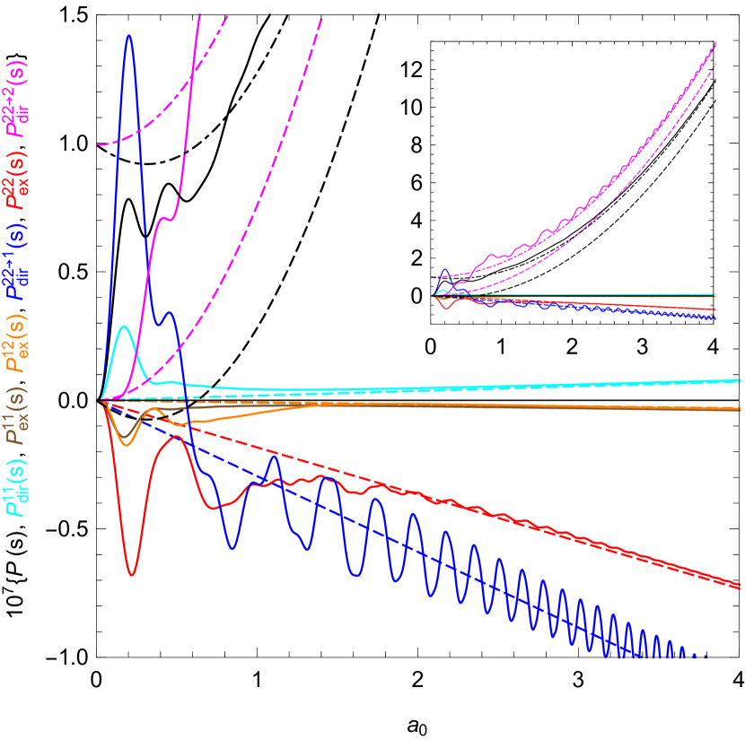
Figure 5: Dependence on $a_{0}$ for $s_{1}=s_{2}=s_{3}=1/3$, $\chi=1$ and $\mathcal{T}=\pi$.

Fig. 5 illustrates, for the short pulse, the transition form the one-step dominated regime to the two-step dominated one, by varying $a_{0}$ at fixed $\chi$ for a symmetric distribution of the lightfront momentum between the three particles. Notice, though, that for subunitary $a_{0}$, the comparison with LCF and, thus, the $\chi$ parameter lose their relevance. It is best to consider the dependence on $a_{0}$ at constant $b_{0}$. If $b_{0}$ is large, a small $\chi$ no longer implies an exponential suppression of the probability. While at large $a_{0}$ and constant $\chi$, $\mathbb{P}_{2}$ dominates $\mathbb{P}_{1}$ as $O\left(a_{0}^{2}\right)/O\left(a_{0}\right)$, at low $a_{0}$ and constant $b_{0}$ the opposite is true, as a direct Taylor expansion of the integrand shows that $\mathbb{P}_{2}\left(s\right)=O\left(a_{0}^{4}\right)$ and $\mathbb{P}_{1}\left(s\right)=O\left(a_{0}^{2}\right)$. Fig. 4 shows us, for the short pulse, how the two-step term loses importance compared to the one-step term, as $a_{0}$ decreases. All plots for a given $b_{0}$ have the same scale after dividing by $a_{0}^{2}$, so all the one-step curves and the one for the total result tend to a definite limit, while the two-step curve tends to zero, as $O(a_{0}^{2})$. Thus $\mathbb{P}\left(s\right)\approx a_{0}^{2}P^{0}\left(s\right)$ at low laser intensities. The limit $P^{0}\left(s\right)$ is independent of $a_{0}$. For a monochromatic field there is a threshold at $b_{0}=4$. For the pulse we consider here $P^{0}$ decays exponentially as $b_{0}<4$ decreases.

The $|\mathbb{P}_{1}\left(s\right)|/\mathbb{P}_{2}\left(s\right)$ ratio decreases not only with $a_{0}$, but also with pulse length. However, if the polarization is linear, the aforementioned oscillations make this decrease significantly slower for $\mathbb{P}_{\rm dir}^{22\rightarrow 1}\left(s\right)$ than for the other terms making up $\mathbb{P}_{1}\left(s\right)$. Only after one averages/integrates over $s$, they may become comparable. Pulse length also influences the validity of the aforementioned low $a_{0}$ expansions. The bigger it is, the smaller $a_{0}$ has to be for such perturbative expansions to work well. In fact, while an experimentalist’s biggest challenge may be to compress a pulse as much as possible, to make it both ultra-short and ultra-intense, the computational challenge is made higher by a longer, more diluted pulse of subunitary $a_{0}$, where all terms, two-step and one-step alike, are comparable and neither a perturbative nor an LCF approach can help.

The $\mathbb{P}_{\rm ex}^{22}\left(s\right)$ and $\mathbb{P}_{\rm dir}^{11}\left(s\right)$ terms are the closest to LCF, giving a decent order-of-magnitude estimate even at higher $b_{0}$ values where $\mathbb{P}_{\rm dir}^{22}$ is completely off the mark. A heuristic explanation is again related to the characteristic frequencies. For large $b_{0}$, $r_{1}/\left(2b_{0}\right)$ can be quite small in some relevant region, but is added to the larger $r_{2}/\left(2b_{0}\right)$ for $\mathbb{P}_{\rm dir}^{11}\left(s\right)\,$, while for $\mathbb{P}_{\rm ex}^{22}\left(s\right)$ there are larger frequency oscillations that couple all phase points $\phi_{i}$.

The interference terms $\mathbb{P}_{\rm ex}^{12}\left(s\right)$ and $\mathbb{P}_{\rm dir}^{12}\left(s\right)$ are seen to be relatively small for $a_{0}\geq 1$, but can be the same order of magnitude with the other terms for smaller $a_{0}$.

IV Numerical methods

To efficiently compute all terms that make up the exact (non-LCF) probability density $\mathbb{P}(s)$ we have used two different approaches, benchmarking one against the other when possible. The two classes of numerical methods have already been mentioned in Dinu:2017uoj , where, however, only class B was used and only to compute rates, not total probabilities. We now add to the B-type methods an ingredient to boost computation speed, which proves vital for the difficult $\mathbb{P}_{\rm ex}^{22}(s)$ term.

We give here a general description of the ideas behind the two classes of methods. In Appendix A we explain in detail the proper implementation of method $A$ for the most important terms. We stress the fact that, in talking about regularization, we do not mean the formulas from Dinu:2017uoj are not well defined as such, but only that, for practical computations, an infinitesimal epsilon is not convenient.

A. (${\rm A}_{1}$ and ${\rm A}_{2}$) This approach is well suited for computing all terms apart from $\mathbb{P}_{\rm ex}^{22}(s)$ and, in particular, it is vital for an efficient calculation of $\mathbb{P}_{\rm dir}^{22}(s)$ for realistic laser pulses, which have many oscillations. While being a bit involved, its complexity pays off greatly. The main idea is to change variables to the quantities $\Theta_{ij}$, whose linear combination appears in the exponent of the integrands, so as to reduce to a minimum the number of fast oscillating integrals and write the spectrum in the form of a linear combinations of Fourier transforms plus some residual terms involving lower dimension quadratures and special functions.

As already mentioned in Dinu:2017uoj the residual terms are computation-friendly analogues of half-free terms that involve interaction with the background field at just one of the two steps. They are due to the Heaviside functions originating in amplitude-level time ordering and do not occur in the two-step term $\mathbb{P}_{\rm dir}^{22\rightarrow 2}(s)$, where the domain of the $\Theta_{ij}$ integrals has been extended to the whole real axis, or in the lightfront instantaneous part $\mathbb{P}^{11}(s)$, where there is no step function.

For $\mathbb{P}_{\rm dir}^{22}(s)$, a manipulation of the Heaviside functions allows us to obtain triangular domains for the inner double quadrature in variables ($\phi_{1}$,$\phi_{3}$), which precedes the $(\Theta_{21},\Theta_{43})$ Fourier transforms, and have integrands made up of independent factors that can be sampled independently on a grid, thus keeping the numerical complexity of the ($\phi_{1}$,$\phi_{3}$) quadrature close to that required by just one single integral. Then, instead of performing the outer $(\Theta_{21},\Theta_{43})$ integrals as they are, the total phase of the complex exponential is used in method ${\rm A}_{1}$ as a new variable for a last, Fourier, integral, such that the quadrature that precedes it does not take oscillations from the complex exponential, so it is faster to perform. A specialized routine is used for the last integral, which only approximates the prefactor and uses exact integration of the resulting polynomial multiplied by trigonometric functions, so very frequent oscillations in the latter can accurately be followed without the need for a huge grid.

An even more efficient variant of this method that we will term ${\rm A}_{2}$, as opposed to the direct integration ${\rm A}_{1}$, involves computing intermediate interpolation tables. These are meant to store, for a given pulse shape and intensity, a table of partial derivatives of the inner integrals and then their Fourier transforms, which can be reused to quickly generate results for any combination of initial/final lightfront momenta ($b_{0}$ and $s$). To use an ordinary Fourier transform we take advantage of the fact that for the variable pair $\left(\Theta_{21},\Theta_{43}\right)$, too, the integration domain is triangular and that it can be brought to the upper half-plane by a 45 degree rotation. Moreover, the fact that an equally spaced rectangular grid in the new variables is a subset of a similar grid for the unrotated coordinates means we can produce the interpolation tables for the Fourier integrand efficiently by an independent sampling of the aforementioned factors and their derivatives in variables $\Theta_{21}$ and $\Theta_{43}$, too. All these reasons make it a very efficient method, well suited for computing results for long pulses, where ${\rm A}_{1}$ will be slow even for the computation of just a few points. The region covered by the tables has a limited extent, so an asymptotic expansion of the integrand outside them has to be performed and its integral can be computed analytically or by complex deformation for fast convergence.

B. This method uses regularization by deformation of the complex integrals into the complex plane, using the finite epsilon prescription described in Dinu:2017uoj . This is essential for $\mathbb{P}_{\rm ex}^{22}(s)$, for which the complexity of the formula and its singularities make regularization by either subtraction of simplified singular terms or partial integration rather unwieldy for practical purposes. Had the undeformed expression of $\mathbb{P}_{\rm ex}^{22}(s)$ (45) been regular or easy to make so, an A-type method involving changing variables to the total phase and thus limiting fast oscillations to only one integral would have been convenient.

At first sight, it seems that to produce even just one $\mathbb{P}_{\rm ex}^{22}(s)$ point, for a short pulse length, one needs a huge computing power. That is because the formula (45) involves four nested integrals, with long oscillating tails towards infinity, and the integrand itself has a complex formula.  When counting integrals we do not include the averages $\langle a\rangle$ and $\langle a^{2}\rangle$ which we pre-compute and tabulate for all terms and methods.

A great boost in speed can be obtained, for both exact and LCF results, by changing variables from $\phi_{i}\,\$(for probabilities) or $\theta_{ij}$ (coordinates relative to a given point, for rates) to one radial and some angular coordinates, depending on the dimensionality $d$ of the quadrature. Assuming the peak or center of the pulse is at the origin, we use polar coordinates for $\mathbb{P}^{11}(s)$ (39), spherical coordinates for $\mathbb{P}^{12}(s)$ (40), (41), given by

$$\phi_{1}=r\sin\theta\cos\beta\quad\phi_{2}=r\cos\theta\quad\phi_{3}=r\sin\theta\sin\beta$$ (8)

with $r\in[0,\infty)$, $\theta\in[0,\pi]$ and $\beta\in[\pi/4,5\pi/4]$, to implement time ordering, while for $\mathbb{P}_{\rm ex}^{22}(s)$ (45) we use a custom type of generalized spherical coordinates:

$$\begin{split}&\phi_{1}=r\cos\theta\cos\beta\quad\phi_{2}=r\sin\theta\cos\gamma\\ &\phi_{3}=r\cos\theta\sin\beta\quad\phi_{4}=r\sin\theta\sin\gamma\;,\end{split}$$ (9)

where $r\in\left[0,\infty\right)$, $\theta\in\left[0,\pi/2\right]$ and $\beta,\gamma\in\left[\pi/4,5\pi/4\right]$.

For computing the rate at a phase point $\phi$ a similar procedure is very useful, but using spherical coordinates relative to that point for $\mathcal{R}_{\rm ex}^{22}\left(s\right)$ and polar ones for $\mathcal{R}^{12}\left(s\right)$.

The factor $r^{d-1}$ in the Jacobian associated with this change amplifies the asymptotic oscillations and makes integrating to infinity unfeasible, in particular for $\mathbb{P}_{\rm ex}^{22}\left(s\right)$, where $d=4$. But, if one implements a cut-off in the radial direction and varies it, one sees that convergence of the total result within a very good precision is quickly reached. The reason is that if one first integrates on a hypersphere, at constant $r$, due to the many canceling oscillations on its surface, one obtains a result that decreases fast asymptotically, a thing unaffected by the $r^{d-1}$-proportional dilation of the hypersphere, as the density of the surface oscillations per unit solid angle also increases. After the integration over the radial direction and $\theta$ angular direction and with an appropriate choice of $\varepsilon$, the remaining angular integrals will have a limited amount of oscillations in them and few, if any, sign changes, which makes their computation efficient and accurate.

We want to limit the oscillations in the angular directions to a minimum and avoid small but fast canceling oscillations coming from the boundary of the ball, centered on the pulse, to which we restrict the integral. Therefore, instead of an abrupt cut-off at the boundary of the ball, we use a mollified one, multiplying the integrand by a $C^{\infty}$ function of $r$ that equals unity in this ball and slowly and smoothly goes to zero between it and a larger, concentric ball. In this way, convergence when varying the cut-off radius is faster and the computation time for a given radius is reduced.

We obtain a fast convergence even for small $\chi$ values, such as $1/2$, which are in the region of exponential suppression, unless only $a_{0}$ is small and not $b_{0}$. In this limit it is a greater challenge to compute the integral of what are initially fast oscillations, whose almost perfect cancelling brings the result down by several orders of magnitude, so the advantages of our method are even more apparent.

Especially for small $a_{0}$, it is very helpful to subtract from the integrand its free-field ($a_{0}=0$) counterpart, since the latter can be proven to yield a vanishing integral, as expected. We checked that in doing so the change in the result is negligible, providing another good test for our method.

We have also checked that, for $\mathbb{P}_{11}$ and $\mathbb{P}_{12}$, methods A and B give consistent results. We also checked that the exact and LCF trident rates, like the ones shown in Dinu:2017uoj , can be obtained more efficiently using spherical coordinates.

Outside the LCF approximation the rates are oscillating many times while slowly decaying outside the pulse, so it is preferable to apply method B directly to the probability terms. For LCF calculations the complex deformation introduces rapid decay at infinity, so the radial integrals are fast converging without any cut-off and the use of rates, tabulated in advance as function of $\chi$, is a good idea.

V Conclusions

We have studied the trident process in laser pulses with $a_{0}\gtrsim 1$, which mean that we have gone beyond the LCF approximation. We have found that for $a_{0}\gtrsim 1$ the (longitudinal) momentum spectrum has a richer structure compared to LCF. The corrections to the two-step, which we call one-step terms, are difficult to compute for long pulses, but they are anyway expected to be small for sufficiently long pulses. For shorter pulses they can be important though. We have studied all contributions for a short pulse, and found that the one-step terms can even become larger than the two-step for large electron momentum $b_{0}$. That the one-step can become dominant is expected from the perturbative limit, because only the one-step contributes to leading order $\mathcal{O}(a_{0}^{2})$. This is also consistent with the fact that the convergence to the LCF approximation needs larger $a_{0}$ for larger $b_{0}$.

For a field with longer pulse length we have explicitly demonstrated that, unless $b_{0}$ is large or $a_{0}$ small, the one-step terms become negligible and so the two-step can indeed be used to approximate the probability. This is evidence in support of using our new gluing approximation Dinu:2018efz ; gluingPaper for studying other higher-order processes in long laser pulses with moderately high intensity $a_{0}\gtrsim 1$.

Appendix A Numerical methods

Let us study the application of methods ${\rm A}_{1}$ and ${\rm A}_{2}$ to the integral $I$ appearing in the expression:

$$\mathbb{P}_{\rm dir}^{22}\left(s\right)=-\frac{\alpha^{2}}{4\pi^{2}b_{0}^{2}}\left[\frac{I}{q_{1}^{2}}+\left(1\leftrightarrow 2\right)\right]\;.$$ (10)

In order to make the changes of variables $\theta_{21}\rightarrow\Theta_{21}$, $\theta_{43}\rightarrow\Theta_{43}$ we notice the very useful fact that, since $\Theta_{ij}$ always grows with $\phi_{i}\,$ and decreases with $\phi_{j}$, we have the implications:

$$\begin{split}\left(\theta_{42}>0,~{}\Theta_{43}<\Theta_{21}\right)&\Rightarrow\theta_{31}>0\\ \left(\theta_{31}>0,~{}\Theta_{43}>\Theta_{21}\right)&\Rightarrow\theta_{42}>0\;,\end{split}$$ (11)

so we can express the time-ordering step functions as:

$$\begin{split}\theta\left(\theta_{42}\right)\theta\left(\theta_{31}\right)=&\theta\left(\theta_{42}\right)\theta\left(\Theta_{21}-\Theta_{43}\right)\\ &+\theta\left(\theta_{31}\right)\theta\left(\Theta_{43}-\Theta_{21}\right)\;.\end{split}$$ (12)

Therefore, we break the integral into two pieces, for which we choose the new variables to be $\left(\phi_{1},\Theta_{21},\phi_{3},\Theta_{43}\right)$ and $\left(\phi_{2},\Theta_{21},\phi_{4},\Theta_{43}\right)$, respectively. At first sight, the pieces are complex conjugates, so it seems we only have to compute the first one. The integration domain determined by the step functions is now triangular for both the pairs $\left(\phi_{1},\phi_{3}\right)$ and $\left(\Theta_{21},\Theta_{43}\right)$. Hence, we would like to be able to put the integral into the form:

$$I=\int\mathrm{d}\Theta_{21}\int_{\Theta_{21}}\mathrm{d}\Theta_{43}\int\mathrm{d}\phi_{1}\int_{\phi_{1}}\mathrm{d}\phi_{3}\operatorname{Re}J$$ (13)

We will however see later on that for some terms the two apparently complex conjugate integrals need to be kept separate and the way their boundary values extend to infinity must be correlated in a particular way, corresponding to a symmetric integration in the initial variables. To regularize the expression, i.e. be able to obtain a finite integrand $J$ without further need of the epsilon prescription, we keep in mind that $J$ is a linear combination of factorized terms of the form $F_{i}\left(\phi_{1},\Theta_{21};\omega_{1}\right)F_{j}\left(\phi_{3},\Theta_{43};\omega_{2}\right)$, where $\omega_{1}=\frac{r_{1}}{2b_{0}}$, $\omega_{2}=\frac{r_{2}}{2b_{0}}$,

$$F_{i}\left(\phi,\Theta;\omega\right)=f_{i}\left(\phi,\Theta\right)e^{i\omega\Theta}\;,$$ (14)

$$f_{0}=\tfrac{1}{\theta^{2}\left(\partial\Theta/\partial\theta\right)_{\phi}},~{}f_{1}=\tfrac{1}{\theta\left(\partial\Theta/\partial\theta\right)_{\phi}}\;,$$ (15)

and

$$\begin{split}&\left\{f_{2},f_{3},f_{4},f_{5}\right\}\\ &=\tfrac{\left\{\mathbf{w}_{1}\cdot\mathbf{w}_{2},w_{11}w_{22}-w_{12}w_{21},w_{11}w_{21}-w_{12}w_{22},w_{12}w_{21}+w_{11}w_{22}\right\}}{\theta\left(\partial\Theta/\partial\theta\right)_{\phi}}\;.\end{split}$$ (16)

Only $F_{0}$ and $F_{1}\,$are singular functions at $\Theta=0$, from whom we plan to subtract simpler, analytically integrable functions $F_{i}^{0}$ possessing the same singular part, using the decomposition

$$F_{i}F_{j}=G_{i}G_{j}+G_{i}F_{j}^{0}+F_{i}^{0}G_{j}+F_{i}^{0}F_{j}^{0}\;,$$ (17)

$$G_{i}=F_{i}-F_{i}^{0},$$ (18)

and making sure that the last term in 17 vanishes when integrated.

As explained in Dinu:2017uoj , doing this before the change of variables to $\Theta_{ij}$ and using for $F_{i}^{0}$ the free field $\left(a_{0}=0\right)$ version of $F_{i}$, provides an interpretation of the second and third terms in 17 as half-virtual, that is involving an interaction with the field at only one of the two steps. From a computational point of view, though, it is preferable to have only one Fourier exponential as a common factor, so as to regularize directly the pre-exponential factor. Hence we choose:

$$F_{i}^{0}=f_{i}^{0}e^{i\omega\Theta};~{}f_{0}^{0}=\tfrac{1}{\Theta^{2}};~{}f_{1}^{0}=\tfrac{1}{\Theta};~{}f_{i}^{0}=0,~{}i>1,$$ (19)

and write all formulas in terms of the regularized factors

$$g_{i}=f_{i}-f_{i}^{0}.$$ (20)

Successively plugging into the linear combination $J$ just one of the first three terms in 17 produces the decomposition:

$$I=I^{aa}+I^{a0}+I^{0a}\;.$$ (21)

We detail them below, starting with the first, four dimensional quadrature term:

$$I^{aa}=\operatorname{Re}\int\mathrm{d}\Theta_{21}\int_{\Theta_{21}}\mathrm{d}\Theta_{43}\left(A+iB\right)e^{i\left(\omega_{1}\Theta_{21}+\omega_{2}\Theta_{43}\right)}\;,$$ (22)

where

$$\begin{split}A&=T_{00}+\tfrac{\kappa_{01}}{2}T_{10}+\tfrac{\kappa_{23}}{2}T_{01}+\tfrac{\kappa_{01}}{2}\tfrac{\kappa_{23}}{2}\left(T_{11}+\tfrac{T_{22}}{\omega_{1}\omega_{2}}\right)\\ B&=\tfrac{\kappa_{01}}{2\omega_{1}}\left(T_{20}+\tfrac{\kappa_{23}}{2}T_{21}\right)+\tfrac{\kappa_{23}}{2\omega_{2}}\left(T_{02}+\tfrac{\kappa_{01}}{2}T_{12}\right)\end{split}$$ (23)

and $T_{ij}$ are obtained from double integrations which can be done efficiently, as they are defined on a triangular domain and the oscillations of the integrand only come from the pulse shape:

$$\begin{split}T_{00}&=-S_{11}-S_{44}-S_{55}\quad T_{10}=S_{61},~{}T_{01}=-S_{16}\\ T_{11}&=S_{66}+S_{33}\quad T_{22}=-S_{00}\quad T_{20}=-S_{01}\\ T_{21}&=-S_{06}\quad T_{02}=S_{10}\quad T_{12}=-S_{60}\;,\end{split}$$ (24)

where

$$S_{ij}=\int\mathrm{d}\phi_{1}\int_{\phi_{1}}\mathrm{d}\phi_{3}g_{i}\left(\phi_{1},\Theta_{21}\right)g_{j}\left(\phi_{3},\Theta_{43}\right)$$ (25)

and $g_{6}=g_{1}+g_{2}$.

A special routine was written for computing $S_{ij}$. For method ${\rm A}_{1}$ it first uses a preliminary adaptive Simpson method to sample the two functions  $g_{i}$ and $g_{j}$ on suitable nonuniform grids. Then follows a $\phi_{1}-$integration of the product of the piecewise polynomial approximations generated for $g_{i}\left(\phi_{1},\Theta_{21}\right)$ and $\int_{\phi_{1}}\mathrm{d}\phi_{3}g_{j}\left(\phi_{3},\Theta_{43}\right)$. In this way we only sample the two functions separately on a line, as for a one-dimensional integral. For method ${\rm A}_{2}$ each of the functions $g_{i}$ is accompanied in the above procedure by a few of its $\Theta_{ij}$ derivatives and, thus, a whole matrix of partial derivatives of $S_{ij}$ with respect to $(\Theta_{21},\Theta_{43})$ is produced. This is because method ${\rm A}_{1}$ is aimed at producing just one point value, while method ${\rm A}_{2}$ is meant to produce a whole set of spectra, for any $b_{0}$ and $(s_{1},s_{2})$ values.

For method ${\rm A}_{1}$ it is best to change variable to the exponent $\Theta=\omega_{1}\Theta_{21}+\omega_{2}\Theta_{43}$ and leave it for the last Fourier integral.

The procedure for ${\rm A}_{2}$ is more complex, as we want to create tables of values for 22 and we start by tabulating $T_{ij}$ together with a matrix of partial derivatives, obtained as described above. To turn the integration domain into the upper half-plane, we make a 45 degree rotation by changing the variables to $Z_{1}=\frac{\Theta_{43}+\Theta_{21}}{2}$ and $Z_{2}=\frac{\Theta_{43}-\Theta_{21}}{2}$. We then compute Fourier transforms with new frequencies $o_{1/2}=\omega_{1}\pm\omega_{2}$ for each element of the matrix of partial derivatives of each term $T_{ij}$ and a dense set of $o_{1}$ and $o_{2}$ values so as to create up to 9 interpolation tables, for general polarization.

The factor $1/q_{1}^{2}$ in 10 can ruin precision in the vicinity of $s_{1}=1$, but this can be avoided by a double partial integration, writing:

$$I^{aa}=-\frac{2}{o_{1}^{2}}\operatorname{Re}\int\mathrm{d}Z_{1}\int_{0}\mathrm{d}Z_{2}\left(\bar{A}+i\bar{B}\right)e^{i\left(o_{1}Z_{1}+o_{2}Z_{2}\right)}\;,$$ (26)

where $\bar{A}=\frac{\partial^{2}A}{\partial Z_{1}^{2}},~{}\bar{B}=\frac{\partial^{2}B}{\partial Z_{1}^{2}}$ are linear combinations of $\bar{T}_{ij}=\frac{\partial^{2}T_{ij}}{\partial Z_{1}^{2}}$. The replacement of $T_{ij}$ by $\bar{T}_{ij}$ means that, for a given maximum total order of the $Z$ partial derivatives, we now need to add two more orders in the tables that preceed the 45 degree rotations, whose elements are linear combinations of:

$$S_{ij}^{(pq)}=\int\mathrm{d}\phi_{1}\int_{\phi_{1}}\mathrm{d}\phi_{3}g_{i}^{\left(p\right)}\left(\phi_{1},\Theta_{21}\right)g_{j}^{\left(q\right)}\left(\phi_{3},\Theta_{43}\right),$$ (27)

where $g_{i}^{\left(p\right)}\left(\phi,\Theta\right)=\partial^{p}g_{i}\left(\phi,\Theta\right)/\partial\Theta^{p}$. We tabulate the set of partial derivatives on a grid with step $h$, so that $Z_{1}=j_{1}h$, $Z_{2}=j_{2}h$, $j_{2}\geq 0$ hence $\Theta_{43}=i_{1}h,~{}\Theta_{21}=i_{2}h$ and $i_{1/2}=j_{1}\pm j_{2}$. This can be done highly efficiently in the following manner:

In order to reduce memory storage, we concentrate at one time on just one small piece of the $\phi_{1}$ integrals, covering an interval of length $l$, adding to the contribution of the previous intervals. Say we use derivatives up to order 4. For a grid of $i_{1}$ and $i_{2}$ values we determine, using an adaptive Simpson method, piecewise polynomial approximations for $g_{i}^{\left(p\right)}\left(\phi_{1},\Theta_{21}\right)$ and $\int_{\phi_{1}}\mathrm{d}\phi_{3}g_{j}^{\left(q\right)}\left(\phi_{3},\Theta_{43}\right)$ on two different grids of $\phi_{1}$ values, for $p,q=0,1,...,6$ and for a square $n\times n$ matrix of $\left(\Theta_{21},\Theta_{43}\right)$ values, which cover only a small square part of the domain we want covered.

If $n$ is large enough, the computation of the functions and derivatives, the adaptive Simpson procedure and the subsequent sorting of the grid points cost little compared to the $n^{2}$ $\phi_{1}$ integrals that are performed, using a custom integration tool for the product of piecewise polynomial interpolations. Then the procedure is repeated for all relevant $\phi_{1}$ intervals and, after implementing the rotation, we save to an external memory the values of $\bar{T}_{ij}$ and its derivatives on a square matrix of equally spaced $\left(Z_{1},Z_{2}\right)$ values, one out of many that are to be computed and stored for the next step. If the grid spacing$\ h$ is small enough, by a Taylor expansion, we can find with good precision $\bar{T}_{ij}$ at any point inside the square block where the $\left(Z_{1},Z_{2}\right)$ values lie.

The second step involves a custom code for implementing the double Fourier transform, using, for each $h$ interval centered at a grid point, analytical formulas for the integral of an oscillating exponential multiplied by the aforementioned Taylor series. Since we cannot compute an infinite number of blocks, we cover a finite rectangle with these blocks and use for $\bar{T}_{ij}$ an asymptotic extrapolation as a polynomial decay times oscillation, which can be used to extend the integration to infinity, with good approximation. In this asymptotic region the integral can be expressed in terms of trigonometric integrals, or a complex rotation of the integration path may be used to turn the oscillating exponential into a decaying one.

The double Fourier transform of each $\bar{T}_{ij}$ is computed and stored as a table for a dense set of $o_{1}$, $o_{2}$ values, with $\left|o_{2}\right|<o_{1}<o_{\max}$, where the $o_{\max}$ is chosen large enough to provide all the nonnegligible part of the spectrum for the minimum $\chi$ value we have in mind. Then, for any $b_{0}$ and $s$ values, $I^{aa}$ is produced from interpolations of the data in the tables. Next we describe the residual terms, choosing $I^{a0}$ for more detailed explanations.

Let $\tilde{g}_{i}$ be the function obtained from $g_{i}$ by replacing $\phi_{1}$ by $\phi_{2}$ as variable independent of $\Theta_{21}$.

$$\begin{split}I^{a0}=&\int\mathrm{d}\Theta_{21}\int_{\Theta_{21}}\mathrm{d}\Theta_{43}\int\mathrm{d}\phi_{1}\int_{\phi_{1}}^{L_{1}\rightarrow\infty}\mathrm{d}\phi_{3}\left(\frac{-id_{0}}{\Theta_{43}^{2}}+\frac{d_{1}}{\Theta_{43}}\right)e^{i\omega_{2}\Theta_{43}}\\ &\times\left(ic_{0}g_{0}\left(\phi_{1},\Theta_{21}\right)+c_{1}g_{1}\left(\phi_{1},\Theta_{21}\right)+c_{2}g_{2}\left(\phi_{1},\Theta_{21}\right)\right)e^{i\omega_{1}\Theta_{21}}\\ &+\int\mathrm{d}\Theta_{21}\int^{\Theta_{21}}\mathrm{d}\Theta_{43}\int\mathrm{d}\phi_{2}\int_{\phi_{2}}^{L_{2}\rightarrow\infty}\mathrm{d}\phi_{4}\left(\frac{-id_{0}}{\Theta_{43}^{2}}+\frac{d_{1}}{\Theta_{43}}\right)e^{i\omega_{2}\Theta_{43}}\\ &\times\left(ic_{0}\tilde{g}_{0}\left(\phi_{2},\Theta_{21}\right)+c_{1}\tilde{g}_{1}\left(\phi_{2},\Theta_{21}\right)+c_{2}\tilde{g}_{2}\left(\phi_{2},\Theta_{21}\right)\right)e^{i\omega_{1}\Theta_{21}}\;,\end{split}$$ (28)

where $c_{2}=\frac{\kappa_{01}}{2}$, $c_{1}=c_{2}-1$, $c_{0}=-\frac{2b_{0}}{r_{1}}c_{2}$, $d_{2}=\frac{\kappa_{23}}{2}$, $d_{0}=-\frac{2b_{0}}{r_{2}}d_{2}$, and $d_{1}=d_{2}+1$.

We have to write the expression like this, before going to just one integral like in 13, for an essential ingredient is finding out how $L_{1}$ and $L_{2}$ are to be related for a symmetric integration around the average phase $\sigma_{ij}$, instead of a discontinuous choice of the variables that are independent from $\Theta_{ij}$. By breaking the integration domain into two parts, each with a different definition of the variables independent of $\left(\Theta_{21},\Theta_{43}\right)$, we effectively severed the $\Theta_{21}$ and $\Theta_{43}$ integrals and reattached them with a displacement, which has to be taken into account. Hence we cannot just keep $L_{1}$ and $L_{2}$ equal as they tend to infinity, for this would give a value for the probability that can even be negative at low $a_{0}$. Instead, since for a fixed $\Theta_{43}$ value, at large $\phi$, $\Theta_{43}=\theta_{43}$, to keep the integration symmetric, we should choose $L_{1}=L-\Theta_{43}/2,~{}L_{2}=L+\Theta_{43}/2$, with $L\rightarrow\infty$. We have checked that this A-type method gives the same results as what we obtain by integrating the rates in Dinu:2017uoj , which were obtained with a B-type method.

We introduce the following special functions:

$$\begin{split}W\left(x\right)&=\int_{-\infty}^{x}\!\mathrm{d}y\frac{\exp\left(iy\right)}{y+i\varepsilon}\rightarrow\operatorname{Ei}\left(ix\right)-i\pi\operatorname*{sgn}\left(x\right),\end{split}$$ (29)

$$\begin{split}W_{2}\left(x\right)=\int_{-\infty}^{x}\!\mathrm{d}y\frac{\exp\left(iy\right)}{\left(y+i\varepsilon\right)^{2}}\rightarrow iW\left(x\right)-\frac{e^{ix}}{x}.\end{split}$$ (30)

We use the above integrals, then in the second term we swap the two indices of $\Theta_{21}$, after which we change the sign of $\Theta_{21}$ to keep the same exponent.

$$\begin{split}2I^{a0}=&\int\mathrm{d}\Theta_{21}\int\mathrm{d}\phi_{1}\left[\left(\phi_{1}-L\right)\left(d_{1}W\left(\omega_{2}\Theta_{21}\right)-id_{0}\omega_{2}W_{2}\left(\omega_{2}\Theta_{21}\right)\right)+\frac{1}{2}\left(\frac{d_{1}e^{i\omega_{2}\Theta_{21}}}{i\omega_{2}}-id_{0}W\left(\omega_{2}\Theta_{21}\right)\right)\right]\\ &\times\left(-ic_{0}g_{0}\left(\phi_{1},\Theta_{21}\right)+c_{1}g_{1}\left(\phi_{1},\Theta_{21}\right)+c_{2}g_{2}\left(\phi_{1},\Theta_{21}\right)\right)e^{i\omega_{1}\Theta_{21}}\\ &+\int\mathrm{d}\Theta_{21}\int\mathrm{d}\phi_{1}\left[\left(L-\phi_{1}\right)\left(d_{1}W\left(\omega_{2}\Theta_{21}\right)-id_{0}\omega_{2}W_{2}\left(\omega_{2}\Theta_{21}\right)\right)+\frac{1}{2}\left(\frac{d_{1}e^{i\omega_{2}\Theta_{21}}}{i\omega_{2}}-id_{0}W\left(\omega_{2}\Theta_{21}\right)\right)\right]\\ &\times\left(-ic_{0}\tilde{g}_{0}\left(\phi_{1},\Theta_{21}\right)+c_{1}\tilde{g}_{1}\left(\phi_{1},\Theta_{21}\right)+c_{2}\tilde{g}_{2}\left(\phi_{1},\Theta_{21}\right)\right)e^{i\omega_{1}\Theta_{21}}\end{split}$$ (31)

We now use the symmetric role of the two $\phi$ values, which implies that $\tilde{g}_{0}\left(\phi_{1},\Theta_{21}\right)=g_{0}\left(\phi_{1},-\Theta_{21}\right)$ and $\tilde{g}_{i}\left(\phi_{1},\Theta_{21}\right)=-g_{i}\left(\phi_{1},-\Theta_{21}\right)$, $i\neq 0$.

Using the notation $W_{0}\left(x\right)=W\left(x\right)e^{-ix}$ for what is a non-oscillating function, easy to be produced from an interpolation table and series expansions near the origin and at large values, we obtain the final formulas for the residual terms:

$$\begin{split}I^{a0}&=\operatorname{Re}\int_{0}\mathrm{d}\Theta\exp\left(i\omega\Theta\right)\left[W_{0}\left(\omega_{2}\Theta\right)+\tfrac{id_{0}}{\Theta}\right]\left[c_{1}G_{1}+c_{2}G_{2}-ic_{0}G_{0}\right]\\ &+\operatorname{Im}\int_{0}\mathrm{d}\Theta\exp\left(i\omega\Theta\right)\left[\tfrac{d_{1}}{\omega_{2}}+d_{0}W_{0}\left(\omega_{2}\Theta\right)\right]\left[c_{1}\check{G}_{1}+c_{2}\check{G}_{2}-ic_{0}\check{G}_{0}\right]\;,\end{split}$$ (32)

$$\begin{split}I^{0a}&=\operatorname{Re}\int_{0}\mathrm{d}\Theta\exp\left(i\omega\Theta\right)\left[-W_{0}\left(\omega_{1}\Theta\right)+\tfrac{ic_{0}}{\Theta}\right]\left[d_{1}G_{1}+d_{2}G_{2}-id_{0}G_{0}\right]\\ &+\operatorname{Im}\int_{0}\mathrm{d}\Theta\exp\left(i\omega\Theta\right)\left[\tfrac{c_{1}}{\omega_{1}}+c_{0}W_{0}\left(\omega_{1}\Theta\right)\right]\left[d_{1}\check{G}_{1}+d_{2}\check{G}_{2}-id_{0}\check{G}_{0}\right]\;,\end{split}$$ (33)

where $G_{i}=\int\phi\bar{g}_{i}\left(\phi,\Theta\right)\mathrm{d}\phi,~{}\check{G}_{i}=\int\check{g}_{i}\left(\phi,\Theta\right)\mathrm{d}\phi$ and $\bar{g}_{0}\left(\phi,\Theta\right)\equiv g_{0}\left(\phi,\Theta\right)-g_{0}\left(\phi,-\Theta\right)$, $\bar{g}_{i}\left(\phi,\Theta\right)\equiv g_{i}\left(\phi,\Theta\right)+g_{i}\left(\phi,-\Theta\right)$ for $i\neq 0$, $\check{g}_{0}\left(\phi,\Theta\right)\equiv\frac{g_{0}\left(\phi,\Theta\right)+g_{0}\left(\phi,-\Theta\right)}{2}$, $\check{g}_{i}\left(\phi,\Theta\right)\equiv\frac{g_{i}\left(\phi,\Theta\right)-g_{i}\left(\phi,-\Theta\right)}{2}$ for $i\neq 0$. We have checked analytically that for $a_{0}\ll 1$ we find agreement between $I^{0a}$ and the high-energy limit of perturbative $\mathcal{O}(a_{0}^{2})$ trident. Since both the Re… and Im… terms in $I^{0a}$ contribute to leading order, this is a nontrivial check of the choice of the boundaries $L_{1}$ and $L_{2}$ above.

Similarly to what has already been described before, method ${\rm A}_{1}$ uses direct integration, while method ${\rm A}_{2}$ involves the tabulation of the functions $G_{i}$,$~{}\check{G}_{i}$ and a few of their derivatives, for a large region of $\Theta$ values, so as to be used repeatedly to compute the integrals for any $b_{0}$ and $s_{i}$ values. Here, too, a double integration by parts is very useful to prevent precision loss. We can extend the tables enough as to not need asymptotic expansions, as convergence is fast enough.

Next we want to calculate (40) and (41):

$$\mathbb{P}_{\rm dir/ex}^{12}\left(s\right)=\frac{\alpha^{2}}{4\pi^{2}b_{0}}\left[I_{\rm dir/ex}^{12}+\left(1\leftrightarrow 2\right)\right]$$ (34)

To make the formulas very similar to the ones before, we interchange even and odd indices, so $\phi_{1}\leftrightarrow\phi_{2}$, $\phi_{3}\rightarrow\phi_{4}$ and the three phase points are $\phi_{1},\phi_{2},\phi_{4}$. The direct term needs no regularization and, therefore, it has no residual terms, $I_{\rm dir}^{12}=I_{\rm dir}^{12aa}$, while the exchange one has the decomposition $I_{\rm ex}=I_{\rm ex}^{12aa}+I_{\rm ex}^{12a0}+I_{\rm ex}^{120a}$

$$\begin{split}I_{\rm dir/ex}^{12aa}=\int\mathrm{d}\Theta_{21}\int_{\Theta_{21}}\mathrm{d}\Theta_{41}B_{\rm dir/ex}^{12}\sin\left(\omega_{1}\Theta_{21}+\omega_{2}\Theta_{41}\right)\;,\end{split}$$ (35)

$$B_{\rm dir}^{12}=\frac{\left(1+s_{1}\right)\left(s_{2}-s_{3}\right)}{q_{1}^{3}}\int\mathrm{d}\phi_{1}\mathbf{g}_{a}\left(\phi_{1},\Theta_{21}\right)\cdot\mathbf{g}_{a}\left(\phi_{1},\Theta_{41}\right)\;,$$ (36)

$$\begin{split}B_{\rm ex}^{12}&=\int\mathrm{d}\phi_{1}\bigg{[}-\tfrac{q_{1}}{q_{2}^{2}}g_{1}\left(\phi_{1},\Theta_{21}\right)g_{1}\left(\phi_{1},\Theta_{41}\right)\\ &\hskip 28.45274pt+\tfrac{s_{1}s_{3}-s_{2}}{q_{1}q_{2}^{2}}\mathbf{g}_{a}\left(\phi_{1},\Theta_{21}\right)\cdot\mathbf{g}_{a}\left(\phi_{1},\Theta_{41}\right)\bigg{]}\;,\end{split}$$ (37)

where $\mathbf{g}_{a}\left(\phi,\Theta\right)=\tfrac{\mathbf{w}_{2}/\theta}{\left(\partial\Theta/\partial\theta\right)_{\phi}}$, and

$$\begin{split}I_{\rm ex}^{12a0}+I_{\rm ex}^{120a}=-2\tfrac{q_{1}}{q_{2}^{2}}\operatorname{Im}\int_{0}&\mathrm{d}\Theta\exp\left(i\omega\Theta\right)\check{G}_{1}\left(\Theta\right)\\ \times&\left[W_{0}\left(\omega_{1}\Theta\right)-W_{0}\left(\omega_{2}\Theta\right)\right]\;.\end{split}$$ (38)

Notice that all residual terms vanish in the LCF approximation, but they can be essential at low $a_{0}$/large $b_{0}$, where they dominate.

The procedure to compute just the two-step term, $\mathbb{P}_{\rm dir}^{22\rightarrow 2}(s)$, is similar to the one for $\mathbb{P}_{\rm dir}^{22}(s)$, except that we use the average coordinates $\sigma_{21}=\frac{\phi_{1}+\phi_{2}}{2}$ and $\sigma_{43}=\frac{\phi_{3}+\phi_{4}}{2}$ as independent variables and there are no residual terms. We will not present the details, as they are easy to infer, but mention that we need only up to five tables here, for general polarization, if we make the partial integration used in Eqs. (34)-(37) in Dinu:2017uoj . Again, a double partial integration can bring out a factor of $\omega_{2}^{-2}$, to mitigate the singularity $q_{1}^{-2}$ present in the formula when $s_{1}$ is close to unity. Asymptotic expansions outside the region covered by the tables are essential for the two-step terms, which have slower asymptotic decay than for the integrals encountered before and even more important for the LCF approximation to the two-step probability that can also be computed by the same method. To compute $\mathbb{P}^{11}\left(s\right)$ we need similar interpolation tables for the Fourier integrand and its transform, but these are one-dimensional, so require fewer resources. Here, too, the integrand is approximated by an expansion outside the tables.

Appendix B Formulas

For the readers’ convenience we collect the formulas from Dinu:2017uoj in this appendix. The total probability is given by the sum of the following 6 terms:

$$\{\mathbb{P}_{\rm dir}^{11}(s),\mathbb{P}_{\rm ex}^{11}(s)\}=\frac{\alpha^{2}}{\pi^{2}}\int\!\mathrm{d}\phi_{12}\left\{\frac{1}{q_{1}^{4}}+\frac{1}{q_{2}^{4}},-\frac{1}{q_{1}^{2}q_{2}^{2}}\right\}\frac{-s_{0}s_{1}s_{2}s_{3}}{(\theta_{21}+i\epsilon)^{2}}\exp\left\{\frac{i}{2b_{0}}(r_{1}+r_{2})\Theta_{21}\right\}\;,$$ (39)

$$\mathbb{P}_{\rm dir}^{12}(s)=\text{Re }i\frac{\alpha^{2}}{4\pi^{2}b_{0}}\int\!\mathrm{d}\phi_{123}\theta(\theta_{31})\frac{(s_{0}+s_{1})(s_{2}-s_{3})D_{12}}{q_{1}^{3}(\theta_{21}+i\epsilon)(\theta_{23}+i\epsilon)}\exp\left\{\frac{i}{2b_{0}}\left[r_{1}\Theta_{21}+r_{2}\Theta_{23}\right]\right\}+(s_{1}\leftrightarrow s_{2})\;,$$ (40)

$$\mathbb{P}_{\rm ex}^{12}(s)=\text{Re}\frac{-i\alpha^{2}}{4\pi^{2}b_{0}}\int\!\mathrm{d}\phi_{123}\theta(\theta_{31})\frac{q_{1}^{2}+[s_{0}s_{2}-s_{1}s_{3}]D_{12}}{q_{1}q_{2}^{2}(\theta_{21}+i\epsilon)(\theta_{23}+i\epsilon)}\exp\left\{\frac{i}{2b_{0}}\left[r_{1}\Theta_{21}+r_{2}\Theta_{23}\right]\right\}+(s_{1}\leftrightarrow s_{2})\;,$$ (41)

$$\begin{split}\mathbb{P}_{\rm dir}^{22}(s)=-\frac{\alpha^{2}}{8\pi^{2}b_{0}^{2}}&\int\!\mathrm{d}\phi_{1234}\frac{\theta(\theta_{31})\theta(\theta_{42})}{q_{1}^{2}\theta_{21}\theta_{43}}\exp\left\{\frac{i}{2b_{0}}\left(r_{1}\Theta_{21}+r_{2}\Theta_{43}\right)\right\}\left\{\frac{\kappa_{01}\kappa_{23}}{4}W_{1234}+W_{1324}+W_{1423}\right.\\ &\left.+\left[\frac{\kappa_{01}}{2}\left(\frac{2ib_{0}}{r_{1}\theta_{21}}+1+D_{1}\right)-1\right]\left[\frac{\kappa_{23}}{2}\left(\frac{2ib_{0}}{r_{2}\theta_{43}}+1+D_{2}\right)+1\right]-D_{1}D_{2}\right\}+(s_{1}\leftrightarrow s_{2})\;,\end{split}$$ (42)

where $\theta_{ij}=\phi_{i}-\phi_{j}$, $\mathrm{d}\phi_{1234}=\mathrm{d}\phi_{1}...\mathrm{d}\phi_{4}$, $r_{1}=(1/s_{1})-(1/s_{0})$, $r_{2}=(1/s_{2})+(1/s_{3})$, $\kappa_{ij}=(s_{i}/s_{j})+(s_{j}/s_{i})$, $\Theta_{ij}:=\theta_{ij}M^{2}_{ij}$, the effective mass Kibble:1975vz $M^{2}=1+\langle a_{\scriptscriptstyle\perp}^{2}\rangle-\langle a_{\scriptscriptstyle\perp}\rangle^{2}$, $\langle a\rangle=\frac{1}{\theta}\int_{\phi_{1}}^{\phi_{2}}a$, $D_{12}={\bf\Delta}_{12}\!\cdot\!{\bf\Delta}_{32}$ and

$$W_{ijkl}:=(\mathbf{w}_{i}\!\times\!\mathbf{w}_{j})\!\cdot\!(\mathbf{w}_{k}\!\times\!\mathbf{w}_{l})=(\mathbf{w}_{i}\!\cdot\!\mathbf{w}_{k})(\mathbf{w}_{j}\!\cdot\!\mathbf{w}_{l})-(\mathbf{w}_{i}\!\cdot\!\mathbf{w}_{l})(\mathbf{w}_{j}\!\cdot\!\mathbf{w}_{k})\;,$$ (43)

which we separate into $\mathbb{P}_{\rm dir}^{22}=\mathbb{P}_{\rm dir}^{22\to 2}+\mathbb{P}_{\rm dir}^{22\to 1}$, where $\mathbb{P}_{\rm dir}^{22\to 2}$ and $\mathbb{P}_{\rm dir}^{22\to 1}$ are obtained by replacing $\theta(\theta_{31})\theta(\theta_{42})$ with the first and second term in

$$\theta(\theta_{42})\theta(\theta_{31})=\theta(\sigma_{43}-\sigma_{21})\left\{1-\theta\left(\frac{|\theta_{43}-\theta_{21}|}{2}-[\sigma_{43}-\sigma_{21}]\right)\right\}\;,$$ (44)

respectively, and

$$\begin{split}\mathbb{P}_{\rm ex}^{22}(s)=\text{Re}\frac{\alpha^{2}}{16\pi^{2}b_{0}^{2}}&\int\!\mathrm{d}\phi_{1234}\frac{\theta(\theta_{42})\theta(\theta_{31})}{s_{0}s_{1}s_{2}s_{3}d_{0}}\Bigg{\{}F_{0}+f_{0}-\frac{2ib_{0}}{d_{0}}(f_{1}+z_{1})+\left[\frac{2b_{0}}{d_{0}}\right]^{2}z_{2}\Bigg{\}}\\ &\exp\left\{\frac{i}{2b_{0}}\frac{q_{1}q_{2}}{s_{0}s_{1}s_{2}s_{3}d_{0}}\left(\theta_{41}\theta_{23}\left[\frac{\Theta_{41}}{s_{1}}+\frac{\Theta_{23}}{s_{2}}\right]+\theta_{43}\theta_{21}\left[\frac{\Theta_{43}}{s_{3}}-\frac{\Theta_{21}}{s_{0}}\right]+\theta_{31}\theta_{42}\left[\frac{\Theta_{31}}{q_{2}}-\frac{\Theta_{42}}{q_{1}}\right]\right)\right\}\;.\end{split}$$ (45)

The prefactor of (45) can be expressed in terms of a permutation defined by

$${\sf P}[\mathcal{F}]:=\mathcal{F}(\phi_{1}\to\phi_{2}\to\phi_{3}\to\phi_{4}\to\phi_{1},s_{1}\to-s_{0}\to s_{2}\to s_{3}\to s_{1})\;,$$ (46)

as

$${\bf d}_{1}=\frac{1}{d_{0}}\left(\frac{\theta_{23}}{s_{2}}\frac{\theta_{41}}{s_{1}}{\bf\Delta}_{14}+\frac{\theta_{21}}{s_{0}}\frac{\theta_{43}}{s_{3}}{\bf\Delta}_{12}+\frac{\theta_{42}\theta_{23}}{s_{2}s_{3}}[{\bf\Delta}_{24}-{\bf\Delta}_{23}]\right)\qquad d_{0}=\frac{\theta_{23}}{s_{2}}\frac{\theta_{41}}{s_{1}}+\frac{\theta_{21}}{s_{0}}\frac{\theta_{43}}{s_{3}}\;,$$ (47)

$${\bf d}_{2}={\sf P}[{\bf d}_{1}]\qquad{\bf d}_{3}={\sf P}[{\bf d}_{2}]\qquad{\bf d}_{4}={\sf P}[{\bf d}_{3}]\qquad{\bf d}_{1}={\sf P}[{\bf d}_{4}]\;.$$ (48)

$$F_{0}=(1+{\sf P})\kappa_{03}[({\bf d}_{1}\!\cdot\!{\bf d}_{3})({\bf d}_{2}\!\cdot\!{\bf d}_{4})+(\mathbf{d}_{1}\!\times\!\mathbf{d}_{3})\!\cdot\!(\mathbf{d}_{2}\!\times\!\mathbf{d}_{4})]\;,$$ (49)

$$\begin{split}f_{0}&=(1+{\sf P})\frac{1}{s_{0}s_{1}s_{2}s_{3}}(s_{1}q_{2}{\bf d}_{1}-s_{2}q_{1}{\bf d}_{2})\!\cdot\!(s_{2}q_{2}{\bf d}_{3}-s_{1}q_{1}{\bf d}_{4})\;,\\ f_{1}&=-(1+{\sf P}+{\sf P}^{2}+{\sf P}^{3})\kappa_{03}\frac{\theta_{21}}{s_{0}}{\bf d}_{2}\!\cdot\!{\bf d}_{1}+(1+{\sf P})(\kappa_{03}-\kappa_{12})\frac{\theta_{42}}{q_{1}}{\bf d}_{4}\!\cdot\!{\bf d}_{2}\;,\end{split}$$ (50)

$$z_{1}=(1+{\sf P}+{\sf P}^{2}+{\sf P}^{3})\frac{-q_{1}^{2}}{s_{0}s_{1}q_{2}}\left(3+\frac{s_{2}s_{3}}{s_{0}s_{1}}\right)\phi_{1}\qquad z_{2}=(1+{\sf P})\kappa_{03}\left(\frac{\theta_{43}}{s_{3}}\frac{\theta_{21}}{s_{0}}+\frac{\theta_{31}}{q_{2}}\frac{\theta_{42}}{q_{1}}\right)\;.$$ (51)

We have obtained these results by performing the Gaussian integrals over $p_{1{\scriptscriptstyle\perp}}$ and $p_{2{\scriptscriptstyle\perp}}$. For the direct terms we find that the Gaussian peak is located at

$$p_{1}^{\scriptscriptstyle\perp}=\langle a\rangle_{21}^{\scriptscriptstyle\perp}+s_{1}(p^{\scriptscriptstyle\perp}-\langle a\rangle_{21}^{\scriptscriptstyle\perp})$$ (52)

and

$$p_{2}^{\scriptscriptstyle\perp}=\langle a\rangle_{43}^{\scriptscriptstyle\perp}+s_{2}(p^{\scriptscriptstyle\perp}-\langle a\rangle_{21}^{\scriptscriptstyle\perp})\;,$$ (53)

which means

$$p_{3}^{\scriptscriptstyle\perp}=-\langle a\rangle_{43}^{\scriptscriptstyle\perp}+s_{3}(p^{\scriptscriptstyle\perp}-\langle a\rangle_{21}^{\scriptscriptstyle\perp})\;.$$ (54)

It is experimentally relevant to assume that $\gamma=p_{0}$ is much larger than all the other parameters, and then we have to leading order

$${\bf p}_{i}\approx s_{i}{\bf p}\;.$$ (55)

The peak for the exchange terms is in general more complicated, but reduces (55) to leading order. Thus, in this regime all particles in the final state have momenta approximately parallel to the initial momentum. $s_{i}$ is by definition the fraction of the initial longitudinal momentum given to particle $i$. From (55) we see that it also gives the fraction of the total momentum to leading order. $s_{i}$ are therefore natural variables to focus on. After shifting and diagonalizing the transverse momentum variables, the exponential becomes $e^{-c_{1}p_{1{\scriptscriptstyle\perp}}^{2}-c_{2}p_{2{\scriptscriptstyle\perp}}^{2}}$. The coefficients $c_{1}$ and $c_{2}$ determine the width of the Gaussian peak. $c_{i}$ can be expressed in terms of $s_{i}$ and $\phi_{i}$ and scale with $a_{0}$ and $b_{0}$, but do depend on $\gamma$ separately ($b_{0}$ is much smaller than $\gamma$). The width of the Gaussian peak is therefore much smaller than its position.

References

- (1) V. Dinu and G. Torgrimsson, “Trident pair production in plane waves: Coherence, exchange, and spacetime inhomogeneity,” Phys. Rev. D 97, no. 3, 036021 (2018) [arXiv:1711.04344 [hep-ph]].
- (2) B. King and A. M. Fedotov, “Effect of interference on the trident process in a constant crossed field,” Phys. Rev. D 98, no. 1, 016005 (2018) [arXiv:1801.07300 [hep-ph]].
- (3) F. Mackenroth and A. Di Piazza, “Nonlinear trident pair production in an arbitrary plane wave: a focus on the properties of the transition amplitude,” Phys. Rev. D 98, no. 11, 116002 (2018) [arXiv:1805.01731 [hep-ph]].
- (4) U. Hernandez Acosta and B. Kämpfer, “Laser pulse-length effects in trident pair production,” Plasma Phys. Control. Fusion 61, no. 8, 084011 (2019) [arXiv:1901.08860 [hep-ph]].
- (5) K. Krajewska and J. Z. Kamiński, “Circular dichroism in nonlinear electron-positron pair creation”, Journal of Physics: Conference Series 594 012024 (2015)
- (6) H. Hu and J. Huang, “Trident pair production in colliding bright x-ray laser beams,” Phys. Rev. A 89 (2014) no.3, 033411 [arXiv:1308.5324 [physics.atom-ph]].
- (7) B. King and H. Ruhl, “Trident pair production in a constant crossed field,” Phys. Rev. D 88, no. 1, 013005 (2013) [arXiv:1303.1356 [hep-ph]].
- (8) A. Ilderton, “Trident pair production in strong laser pulses,” Phys. Rev. Lett. 106, 020404 (2011) [arXiv:1011.4072 [hep-ph]].
- (9) H. Hu, C. Muller and C. H. Keitel, “Complete QED theory of multiphoton trident pair production in strong laser fields,” Phys. Rev. Lett. 105, 080401 (2010) [arXiv:1002.2596 [physics.atom-ph]].
- (10) C. Bamber et al., “Studies of nonlinear QED in collisions of 46.6-GeV electrons with intense laser pulses,” Phys. Rev. D 60, 092004 (1999).
- (11) V. N. Baier, V. M. Katkov, and V. M. Strakhovenko, Soviet Phys. Nucl. Phys 14, 572 (1972).
- (12) V. I. Ritus, “Vacuum polarization correction to elastic electron and muon scattering in an intense field and pair electro- and muoproduction,” Nucl. Phys. B 44 (1972) 236.
- (13) J. Esberg et al. [CERN NA63 Collaboration], “Experimental investigation of strong field trident production,” Phys. Rev. D 82, 072002 (2010).
- (14) “Probing strong-field QED in electron-photon interactions”, 21-24 August 2018, DESY https://indico.desy.de/indico/event/19493/overview
- (15) Presentation by A. Hartin at DESY https://indico.desy.de/indico/event/19510/
- (16) H. Abramowicz et al., “Letter of Intent for the LUXE Experiment,” arXiv:1909.00860 [physics.ins-det].
- (17) Presentation by S. Meuren, “Probing Strong-field QED at FACET-II (SLAC E-320)”, Stanford. https://conf.slac.stanford.edu/facet-2-2019/sites/facet-2-2019.conf.slac.stanford.edu/files/basic-page-docs/sfqed_2019.pdf
- (18) A. R. Bell and J. G. Kirk, “Possibility of Prolific Pair Production with High-Power Lasers,” Phys. Rev. Lett. 101, 200403 (2008).
- (19) N. V. Elkina, A. M. Fedotov, I. Y. Kostyukov, M. V. Legkov, N. B. Narozhny, E. N. Nerush and H. Ruhl, “QED cascades induced by circularly polarized laser fields,” Phys. Rev. ST Accel. Beams 14, 054401 (2011) [arXiv:1010.4528 [hep-ph]].
- (20) E. N. Nerush, I. Y. Kostyukov, A. M. Fedotov, N. B. Narozhny, N. V. Elkina and H. Ruhl, “Laser field absorption in self-generated electron-positron pair plasma,” Phys. Rev. Lett. 106, 035001 (2011) Erratum: [Phys. Rev. Lett. 106, 109902 (2011)] [arXiv:1011.0958 [physics.plasm-ph]].
- (21) D. A. Morozov and V. I. Ritus, “Elastic electron scattering in an intense field and two-photon emission,” Nucl. Phys. B 86, 309 (1975).
- (22) E. Lötstedt and U. D. Jentschura, “Nonperturbative Treatment of Double Compton Backscattering in Intense Laser Fields,” Phys. Rev. Lett. 103 (2009) 110404 [arXiv:0909.4984 [quant-ph]].
- (23) E. Lötstedt and U. D. Jentschura, “Correlated two-photon emission by transitions of Dirac-Volkov states in intense laser fields: QED predictions,” Phys. Rev. A 80 (2009) 053419.
- (24) D. Seipt and B. Kämpfer, “Two-photon Compton process in pulsed intense laser fields,” Phys. Rev. D 85 (2012) 101701 [arXiv:1201.4045 [hep-ph]].
- (25) F. Mackenroth and A. Di Piazza, “Nonlinear Double Compton Scattering in the Ultrarelativistic Quantum Regime,” Phys. Rev. Lett. 110 (2013) no.7, 070402 [arXiv:1208.3424 [hep-ph]].
- (26) B. King, “Double Compton scattering in a constant crossed field,” Phys. Rev. A 91 (2015) no.3, 033415 [arXiv:1410.5478 [hep-ph]].
- (27) V. Dinu and G. Torgrimsson, “Single and double nonlinear Compton scattering,” Phys. Rev. D 99, 096018 (2019) [arXiv:1811.00451 [hep-ph]].
- (28) T. N. Wistisen, “Investigation of two photon emission in strong field QED using channeling in a crystal,” Phys. Rev. D 100, no. 3, 036002 (2019) [arXiv:1905.05038 [hep-ph]].
- (29) A. Gonoskov, S. Bastrakov, E. Efimenko, A. Ilderton, M. Marklund, I. Meyerov, A. Muraviev, A. Sergeev, I. Surmin, and E. Wallin, “Extended particle-in-cell schemes for physics in ultrastrong laser fields: Review and developments,” Phys. Rev. E 92, no. 2, 023305 (2015) [arXiv:1412.6426 [physics.plasm-ph]].
- (30) C. P. Ridgers, J. G. Kirk, R. Duclous, T. Blackburn, C. S. Brady, K. Bennett, T. D. Arber and A. R. Bell, “Modelling Gamma Ray Emission and Pair Production in High-Intensity Laser-Matter Interactions”, J. Comp. Phys. 260, 273 (2014)
- (31) T. Grismayer, M. Vranic, J. L. Martins, R. A. Fonseca and L. O. Silva, “Laser absorption via quantum electrodynamics cascades in counter propagating laser pulses”, Physics of Plasmas 23, 056706 (2016)
- (32) J. Derouillat, A. Beck, F. Pérez, T. Vinci, M. Chiaramello, A. Grassi, M. Flé, G. Bouchard, I. Plotnikov, N. Aunai, J. Dargent, C. Riconda, M. Grech, “SMILEI: a collaborative, open-source, multi-purpose particle-in-cell code for plasma simulation”, Computer Physics Communications 222, 351 (2018)
- (33) V. Dinu, C. Harvey, A. Ilderton, M. Marklund and G. Torgrimsson, “Quantum radiation reaction: from interference to incoherence,” Phys. Rev. Lett. 116, no. 4, 044801 (2016) [arXiv:1512.04096 [hep-ph]].
- (34) A. Di Piazza, M. Tamburini, S. Meuren and C. H. Keitel, “Implementing nonlinear Compton scattering beyond the local constant field approximation,” Phys. Rev. A 98, no. 1, 012134 (2018) [arXiv:1708.08276 [hep-ph]].
- (35) T. Podszus and A. Di Piazza, “High-energy behavior of strong-field QED in an intense plane wave,” Phys. Rev. D 99, no. 7, 076004 (2019) [arXiv:1812.08673 [hep-ph]].
- (36) A. Ilderton, “Note on the conjectured breakdown of QED perturbation theory in strong fields,” Phys. Rev. D 99, no. 8, 085002 (2019) [arXiv:1901.00317 [hep-ph]].
- (37) F. Sauter, “Uber das Verhalten eines Elektrons im homogenen elektrischen Feld nach der relativistischen Theorie Diracs,” Z. Phys. 69, 742 (1931).
- (38) W. Heisenberg and H. Euler, “Consequences of Dirac’s theory of positrons,” Z. Phys. 98, 714 (1936) [physics/0605038].
- (39) J. S. Schwinger, “On gauge invariance and vacuum polarization,” Phys. Rev. 82, 664 (1951).
- (40) H. R. Reiss, “Absorption of Light by Light” J. Math. Phys. 3, 59 (1962)
- (41) A. I. Nikishov and V. I. Ritus, “Quantum Processes in the Field of a Plane Electromagnetic Wave and in a Constant Field 1,” Sov. Phys. JETP 19, 529 (1964) [Zh. Eksp. Teor. Fiz. 46, 776 (1964)].
- (42) A. Hartin, A. Ringwald and N. Tapia, “Measuring the Boiling Point of the Vacuum of Quantum Electrodynamics,” Phys. Rev. D 99, no. 3, 036008 (2019) [arXiv:1807.10670 [hep-ph]].
- (43) R. Schützhold, H. Gies and G. Dunne, “Dynamically assisted Schwinger mechanism,” Phys. Rev. Lett. 101, 130404 (2008) [arXiv:0807.0754 [hep-th]].
- (44) G. V. Dunne, H. Gies and R. Schützhold, “Catalysis of Schwinger Vacuum Pair Production,” Phys. Rev. D 80, 111301 (2009) [arXiv:0908.0948 [hep-ph]].
- (45) A. Ilderton, B. King and D. Seipt, “Extended locally constant field approximation for nonlinear Compton scattering,” Phys. Rev. A 99, no. 4, 042121 (2019) [arXiv:1808.10339 [hep-ph]].
- (46) V. Dinu and G. Torgrimsson to appear.
- (47) T. W. B. Kibble, A. Salam and J. A. Strathdee, “Intensity Dependent Mass Shift and Symmetry Breaking,” Nucl. Phys. B 96 (1975) 255.