Partially Composite Dynamical Dark Matter

Abstract

In this paper, we consider a novel realization of the Dynamical Dark Matter (DDM) framework in which the ensemble of particles which collectively constitute the dark matter are the composite states of a strongly-coupled conformal field theory. Cosmological abundances for these states are then generated through mixing with an additional, elementary state. As a result, the physical fields of the DDM dark sector at low energies are partially composite — i.e., admixtures of elementary and composite states. Interestingly, we find that the degree of compositeness exhibited by these states varies across the DDM ensemble. We calculate the masses, lifetimes, and abundances of these states — along with the effective equation of state of the entire ensemble — by considering the gravity dual of this scenario in which the ensemble constituents are realized as the Kaluza-Klein states associated with a scalar propagating within a slice of five-dimensional anti-de Sitter (AdS) space. Surprisingly, we find that the warping of the AdS space gives rise to parameter-space regions in which the decay widths of the dark-sector constituents vary non-monotonically with their masses. We also find that there exists a maximum degree of AdS warping for which a phenomenologically consistent dark-sector ensemble can emerge. Our results therefore suggest the existence of a potentially rich cosmology associated with partially composite DDM.

I Introduction

Dynamical Dark Matter DDM1 ; DDM2 (DDM) provides an alternative framework for dark-matter physics in which the notion of dark-matter stability is replaced by something more general and powerful: a balancing of decay widths against cosmological abundances across an ensemble of individual dark-matter constituents. Within this framework, those dark-sector states with larger decay widths (shorter lifetimes) must have smaller abundances, while those with smaller decay widths (longer lifetimes) can have larger abundances. This balancing allows the ensemble to exhibit a variety of lifetimes that stretch across all cosmological periods, leading to an extremely “dynamic” universe in which quantities such as the total dark-matter abundance $\Omega_{\rm CDM}$ evolve non-trivially throughout all periods of cosmological history — all while remaining consistent with experimental and observational constraints.

If such a balancing could only be arranged by adjusting the masses and couplings associated with the individual constituent particles of the ensemble by hand, such a dark-matter scenario would clearly require an unacceptable degree of fine-tuning. However, it turns out that large collections of particles with the appropriate balancing between decay widths and abundances arise in a number of top-down scenarios for new physics. In such realizations of the DDM framework, the properties of all the constituent particles within the ensemble are completely specified by only a small number of parameters. The masses, lifetimes, abundances, etc., of these particles scale across the ensemble according to a set of scaling relations. Examples of scenarios which yield a DDM-appropriate set of scaling relations include higher-dimensional theories of an axion or axion-like particle propagating in the bulk DDGAxion in which the Kaluza-Klein (KK) resonances collectively constitute the DDM ensemble DDM2 ; DDMAxion ; theories with additional fields which transform non-trivially under large, spontaneously-broken symmetry groups, in which the ensemble constituents are the physical degrees of freedom within the corresponding symmetry multiplets DDMRandom ; and theories with strongly-coupled hidden-sector gauge groups, in which the ensemble constituents are identified with the “hadrons” which emerge in the confining phase of the theory at low energies DDMHagedorn ; DDMHagedornProc .

In this paper, we consider another possible top-down realization of the DDM framework in the context of a conformal field theory (CFT). In particular, we consider a strongly-coupled theory which exhibits conformal invariance at high energies, but in which this invariance is spontaneously broken at low energies. Below the corresponding symmetry-breaking scale, a spectrum of particle-like composite states emerges. As we shall show, these composite states can acquire a spectrum of decay widths and abundances by mixing with an additional, elementary degree of freedom external to the CFT. However, since the theory is strongly coupled, it is in general not possible to calculate the masses, couplings, etc., of the physical fields of the the low-energy theory directly from first principles. It is therefore not a priori obvious whether these fields can collectively exhibit an appropriate balancing of decay widths against abundances for DDM.

Fortunately, the AdS/CFT correspondence AdSCFT ; GubserHolography ; WittenHolography provides us with a tool for overcoming this obstacle. By studying the gravity dual of our partially composite DDM scenario we can infer information about the values of these parameters and ultimately determine how the lifetimes, abundances, etc., of the individual constituents scale across the ensemble. This dual theory involves a scalar propagating in the bulk of a spacetime orbifold which is tantamount to a slice of five-dimensional anti-de Sitter (AdS) space. A spectrum of decay widths and abundances for the physical fields in the dual theory, which are admixtures of the KK modes of this bulk scalar, arises as a result of physics localized on the boundaries of this slice of AdS₅.

Moreover, the gravity dual of our partially composite DDM scenario is not only useful as a tool for gleaning information about this scenario, but is also interesting in its own right. It has been shown DDM2 ; DDMAxion that the KK modes of an axion-like particle propagating in the bulk of a theory with a single, flat extra dimension constitute a phenomenologically viable DDM ensemble with a particular set of scaling relations. The dual of our partially composite DDM scenario can be viewed as a generalization of these flat-space bulk-scalar DDM scenarios to warped space, and thus can allow us to address a variety of questions related to such DDM scenarios. To what extent do these scenarios survive in warped space? How much warping of the space can be tolerated? As we shall see, the warping has a profound effect on the phenomenology of the ensemble. Indeed, constraints on warped-space bulk-scalar DDM scenarios become increasingly stringent as the AdS curvature scale increases. Moreover, there exist interesting qualitative differences between these warped-space scenarios and their flat-space analogues. One such difference is that, in the case of a warped extra dimension, there exist regions of parameter space within which the decay widths of the ensemble constituents scale non-monotonically with their masses across the ensemble. Another difference arises due to the fact that, as a consequence of the warp factor, the effect of brane-localized dynamics on one of the boundaries of the AdS₅ slice is generically different from the effect of identical dynamics on the other boundary. As a result, a variety of different possible scaling behaviors can arise within the basic scenario, depending on which of the boundaries the operators responsible for establishing the abundances and decay widths of the ensemble constituents reside.

This paper is organized as follows. In Sect. II, we present our partially composite DDM scenario and show how a spectrum of abundances for the mass-eigenstate fields in this scenario can be generated via misalignment production. In Sect. III, we construct the gravity dual of this scenario. In Sect. IV, we calculate the total abundance and equation of state for the ensemble in this dual as functions of time and use this information to constrain the parameter space of our scenario. We also show that there exist substantial regions of that parameter space in the decay widths and abundances exhibit the appropriate scaling relations for a DDM ensemble. In Sect. V, we complete the dictionary which relates the parameters of the partially composite 4D theory to those of the 5D dual theory and investigate to what the flat-space limit of the dual theory corresponds in the partially composite theory. In Sect. VI, we conclude with a summary of our findings and a discussion of some possible implications for future work. In Appendix A, we show how the results obtained in the flat-space DDM scenario in Ref. DDM1 are recovered from the warped case in the limit of vanishing curvature. In Appendix B, we generalize the results obtained in Sect. III by considering different possible locations for the relevant boundary terms which give rise to the decay widths and abundances for the ensemble constituents.

II Partially Composite Scalar Ensembles and Misalignment Production

Partially composite scalars arise in a variety of extensions of the Standard Model (SM). The QCD axion, for example, is an elementary scalar which mixes with with composite states such as the $\pi^{0}$ and $\eta^{\prime}$. Models involving composite invisible axions have also been posited to explain why the allowed window for the axion decay constant lies between the grand-unification scale and the electroweak scale KimComposite . In this paper, we consider a scenario in which a single elementary scalar mixes with a large — and potentially even infinite — number of composite states. As we shall see, scenarios of this sort can be fertile ground for DDM model-building.

In constructing the elementary sector of our theory, we consider a complex scalar field $\Phi$ which is charged under a global $U(1)$ symmetry. We shall assume that the potential for $\Phi$ is such that it receives a non-zero vacuum expectation value (VEV) $\langle\Phi\rangle=\hat{f}_{X}/\sqrt{2}$, thereby spontaneously breaking this symmetry at the scale $\hat{f}_{X}$. At scales well below $\hat{f}_{X}$, this complex scalar may be parametrized as

$$\Phi~{}\approx~{}\frac{\hat{f}_{X}}{\sqrt{2}}e^{i\phi_{0}/\hat{f}_{X}}~{},$$ (1)

where $\phi_{0}$ is a real ($CP$-odd) scalar field which can be viewed as the Nambu-Goldstone boson associated with the breaking of this symmetry. This field $\phi_{0}$, which could in principle be identified with the QCD axion, but could also be some additional axion-like particle, shall effectively constitute the elementary sector of our theory in and of itself.

Since $\phi_{0}$ is a Nambu-Goldstone boson, the manner in which it interacts with any other fields present in the theory is in this case dictated in part by a global shift symmetry under which $\phi_{0}\rightarrow\phi_{0}+C$, where $C$ is an arbitrary real constant. For example, in the presence of an additional non-Abelian gauge group $G$, the action for $\phi_{0}$ takes the form

$$\mathcal{S}_{\phi}~{}=~{}\int d^{4}x\left[\frac{1}{2}\partial_{\mu}\phi_{0}\partial^{\mu}\phi_{0}+\frac{g_{G}^{2}c_{g}\phi_{0}}{32\pi^{2}\hat{f}_{X}}G_{\mu\nu}\tilde{G}^{\mu\nu}\right]~{},$$ (2)

where $g_{G}$ is the gauge coupling associated with the gauge group $G$, where $G_{\mu\nu}$ is the corresponding field-strength tensor, where $\widetilde{G}^{\mu\nu}\equiv\frac{1}{2}\epsilon^{\mu\nu\rho\sigma}G_{\rho\sigma}$ is the corresponding dual field-strength tensor, and where $c_{g}$ is a model-dependent coefficient that parametrizes the interaction between $\phi_{0}$ and the gauge fields.

Strict invariance under the classical shift symmetry of Eq. (2) would imply that the potential for $\phi_{0}$ vanishes. However, this classical symmetry is broken dynamically at the quantum level by non-perturbative instanton effects associated with the gauge group $G$ which become significant at scales around or below the scale $\Lambda_{G}$ at which $G$ becomes confining. Thus, $\phi_{0}$ is effectively massless at scales above $\Lambda_{G}$, while at lower scales it generically acquires a mass as a consequence of these instanton effects. The implications of this dynamically generated mass term shall be discussed in greater detail below.

We now turn to discuss the composite sector of the theory. We take the fields $\varphi_{n}$ of this sector to be the composite states of a $SU(N)$ gauge theory with $N\gg 1$ which appear in the spectrum of the infrared theory at scales below the confinement scale $\Lambda_{\rm IR}$. We emphasize that this $SU(N)$ group is distinct from the non-Abelian gauge group $G$ discussed above. At scales above $\Lambda_{\rm IR}$, the unconfined theory rapidly approaches an ultraviolet fixed point and effectively behaves as a CFT up to some ultraviolet scale $\Lambda_{\rm UV}$. At higher scales, the approximate conformal invariance of the theory is explicitly broken by the presence of additional fields $\Psi$ with masses of order $M_{\Psi}\sim\Lambda_{\rm UV}$ which transform non-trivially under the same $SU(N)$ gauge group — fields which are integrated out of the effective theory below $\Lambda_{\rm UV}$. We shall also assume that this $SU(N)$ gauge theory is vector-like and therefore yields no contribution to the chiral anomaly.

We shall assume that the quantum numbers of the $\varphi_{n}$ are such that they can mix with $\phi_{0}$. Moreover, the shift symmetry once again dictates that this mixing occurs as the result of Lagrangian terms linear in $\phi_{0}$. For concreteness, we shall consider the simple case in which this mixing arises as the result of a coupling between $\phi_{0}$ and an operator $\mathcal{O}_{c}$ of mass dimension $d_{\mathcal{O}_{c}}=4$ constructed from the fundamental degrees of freedom of the unconfined $SU(N)$ theory. At the scale $\Lambda_{\rm UV}$, the action for $\phi_{0}$ therefore takes the form

$$\mathcal{S}_{\phi} = \int d^{4}x\bigg{[}\frac{1}{2}\partial_{\mu}\phi_{0}\partial^{\mu}\phi_{0}+\left(\frac{\Phi}{\Lambda_{\rm UV}}\mathcal{O}_{c}+h.c.\right)$$ (3)

$$~{}~{}~{}~{}~{}~{}~{}~{}~{}+\frac{g_{G}^{2}c_{g}\phi_{0}}{32\pi^{2}\hat{f}_{X}}G_{\mu\nu}\tilde{G}^{\mu\nu}+\ldots\bigg{]}~{}.$$

We shall assume that the operator $\mathcal{O}_{c}$ transforms non-trivially under the global $U(1)$ symmetry in such a way that the action is invariant under this symmetry. At scales $\Lambda_{\rm IR}<\mu\leq\Lambda_{\rm UV}$, radiative corrections to the kinetic term for $\phi_{0}$ arise as a result of the interaction in Eq. (3). The effect of these corrections can be interpreted as a renormalization of the kinetic term for $\phi_{0}$. Thus, at an arbitrary scale $\Lambda_{\rm IR}<\mu\leq\Lambda_{\rm UV}$, the kinetic term in Eq. (3) takes the form WittenHolography ; ContinoPomarol

$$\mathcal{L}_{\phi}~{}\ni~{}\frac{Z(\mu)}{2}\partial_{\mu}\phi_{0}\partial^{\mu}\phi_{0}~{},$$ (4)

where $Z(\Lambda_{\rm UV})=1$. The renormalization-group equation for $Z(\mu)$ in the presence of the $SU(N)$ operator $\mathcal{O}_{c}$, where $\langle\mathcal{O}_{c}\mathcal{O}_{c}\rangle\propto N/16\pi^{2}$ for large $N$, takes the form

$$\frac{\partial Z(\mu)}{\partial\log\mu}~{}\approx~{}-2\gamma\frac{N}{16\pi^{2}}\left(\frac{\mu}{\Lambda_{\rm UV}}\right)^{2}~{},$$ (5)

where $\gamma$ is an $\mathcal{O}(1)$ constant. In the large-$N$ limit, the solution to this equation at low scales $\mu\ll\Lambda_{\rm UV}$ is approximately

$$Z\left(\mu\right)~{}\approx~{}\gamma\frac{N}{16\pi^{2}}~{}.$$ (6)

In the confined phase of the theory at scales $\mu<\Lambda_{\rm IR}$, there exists a tower of composite states $\varphi_{n}$ with the masses, $\widetilde{m}_{n}\sim n\Lambda_{\rm IR}$. The precise mass spectrum of these states and the extent to which each of them mixes with the elementary field $\phi_{0}$ cannot in general be determined in a straightforward manner from the properties of the theory in the unconfined phase, due to the strong dynamics involved. Thus, for the moment, we simply seek to parametrize the Lagrangian for the fields of the confined phase in a meaningful way, given certain reasonable assumptions about the symmetry structure of the theory and certain results which are known to hold for $SU(N)$ gauge theories in the large-$N$ limit. As we shall see, however, whenever these assumptions hold, it will be possible for us to determine the properties of the physical fields of the theory using other means.

In parametrizing the Lagrangian for the confined phase, we choose to work in a basis in which the kinetic terms for all physical fields are canonical, and mixing between these fields occurs only via the mass matrix. In this basis, it can be shown that in the large-$N$ limit, the matrix element of the operator $\mathcal{O}_{c}$ between the vacuum and each scalar $\varphi_{n}$ takes the form WittenBaryons

$$\langle 0|\mathcal{O}_{c}|\varphi_{n}\rangle~{}\propto~{}\frac{\sqrt{N}}{4\pi}~{}.$$ (7)

The corresponding operator-field identity takes the form

$$\mathcal{O}_{c}~{}=~{}\frac{N}{16\pi^{2}}\frac{\Lambda_{\rm IR}^{4}}{\sqrt{2}}\sum_{n=1}^{\infty}\tilde{\xi}_{n}^{2}e^{i\frac{4\pi}{\sqrt{N}}\frac{\varphi_{n}}{\Lambda_{\rm IR}}}~{},$$ (8)

where $\tilde{\xi}_{n}$ is a dimensionless $\mathcal{O}(1)$ coefficient.

We now turn to consider what the action for the theory looks like in the confined phase. Given that the $SU(N)$ gauge group in our scenario is assumed to be vector-like, no coupling between the Chern-Simons term and $\phi_{0}$ is generated. We therefore expect that the global shift symmetry of the original action in Eq. (2) is not disturbed by the confining phase transition at $\mu\sim\Lambda_{\rm IR}$ and remains intact within the confined phase. This implies that a massless degree of freedom should likewise be present in the spectrum of the theory within the confined phase. To remove the constant potential that appears when we expand Eq. (3), we add the appropriate terms at the IR scale. It therefore follows that the Lagrangian at scales $\mu\lesssim\Lambda_{\rm IR}$ takes the form

$$\mathcal{L}_{\phi} = \frac{1}{2}\partial_{\mu}\phi_{0}\partial^{\mu}\phi_{0}+\sum_{n=1}^{\infty}\frac{1}{2}\partial_{\mu}\varphi_{n}\partial^{\mu}\varphi_{n}$$

$$+\frac{g_{G}^{2}c_{g}\phi_{0}}{32\pi^{2}\hat{f}_{X}}G_{\mu\nu}\tilde{G}^{\mu\nu}+\frac{1}{2}\Lambda_{\text{IR}}^{2}\sum_{n=1}^{\infty}\big{(}\epsilon_{n}\phi_{0}+g_{n}\varphi_{n}\big{)}^{2}~{},$$

where the $g_{n}$ and $\epsilon_{n}$ are dimensionless parameters which cannot, in general, be calculated from first principles. Indeed, we observe that the corresponding action is invariant under the combined transformations

$$\phi_{0} \rightarrow \phi_{0}+C$$

$$\varphi_{n} \rightarrow \varphi_{n}-\frac{\epsilon_{n}}{g_{n}}C~{}.$$ (10)

The parameters $g_{n}\equiv\widetilde{m}_{n}/\Lambda_{\rm IR}$ in Eq. (LABEL:eq:lambdascale) can be viewed as a convenient parametrization for the mass $\widetilde{m}_{n}$ that the field $\varphi_{n}$ would have had in the absence of mixing. By contrast, the $\epsilon_{n}$, each of which determines the degree of mixing between $\phi_{0}$ and the corresponding $\varphi_{n}$, arise as a consequence of the operator $\mathcal{O}_{c}$ and may be viewed as a convenient reparametrization of the corresponding coefficients $\tilde{\xi}_{n}$ in Eq. (8). Indeed, through use of this operator-field identity, we see that

$$\epsilon_{n}~{}=~{}\frac{\xi_{n}}{\sqrt{\gamma}}\frac{\Lambda_{\rm IR}}{\Lambda_{\rm UV}}~{},$$ (11)

where $\xi_{n}\equiv\tilde{\xi}_{n}\sqrt{\Lambda_{\rm UV}/\hat{f}_{X}}$. Of course, if $\epsilon_{n}\neq 0$ for one or more of the $\varphi_{n}$, the mass eigenstates of the theory are not $\phi_{0}$ and the $\varphi_{n}$, but rather linear combinations of these fields. The mass-squared matrix which follows from the Lagrangian in Eq. (LABEL:eq:lambdascale) is

$$\mathcal{M}^{2}~{}=~{}\left(\begin{matrix}\sum_{n=1}^{\infty}\epsilon_{n}^{2}&\epsilon_{1}g_{1}&\epsilon_{2}g_{2}&\ldots\\ \epsilon_{1}g_{1}&g_{1}^{2}&0&\ldots\\ \epsilon_{2}g_{2}&0&g_{2}^{2}&\ldots\\ \vdots&\vdots&\vdots&\ddots\end{matrix}\right)\Lambda_{\rm IR}^{2}~{}.$$ (12)

Within the regime in which $\Lambda_{\rm IR}\ll\Lambda_{\rm UV}$, a hierarchy among the parameters develops in which $\epsilon_{n}\ll 1\lesssim g_{n}$ for each of the $\varphi_{n}$. Within this regime, the eigenvalues and eigenvectors of $\mathcal{M}^{2}$ can be reliably calculated using a perturbation expansion in the $\epsilon_{n}$. In particular, to $\mathcal{O}(\epsilon_{n}^{2})$, the squared masses are

$$m_{n}^{2}~{}\approx~{}\begin{cases}0&n=0\\ (\epsilon_{n}^{2}+g_{n}^{2})\Lambda_{\rm IR}^{2}&n>0\end{cases}$$ (13)

and the corresponding mass-eigenstate fields are approximately

$$|\chi_{n}\rangle~{}\approx~{}\begin{cases}\displaystyle\left(1-\sum_{m=1}^{\infty}\frac{\epsilon_{m}^{2}}{2g_{m}^{2}}\right)|\phi_{0}\rangle-\sum_{m=1}^{\infty}\frac{\epsilon_{m}}{g_{m}}|\varphi_{m}\rangle&n=0\\ \displaystyle\left(1-\frac{\epsilon_{n}^{2}}{2g_{n}^{2}}\right)|\varphi_{n}\rangle+\frac{\epsilon_{n}}{g_{n}}|\phi_{0}\rangle+\sum_{m\neq 0,n}^{\infty}\frac{\epsilon_{n}\epsilon_{m}g_{m}}{g_{n}(g_{n}^{2}-g_{m}^{2})}|\varphi_{m}\rangle&n>0~{}.\end{cases}$$ (14)

The presence of a massless physical degree of freedom is a direct consequence of the global shift symmetry. Indeed, $\chi_{0}$ transforms under the corresponding symmetry transformation according to the relation

$$\chi_{0}~{}\rightarrow~{}\chi_{0}+C\left(1+\sum_{n=1}^{\infty}\frac{\epsilon_{n}^{2}}{g_{n}^{2}}\right)^{1/2}~{}\approx~{}\chi_{0}+C~{},$$ (15)

while $\chi_{n}\rightarrow\chi_{n}$ for all $n>0$. Since $\chi_{0}$ transforms non-trivially under this symmetry transformation, a mass term for this field is forbidden as long as the shift symmetry remains intact.

While we have assumed that the shift symmetry is preserved, at least approximately, during the confining phase transition at $\Lambda_{\rm IR}$, this classical symmetry is in general broken at the quantum level by instanton effects associated with the gauge group $G$, as discussed above. At early times, when the temperature $T$ of the thermal bath greatly exceeds the scale $\Lambda_{G}$ at which $G$ becomes confining — a scale which we shall assume is much smaller than $\Lambda_{\rm IR}$ — these effects are negligible. However, when the temperature of the universe falls to around $T\sim\Lambda_{G}$ these effects dynamically generate a potential for $\phi_{0}$, which generically includes a temperature-dependent mass term $m_{\rm dyn}(T)$. Exactly how $m_{\rm dyn}(T)$ behaves as a function of $T$ at temperatures $T\sim\Lambda_{G}$ depends on the details of the instanton dynamics. Nevertheless, we generically expect that $m_{\rm dyn}(T)\approx 0$ at temperatures $T\gg\Lambda_{G}$, while $m_{\rm dyn}(T)$ asymptotically approaches a constant value $m_{\phi}\equiv\lim_{T\rightarrow 0}m_{\rm dyn}(T)$ at temperatures $T\ll\Lambda_{G}$. Provided that the phase transition is sufficiently rapid, it is reasonable to work in the “rapid-turn-on” approximation in which we approximate the phase transition as infinitely rapid and model $m_{\rm dyn}(T)$ with a step function of the form

$$m_{\rm dyn}(T)~{}\approx~{}\begin{cases}0&T>\Lambda_{G}\\ m_{\phi}&T\leq\Lambda_{G}~{}.\end{cases}$$ (16)

In this approximation, the mass matrix in Eq. (12) is modified at temperatures $T\leq\Lambda_{G}$ to

$$\mathcal{M}^{2}~{}=~{}\left(\begin{array}[]{cccc}\frac{m_{\phi}^{2}}{\Lambda_{\rm IR}^{2}}+\sum_{n=1}^{\infty}\epsilon_{n}^{2}&\epsilon_{1}g_{1}&\epsilon_{2}g_{2}&\ldots\\ \epsilon_{1}g_{1}&g_{1}^{2}&0&\ldots\\ \epsilon_{2}g_{2}&0&g_{2}^{2}&\ldots\\ \vdots&\vdots&\vdots&\ddots\end{array}\right)\Lambda_{\rm IR}^{2}~{}.$$ (17)

Since we are assuming $\Lambda_{G}\ll\Lambda_{\rm IR}$, we are primarily interested in the regime within which $m_{\phi}^{2}\ll\epsilon_{n}^{2}\Lambda_{\rm IR}^{2}$. Within this regime, the additional dynamical contribution to the mass matrix in Eq. (17) represents a small perturbation to the original mass matrix in Eq. (12). Within the regime in which $\Lambda_{\rm IR}\ll\Lambda_{\rm UV}$, the squared masses $\hat{m}_{n}^{2}$ of the theory at temperatures $T\leq\Lambda_{G}$ are to $\mathcal{O}(\epsilon_{n}^{2})$ given by

$$\hat{m}_{n}^{2}~{}\approx~{}\begin{cases}m_{\phi}^{2}&n=0\\ \displaystyle\left(g_{n}^{2}+\epsilon_{n}^{2}\right)\Lambda_{\text{IR}}^{2}+\frac{\epsilon_{n}^{2}}{g_{n}^{2}}m_{\phi}^{2}&n>0~{},\end{cases}$$ (18)

while the corresponding mass-eigenstate fields $\hat{\chi}_{n}$ are

$$|\hat{\chi}_{n}\rangle~{}\approx~{}\begin{cases}\displaystyle\left(1-\sum_{m=1}^{\infty}\frac{\epsilon_{m}^{2}}{2g_{m}^{2}}-\sum_{m=1}^{\infty}\frac{\epsilon_{m}^{2}}{g_{m}^{4}}\frac{m_{\phi}^{2}}{\Lambda_{\rm IR}^{2}}\right)|\phi_{0}\rangle-\sum_{m=1}^{\infty}\left(\frac{\epsilon_{m}}{g_{m}}+\frac{\epsilon_{m}}{g_{m}^{3}}\frac{m_{\phi}^{2}}{\Lambda_{\rm IR}^{2}}\right)|\varphi_{m}\rangle&n=0\\ \displaystyle\left(1-\frac{\epsilon_{n}^{2}}{2g_{n}^{2}}-\frac{\epsilon_{n}^{2}}{g_{n}^{4}}\frac{m_{\phi}^{2}}{\Lambda_{\rm IR}^{2}}\right)|\varphi_{n}\rangle+\left(\frac{\epsilon_{n}}{g_{n}}+\frac{\epsilon_{n}}{g_{n}^{3}}\frac{m_{\phi}^{2}}{\Lambda_{\rm IR}^{2}}\right)|\phi_{0}\rangle+\sum_{m\neq 0,n}^{\infty}\frac{\epsilon_{n}\epsilon_{m}g_{m}}{g_{n}(g_{n}^{2}-g_{m}^{2})}\left(1+\frac{1}{g_{n}^{2}}\frac{m_{\phi}^{2}}{\Lambda_{\rm IR}^{2}}\right)|\varphi_{m}\rangle&n>0~{}.\end{cases}$$ (19)

We now turn to assess whether the partially composite states $\hat{\chi}_{n}$ which emerge in this scenario at $T\leq\Lambda_{G}$ can collectively play the role of a DDM ensemble. In order for this to be the case, these states must exhibit an appropriate balancing of decay widths against abundances across the ensemble as a whole. On the other hand, without additional information about the values of the constants $\xi_{n}$ and $g_{n}$, we cannot at this point make any more rigorous assessment as to whether such a balancing in fact arises. On the other hand, there are many qualitative features of this partially composite theory which are auspicious from a DDM perspective. The theory includes a potentially vast number of particle species with a broad spectrum of masses, all of which are neutral under the SM gauge group. Moreover, as we shall discuss in further detail below, there exists a natural mechanism — namely, misalignment production — for generating a spectrum of abundances for the $\hat{\chi}_{n}$ in this scenario.

The consequences of a bulk axion acquiring a misaligned vacuum value were investigated in Ref. DDGAxion . Since $\chi_{0}$ is forbidden from acquiring a potential at $T\gtrsim\Lambda_{G}$ by the shift symmetry, the VEV $\langle\chi_{0}\rangle$ of this field at such temperatures is arbitrary. We may parametrize this VEV in terms of a misalignment angle $\theta$ as

$$\langle\chi_{0}\rangle~{}=~{}\theta\hat{f}_{X}~{}.$$ (20)

By contrast, $\langle\chi_{n}\rangle=0$ for all $\chi_{n}$ with $n>0$ at $T\gtrsim\Lambda_{G}$, since these fields already have non-zero masses $m_{n}\sim\mathcal{O}(\Lambda_{\rm IR})$.

After the mass-generating phase transition occurs, however, the mass eigenstates of the theory are no longer the $\chi_{n}$, but rather the $\hat{\chi}_{n}$. These latter fields can be expressed as linear combinations of the $\chi_{n}$. In general, we may write

$$|\hat{\chi}_{n}\rangle~{}=~{}\sum_{n=0}^{\infty}U_{n\ell}|\chi_{\ell}\rangle~{},$$ (21)

where the $U_{n\ell}\equiv\langle\chi_{\ell}|\hat{\chi}_{n}\rangle$ are the elements of the mixing matrix between these two sets of basis states. Of particular significance for the phenomenology of the $\hat{\chi}_{n}$ are the mixing coefficients $A_{n}~{}\equiv~{}U_{n0}$ between these states and the massless state $\chi_{0}$. Indeed, since $\chi_{0}$ is the only one of the $\chi_{n}$ which acquires a non-zero VEV from the misalignment mechanism, the mixing coefficient $A_{n}$ determines the VEV $\langle\hat{\chi}_{n}\rangle$ of each $\hat{\chi}_{n}$. In particular, in the rapid-turn-on approximation, Eq. (20) implies that at the time $t_{G}$ at which the phase transition occurs DDGAxion , we have

$$\langle\hat{\chi}_{n}(t_{G})\rangle~{}=~{}\theta A_{n}\hat{f}_{X}~{}.$$ (22)

As a result, each $\hat{\chi}_{n}$ acquires an energy density at $t=t_{G}$, given by

$$\rho_{n}(t_{G})~{}=~{}\frac{1}{2}\hat{m}_{n}^{2}\langle\hat{\chi}_{n}(t_{G})\rangle^{2}~{},$$ (23)

and hence also a cosmological abundance.

Similarly, in order to assess whether our ensemble of $\hat{\chi}_{n}$ constitute a viable DDM ensemble, we must also evaluate the corresponding decay widths $\Gamma_{n}$ of these particles. One way in which the $\hat{\chi}_{n}$ can decay is through interactions with fields outside the composite sector — interactions which these fields inherit from the elementary field $\phi_{0}$. Such interactions are typically suppressed by powers of the scale $\hat{f}_{X}$. Since these interactions are a consequence of mixing with $\phi_{0}$, the matrix element for any process by which one of the $\hat{\chi}_{n}$ decays necessarily includes one or more factors of the projection coefficient $A_{n}^{\prime}\equiv\langle\phi_{0}|\hat{\chi}_{n}\rangle$ which quantifies the extent of this mixing.

Another way in which contributions to the $\Gamma_{n}$ might arise is through intra-ensemble decays — processes in which one of the $\hat{\chi}_{n}$ decays to a final state involving one or more other, lighter ensemble constituents. However, given that our composite sector consists of the meson-like bound states of a large-$N$ $SU(N)$ gauge theory, we expect the collective contribution to each $\Gamma_{n}$ from such processes to be suppressed relative to the contribution from decays inherited from $\phi_{0}$ into final states consisting solely of particles external to the ensemble. In a large-$N$ gauge theory of this sort, the three-point functions for meson-like states scale as $\sim 1/\sqrt{N}$, while correlation functions with larger numbers of external lines are suppressed by higher powers of $N$ WittenBaryons . The amplitudes for two-body decay processes in which one such state decays to a pair of other, lighter meson-like states therefore also scale as $\sim 1/\sqrt{N}$. Thus, in the $N\rightarrow\infty$ limit, these meson-like states become free particles and their decay widths vanish, while for large but finite values of $N$ they are heavily suppressed. An alternative way of understanding this suppression is to note that if we were to model the flux tubes of our $SU(N)$ theory as strings, as was done in the “dark-hadron” DDM model presented Refs. DDMHagedorn ; DDMHagedornProc , the string coupling which governs the interactions of these flux tubes with each other scales as $g_{s}\sim 1/N$. For these reasons, we shall assume that decays to states external to the ensemble dominate the decay width of each $\hat{\chi}_{n}$ and neglect the effect of intra-ensemble decays in what follows.

For concreteness, we shall focus on the case in which the dominant contribution to each $\Gamma_{n}$ arises due to two-body decay processes associated with Lagrangian operators of mass dimension $d=5$. Such an assumption is well motivated, given that $\phi_{0}$ is an axion-like particle and therefore naturally couples to fermion and gauge fields through such operators. In the regime in which the decay products of $\hat{\chi}_{n}$ decay are much lighter than $\hat{\chi}_{n}$ itself for all ensemble constituents, the decay width of each constituent is

$$\Gamma_{n}~{}\sim~{}\frac{\hat{m}_{n}^{3}}{\hat{f}_{X}^{2}}A_{n}^{\prime 2}~{}.$$ (24)

Within the $\Lambda_{\rm IR}\ll\Lambda_{\rm UV}$ regime, Eqs. (14) and (19) together imply that

$$A_{n}~{}\approx~{}\begin{cases}1&n=0\\ \frac{\xi_{n}}{g_{n}^{3}\sqrt{\gamma}}\frac{m_{\phi}^{2}}{\Lambda_{\rm IR}\Lambda_{\rm UV}}&n>0~{}.\end{cases}$$ (25)

Likewise, in this same regime, the projection coefficients are well approximated by

$$A_{n}^{\prime}~{}\approx~{}\begin{cases}1&n=0\\ \frac{\xi_{n}}{g_{n}\sqrt{\gamma}}\frac{\Lambda_{\text{IR}}}{\Lambda_{\text{UV}}}&n>0~{}.\end{cases}$$ (26)

However, without additional information about the constants $\xi_{n}$ and $g_{n}$, we cannot determine how the $A_{n}$, and by extension the cosmological abundances of the $\hat{\chi}_{n}$, scale across the ensemble. Nevertheless, as we shall see in the next section, we can glean the information we require in order to determine whether or not this partially composite DDM scenario is phenomenologically viable by exploiting certain aspects of the AdS/CFT correspondence.

III The Gravity Dual: Misalignment Production in Warped Space

Our ignorance of strong dynamics prevents us from being able to determine directly the manner in which the decay widths and cosmological abundances of our partially composite scalars scale across the ensemble. Nevertheless, inspired by AdS/CFT correspondence AdSCFT , we may hope to glean additional information about these scaling exponents by examining the gravity dual of our partially composite DDM scenario. As discussed in the Introduction, this dual theory involves a higher-dimensional scalar $\chi$ which propagates throughout the bulk of a five-dimensional spacetime orbifold which is tantamount to a slice of AdS₅. The spacetime metric on this orbifold is

$$ds^{2}~{}=~{}e^{-2ky}\eta_{\mu\nu}dx^{\mu}dx^{\nu}+dy^{2}~{},$$ (27)

where $\eta_{\mu\nu}$ is the Minkowski metric, where $y$ is the coordinate in the fifth dimension, and where $k$ is the AdS curvature scale. This fifth dimension is compactified on an $S^{1}/\mathbb{Z}_{2}$ orbifold of radius $R$, and a pair of $3$-branes, to which we shall refer as the UV and IR branes, are assumed to reside at the orbifold fixed points at $y=0$ and $y=\pi R$, respectively RS1 . While $\chi$ propagates through the entirety of the bulk, the fields of the SM are assumed to be localized on the UV brane. Consistency also requires that an additional non-Abelian gauge group $G$ is also assumed to be present in the dual theory, the gauge fields of which are likewise localized on the UV brane. Like the corresponding gauge group in the 4D theory, this gauge group is assumed to become confining at temperatures $T\lesssim\Lambda_{G}$, or equivalently, at times $t\gtrsim t_{G}$.

The bulk scalar which appears in the gravity dual of the theory presented in Sect. II is the axion or axion-like particle associated with a global $U(1)$ symmetry which is broken by some bulk dynamics at the scale $f_{X}$. The action for the dual theory is therefore invariant under a global shift symmetry under which $\chi\rightarrow\chi+C$, where $C$ is an arbitrary real constant. In particular, this action takes the form

$$\mathcal{S}_{\chi} = -\int d^{5}x\sqrt{-g}\Bigg{[}\frac{1}{2}\partial_{M}\chi\partial^{M}\chi$$ (28)

$$~{}~{}~{}~{}~{}~{}~{}~{}~{}~{}~{}~{}~{}~{}+\frac{g_{G}^{2}c_{g}\chi}{32\pi^{2}f_{X}^{3/2}}G_{\mu\nu}\tilde{G}^{\mu\nu}\delta(y)\Bigg{]}~{},~{}~{}~{}~{}$$

where $g$ is the metric determinant, and where $g_{G}$, $G_{\mu\nu}$, $\widetilde{G}^{\mu\nu}$, and $c_{g}$ are defined as in Eq. (2). We note that according to the AdS/CFT dictionary, the 5D scalar $\chi$ corresponds to an operator of mass dimension $d=4$ in the 4D CFT Klebanov . We also note that since a potential for $\chi$ is forbidden by the shift symmetry, the VEV $\langle\chi\rangle$ of this field at times $t\ll t_{G}$ is arbitrary. We parametrize this VEV in terms of a misalignment angle $\theta$ as follows:

$$\langle\chi(x,y)\rangle~{}=~{}\theta f_{X}^{3/2}~{}.$$ (29)

In analyzing the implications of this setup, we begin by performing a KK decomposition of our bulk scalar. In particular, we write

$$\chi(x,y)~{}=~{}\sum_{n=0}^{\infty}\chi_{n}(x)\zeta_{n}(y)~{},$$ (30)

where $\chi_{n}(x)$ is the four-dimensional KK mode of $\chi(x,y)$ with KK number $n$ and where $\zeta_{n}(y)$ is the bulk profile of the corresponding KK mode. We note that since the potential for our bulk scalar $\chi$ vanishes at times $t\lesssim t_{G}$, the only contribution to the mass matrix for the $\chi_{n}$ at such times is the contribution from the KK masses. Thus, the $\chi_{n}$ are also mass eigenstates of the theory at such times. The masses $m_{n}$ and profiles $\zeta_{n}(y)$ of these fields can be determined by solving the equation of motion for $\chi(x,y)$ which follows from the action in Eq. (28) with the boundary conditions

$$\partial_{y}\chi(x,y)\big{|}_{y=0,\pi R}~{}=~{}0~{}.$$ (31)

In particular, one finds that the KK spectrum contains one massless mode $\chi_{0}$ with a flat profile GherghettaPomarol

$$\zeta_{0}(y)~{}=~{}\sqrt{\frac{2k}{1-e^{-2\pi kR}}}~{},$$ (32)

as well as a tower of massive modes with masses which are solutions to the transcendental equation

$$J_{1}\left(\frac{m_{n}}{m_{\rm KK}}\right)Y_{1}\left(\frac{m_{n}}{k}\right)~{}=~{}Y_{1}\left(\frac{m_{n}}{m_{\rm KK}}\right)J_{1}\left(\frac{m_{n}}{k}\right)~{},$$ (33)

where $J_{\alpha}(x)$ and $Y_{\alpha}(x)$ respectively denote the Bessel functions of the first and second kind and where we have defined

$$m_{\text{KK}}~{}\equiv~{}ke^{-\pi kR}~{}.$$ (34)

The corresponding bulk profiles of these massive modes are given by

$$\zeta_{n}(y)~{}=~{}\mathcal{N}_{n}e^{2ky}\left[J_{2}\left(\frac{m_{n}}{ke^{-ky}}\right)+b_{n}Y_{2}\left(\frac{m_{n}}{ke^{-ky}}\right)\right]~{},$$ (35)

where $b_{n}$ is a constant whose value is specified by the boundary conditions for $\chi(x,y)$ at $y=0$ and $y=\pi R$ and where the normalization constant $\mathcal{N}_{n}$ is determined by the orthogonality relation

$$\int_{0}^{\pi R}e^{-2ky}\zeta_{m}(y)\zeta_{n}(y)dy~{}=~{}\delta_{mn}~{}.$$ (36)

For the boundary conditions given in Eq. (31), we have

$$b_{n}~{}=~{}\frac{J_{1}\left(\frac{m_{n}}{m_{\rm KK}}\right)}{Y_{1}\left(\frac{m_{n}}{m_{\rm KK}}\right)}~{}.$$ (37)

The massless mode $\chi_{0}$, which has a flat profile in the extra dimension, inherits the misaligned VEV in Eq. (29) from the bulk scalar. Thus, we have

$$\langle\chi_{0}\rangle~{}=~{}\theta\sqrt{\frac{1-e^{-2\pi kR}}{2k}}f_{X}^{3/2}~{}\equiv~{}\theta\hat{f}_{X}~{},$$ (38)

while $\langle\chi_{n}\rangle=0$ for all of the $\chi_{n}$ with $n>0$.

At times $t\sim t_{G}$, instanton effects associated with the gauge group $G$ give rise to a potential for $\chi$ on the UV brane. We focus here on the consequences of the brane-localized mass term $m_{B}$ for $\chi$ which generically appears in this potential. In the presence of such a mass term, the action in Eq. (28) is modified at times $t\gtrsim t_{G}$ to

$$\mathcal{S}_{\chi}~{}=~{}-\int d^{5}x\sqrt{-g}\Bigg{[}\frac{1}{2}\partial_{M}\chi\partial^{M}\chi+m_{B}\chi^{2}\delta(y)\Bigg{]}~{}.$$ (39)

The corresponding boundary condition for $\chi$ on the UV brane at late times is

$$\left(\partial_{y}-m_{B}\right)\chi(x,y)\big{|}_{y=0}~{}=~{}0~{},$$ (40)

while the boundary condition on the IR brane remains unchanged. As a result of this modification, the mass eigenstates $\hat{\chi}_{n}$ of the four-dimensional theory at $t\gtrsim t_{G}$ are no longer the KK-number eignenstates $\chi_{n}$, but rather admixtures of these fields. The masses $\hat{m}_{n}$ of these fields are the solutions to the equation

$$J_{1}\left(\frac{\hat{m}_{n}}{m_{\rm KK}}\right)\left[\frac{m_{B}}{\hat{m}_{n}}Y_{2}\left(\frac{\hat{m}_{n}}{k}\right)-Y_{1}\left(\frac{\hat{m}_{n}}{k}\right)\right]\\ ~{}=~{}Y_{1}\left(\frac{\hat{m}_{n}}{m_{\rm KK}}\right)\left[\frac{m_{B}}{\hat{m}_{n}}J_{2}\left(\frac{\hat{m}_{n}}{k}\right)-J_{1}\left(\frac{\hat{m}_{n}}{k}\right)\right]~{}.$$ (41)

The bulk profiles $\hat{\zeta}_{n}(y)$ of the $\hat{\chi}_{n}$ are given by an expression identical in form to the expression appearing in Eq. (35), but with $\hat{m}_{n}$ in place of $m_{n}$ and a constant $\hat{b}_{n}$ which reflects the modified boundary condition on the UV brane in place of $b_{n}$. In particular, $\hat{b}_{n}$ turns out to have the same form as in Eq. (37), but with $\hat{m}_{n}$ in place of $m_{n}$. We note that in the presence of a non-zero mass term $m_{B}$, all of the $\hat{\chi}_{n}$ — including even the lightest such state $\hat{\chi}_{0}$ — are massive.

We now turn to examine how the brane-localized mass term $m_{B}$ affects the physics of these mass-eigenstate fields. In doing so, we shall find it convenient to adopt an alternative parametrization for this mass term. In particular, without loss of generality, we choose to parametrize the brane-localized mass term $m_{B}$ in terms of a “brane-mass parameter” $m_{\phi}$, which we define such that

$$m_{B}~{}=~{}\frac{m_{\phi}^{2}}{2k}\left(1-e^{-2\pi kR}\right)~{}.$$ (42)

We note that parameter $m_{\phi}$ has a straightforward physical interpretation. In particular, given the normalization for the KK zero mode in Eq. (32), we observe that $m_{\phi}^{2}$ represents the element $\mathcal{M}_{00}^{2}$ of the squared-mass matrix $\mathcal{M}^{2}$ in the basis of the unmixed KK modes $\chi_{n}$. In this way, the parameter $m_{\phi}$ can be viewed as the warped-space analogue of the similarly-named parameter in Ref. DDM1 .

As discussed above, the late-time mass eigenstates $\hat{\chi}_{n}$ of the theory can be represented as linear combinations of the KK-number eigenstates $\chi_{\ell}$. In particular, one finds that BatellGherghetta

$$|\hat{\chi}_{n}\rangle~{}=~{}\sum_{\ell=0}^{\infty}U_{n\ell}|\chi_{\ell}\rangle~{},$$ (43)

where the elements $U_{n\ell}$ of the mixing matrix which relates these two sets of states are given by

$$U_{n\ell}~{}\equiv~{}\langle\chi_{\ell}|\hat{\chi}_{n}\rangle~{}=~{}\int_{0}^{\pi R}e^{-2ky}\zeta_{\ell}(y)\hat{\zeta}_{n}(y)dy~{}.$$ (44)

We shall once again find it useful here, as we did when analyzing our partially composite theory in Sect. II, to define a set of mixing coefficients $A_{n}~{}\equiv~{}U_{n0}$, which in the dual theory represent the mixing between these mass eigenstates and the KK zero-mode $\chi_{0}$. Indeed, these mixing coefficients once again play an important role in the phenomenology of the $\hat{\chi}_{n}$. Since $\chi_{0}$ is the only one of the KK-number eigenstates which acquires a non-zero VEV from the misalignment mechanism, $A_{n}$ determines the VEV $\langle\hat{\chi}_{n}\rangle$ of $\hat{\chi}_{n}$. In particular, in the rapid-turn-on approximation, Eq. (38) implies that DDGAxion

$$\langle\hat{\chi}_{n}(t_{G})\rangle~{}=~{}\theta A_{n}\hat{f}_{X}~{}.$$ (45)

The mixing coefficients $A_{n}$ can be obtained from the general expression for $U_{n\ell}$ in Eq. (44), which holds regardless of the relationship between $m_{\phi}$, $k$, and $R$. However, a simple analytic approximation for $A_{n}$ may also be obtained within one of the regimes of greatest phenomenological interest, which is the regime in which $m_{\phi}$ is small compared to the other relevant scales in the theory. In particular, in the regime in which $m_{\phi}\ll m_{\rm KK}$, the mixing coefficient $A_{0}$ for the lightest mass eigenstate $\hat{\chi}_{0}$ is approximately unity. Moreover, within this same regime, the mixing coefficients for all $\hat{\chi}_{n}$ with masses in the regime $k\gg\hat{m}_{n}\gg m_{\rm KK}$ are approximately given by

$$A_{n}~{}\approx~{}\sqrt{\frac{\pi}{2}}e^{-\pi kR}\left(\frac{m_{\phi}}{m_{\rm KK}}\right)^{2}\left(\frac{m_{\rm KK}}{\hat{m}_{n}}\right)^{3/2}~{},$$ (46)

while the masses themselves are well approximated by

$$\hat{m}_{n}~{}\approx~{}\left(n+\frac{1}{4}\right)\pi m_{\rm KK}~{}.$$ (47)

We note that since this analytic approximation is valid in the regime in which $k\gg\hat{m}_{n}\gg m_{\rm KK}$, the greatest degree of agreement between the values of $A_{n}$ obtained from this approximation and the exact result obtained from Eq. (44) occurs for intermediate values of $n$.

In Sect. II, we saw that a second set of coefficients, namely the projection coefficients $A_{n}^{\prime}$, also played a crucial role in the phenomenology of our partially composite DDM scenario. The analogous quantity in the dual theory for each $\hat{\chi}_{n}$ is the coefficient $A_{n}^{\prime}\equiv\sqrt{1-e^{-2\pi kR}}\langle\chi(x,0)|\hat{\chi}_{n}\rangle/\sqrt{2k}$ which describes the projection of this state onto the UV brane at $y=0$. Indeed, since the fields of the SM are also assumed to be localized on the UV brane, all interactions between the $\hat{\chi}_{n}$ and any SM field necessarily include one or more factors of $A^{\prime}_{n}$. In general, these projection coefficients are given by

$$A^{\prime}_{n} \equiv \sqrt{\frac{1-e^{-2\pi kR}}{2k}}\sum_{\ell=0}^{\infty}\zeta_{\ell}(0)\int_{0}^{\pi R}e^{-2ky}\zeta_{\ell}(y)\hat{\zeta}_{n}(y)dy$$ (48)

$$= \sqrt{\frac{1-e^{-2\pi kR}}{2k}}\hat{\zeta}_{n}(0)~{}.$$

where in going from the first to the second line, we have used the completeness relation

$$\sum_{n=0}^{\infty}\zeta_{n}(y)\zeta_{n}(y^{\prime})~{}=~{}e^{2ky}\delta(y-y^{\prime})~{}.$$ (49)

Once again, while the expression in Eq. (48) is completely general, simple analytic approximations for the $A^{\prime}_{n}$ may also be obtained within our regime of phenomenological interest — i.e., the regime in which $m_{\phi}$ is much smaller than the other relevant scales in the theory. Indeed, we find that within this regime, the $A^{\prime}_{n}$ for those $\hat{\chi}_{n}$ with masses which satisfy $k\gg\hat{m}_{n}\gg m_{\rm KK}$ are well approximated by

$$A^{\prime}_{n}~{}\approx~{}\sqrt{\frac{\pi}{2}}e^{-\pi kR}\left(\frac{\hat{m}_{n}}{m_{\rm KK}}\right)^{1/2}~{}.$$ (50)

IV Dynamical Dark Matter from a Warped Extra Dimension

Thus far, we have analyzed the properties of the mass-eigenstate fields $\hat{\chi}_{n}$ which emerge in the gravity dual of our partially composite DDM scenario. We shall now show that an appropriate balancing of decay widths against abundances can emerge across this collection of fields such that the $\hat{\chi}_{n}$ collectively constitute a viable DDM ensemble.

Cosmological constraints on dark-matter decays arise primarily as a consequence of two considerations. First, such decays lead to a modification of the total dark-matter abundance and the effective dark-matter equation of state, and thus to a departure from the standard cosmology. Second, observational limits constrain the production rate of SM particles which might appear in the final states into which the dark-matter particles decay. Since the corresponding constraints on DDM scenarios depend sensitively on the mass scales involved and on the particular channels through which the different dark-matter species decay, we focus here on the constraints on the total abundance and equation of state for our ensemble of $\hat{\chi}_{n}$.

IV.1 Total Abundance and Effective Equation of State

In order to determine how the total abundance and effective equation of state for our ensemble evolve in time, we begin by assessing how the cosmological abundances $\Omega_{n}$ of the individual $\hat{\chi}_{n}$ scale across the ensemble as a function of $\hat{m}_{n}$ immediately after these abundances are established. In general, $\Omega_{n}=\rho_{n}/\rho_{\mathrm{crit}}$ represents the ratio of the energy density $\rho_{n}$ of $\hat{\chi}_{n}$ to the critical density $\rho_{\mathrm{crit}}\equiv 3M_{P}^{2}H^{2}$ of the universe, where $M_{P}$ is the reduced Planck mass and $H$ is the Hubble parameter. We focus here on the contribution to each of the $\Omega_{n}$ from misalignment production, which arises as a consequence of dynamics associated with the mass-generating phase transition described in Sect. III. We have seen that each of the $\hat{\chi}_{n}$ acquires a misaligned VEV as a consequence of this phase transition. As a result, each of these fields acquires an energy density $\rho_{n}(t_{G})$ given by Eq. (23). In the rapid-turn-on approximation, $\langle\hat{\chi}_{n}(t_{G})\rangle$ is given by Eq. (45) and the corresponding initial abundance $\Omega_{n}(t_{G})$ of each $\hat{\chi}_{n}$ at $t=t_{G}$ is

$$\Omega_{n}(t_{G})~{}=~{}\frac{\theta^{2}A_{n}^{2}\hat{m}_{n}^{2}\hat{f}_{X}^{2}}{6M_{P}^{2}H^{2}(t_{G})}~{}.$$ (51)

It is also important to note that the $\Omega_{n}$ do not necessarily all evolve with $t$ in the same way for all $t>t_{G}$. Indeed, at any particular $t$, only those $\hat{\chi}_{n}$ for which $2\hat{m}_{n}\gtrsim 3H(t)$ experience underdamped oscillations, whereas the $\hat{\chi}_{n}$ for which $2\hat{m}_{n}\lesssim 3H(t)$ remain overdamped. We may therefore associate an oscillation-onset time $t_{n}$ with each such field. At any given time $t$, the energy densities of those fields for which $t_{n}<t$ evolve in time like massive matter, whereas, the energy densities of those $\hat{\chi}_{n}$ with $t_{n}>t$ scale like vacuum energy. Since successively lighter fields begin oscillating at successively later times, we may consider the time $t_{0}$ at which the lightest ensemble constituent $\hat{\chi}_{0}$ begins oscillating as the time at which the initial abundance for the DDM ensemble is effectively established, since at all subsequent times $t\geq t_{0}$ all of the ensemble constituents behave like massive matter. Of course, the manner in which the initial abundances $\Omega_{n}^{0}\equiv\Omega_{n}(t_{0})$ at this time scale with $\hat{m}_{n}$ over some range of $n$ depends on whether the $\hat{\chi}_{n}$ all begin oscillating instantaneously at $t=t_{G}$, or whether the $t_{n}$ are staggered in time. As a result, the overall scaling behavior of $\Omega_{n}^{0}$ with $\hat{m}_{n}$ turns out to be DDM1

$$\Omega_{n}^{0}~{}\propto~{}\begin{cases}\hat{m}_{n}^{2}A_{n}^{2}&\text{instantaneous}\\ \hat{m}_{n}^{1/2}A_{n}^{2}&\text{staggered (RD era)}\\ A_{n}^{2}&\text{staggered (MD era)}~{},\end{cases}$$ (52)

where in cases in which the oscillation-onset times are staggered, the manner in which $\Omega_{n}^{0}$ scales with $\hat{m}_{n}$ depends on whether these oscillation-onset times occur during a radiation-dominated (RD) or matter-dominated (MD) epoch. While the expressions in Eq. (52) do not account for the decays of shorter-lived ensemble constituents at times $t<t_{0}$, we note that these expressions are nevertheless valid either if $t_{0}\ll\tau_{n}$ for all of the $\hat{\chi}_{n}$ in an ensemble with a finite number of constituents, or else if the $\hat{\chi}_{n}$ with $\tau_{n}\lesssim t_{0}$ collectively contribute only a negligible fraction of the total abundance of the ensemble at $t_{0}$.

At times $t\geq t_{0}$, all of the $\hat{\chi}_{n}$ behave like massive matter. Thus, their energy densities are all affected by Hubble expansion in exactly the same way. In particular, each $\rho_{n}$ evolves according to an equation of the form

$$\frac{d\rho_{n}}{dt}~{}=~{}-(3H+\Gamma_{n})\rho_{n}~{},$$ (53)

where $\Gamma_{n}$ is the decay width of $\hat{\chi}_{n}$. Within either a radiation-dominated (RD) or matter-dominated (MD) era, $H$ is well approximated by

$$H~{}\approx~{}\frac{\kappa}{3t}~{},$$ (54)

where $\kappa$ is constant and given by

$$\kappa~{}=~{}\begin{cases}3/2&{\rm RD}\\ 2&{\rm MD}~{}.\end{cases}$$ (55)

Solving Eq. (53) for $H$ of this form and using the fact that the critical density scales with the scale factor $a$ like $\rho_{\mathrm{crit}}\propto a^{-\frac{6}{\kappa}}$ within a RD or MD era, we find that

$$\Omega_{n}(t)~{}=~{}\Omega_{n}^{\ast}\left(\frac{a}{a_{\ast}}\right)^{\frac{6}{\kappa}-3}e^{-\Gamma_{n}(t-t_{\ast})}~{},$$ (56)

where $t_{\ast}$ is an arbitrary fiducial time within the same era and where $\Omega_{n}^{\ast}=\Omega_{n}(t_{\ast})$ and $a_{\ast}=a(t_{\ast})$ respectively denote the values of $\Omega_{n}$ and $a$ at this fiducial time. The total abundance $\Omega_{\mathrm{tot}}$ of the ensemble, which is simply the sum of the individual $\Omega_{n}$, is therefore given by

$$\Omega_{\mathrm{tot}}(t)~{}=~{}\sum_{n=0}^{\infty}\Omega_{n}^{\ast}\left(\frac{a}{a_{\ast}}\right)^{\frac{6}{\kappa}-3}e^{-\Gamma_{n}(t-t_{\ast})}~{}.$$ (57)

The effective dark-matter equation of state for a DDM ensemble can be characterized by a time-dependent parameter $w_{\mathrm{eff}}(t)$, which is defined by the relation $p_{\rm tot}(t)=w_{\mathrm{eff}}(t)\rho_{\rm tot}(t)$, where $p_{\rm tot}(t)$ is the total momentum density of the ensemble as a whole at time $t$ and where $\rho_{\mathrm{tot}}(t)$ is the corresponding energy density. This equation-of-state parameter can be written in the general form DDM1

$$w_{\mathrm{eff}}~{}=~{}\frac{1}{3H}\frac{d\log\rho_{\mathrm{tot}}}{dt}~{}.$$ (58)

Within a RD or MD era, this expression reduces to

$$w_{\mathrm{eff}}~{}=~{}-\frac{t}{\kappa\Omega_{\mathrm{tot}}}\frac{d\Omega_{\mathrm{tot}}}{dt}+\frac{2}{\kappa}-1~{}.$$ (59)

The time derivative of the expression for $\Omega_{\mathrm{tot}}$ in Eq. (56) is simply

$$\frac{d\Omega_{\mathrm{tot}}}{dt}~{}=~{}\sum_{n=0}^{\infty}\left[\frac{2-\kappa}{t}-\Gamma_{n}\right]\Omega_{n}^{\ast}\left(\frac{a}{a_{\ast}}\right)^{\frac{6}{\kappa}-3}e^{-\Gamma_{n}(t-t_{\ast})}~{}.$$ (60)

Thus, we find that with the assumptions outlined above, the expression for $w_{\mathrm{eff}}$ in Eq. (59) simplifies to

$$w_{\mathrm{eff}} = \frac{\sum_{n=0}^{\infty}\Omega_{n}^{\ast}[\Gamma_{n}t-(2-\kappa)]e^{-\Gamma_{n}(t-t_{\ast})}}{\kappa\sum_{n=0}^{\infty}\Omega_{n}^{\ast}e^{-\Gamma_{n}(t-t_{\ast})}}+\frac{2}{\kappa}-1$$ (61)

$$= \frac{\sum_{n=0}^{\infty}\Omega_{n}^{\ast}\Gamma_{n}te^{-\Gamma_{n}(t-t_{\ast})}}{\kappa\sum_{n=0}^{\infty}\Omega_{n}^{\ast}e^{-\Gamma_{n}(t-t_{\ast})}}~{}.$$

We now turn to assess how the $\Gamma_{n}$ scale with $\hat{m}_{n}$ across the ensemble. Since the fields of the SM are assumed to be localized on the UV brane, the partial width for any tree-level process in which one of the $\hat{\chi}_{n}$ decays directly into a final state involving these fields necessarily involves the projection coefficients $A_{n}^{\prime}$. In particular, in situations in which two-body decays directly to a pair of much lighter SM particles dominate the width of $\hat{\chi}_{n}$, one finds that DDM1

$$\Gamma_{n}~{}\sim~{}\frac{\hat{m}_{n}^{3}}{\hat{f}_{X}^{2}}A_{n}^{\prime 2}~{}.$$ (62)

In principle an additional contribution to $\Gamma_{n}$ for each of the $\hat{\chi}_{n}$ can arise as a result of intra-ensemble decays. In the case of a flat extra dimension DDM1 ; DDM2 , KK-number conservation serves to suppress such contributions, which arise in this case only through brane-localized operators. In the case of a warped extra dimension, no such conservation principle holds. Nevertheless, we expect any bulk interactions which could give rise to intra-ensemble decays to be suppressed, based on the general arguments advanced in Sect. II concerning the scaling properties of the decay amplitudes of the $\hat{\chi}_{n}$ in the 4D dual picture. We shall therefore neglect the contribution from intra-ensemble decays in what follows.

IV.2 Constraining Deviations from the Standard Cosmology

Having derived general expressions for $\Omega_{\mathrm{tot}}$ and $w_{\mathrm{eff}}$ for our ensemble within a RD or MD era, we now turn to consider how these quantities are constrained by data. First of all, consistency with observation requires that $\Omega_{\mathrm{tot}}$ not differ significantly from the abundance of a stable, cold dark-matter (CDM) candidate over the range of timescales extending from the time $t_{\rm BBN}$ at which Big-Bang nucleosynthesis (BBN) begins until the present time $t_{\mathrm{now}}$. Motivated by this consideration, at all times $t_{0}\leq t\leq t_{\mathrm{now}}$, we shall impose the bound

$$\frac{\Omega_{\mathrm{tot}}(t)}{\widetilde{\Omega}_{\rm tot}(t)}~{}>~{}0.95~{},$$ (63)

where $\widetilde{\Omega}_{\rm tot}(t)$ represents the total abundance that the ensemble would have had at a given time $t$ if all of the ensemble constituents had been absolutely stable. The value $0.95$ has been chosen in accord with the value adopted in Ref. DDMHagedorn in order to ensure that the total abundance of the ensemble does not deviate significantly from the case of a stable CDM candidate.

In addition to imposing this constraint on $\Omega_{\mathrm{tot}}$, we must also ensure that $w_{\mathrm{eff}}$ does not deviate significantly from that of a stable CDM candidate at any time during the recent cosmological past. For the case of a flat extra dimension, it was shown in Ref. DDM1 that this bound on $w_{\mathrm{eff}}$ could be phrased primarily as a constraint on the scaling relations which govern how the abundances, decay widths, etc., of the individual ensemble constituents scale in relation to one another across the ensemble. Indeed, in the flat-space limit, one finds that the decay widths $\Gamma_{n}$ of the ensemble constituents increase monotonically with $\hat{m}_{n}$. As a result, within the regime which the spectrum of decay widths $\Gamma_{n}$ within the ensemble is reasonably dense, one may sensibly approximate the spectrum of abundances $\Omega(\Gamma)$ and the density of states per unit decay width $n_{\Gamma}(\Gamma)$ within the ensemble as functions of a continuous variable $\Gamma$. Without loss of generality, one may parametrize these functions as

$$\Omega(\Gamma) = A\Gamma^{\alpha(\Gamma)}$$

$$n_{\Gamma}(\Gamma) = B\Gamma^{\beta(\Gamma)}~{},$$ (64)

where $A$ and $B$ are constants and where the scaling exponents $\alpha(\Gamma)$ and $\beta(\Gamma)$ are functions of $\Gamma$. Moreover, for the DDM ensembles considered in Ref. DDM1 , $\alpha(\Gamma)\approx\alpha$ and $\beta(\Gamma)\approx\beta$ are typically roughly constant either across the entire ensemble or else across a large range of $\Gamma$. Under these assumptions, it was shown that at times $t\gtrsim t_{\mathrm{MRE}}$, where $t_{\mathrm{MRE}}$ denotes the time of matter-radiation equality, $w_{\mathrm{eff}}$ is well approximated by

$$w_{\mathrm{eff}}(t)~{}\approx~{}w_{\mathrm{eff}}(t_{\mathrm{now}})\left(\frac{t}{t_{\mathrm{now}}}\right)^{-1-x}~{},$$ (65)

where $x\equiv\alpha+\beta$. Thus, constraints on $w_{\mathrm{eff}}$ for the case of a flat extra dimension can be phrased as bound on $x$ and $w_{\mathrm{eff}}(t_{\mathrm{now}})$. In particular, ensembles which are likely to be phenomenologically viable are those for which $w_{\mathrm{eff}}(t_{\mathrm{now}})$ is fairly small and $x\leq-1$. The former criterion ensures that the equation-of-state parameter for the ensemble does not differ significantly from the constant value $w=0$ associated with a stable CDM candidate at present time, while the latter criterion ensures that $0\leq w_{\mathrm{eff}}(t)\leq w_{\mathrm{eff}}(t_{\mathrm{now}})$ for all $t\leq t_{\mathrm{now}}$.

By contrast, for the case of a warped extra dimension, constraints on $w_{\mathrm{eff}}$ cannot always be characterized in this way. The reason is that within certain regions of the parameter space of our scenario, $\Gamma_{n}$ is not a monotonic function of $\hat{m}_{n}$. A non-monotonicity of this sort implies that ensemble constituents with significantly different $\hat{m}_{n}$ — and hence, in general, significantly different individual abundances $\Omega_{n}$ — can have similar or identical values of $\Gamma_{n}$. When this is the case, the function $\Omega(\Gamma)$ in Eq. (64) cannot be sensibly defined and indeed may not even be single-valued. Thus, within any region of parameter space in which such non-monotonicities in the spectrum of decay widths develop, there is no meaning to the parameter $x$.

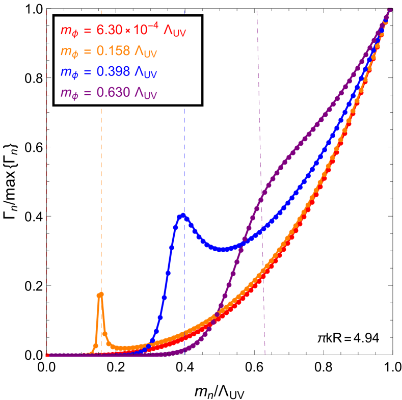
Figure 1: The decay-width spectra obtained for several different choices of our model parameters. The dots of each color indicate the decay widths $\Gamma_{n}$ of the ensemble constituents, normalized to the maximum width $\Gamma_{\rm max}$ obtained for any ensemble constituent with a mass in the range $\hat{m}_{n}\leq\Lambda_{\rm UV}$. The continuous solid curve which connects each set of dots is included simply to guide the eye. The four decay-width spectra shown in the top panel illustrate the effect of varying the AdS curvature scale in the regime in which $m_{\phi}$ is large with $\Lambda_{\rm UV}R=3$ and $m_{\phi}/\Lambda_{\rm UV}=0.398$ held fixed. We observe that as $\pi kR$ increases, a non-monotonicity emerges in the spectrum wherein a local maximum in $\Gamma_{n}$ occurs around $\hat{m}_{n}\sim m_{\phi}$. The four decay-width spectra shown in the bottom panel illustrate the effect of varying $m_{\phi}$ with $\pi kR=4.94$ and $\Lambda_{\rm UV}R=3$ held fixed.

In Fig. 1, in order to show how and where such non-monotonicities can arise within the parameter space of our scenario, we display the decay-width spectra obtained for several different choices of model parameters. The dots of each color indicate the actual $\Gamma_{n}$ values of the $\hat{\chi}_{n}$, and the continuous solid curve connecting these dots is included simply to guide the eye. In order to facilitate comparison between the different spectra, we normalize the decay width of each state in a given ensemble to the maximum decay width

$$\Gamma_{\rm max}~{}\equiv~{}\max_{\hat{m}_{n}\leq\Lambda_{\rm UV}}\{\Gamma_{n}\}$$ (66)

obtained for any ensemble constituent with a mass in the range $\hat{m}_{n}\leq\Lambda_{\rm UV}$. The four decay-width spectra shown in the top panel illustrate the effect of varying the AdS₅ curvature scale in the regime in which $m_{\phi}$ is large. For all spectra shown in the panel, we have fixed $m_{\phi}/\Lambda_{\rm UV}=0.398$ (indicated by the black dashed vertical line) and $\Lambda_{\rm UV}R=3$. The four decay-width spectra shown in the bottom panel illustrate the effect of varying $m_{\phi}$ with $\pi kR=4.94$ and $\Lambda_{\rm UV}R=3$ held fixed. For each of these four spectra, the dashed vertical line of the same color indicates the corresponding value of $m_{\phi}/\Lambda_{\rm UV}$.

We observe from the top panel of Fig. 1 that for small values of $\pi kR$, the decay-width spectrum of the ensemble rises monotonically with $\hat{m}_{n}$, just as it does in the flat-space limit. However, as $\pi kR$ increases, a local maximum in $\Gamma_{n}$ develops around $\hat{m}_{n}\sim m_{\phi}$. This non-monotonicity, which is a consequence of the warping of the extra dimension, is an example of a qualitative feature which does not arise in flat-space DDM scenarios. This behavior is a consequence of the manner in which the projection coefficient $A^{\prime}_{n}$, which is proportional to the value $\hat{\zeta}_{n}(0)=\mathcal{\hat{N}}_{n}[J_{2}(\hat{m}_{n}/k)+\hat{b}_{n}Y_{2}(\hat{m}_{n}/k)]$ of the bulk profile of the corresponding field on the UV brane, varies across the ensemble. Since $|J_{2}(\hat{m}_{n}/k)|\ll|Y_{2}(\hat{m}_{n}/k)|$ in the regime in which $\hat{m}_{n}\ll k$, the magnitude of $A_{n}^{\prime}$ will be maximized in this regime when the constant $\hat{b}_{n}$ is large. While it is not immediately obvious from the form of the expression in Eq. (35) that the value of $\hat{b}_{n}$ is enhanced for ensemble constituents with masses $\hat{m}_{n}\sim m_{\phi}$, we note that this expression can also be recast in the alternative form

$$\hat{b}_{n}~{}=~{}-\left[\frac{m_{B}J_{2}\left(\frac{\hat{m}_{n}}{k}\right)-\hat{m}_{n}J_{1}\left(\frac{\hat{m}_{n}}{k}\right)}{m_{B}Y_{2}\left(\frac{\hat{m}_{n}}{k}\right)-\hat{m}_{n}Y_{1}\left(\frac{\hat{m}_{n}}{k}\right)}\right]~{},$$ (67)

which is obtained applying the boundary condition at $y=0$ in Eq. (40) to $\chi(x,y)$ instead of the boundary condition at $y=\pi R$ in Eq. (31). For $\hat{m}_{n}\ll k$, we may approximate $J_{\alpha}(x)$ and $Y_{\alpha}(x)$ using the standard asymptotic expansions for $x\ll 1$. After some algebra, we find that

$$\hat{b}_{n}~{}\approx~{}\frac{\pi\hat{m}_{n}^{4}}{32k^{4}}\left[\frac{m_{\phi}^{2}(1-e^{-2\pi kR})-8k^{2}}{m_{\phi}^{2}(1-e^{-2\pi kR})-\hat{m}_{n}^{2}}\right]~{}.$$ (68)

We see that within the regime in which $\pi kR$ is large, the denominator in this expression is quite small for $\hat{m}_{n}\sim m_{\phi}$. Indeed, the expression for $\hat{b}_{n}$ in Eq. (68) exhibits a singularity at $\hat{m}_{n}=m_{\phi}(1-e^{-2\pi kR})^{1/2}$, though none of the physical masses for the ensemble constituents ever takes precisely this singular value. As a result, $\hat{b}_{n}$ — and therefore also $A_{n}^{\prime}$ — is sharply peaked for $\hat{\chi}_{n}$ with masses near $m_{\phi}$ in this regime. By contrast, within the regime in which $\pi kR$ is small or vanishing, the asymptotic expansions which led from Eq. (67) to Eq. (68) are not valid. In Appendix A, we derive a general expression for $A_{n}^{\prime}$ in the $\hat{m}_{n}\gg k$ regime using the asymptotic expansions for $J_{\alpha}(x)$ and $Y_{\alpha}(x)$ valid for $x\gg 1$ and show that this expression contains no such singularities.

As $m_{\phi}$ is further increased, the peak in $\Gamma_{n}$ around $\hat{m}_{n}\sim m_{\phi}$ becomes higher and broader. However, for sufficiently large $m_{\phi}$, the decrease in $A^{\prime}_{n}$ with $\hat{m}_{n}$ beyond this peak is more than compensated for by the $\hat{m}_{n}^{2}$ factor in Eq. (62). As a result, the decay-width spectrum once again becomes monotonic in $\hat{m}_{n}$. Thus, we see that both in the regime in which $m_{\phi}\ll m_{\rm KK}$ and in the regime in which $m_{\phi}\sim\Lambda_{\rm UV}$, the scaling relation $\Omega(\Gamma)$ in Eq. (64) can still be meaningfully defined, even for large $\pi kR$. Rather, it is for intermediate values of $m_{\phi}$ that this description breaks down when the warping of the space becomes significant. We note that while $\Gamma_{n}$ scales non-monotonically with $\hat{m}_{n}$, the abundances $\Omega_{n}$ nevertheless scale monotonically. Interestingly, this is the converse of the situation in Ref. DDMThermal , where it is the abundances which scale non-monotonically with mass while the decay widths are monotonic.

Since the parameter $x$ is not well defined across the entire parameter space of our warped-space DDM scenario, we must establish a different method for constraining deviations of the effective equation-of-state parameter $w_{\mathrm{eff}}$ of the ensemble from the constant value $w=0$ which characterizes a stable CDM candidate during the recent cosmological past. In particular, at all times $t_{0}\leq t\leq t_{\mathrm{now}}$, we shall impose the bound condition

$$w_{\mathrm{eff}}(t)~{}<~{}0.05~{}.$$ (69)

Once again, the value $0.05$ has been chosen in accord with the value adopted in Ref. DDMHagedorn in order to ensure that the equation of state for the ensemble does not deviate significantly from that of a stable CDM candidate.

IV.3 Case Study: Small Brane Mass, Strong Warping

Before embarking on a general exploration of the parameter space of our 5D scenario, we begin by focusing on a particular region of interest within that parameter space. In particular, we consider the region in which the AdS curvature scale is large, in the sense that $\pi kR\gg 1$, while $m_{\phi}$ is small in comparison with all other relevant scales in the theory — a criterion which, in the highly-warped regime, is tantamount to requiring that $m_{\phi}\ll m_{\rm KK}$. This region is interesting for several reasons. On the one hand, the region in which $\pi kR\gg 1$ represents the greatest degree of departure from the flat-space limit investigated as a context for DDM model-building in Refs. DDM1 ; DDM2 ; DDMAxion . Moreover, this highly-warped regime corresponds to the regime in the 4D dual theory within which $\Lambda_{\rm UV}/\Lambda_{\rm IR}=e^{\pi kR}$ is large and a significant hierarchy exists between the UV and IR scales. On the other hand as discussed above, the scaling relation $\Omega(\Gamma)$ is nevertheless sensibly defined within the regime in which $m_{\phi}\ll m_{\rm KK}$. Thus, within this region we may compare our results to those obtained in these previous studies in a straightforward manner. Indeed, as we shall demonstrate, the scaling exponents $\alpha(\Gamma)$ and $\beta(\Gamma)$ in Eq. (64) are roughly constant across the range of $\Gamma$ values associated with the lighter constituents in the ensemble which carry the majority of the abundance. Thus, within this region, we can meaningfully define a single value of $x$ with the ensemble.

Within this parameter-space region of interest, the low-lying states within the ensemble include a single extremely light state $\hat{\chi}_{0}$ with a mass $\hat{m}_{0}\sim m_{\phi}$, as well as a large number of additional $\hat{\chi}_{n}$ with masses $k\gg\hat{m}_{n}\gtrsim m_{\rm KK}$. While of course heavier states with $\hat{m}_{n}\geq k$ are also present within the ensemble, the collective abundance of these states is typically so small that the phenomenology of the ensemble is not terribly sensitive to how $\Omega_{n}$ and $\Gamma_{n}$ scale with $\hat{m}_{n}$ across this set of states. Thus, we shall focus on the lighter $\hat{\chi}_{n}$ in deriving a value of $x$ for the ensemble. The expressions for $A_{n}$ and $A^{\prime}_{n}$ for the light states with $n>0$ are given by Eqs. (46) and (48), respectively. Each of these expressions scales with $\hat{m}_{n}$ according to a simple power law. Thus, we find that the abundances of the $\hat{\chi}_{n}$ in our 5D dual theory scale with $\hat{m}_{n}$ according to the relation

$$\Omega_{n}~{}\propto~{}\begin{cases}\hat{m}_{n}^{-1}&\text{instantaneous}\\ \hat{m}_{n}^{-5/2}&\text{staggered (RD era)}\\ \hat{m}_{n}^{-3}&\text{staggered (MD era)}~{},\end{cases}$$ (70)

while the decay widths of these states scale with $\hat{m}_{n}$ according to the relation

$$\Gamma_{n}~{}\propto~{}\hat{m}_{n}^{4}~{}.$$ (71)

Given the results in Eq. (70) and (71), we find that the functional form for $\Omega(\Gamma)$ in this case is

$$\Omega(\Gamma)~{}\propto~{}\begin{cases}\Gamma^{-1/4}&\text{instantaneous}\\ \Gamma^{-5/8}&\text{staggered (RD era)}\\ \Gamma^{-3/4}&\text{staggered (MD era)}~{}.\end{cases}$$ (72)

We emphasize that the scaling relation in Eq. (72) was derived from asymptotic expressions for $A_{n}$ and $A_{n}^{\prime}$ valid only for $n>0$. Within the region of parameter space in which $m_{\phi}$ is much smaller than all other relevant scales in the theory, the abundance $\Omega_{0}$ and decay width $\Gamma_{0}$ of $\hat{\chi}_{0}$ do not accord with this scaling relation. Moreover, within this region of parameter space, $\Omega_{0}$ typically dominates the abundance of the ensemble, while $\Gamma_{0}$ is typically significantly smaller than the decay widths of all of the remaining $\Gamma_{n}$. Indeed, this behavior arises not only in the case of a warped extra dimension, but in the corresponding $mR\ll 1$ regime in the case of a flat extra dimension as well DDM1 . Nevertheless, since $\Omega_{0}$ represents a significant fraction of $\Omega_{\mathrm{tot}}$ within this region, $\hat{\chi}_{0}$ is typically required to be sufficiently long-lived that its decays at $t<t_{\mathrm{now}}$ have a negligible effect on the phenomenology of the ensemble. Rather, it is primarily the $\hat{\chi}_{n}$ with $n>0$ which dictate that phenomenology. Thus, in what follows, we shall focus on the $\hat{\chi}_{n}$ with $n>0$ in deriving an effective value of $x$ for our warped-space DDM ensembles — as was done in the analysis in Ref. DDM1 .

In order to determine the scaling relation for $n_{\Gamma}(\Gamma)$, we begin by noting that the splitting $\hat{m}_{n+1}-\hat{m}_{n}$ between the masses of any two adjacent states $\hat{\chi}_{n+1}$ and $\hat{\chi}_{n}$ is approximately uniform across the ensemble for $n>0$. We are once again primarily interested in the regime in which the mass spectrum is sufficiently dense that we may approximate the density of states per unit mass $n_{m}(m)$ within the ensemble as a function of the continuous variable $m$. Within this regime, a uniform mass splitting implies that $n_{m}(m)$ is approximately constant across the ensemble. The corresponding density of states per unit $\Gamma$ is therefore

$$n_{\Gamma}(\Gamma)~{}=~{}n_{m}(\Gamma)\left(\frac{d\Gamma}{dm}\right)^{-1}~{}\sim~{}\Gamma^{-3/4}~{}.$$ (73)

Combining the results in Eqs. (72) and (73), we find that within the parameter-space region in which $\pi kR\gg 1$ and $m_{\phi}\ll m_{\rm KK}$, the value of $x$ obtained for our ensemble of $\hat{\chi}_{n}$ is

$$x~{}\approx~{}\begin{cases}-1&\text{instantaneous}\\ -11/8&\text{staggered (RD era)}\\ -3/2&\text{staggered (MD era)}~{}.\\ \end{cases}$$ (74)

These results indicate that within this region of parameter space, our ensemble satisfies the the rough consistency criterion $x\lesssim-1$ independent of the details of when the the individual constituents begin oscillating. Thus, we find that ensembles of this sort indeed exhibit an appropriate balancing of decay widths against abundances for DDM. The values of $x$ appearing in Eq. (74), along with the corresponding values of $\alpha$ and $\beta$ obtained in each case, are collected in Table 1 for ease of reference.

IV.4 Generalizing the Scenario

It is possible to generalize the results of the previous section in several ways, even if we wish to restrict our focus to the region of parameter space within which $m_{\phi}$ is much smaller than all other relevant scales in the problem and $x$ is well defined.

Model		Instantaneous			Staggered (RD Era)			Staggered (MD Era)
Brane Mass	SM Fields	$\alpha$	$\beta$	$x$	$\alpha$	$\beta$	$x$	$\alpha$	$\beta$	$x$
UV	UV	$-1/4$	$-3/4$	$-1$	$-5/8$	$-3/4$	$-11/8$	$-3/4$	$-3/4$	$-3/2$
UV	IR	$-1/3$	$-2/3$	$-1$	$-5/6$	$-2/3$	$-3/2$	$-1$	$-2/3$	$-5/3$
IR	UV	$-1/2$	$-3/4$	$-5/4$	$-7/8$	$-3/4$	$-13/8$	$-1$	$-3/4$	$-7/4$
IR	IR	$-2/3$	$-2/3$	$-4/3$	$-7/6$	$-2/3$	$-11/6$	$-4/3$	$-2/3$	$-2$

Table 1: The scaling exponents $\alpha$ and $\beta$ and the parameter $x=\alpha+\beta$ obtained for the four different possible combinations of locations for the brane mass and the SM fields in our 5D scenario within the regime in which $\pi kR\gg 1$ and $m_{\phi}\ll m_{\rm KK}$. Within this regime, $x$ is well defined and approximately constant across a large number of the lower-lying $\hat{\chi}_{n}$ with $n>0$ within the ensemble. Results are shown for three different possible scenarios depending on whether all of the ensemble constituents begin oscillating (and thus behaving as matter rather than as vacuum energy) instantaneously at the time of the mass-generating phase transition, or whether different constituents begin oscillating at different times in staggered fashion after the phase transition has occurred, during either a RD or MD epoch.

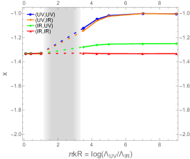
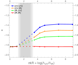
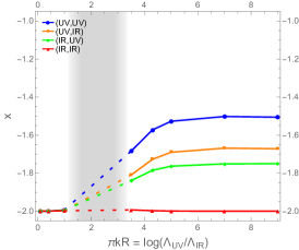
Figure 2: The scaling exponent $x=\alpha+\beta$, plotted as a function of the ratio $\pi kR=\log(\Lambda_{\rm UV}/\Lambda_{\rm IR})$, for the four different possible combinations of locations for the brane mass and the SM fields. All curves shown in all panels of the figure correspond to the same value for the dimensionless product $m_{\phi}R\approx 3.5\times 10^{-4}$. The left, middle, and right panels of the figure correspond respectively to the case in which the $\hat{\chi}_{n}$ all begin oscillating instantaneously at the time of the mass-generating phase transition, the case in which the $t_{n}$ are staggered in time during a RD epoch, and the case in which the $t_{n}$ are staggered in time during a MD epoch. We observe that all of the curves shown in each panel approach a common $x$ value in the flat-space limit, which corresponds to taking $\pi kR\rightarrow 0$.

Thus far, we have focused on the case in which the fields of the SM and the dynamics which generates $m_{\phi}$ are both localized on the UV brane. However, we are also free to consider alternative possibilities in which this dynamics, the SM fields, or both are instead localized on the IR brane. Such modifications of our scenario can have a significant impact on $\Omega(\Gamma)$ and $n_{\Gamma}(\Gamma)$. For example, if the SM fields are localized on the IR brane, it is not the projection coefficients $A^{\prime}_{n}$ which determine the decay widths of our ensemble constituents, but rather a different set of coefficients $A_{n}^{\prime\prime}\equiv e^{-4\pi kR}\sqrt{1-e^{-2\pi kR}}/\sqrt{2k}\langle\chi(x,\pi R)|\hat{\chi}_{n}\rangle$ which represent the projection of the $\hat{\chi}_{n}$ onto the IR brane at $y=\pi R$. A detailed derivation of the values of $\alpha$ and $\beta$ for each of the four possible combinations of locations for the brane mass and the SM fields is provided in Appendix B. Once again, in deriving these scaling exponents, we focus on the regime in which $\pi kR\gg 1$ and $m_{\phi}\ll m_{\rm KK}$. The main results are summarized in Table 1.

It is also interesting to consider how the results in Table 1 are modified when we depart from the $\pi kR\gg 1$ regime. However, while the parameter $x$ is always well defined within the region of parameter space wherein $m_{\phi}$ is much smaller than all other relevant scales in the problem, regardless of the value of $\pi kR$, it is not always constant. Thus, in assessing how our results for $x$ generalize for arbitrary values of $\pi kR$, we must first identify the regions of parameter space within which $x$ is constant across a large number of the lower-lying $\hat{\chi}_{n}$ with $n>0$ within the ensemble, since it is only within these regions where we can meaningfully associate a single value of $x$ with the ensemble. We have already seen that this is the case within the regime wherein $\pi kR\gg 1$. For $\pi kR$ outside this regime, however, the number of states with masses $k\gg\hat{m}_{n}\gtrsim m_{\rm KK}$ is far smaller. When this is the case, $x$ is not necessarily constant even across the lightest several $\hat{\chi}_{n}$ with $n>0$ in the ensemble. That said, we also note that for $\pi kR\lesssim 1$, all of the low-lying $\hat{\chi}_{n}$ with $n>0$ have $\hat{m}_{n}\gtrsim k$. As a result, $x$ is approximately constant across this portion of the ensemble within this regime. Thus, it is once again sensible from a DDM perspective to identify this value of $x$ as the effective value of $x$ for the ensemble.

Given these considerations, we adopt the following procedure in analyzing how $x$ varies as a function of $\pi kR$. We calculate a value of $x$ only for those ensembles for which the masses of the $\hat{\chi}_{n}$ with $1\leq n\leq 10$ either all satisfy the condition $\hat{m}_{n}\leq k$ or else all satisfy the condition $\hat{m}_{n}\geq k$. We then calculate $x$ by performing linear fits of both $\log(A_{n})$ and $\log(A_{n}^{\prime})$ to $\log(\hat{m}_{n})$ for the set of ensemble constituents $\hat{\chi}_{n}$ with $2\leq n\leq 9$. In this way, we may define an effective value of $x$ for all $\pi kR$ either above or below the rough range $1\lesssim\pi kR\lesssim 3$.

In Fig. 2, we plot this effective value of $x$ as a function of $\pi kR=\log(\Lambda_{\rm UV}/\Lambda_{\rm IR})$ for all four possible combinations of locations for the brane mass and the SM fields. The results shown in the left, middle, and right panels of the figure correspond respectively to the case in which the $\hat{\chi}_{n}$ all begin oscillating instantaneously at $t_{n}=t_{G}$, the case in which the $t_{n}$ are staggered in time during a RD epoch, and the case in which the $t_{n}$ are staggered in time during a MD epoch. All points displayed in all panels of the figure correspond to the same value for the dimensionless product $m_{\phi}R\approx 3.5\times 10^{-4}$ — a value chosen such that $m_{\phi}=m_{\rm KK}$ for the largest value of $\pi kR$ within the range $0\leq\pi kR\leq 9$ included in each plot. This parameter choice ensures that $m_{\phi}\ll\hat{m}_{n}$ for all $n>1$ across this entire range of $\pi kR$. While we have connected these points in order to guide the eye, we emphasize that we have only included $x$ values for $\pi kR$ within the ranges $\pi kR\lesssim 1$ and $\pi kR\gtrsim 3$ wherein this quantity is sensibly defined.

For all of the curves shown in Fig. 2, we observe that the value of $x$ rapidly approaches the corresponding asymptotic value quoted in Table 1 as $\pi kR\gtrsim 1$. Moreover, we see that the values of $x$ obtained for $\pi kR=9$ accord well with this asymptotic value in all cases. By contrast, we see in each panel that as $\pi kR\rightarrow 0$, the values of $x$ obtained for all possible combinations of brane-mass and SM-field locations asymptote to a single, common value. This common value is precisely the value of $x$ obtained in Ref. DDM1 for the corresponding oscillation-onset behavior in the flat-space limit: $x=-4/3$ for an instantaneous turn-on, $x=-11/10$ and for a staggered turn-on during a RD epoch, and $x=-2$ for a staggered turn-on during a MD epoch.

IV.5 Surveying the Parameter Space

We now turn to examine how the bounds in Eqs. (63) and (69) constrain the full parameter space of our ensemble. We shall assume that the lightest ensemble constituent begins oscillating well before the beginning of the BBN epoch — i.e., that $t_{0}\ll t_{\rm BBN}$. When evaluating $\Omega_{\mathrm{tot}}$ and $w_{\mathrm{eff}}$ during the RD era prior to $t_{\mathrm{MRE}}$, we take our fiducial time $t_{\ast}$ in Eqs. (57) and (61) to be some early time $t_{0}\leq t_{\ast}\ll t_{\rm BBN}$. Thus, for all $t_{\rm BBN}\leq t\leq t_{\mathrm{MRE}}$, we may approximate $t-t_{\ast}\approx t$. For simplicity, at all times $t>t_{\mathrm{MRE}}$, we ignore the effect of dark energy on $H$ at late times $t\sim t_{\mathrm{now}}$ and approximate the universe as strictly MD. We also ignore any back-reaction on $H$ which results from the decay of the ensemble itself during this MD era, even though $\rho_{\mathrm{tot}}$ dominates the energy density of the universe at this time, given that we shall be imposing the bound in Eq. (63) and thereby mandating that $\rho_{\mathrm{tot}}$ does not differ significantly from the prediction of the $\Lambda$CDM cosmology. With these approximations, $\Omega_{\mathrm{tot}}$ and $w_{\mathrm{eff}}$ are given by Eqs. (57) and (61) at times $t<t_{\mathrm{MRE}}$, but with $\kappa=2$ rather than $\kappa=3/2$. When evaluating $\Omega_{\mathrm{tot}}$ and $w_{\mathrm{eff}}$ during this MD era, we take $t_{\ast}=t_{\mathrm{MRE}}$. However, since $\Omega_{n}(t_{\mathrm{MRE}})\propto\Omega_{n}^{0}e^{-\Gamma_{n}(t-t_{0})}$, where the constant of proportionality is the same for all $\hat{\chi}_{n}$ and is independent of the background cosmology, we find that the ratio $\Omega_{\mathrm{tot}}/\widetilde{\Omega}_{\rm tot}$ at any time $t_{\rm BBN}<t\leq t_{\mathrm{now}}$, regardless of the relationship between $t$ and $t_{\mathrm{MRE}}$, is given by

$$\frac{\Omega_{\mathrm{tot}}}{\widetilde{\Omega}_{\rm tot}}~{}\approx~{}\frac{\sum_{n=0}^{\infty}\Omega_{n}^{0}e^{-\Gamma_{n}t}}{\sum_{n=0}^{\infty}\Omega_{n}^{0}}~{}.$$ (75)

By contrast, the effective equation-of-state parameter for the ensemble is given by

$$w_{\mathrm{eff}}~{}\approx~{}\frac{\sum_{n=0}^{\infty}\Omega_{n}^{0}\Gamma_{n}te^{-\Gamma_{n}t}}{\sum_{n=0}^{\infty}\Omega_{n}^{0}e^{-\Gamma_{n}t}}\times\begin{cases}2/3&t<t_{\mathrm{MRE}}\\ 1/2&t>t_{\mathrm{MRE}}~{}.\end{cases}$$ (76)

We note that while our expressions for $w_{\mathrm{eff}}$ before and after matter-radiation equality are not equal at $t=t_{\mathrm{MRE}}$, this apparent discontinuity in $w_{\mathrm{eff}}$ is simply a reflection of the fact that we are approximating the transition from the RD era to the MD era as an instantaneous event occurring at time $t=t_{\mathrm{MRE}}$, at which point the Hubble parameter leaps discontinuously from $H=1/(2t)$ to $H=2/(3t)$. In reality, of course, $H$ transitions continuously between these asymptotic values at $t\sim t_{\mathrm{MRE}}$. In order to describe the evolution of $w_{\mathrm{eff}}$ during this transition, one would need to treat the parameter $\kappa$ as a function of $t$. However, since we are only interested in bounding $w_{\mathrm{eff}}$ and not its time derivatives, approximating this transition as instantaneous is sufficient for our purposes.

In assessing how the constraints in Eqs. (63) and (69) impact the parameter space of our scenario, we begin by noting that the expression for $\Omega_{\mathrm{tot}}/\widetilde{\Omega}_{\rm tot}$ in Eq. (75) depends on the physical scales $\Gamma_{0}$ and $t$ only through the dimensionless quantity $\sigma\equiv\Gamma_{0}t$. Indeed, we observe that

$$\frac{\Omega_{\mathrm{tot}}}{\widetilde{\Omega}_{\rm tot}}~{}\approx~{}\frac{\sum_{n=0}^{\infty}\Omega_{n}^{0}e^{-\frac{\Gamma_{n}}{\Gamma_{0}}\sigma}}{\sum_{n=0}^{\infty}\Omega_{n}^{0}}~{},$$ (77)

which depends on $\sigma$ and on the ratios $\Gamma_{n}/\Gamma_{0}=\hat{m}_{n}^{3}A_{n}^{\prime 2}/(\hat{m}_{0}^{3}A_{0}^{\prime 2})$ of the decay widths of the ensemble constituents, but not on the value of $\Gamma_{0}$ itself. Likewise, our expression for $w_{\mathrm{eff}}$ in Eq. (76) can be written as

$$w_{\mathrm{eff}}~{}\approx~{}\frac{\sum_{n=0}^{\infty}\Omega_{n}^{0}\frac{\Gamma_{n}}{\Gamma_{0}}\sigma e^{-\frac{\Gamma_{n}}{\Gamma_{0}}\sigma}}{\sum_{n=0}^{\infty}\Omega_{n}^{0}e^{-\frac{\Gamma_{n}}{\Gamma_{0}}\sigma}}\times\begin{cases}2/3&\sigma<\Gamma_{0}t_{\mathrm{MRE}}\\ 1/2&\sigma>\Gamma_{0}t_{\mathrm{MRE}}~{},\end{cases}$$ (78)

which depends on the value of $\Gamma_{0}$ only in that this parameter determines the value of $\sigma$ at the time of matter-radiation equality. Moreover, we note that the expression for $w_{\mathrm{eff}}$ at times $t<t_{\mathrm{MRE}}$ is always larger than the corresponding expression at times $t>t_{\mathrm{MRE}}$ by an overall multiplicative factor of precisely $4/3$. Given this, we shall hereafter adopt a conservative approach in establishing bounds on $w_{\mathrm{eff}}$ in which we always treat $w_{\mathrm{eff}}$ as being given by the expression valid during the RD era prior to matter-radiation equality, regardless of the actual relationship between $t$ and $t_{\mathrm{MRE}}$. With this modification, our expressions for both $\Omega_{\mathrm{tot}}$ and $w_{\mathrm{eff}}$ depend only on $\sigma$, and not on $\Gamma_{0}$ and $t$ independently. In other words, these expressions are invariant under any simultaneous rescaling of $\Gamma_{0}$ and $t$ which leaves their product invariant.

The utility of this invariance is perhaps best conveyed in the context of a graphical example. In Fig. 3, we show how $w_{\mathrm{eff}}(\sigma)$ and $\Omega_{\mathrm{tot}}(\sigma)$ actually evolve as functions of $\sigma$ for four different choices of $m_{\phi}R$ and $\pi kR$. These four choices are intended to exemplify different possible regimes for these two parameters. In particular, these choices are representative of the regimes in which $\pi kR$ and $m_{\phi}R$ are both small (first row), in which $\pi kR$ is small but $\pi kR$ is large (second row), in which $\pi kR$ is large but $m_{\phi}R$ is small (third row), and in which $\pi kR$ and $m_{\phi}R$ are both large (fourth row). In all cases, we have taken $\Lambda_{\rm UV}R=3$ and assumed that all of the $\hat{\chi}_{n}$ begin oscillating instantaneously at $t=t_{0}$. In each panel, the blue line indicates the value of the quantity $w_{\mathrm{eff}}(\sigma)$ or $\Omega_{\mathrm{tot}}(\sigma)$ itself, while the black dashed line indicates the corresponding constraint from either Eq. (69) or Eq. (63). The vertical red lines indicate the values $\sigma_{n}\equiv\Gamma_{0}\tau_{n}$ of the dimensionless time variable $\sigma$ which correspond to the lifetimes of the $\hat{\chi}_{n}$ with $\hat{m}_{n}\leq\Lambda_{\rm UV}$.

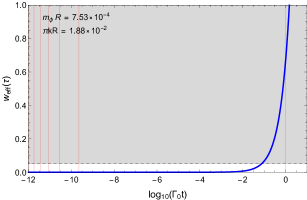
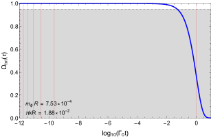
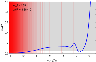
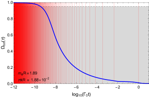
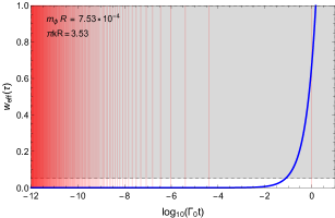
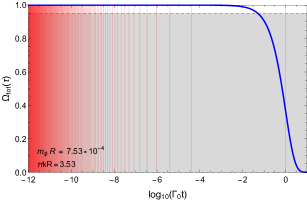
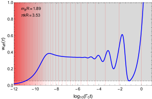
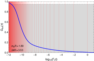
Figure 3: The effective ensemble equation-of-state parameter $w_{\mathrm{eff}}(\sigma)$ (left panel in each row) and total ensemble abundance $\Omega_{\mathrm{tot}}(\sigma)$ (right panel in each row), plotted as functions of $\sigma\equiv\Gamma_{0}t$. Each row of the figure corresponds to a particular choice of $\pi kR$ and $m_{\phi}R$. These choices are representative of the regimes in which $\pi kR$ and $m_{\phi}R$ are both small (first row), in which $\pi kR$ is small but $\pi kR$ is large (second row), in which $\pi kR$ is large but $m_{\phi}R$ is small (third row), and in which $\pi kR$ and $m_{\phi}R$ are both large (fourth row). In all cases, we have taken $\Lambda_{\rm UV}R=3$ and assumed that all of the $\hat{\chi}_{n}$ begin oscillating instantaneously at $t=t_{0}$. In each panel, the blue line is the value of the quantity $w_{\mathrm{eff}}$ or $\Omega_{\mathrm{tot}}$ itself, while the black dashed line indicates the corresponding constraint from either Eq. (69) or (63). The red vertical lines indicate the values $\sigma_{n}=\Gamma_{0}\tau_{n}$ of $\sigma$ at which the various $\hat{\chi}_{n}$ decay. The gray regions are excluded by the constraints. In particular, for any given ensemble, consistency with these constraints requires that $\Gamma_{0}$ be taken sufficiently small that for all $\sigma$ within the range $\sigma<\sigma_{\rm now}\equiv\Gamma_{0}t_{\mathrm{now}}$, the blue curves for both $w_{\mathrm{eff}}$ and $\Omega_{\mathrm{tot}}$ do not enter the gray region.

In interpreting the results shown in Fig. 3, we begin by observing that while reciprocal rescalings of $\Gamma_{0}$ and $t$ do not affect the overall shapes of the curves representing $w_{\mathrm{eff}}$ and $\Omega_{\mathrm{tot}}/\widetilde{\Omega}_{\rm tot}$ as functions of $\sigma$, such rescalings do change the value $\sigma_{\rm now}\equiv\Gamma_{0}t_{\mathrm{now}}$ of $\sigma$ which corresponds to present time. In particular, the smaller $\Gamma_{0}$ is, the smaller the corresponding value of $\sigma_{\rm now}$. Consistency with the constraints in Eqs. (63) and (69) requires only that these constraints be satisfied for $\sigma<\sigma_{\rm now}$. The results shown in each row of Fig. 3 therefore suggest that these constraints can generally be satisfied by choosing a sufficiently small value for $\Gamma_{0}$ that the blue curves for both $w_{\mathrm{eff}}$ and $\Omega_{\mathrm{tot}}$ never enter the respective gray regions for all $\sigma$ within the range $\sigma<\sigma_{\rm now}$. Indeed, we observe that consistency with these constraints can always be achieved by taking $\Gamma_{0}$ to be sufficiently small, provided either that the number of $\hat{\chi}_{n}$ in the ensemble is finite and that their lifetimes satisfy $t_{0}\ll\tau_{0}$, or else that the $\hat{\chi}_{n}$ with lifetimes $\tau_{n}\lesssim t_{0}$ collectively contribute only a negligible fraction of the total abundance of the ensemble at $t=t_{0}$.

Thus, when this is the case, we see that the constraints in Eqs. (69) and (63) do not simply serve to exclude particular combinations of the model parameters $\pi kR$, $m_{\phi}$, and $\Lambda_{\rm UV}R$ outright, but rather to establish an upper bound on $\Gamma_{0}$ — or, equivalently, a lower bound on $\tau_{0}$ — for any such combination of these parameters. More explicitly, the maximum value $\sigma_{\rm now}^{\rm max}$ of $\sigma_{\rm now}$ for which these constraints are simultaneously satisfied determines the minimum possible lifetime $\tau_{0}^{\rm min}$ for the lightest ensemble constituent through the relation

$$\tau_{0}^{\rm min}~{}=~{}\frac{t_{\mathrm{now}}}{\sigma_{\rm now}^{\rm max}}~{}.$$ (79)

We stress that $\tau_{0}$ is indeed an independent degree of freedom in this scenario. Although the overall normalization factors for both the abundances and lifetimes of the $\hat{\chi}_{n}$ both depend on $\hat{f}_{X}$, the normalization factor for the $\Omega_{n}$ depends not only on additional model parameters, such as the misalignment angle $\theta$, but also on the details of the cosmological history at times $t>t_{0}$.

It is also worth remarking that the results shown in the top two rows of Fig. 3 are qualitatively similar to those obtained in the $k\rightarrow 0$ limit studied in Ref. DDM1 . The last two rows of the figure correspond to cases in which $\pi kR$ is large and therefore represent departures from the flat-space case. We observe that it is when $\pi kR$ and $m_{\phi}R$ are both large that the deviations from the CDM limit are the most dramatic.

We now survey the parameter space of our model, using the criterion in Eq. (79) in order to establish a bound on $\tau_{0}$ at each point within that parameter space. In particular, we hold $\Lambda_{\rm UV}R$ fixed and vary both $\pi kR$ and $m_{\phi}R$. In Fig. 5, we show contours in $(\pi kR,m_{\phi}R)$-space of $\tau_{0}^{\rm min}$ for the parameter choice $\Lambda_{\rm UV}R=3$. The different panels of the figure correspond to the three different behaviors for the oscillation-onset times delineated in Eq. (52). In particular, the left, middle, and right panels of the figure respectively correspond to the case of an instantaneous turn-on, a staggered turn-on during a RD era, and a staggered turn-on during an MD era.

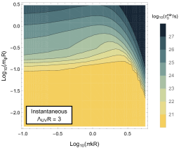
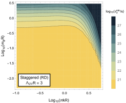
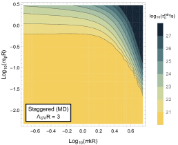
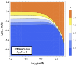
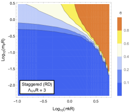
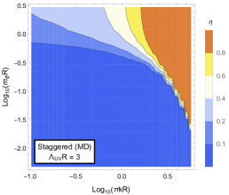
Figure 4: Contours of the minimum lifetime $t_{0}^{\rm min}$ consistent with the constraints in Eqs. (69) and (63), plotted within the $(\pi kR,m_{\phi}R)$-plane. For this plot, we take $\Lambda_{\rm UV}R=3$. The left, middle, and right panels respectively correspond to the case of an instantaneous turn-on, a staggered turn-on during a radiation-dominated era, and a staggered turn-on during a matter-dominated era. We see that in general, the bound on $\tau_{0}$ becomes increasingly stringent as the degree of warping is increased for fixed $m_{\phi}R$.

Figure 5: Contours of the initial value $\eta(t_{0})$ of the DDM tower fraction, plotted within the same $(\pi kR,m_{\phi}R)$-plane shown in Fig. 5. Once again, we take $\Lambda_{\rm UV}R=3$.

Generally speaking, we observe that in each panel of the figure, the bound on $\tau_{0}$ tends to become more stringent as $\pi kR$ is increased for a fixed value of $m_{\phi}R$. This implies that for a given choice of the parameter $\tau_{0}$, there is a maximum degree of AdS warping for which a phenomenologically consistent dark sector can emerge for any fixed value of $m_{\phi}R$. Moreover, we observe that the bound on the AdS curvature scale generally becomes more and more stringent as $m_{\phi}R$ is increased, in agreement with the results shown in Fig. 3. Indeed, the regime in which $\pi kR$ and $m_{\phi}R$ are both large is the regime in which a significant number of low-lying states with similar abundances and comparable lifetimes are present within the ensemble. Moreover, comparing results across the three panels of the figure, we see that the bounds are more stringent for the case of an instantaneous turn-on than they are for the case of a staggered turn-on during either a RD or MD era. Indeed, this is expected, since the $\Omega_{n}^{0}$ for the lighter $\hat{\chi}_{n}$ are enhanced relative to the $\Omega_{n}^{0}$ for the heavier $\hat{\chi}_{n}$ in the case of a staggered turn-on. These lighter modes, which typically have longer lifetimes, therefore carry a larger fraction of $\Omega_{\mathrm{tot}}$ in this case than in the case of an instantaneous turn-on, and as a result the ensemble as a whole is more stable.

While the results in Fig. 5 provide a great deal of information about the ensembles which arise within the parameter space of our warped-space scenario, there are other considerations which we must also take into account in assessing which regions of that parameter space are phenomenologically of interest. In particular, from a DDM perspective, we are interested in ensembles which are not only consistent with observational constraints, but which also represent a significant departure from traditional dark-matter scenarios — scenarios in which a single particle species contributes essentially the entirety of the dark-matter abundance. The degree to which the contribution from the most abundant individual constituent dominates in $\Omega_{\mathrm{tot}}$ at any given time can be be parametrized by the “tower fraction” $\eta$, defined by the relation DDM1

$$\eta(t)~{}\equiv~{}\frac{\Omega_{\mathrm{tot}}-\max_{n}\{\Omega_{n}\}}{\Omega_{\mathrm{tot}}}~{},$$ (80)

the range of which is $0\leq\eta<1$. If the most abundant individual ensemble constituent contributes essentially the entirety of $\Omega_{\mathrm{tot}}$, with the other $\hat{\chi}_{n}$ contributing negligibly to this total abundance, then $\eta\ll 1$ and this individual ensemble constituent is for all intents and purposes a single-particle dark-matter candidate. By contrast, if $\eta\sim\mathcal{O}(1)$, multiple $\hat{\chi}_{n}$ contribute meaningfully to $\Omega_{\mathrm{tot}}$ and the ensemble is truly DDM-like.

In Fig. 5 we show contours of the initial value $\eta(t_{0})$ of the tower fraction at the time at which the abundances $\Omega_{n}$ are effectively established within the same region of parameter space as in Fig. 5, and for the same choice of $\Lambda_{\rm UV}R$. While the present-day tower fraction $\eta(t_{\mathrm{now}})$ differs from $\eta(t_{0})$ as a result of $\hat{\chi}_{n}$ decays, this difference is generally not terribly significant for ensembles which satisfy the constraint on $\Omega_{\mathrm{tot}}$ in Eq. (63).

One important feature that emerges upon comparing Figs. 5 and 5 is that the conditions which make $\eta(t_{0})$ large are also those which make the bound on $\tau_{0}$ quite stringent. In other words, there is an increasing tension between these two figures as $\pi kR$ gets large. Indeed, if we impose an upper bound on $\tau_{0}$ (so that our DDM ensemble continues to be dynamical throughout up to and including the present epoch) as well as a lower bound on $\eta(t_{0})$ (so that our scenario remains “DDM-like,” with a significant fraction of the total dark-matter abundance shared across many ensemble constituents), then for any value of $m_{\phi}R$ there exists a maximum value of warping which may be tolerated. Fortunately, however, we also observe that it is nevertheless possible to achieve a reasonably large value of $\eta(t_{0})$ without requiring the value of $\tau_{0}$ to be extreme.

We also note that for $\pi kR\ll 1$, the values of $\eta(t_{0})$, expressed as functions of $m_{\phi}R$, are in complete agreement with the flat-space results previously found in Ref. DDM1 . Thus, in this sense, we may view the contour plots in Fig. 5 as illustrating the structure that emerges as we move away from the flat-space limit and increase $\pi kR$.

V Warped vs. Flat from the Dual Perspective

Thus far, we have examined a 5D theory involving a bulk scalar propagating within a slice of AdS₅ and have shown that the mixed KK modes of this bulk scalar are capable of satisfying the basic criteria for a phenomenologically viable DDM ensemble in which multiple constituents contribute meaningfully to $\Omega_{\mathrm{tot}}$. This in turn implies that the ensemble of partially composite scalars which arises in the 4D dual of this warped-space theory can likewise serve as a DDM ensemble as well. Thus, we have demonstrated what we set out to demonstrate in this paper — namely that scenarios involving such ensembles are a viable context for model-bulding within the DDM framework.

There are, however, certain aspects of the AdS/CFT dictionary that relates the two dual theories which deserve further comment. Within the regime in which the AdS curvature scale is large, this dictionary is reasonably transparent. In general, the two dimensionful parameters $k$ and $R$ which characterize the 5D theory at times $t\lesssim t_{G}$ are related to the physical scales $\Lambda_{\rm UV}$ and $\Lambda_{\rm IR}$ of the strongly-coupled 4D theory by

$$\Lambda_{\rm IR}~{}=~{}\Lambda_{\rm UV}\,e^{-\pi kR}~{}.$$ (81)

Thus, as briefly mentioned in Sect. IV, the regime in which $\pi kR\gg 1$ corresponds to a large hierarchy between $\Lambda_{\rm IR}$ and $\Lambda_{\rm UV}$. The lightest mass eigenstate $\hat{\chi}_{0}$ in the 5D theory corresponds to a state in the 4D theory which is primarily elementary. The rest of the low-lying $\hat{\chi}_{n}$ in the 5D theory correspond to states in the 4D theory which are primarily composite.

By contrast, within the regime in which $\pi kR\ll 1$ and the theory approaches the flat-space limit considered in Ref. DDM1 , the relationship between the states of the 4D and 5D theories is more subtle. The corresponding regime in the 4D theory is that in which $\Lambda_{\rm IR}\approx\Lambda_{\rm UV}$. The KK eigenstates $\hat{\chi}_{n}^{(k=0)}$ which emerge in the flat-space limit of our warped DDM scenario do not correspond to composite states of the CFT in the dual 4D theory. Rather, these states correspond to a tower of elementary fields $\phi_{n}$ with masses $M_{n}\sim n/R$ which are also generically present in the theory and mix with the $\varphi_{n}$. Indeed, the elementary scalar $\phi_{0}$ introduced in Sect. II may be viewed as the lightest of these fields. The $\phi_{n}$ with $n>0$ typically do not play a significant role in the phenomenology of the partially composite theory when $\Lambda_{\rm IR}\ll\Lambda_{\rm UV}$. The reason is that within this regime a large number of light states are present in the ensemble with masses $\hat{m}_{n}\ll 1/R$. These light states have negligible wavefunction overlap with any of the $\phi_{n}$ other than $\phi_{0}$. However, in the opposite regime in which $\Lambda_{\rm IR}\approx\Lambda_{\rm UV}$, no such hierarchy exists between the mass scales of the elementary and composite states of the 4D theory. Within this regime, the $\phi_{n}$ do indeed play an important role in the phenomenology of the model.

In order to understand how the $\phi_{n}$ affect the properties of the DDM ensemble in the $\Lambda_{\rm IR}\approx\Lambda_{\rm UV}$ regime, it is illustrative to compare the structure of the mass matrix which emerges in this regime to the structure which emerges in the $\Lambda_{\rm IR}\ll\Lambda_{\rm UV}$ regime. In situations in which the $\varphi_{n}$ are all significantly heavier than at least the lightest several $\phi_{n}$, the mass eigenstates $\chi_{n}$ of the theory at times $t\lesssim t_{G}$ are simply the $\phi_{n}$, with the corresponding masses $m_{0}=0$ for $n=0$ and $m_{n}=M_{n}$ for $n>0$. By contrast, at times $t\gtrsim t_{G}$, the squared-mass matrix in the $\phi_{n}$ basis has the rough overall structure

$$\mathcal{M}^{2}~{}=~{}\left(\begin{matrix}m_{\phi}^{2}&m_{\phi}^{2}&m_{\phi}^{2}&\ldots\\ m_{\phi}^{2}&M_{1}^{2}+m_{\phi}^{2}&m_{\phi}^{2}&\ldots\\ m_{\phi}^{2}&m_{\phi}^{2}&M_{2}^{2}+m_{\phi}^{2}&\ldots\\ \vdots&\vdots&\vdots&\ddots\end{matrix}\right)~{}.$$ (82)

In the regime in which $m_{\phi}\ll M_{n}$ for all $n>0$, the mass eigenstates $\hat{\chi}_{n}$ are, to $\mathcal{O}(m_{\phi}^{2}/M_{n}^{2})$, given by

$$|\hat{\chi}_{n}\rangle~{}\approx~{}\begin{cases}|\phi_{0}\rangle-{\displaystyle\sum_{\ell=1}^{\infty}}\frac{m_{\phi}^{2}}{M_{\ell}^{2}}|\phi_{\ell}\rangle&n=0\\ \frac{m_{\phi}^{2}}{M_{n}^{2}}|\phi_{0}\rangle+|\phi_{n}\rangle+{\displaystyle\sum_{\ell\neq 0,n}^{\infty}}\frac{m_{\phi}^{2}}{M_{n}^{2}-M_{\ell}^{2}}|\phi_{\ell}\rangle&n>0~{}.\end{cases}$$ (83)

To the same order, the corresponding mass eigenvalues are $\hat{m}_{0}^{2}\approx m_{\phi}^{2}$ for $n=0$ and $\hat{m}_{n}^{2}\approx M_{n}^{2}+m_{\phi}^{2}$ for $n>0$.

Since all of the $\chi_{n}$ with $n>0$ are massive prior to the phase transition, only $\chi_{0}$ can acquire a misaligned vacuum value. Thus, the mixing coefficients $A_{n}=\langle\chi_{0}|\hat{\chi}_{n}\rangle$ play the same phenomenological role in the $\Lambda_{\rm IR}\approx\Lambda_{\rm UV}$ regime as they do in the $\Lambda_{\rm IR}\ll\Lambda_{\rm UV}$ regime. In our truncated theory, these coefficients are given by

$$A_{n}~{}=~{}\langle\phi_{0}|\hat{\chi}_{n}\rangle~{}\approx~{}\begin{cases}1&n=0\\ \frac{m_{\phi}^{2}}{M_{n}^{2}}&n>0~{}.\end{cases}$$ (84)

The projection coefficients $A_{n}^{\prime}$ in this same regime are

$$A_{n}^{\prime}~{}=~{}\sum_{\ell=0}^{\infty}\langle\phi_{\ell}|\hat{\chi}_{n}\rangle~{}\approx~{}\langle\phi_{n}|\hat{\chi}_{n}\rangle~{}\approx~{}1~{},$$ (85)

up to corrections of $\mathcal{O}(m_{\phi}^{2}/M_{n}^{2})$. These results agree with those in Ref. DDM1 for the $m_{\phi}\ll M_{n}$ regime, up to $\mathcal{O}(1)$ numerical factors. Of course, for $m_{\phi}$ outside this regime, the full, infinite-dimensional mass matrix is required in order to obtain the corresponding expressions for $A_{n}$ and $A_{n}^{\prime}$.

The structure of the mass-squared matrix in Eq. (82) clearly differs in several ways from the structure of the mass-squared matrix in Eq. (17) for the corresponding truncated theory within the $\Lambda_{\rm IR}\ll\Lambda_{\rm UV}$ regime. However, the mass-squared matrices in Eqs. (82) and (17) cannot meaningfully be compared because the former is expressed with respect to the basis of mass eigenstates prior to the phase transition, whereas the latter is expressed in the $\{\phi_{0},\varphi_{n}\}$ basis. Rather, the mass-squared matrix in Eq. (82) must be compared to the mass-squared matrix $\widetilde{\mathcal{M}}^{2}$ obtained in the $\Lambda_{\rm IR}\ll\Lambda_{\rm UV}$ regime after the phase transition expressed in the basis of the states $\chi_{n}$ which are mass eigenstates of the theory before the phase transition. This matrix is given by $\widetilde{\mathcal{M}}^{2}=\mathcal{U}\mathcal{M}^{2}\mathcal{U}^{\dagger}$, where $\mathcal{M}^{2}$ is the matrix appearing in Eq. (17) and $\mathcal{U}$ is the unitary matrix which represents the transformation from the $\{\phi_{0},\varphi_{n}\}$ basis to the $\chi_{n}$ basis. The results in Eq. (14) imply that to $\mathcal{O}(\epsilon_{n}^{2})$, this latter matrix is given by

$$\mathcal{U}~{}\approx~{}\left(\begin{matrix}1-\sum_{m=1}^{\infty}\frac{\epsilon_{m}^{2}}{2g_{m}^{2}}&-\frac{\epsilon_{1}}{g_{1}}&-\frac{\epsilon_{2}}{g_{2}}&\ldots\\ \frac{\epsilon_{1}}{g_{1}}&1-\frac{\epsilon_{1}^{2}}{2g_{1}^{2}}&\frac{\epsilon_{1}\epsilon_{2}g_{2}}{g_{1}(g_{1}^{2}-g_{2}^{2})}&\ldots\\ \frac{\epsilon_{2}}{g_{2}}&\frac{\epsilon_{2}\epsilon_{1}g_{1}}{g_{2}(g_{2}^{2}-g_{1}^{2})}&1-\frac{\epsilon_{2}^{2}}{2g_{2}^{2}}&\ldots\\ \vdots&\vdots&\vdots&\ddots\end{matrix}\right)~{}.$$ (86)

As a result, to the same order in $\epsilon_{n}$, we find that

$$\widetilde{\mathcal{M}}^{2}~{}\approx~{}\left(\begin{matrix}m_{\phi}^{2}\left(1+\sum_{m=1}^{\infty}\frac{\epsilon_{m}^{2}}{g_{m}^{2}}\right)&\frac{\epsilon_{1}}{g_{1}}m_{\phi}^{2}&\frac{\epsilon_{2}}{g_{2}}m_{\phi}^{2}&\ldots\\ \frac{\epsilon_{1}}{g_{1}}m_{\phi}^{2}&(g_{1}^{2}+\epsilon_{1}^{2})\Lambda_{\rm IR}^{2}+\frac{\epsilon_{1}^{2}}{g_{1}^{2}}m_{\phi}^{2}&\frac{\epsilon_{1}\epsilon_{2}}{g_{1}g_{2}}m_{\phi}^{2}&\ldots\\ \frac{\epsilon_{2}}{g_{2}}m_{\phi}^{2}&\frac{\epsilon_{1}\epsilon_{2}}{g_{1}g_{2}}m_{\phi}^{2}&(g_{2}^{2}+\epsilon_{2}^{2})\Lambda_{\rm IR}^{2}+\frac{\epsilon_{2}^{2}}{g_{2}^{2}}m_{\phi}^{2}&\ldots\\ \vdots&\vdots&\vdots&\ddots\end{matrix}\right)~{}.$$ (87)

Comparing the results in Eqs. (82) and (87), we see that the crucial difference between the structures of these two mass-squared matrices is due to the factors of $\epsilon_{n}/g_{n}$ that appear in both the diagonal and off-diagonal contributions to $\widetilde{\mathcal{M}}^{2}$ which arise a result of the phase transition. These factors arise in the $\Lambda_{\rm IR}\ll\Lambda_{\rm UV}$ regime as a consequence of the coupling between $\phi_{0}$ and the composite sector engendered by the operator $\mathcal{O}_{c}$. The fact that $\epsilon_{n}/g_{n}$ varies with $n$ in a non-trivial manner for $\pi kR\gg 1$ accounts for the differences in the resulting mass spectra.

We now turn to examine how the structural differences between the matrices in Eqs. (82) and (87) affect the actual mass spectra of the theory. In Fig. 6, we show how the mass spectrum of the 5D gravity dual of our partially composite DDM theory varies as a function of $k$ for two representative choices of $m_{\phi}$. The results shown in the left panel correspond to the choice of $m_{\phi}=10^{-4}\Lambda_{\rm UV}$, while the results shown in the the right panel correspond to the choice of $m_{\phi}=\Lambda_{\rm UV}$. In both panels, we have taken $R=3/\Lambda_{\rm UV}$. Each of the solid curves shown in each panel corresponds to a particular value of the index $n$ and indicates the mass $\hat{m}_{n}$ of the corresponding ensemble constituent. Thus, the set of points obtained by taking a vertical “slice” through either panel collectively represent the mass spectrum of the theory for the corresponding value of $k$. The color at any given point along each curve provides information about the degree to which the corresponding state in the partially composite theory is elementary or composite. In particular the color indicates the absolute value of the projection coefficient $A^{\prime}_{n}$ at that point, normalized to the absolute value of the projection coefficient $A_{n}^{\prime(k=0)}$ obtained for the same choice of $m_{\phi}$ and $R$, but with $k=0$.

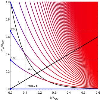
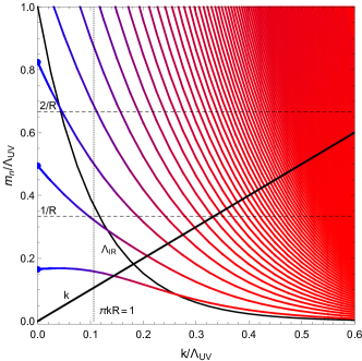
Figure 6: The mass spectrum of the 5D gravity dual of our partially composite DDM theory, plotted as a function of the AdS curvature scale $k$ for two representative choices of $m_{\phi}$. The results shown in the left panel correspond to the choice of $m_{\phi}=10^{-4}\Lambda_{\rm UV}$, while the results shown in the right panel correspond to the choice of $m_{\phi}=\Lambda_{\rm UV}$. In both panels, we have taken $R=3/\Lambda_{\rm UV}$. Each of the solid curves shown in each panel corresponds to a particular value of the index $n$ and indicates the mass $\hat{m}_{n}$ of the corresponding ensemble constituent. Thus, the set of points obtained by taking a vertical “slice” through either panel collectively represent the mass spectrum of the theory for the corresponding value of $k$. The color at any given point along each curve provides information about the extent to which the corresponding state in the partially composite theory in 4D is primarily elementary or composite. In particular, the color indicates the absolute value of the projection coefficient $A^{\prime}_{n}$ at that point, normalized to the absolute value of the projection coefficient $A_{n}^{\prime(k=0)}$ obtained for the same choice of $m_{\phi}$ and $R$, but with $k=0$. A value near $|A^{\prime}_{n}/A_{n}^{\prime(k=0)}|=0$ (red) suggests that the state is primarily composite, while a value near $|A^{\prime}_{n}/A_{n}^{\prime(k=0)}|=1$ (blue) suggests that the state is primarily elementary. Curves indicating the value of $k$ (solid black line with unit slope), $1/R$ and $2/R$ (dashed black horizontal lines), and $\Lambda_{\rm IR}$ (dot-dashed black curve) are also provided for reference.

In order to motivate why this quantity is a useful proxy for compositeness, we note once again that the flat-space limit of the 5D dual theory corresponds to the limit in which all of the states of the corresponding 4D theory are purely elementary. As discussed in Appendix A, the bulk profile of each state in this limit reduces to

$$\hat{\zeta}_{n}^{(k=0)}(y)~{}=~{}\frac{r_{n}}{\sqrt{\pi R}}\cos\left(\frac{n\pi y}{R}\right)~{},$$ (88)

where we have defined

$$r_{n}~{}\equiv~{}\begin{cases}1&n=0\\ \sqrt{2}&n>0~{}.\end{cases}$$ (89)

Using the completeness relation in Eq. (49) for these flat-space bulk profiles with $y^{\prime}=0$, we may express $A^{\prime}_{n}$ for general $k$ in the more revealing form

$$A^{\prime}_{n} = \sqrt{\frac{1-e^{-2\pi kR}}{2k}}\int_{0}^{\pi R}\hat{\zeta}_{n}(y)\delta(y)dy$$

$$= \sqrt{\frac{1-e^{-2\pi kR}}{2k}}\int_{0}^{\pi R}\hat{\zeta}_{n}(y)\sum_{m=0}^{\infty}\frac{r_{m}^{2}}{\pi R}\cos\left(\frac{m\pi y}{R}\right)dy$$

$$= \sqrt{\frac{1-e^{-2\pi kR}}{2\pi kR}}\sum_{m=0}^{\infty}r_{m}\!\!\int_{0}^{\pi R}\!\!\hat{\zeta}_{m}^{(k=0)}(y)\hat{\zeta}_{n}(y)dy~{},$$

where in going from the first to the second line, we have used the completeness relation

$$\sum_{n=0}^{\infty}\hat{\zeta}_{n}^{(k=0)}(y)\hat{\zeta}_{n}^{(k=0)}(y^{\prime})~{}=~{}\delta(y-y^{\prime})~{},$$ (91)

with $y^{\prime}=0$. Thus, up to an overall normalization coefficient and an additional factor of $r_{n}$ which appears in each term of the sum, $A^{\prime}_{n}$ can be viewed as a sum of the overlap integrals between the state $\hat{\chi}_{n}$ within the ensemble and the individual mass-eigenstate fields $\hat{\chi}_{m}^{(k=0)}$ of a theory with $k=0$ and the same values of $m_{\phi}$ and $R$. We choose to normalize this quantity to $A_{n}^{\prime(k=0)}$ because $0\leq|A^{\prime}_{n}/A_{n}^{\prime(k=0)}|\leq 1$, with $|A^{\prime}_{n}/A_{n}^{\prime(k=0)}|=1$ occurring in the $k=0$ limit. A value of $|A^{\prime}_{n}/A_{n}^{\prime(k=0)}|$ near unity therefore suggests that the degree of overlap between $\hat{\chi}_{n}$ and the $\hat{\chi}_{m}^{(k=0)}$ is large and that the corresponding state in the partially composite theory is mostly elementary. By contrast, a value near zero suggests that the degree of overlap is small and that the corresponding state is mostly composite.

The results shown in the left panel of the Fig. 6 are characteristic of the regime in which $m_{\phi}$ is considerably smaller than all of the other relevant scales in the problem. In this regime, for $k=0$, the spectrum consists of one light state $\hat{\chi}_{0}$ with a mass $\hat{m}_{0}\ll 1/R$ and several additional states with masses $\hat{m}_{n}\approx n/R$, all of which are elementary. As $k$ is increased, $\hat{m}_{0}$ remains approximately constant and $\hat{\chi}_{0}$ remains approximately elementary. By contrast, the masses of the additional $\hat{\chi}_{n}$ decrease while the degree of compositeness for each of these states increases. Furthermore, additional $\hat{\chi}_{n}$ whose masses descend from infinity successively appear in the spectrum of the theory below $\Lambda_{\rm UV}$ as $k$ increases. The process continues as $k$ is further increased until we enter the $\pi kR\gg 1$ regime in which the spectrum includes a large number of low-lying states with masses in the range $k\gg\hat{m}_{n}\gtrsim m_{\rm KK}$, all of which exhibit a high degree of compositeness, as expected.

By contrast, the results shown in the right panel of Fig. 6, which are characteristic of the regime in which $m_{\phi}$ is significantly larger than both $k$ and $1/R$, differ from those in the left panel primarily for small $k$. Most notably, the masses of the states obtained for $k=0$ are not given by $\hat{m}_{n}\approx n/R$ as they are in the left panel, but rather by $\hat{m}_{n}\approx(n+\frac{1}{2})/R$. Once again, this accords with the expected behavior of the $\hat{m}_{n}$ in the flat-space limit DDM1 . For larger $k$, the only qualitative difference between the mass spectra obtained in the small-$m_{\phi}$ and large-$m_{\phi}$ regimes is that the spectrum in the latter regime lacks the single, primarily elementary state with $\hat{m}_{0}\ll m_{\rm KK}$ present in the former regime. Indeed, for large $m_{\phi}$, we see that all of the low-lying states within the ensemble are primarily composite when $k$ is large.

VI Conclusions

In this paper, we have investigated a novel realization of the DDM framework within the context of a strongly-coupled CFT. In this scenario, the constituent particles of the DDM ensemble are the composite states which emerge in the spectrum of the theory below the scale at which conformal invariance is spontaneously broken. Abundances and decay widths for these ensemble constituents can be generated through mixing between these composite states and an additional, elementary scalar $\phi_{0}$, yielding a spectrum of partially composite mass-eigenstates whose degree of compositeness varies across the ensemble. Informed by the AdS/CFT correspondence, we have derived the masses, decay widths, and cosmological abundance for these partially composite states within the context of the gravity dual of this scenario — a theory involving a scalar field propagating in the bulk of a slice of AdS₅. We have investigated the extent to which model-independent bounds on the total abundance and the equation of state for the ensemble constrain the parameter space of this scenario, and we have shown that indeed a balancing between decay widths and abundances appropriate for a DDM ensemble arises within large regions of that parameter space, even within the regime wherein the degree of warping in the dual theory is significant — a regime which corresponds to the regime in which there exists a significant hierarchy of scales $\Lambda_{\rm IR}\ll\Lambda_{\rm UV}$ in the partially composite theory. However, we have also shown that constraints on the ensemble become increasingly stringent as the degree of warping increases. Moreover, we have shown that interesting qualitative features, such as non-monotonicities in the spectrum of decay widths, can develop in the highly-warped regime of the dual theory which do not arise in the flat-space limit.

A few comments are in order. First of all, because our primary focus in this paper has been the 4D partially composite DDM scenario, we have regarded the 5D gravity dual of this theory primarily as a calculational tool for obtaining information about the properties of the ensemble in the 4D theory. However, the fact that a viable DDM ensemble can emerge in the context of a scenario involving a warped extra dimension is interesting in its own right. Indeed from this perspective, we may regard the results in Sects. III and IV as generalizations of the flat-space results derived in Refs. DDM1 ; DDM2 to warped space.

On a final note, in constraining the parameter space of our scenario, we have focused on considerations such as limits on $w_{\mathrm{eff}}$ and $\Omega_{\mathrm{tot}}$ in bounding the parameter space of our scenario — considerations which do not depend sensitively on the identities of the final-state particles into which the ensemble constituents decay. If the $\hat{\chi}_{n}$ decay solely into other, lighter particles which reside within the dark sector but are external to the ensemble (e.g., particles which behave as dark radiation rather than dark matter), these constraints are typically the leading ones. By contrast, if the $\hat{\chi}_{n}$ decay into final states involving visible-sector particles, additional constraints apply. It would be interesting to consider how such constraints further restrict the parameter space of our ensemble for certain well-motivated decay scenarios in which decays to SM particles dominate the width of each $\hat{\chi}_{n}$.

Appendix A Mixing and Projection Coefficients in the Flat-Space Limit

In Sect. III, we derived analytic approximations for $A_{n}$ and $A^{\prime}_{n}$ valid within the regime in which $\pi kR\gg 1$ and $k\gg\hat{m}_{n}\gg m_{\rm KK}$. In this Appendix, in order to make contact with the results obtained in Refs. DDGAxion ; DDM1 for the case of a flat extra dimension, we derive the corresponding expressions valid in the regime in which $\hat{m}_{n}\gg k$ and then demonstrate that these expressions reduce to the expected results in the $k\rightarrow 0$ limit.

We begin by considering the mass spectrum of the theory at early times $t\lesssim t_{G}$, before the phase transition occurs. The mass spectrum of the $\chi_{n}$ in this phase of the theory consists of the solutions to Eq. (33). In the regime in which $\pi kR\ll 1$, this equation reduces to

$$\sin\left(\pi m_{n}R\right)~{}\approx~{}0~{},$$ (92)

which implies that $m_{n}\approx n/R$, in accord with the expected flat-space result.

We now consider the mass spectrum of the theory at times $t\gtrsim t_{G}$, after the brane mass has been generated. Since the action in the flat-space limit is symmetric under the coordinate transformation $y\rightarrow\pi R-y$, the mass spectrum of the $\hat{\chi}_{n}$ in this limit is the same regardless of whether the dynamics that generates $m_{\phi}$ is localized on the UV or IR brane. We therefore focus on the case in which this dynamics is localized on the UV brane. The mass spectrum of the $\hat{\chi}_{n}$ in this phase of the theory consists of the solutions to Eq. (41). In the regime in which $\hat{m}_{n}\gg k$, regardless of the value of $\pi kR$, the Bessel functions in this equation are well approximated by

$$J_{\alpha}(x) \approx \sqrt{\frac{2}{\pi x}}\cos\left(x-\frac{\alpha\pi}{2}-\frac{\pi}{4}\right)$$

$$Y_{\alpha}(x) \approx \sqrt{\frac{2}{\pi x}}\sin\left(x-\frac{\alpha\pi}{2}-\frac{\pi}{4}\right)~{}.$$ (93)

One therefore finds that, in this regime, Eq. (41) reduces to

$$\frac{m_{\phi}^{2}}{2k}\left(1-e^{-2\pi kR}\right)\cot\left[\frac{\hat{m}_{n}}{k}\left(e^{\pi kR}-1\right)\right]~{}\approx~{}\hat{m}_{n}~{}.$$ (94)

In the regime in which $\pi kR\ll 1$, this equation further reduces to

$$\pi m_{\phi}^{2}R\cot(\pi\hat{m}_{n}R)~{}\approx~{}\hat{m}_{n}~{}.$$ (95)

This result — and therefore the mass spectrum of the $\hat{\chi}_{n}$ obtained in this regime — agrees with the corresponding flat-space expression in Ref. DDM1 ; DDGAxion . The solutions for $\hat{m}_{n}$ are given by $\hat{m}_{n}\approx(n+\frac{1}{2})/R$ for $n\ll\pi m_{\phi}^{2}R^{2}$ and $\hat{m}_{n}\approx n/R$ for $n\gg\pi m_{\phi}^{2}R^{2}$ and interpolate smoothly between these asymptotic expressions.

In order to derive the corresponding analytic approximations for $A_{n}$ and $A^{\prime}_{n}$, we begin by noting that for $m_{n}\gg k$, the expression for the bulk profile $\zeta_{n}(y)$ of the early-time mass eigenstate $\chi_{n}$ in Eq. (35) reduces to

$$\zeta_{n}(y)~{}\approx~{}\frac{r_{n}}{\sqrt{\pi R}}e^{3ky/2}\cos\left[\frac{m_{n}}{k}(e^{ky}-e^{\pi kR})\right]~{},$$ (96)

where we have defined

$$r_{n}~{}\equiv~{}\sqrt{\frac{4\pi m_{n}R}{\frac{2m_{n}}{k}(e^{\pi kR}-1)+\sin\left[\frac{2m_{n}}{k}(e^{\pi kR}-1)\right]}}~{}.$$ (97)

The expression for the bulk profile $\hat{\zeta}_{n}$ of the late-time mass eigenstate $\hat{\chi}_{n}$ is identical in form to the expression for $\zeta_{n}(y)$ in Eq. (96), but with $\hat{m}_{n}$ in place of $m_{n}$.

In the regime in which $\pi kR\ll 1$, Eq. (96) reduces to

$$\zeta_{n}(y)~{}\approx~{}\frac{r_{n}}{\sqrt{\pi R}}\cos\big{[}m_{n}(y-\pi R)\big{]}~{},$$ (98)

where

$$r_{n}~{}\approx~{}\sqrt{\frac{2}{1+\frac{\sin(2\pi m_{n}R)}{2\pi m_{n}R}}}~{}.$$ (99)

We note that for either $m_{n}\approx n/R$ or $m_{n}\approx(n+\frac{1}{2})/R$ with $n\in\mathbb{Z}$, this quantity is well approximated by

$$r_{n}~{}\approx~{}\begin{cases}1&n~{}=~{}0\\ \sqrt{2}&n~{}>~{}0~{}.\end{cases}$$ (100)

Taking into account the difference in normalization conventions, these results agree with those derived in Ref. DDM1 . Since $A_{n}$ and $A^{\prime}_{n}$ are derived directly from $\zeta_{0}(y)$ the corresponding bulk profile $\hat{\zeta}_{n}(y)$, it therefore follows that the mixing and projection coefficients obtained in the $k\rightarrow 0$ limit of our warped-space scenario reproduce those obtained in Refs. DDGAxion ; DDM1 as well.

Substituting our analytic approximation for $\hat{\zeta}_{n}(y)$ into Eq. (44), we find that the mixing-matrix elements are

$$A_{n} \approx \sqrt{\frac{2k}{1-e^{-2\pi kR}}}\frac{\hat{r}_{n}}{\sqrt{\pi R}}$$

$$\times\int^{\pi R}_{0}e^{-ky/2}\cos\left[\frac{\hat{m}_{n}}{k}(e^{ky}-e^{\pi kR})\right]dy~{},$$

where $\hat{r}_{n}$ is given by Eq. (97), but with $\hat{m}_{n}$ in place of $m_{n}$. In order to simplify this expression further, we observe that the integral over $y$ can be written in terms of the Fresnel integrals

$$C(x) \equiv \int_{0}^{x}\cos\left(\frac{\pi t^{2}}{2}\right)dt$$

$$S(x) \equiv \int_{0}^{x}\sin\left(\frac{\pi t^{2}}{2}\right)dt~{}.$$ (102)

In particular, we find that

$$A_{n} \approx \frac{1}{\sqrt{\hat{m}_{n}R(1-e^{-2\pi kR})}}\left(\frac{4\hat{m}_{n}\hat{r}_{n}}{k}\right)$$

$$\times\Bigg{\{}\sin\left(\textstyle\frac{\hat{m}_{n}}{m_{\rm KK}}\right)\bigg{[}C\left(\textstyle\sqrt{\frac{2\hat{m}_{n}}{\pi m_{\rm KK}}}\right)-C\left(\textstyle\sqrt{\frac{2\hat{m}_{n}}{\pi k}}\right)\bigg{]}$$

$$-\cos\left(\textstyle\frac{\hat{m}_{n}}{m_{\rm KK}}\right)\bigg{[}S\left(\textstyle\sqrt{\frac{2\hat{m}_{n}}{\pi m_{\rm KK}}}\right)-S\left(\textstyle\sqrt{\frac{2\hat{m}_{n}}{\pi k}}\right)\bigg{]}$$

$$+\sqrt{\frac{k}{2\pi\hat{m}_{n}}}\cos\left(\textstyle\frac{\hat{m}_{n}}{m_{\rm KK}}-\frac{\hat{m}_{n}}{k}\right)-\sqrt{\frac{m_{\rm KK}}{2\pi\hat{m}_{n}}}\Bigg{\}}~{}.$$

Since we are working within the regime in which $\hat{m}_{n}\gg k$, we may simplify this expression by making use of the well-known asymptotic expansions for $C(x)$ and $S(x)$. In particular, for large arguments $x\gg 1$, these integrals are well approximated by

$$C(x) \approx \frac{1}{2}+\frac{1}{\pi x}\sin\left(\frac{\pi x^{2}}{2}\right)-\frac{1}{\pi^{2}x^{3}}\cos\left(\frac{\pi x^{2}}{2}\right)$$

$$S(x) \approx \frac{1}{2}-\frac{1}{\pi x}\cos\left(\frac{\pi x^{2}}{2}\right)-\frac{1}{\pi^{2}x^{3}}\sin\left(\frac{\pi x^{2}}{2}\right)~{}.$$

With these approximations, we find that Eq. (LABEL:eq:AnFresnalExpansion) reduces to

$$A_{n}~{}\approx~{}\sqrt{\frac{2k}{\pi\hat{m}_{n}^{2}R(1-e^{-2\pi kR})}}\hat{r}_{n}\sin\left[\frac{\hat{m}_{n}}{k}(e^{\pi kR}-1)\right]~{}.$$ (105)

Using Eq. (94) in order to eliminate the trigonometric functions, we arrive at our final expression for $A_{n}$ in the $\hat{m}_{n}\gg k$ regime. After some algebra, we find that

$$A_{n}~{}\approx~{}\sqrt{\frac{\frac{m_{\phi}^{2}}{\hat{m}_{n}^{2}}\left(\frac{1-e^{-2\pi kR}}{e^{\pi kR}-1}\right)}{\frac{\hat{m}_{n}^{2}}{m_{\phi}^{2}}+\frac{m_{\phi}^{2}}{4k^{2}}(1-e^{-2\pi kR})^{2}+\frac{1-e^{-2\pi kR}}{2(e^{\pi kR}-1)}}}~{}.$$ (106)

We note that for $\pi kR\ll 1$, this expression reduces to

$$A_{n}~{}\approx~{}\frac{\sqrt{2}m_{\phi}}{\hat{m}_{n}}\frac{1}{\sqrt{\frac{\hat{m}_{n}^{2}}{m_{\phi}^{2}}+\pi^{2}m_{\phi}^{2}R^{2}+1}}~{},$$ (107)

which once again agrees with the corresponding result in Refs. DDGAxion ; DDM1 .

The analytic approximation for $A^{\prime}_{n}$ in the $\hat{m}_{n}\gg k$ regime, obtained by substituting Eq. (98) into Eq. (48), is

$$A_{n}^{\prime}~{}\approx~{}\sqrt{\frac{1-e^{-2\pi kR}}{2\pi kR}}\hat{r}_{n}\cos\left[\frac{\hat{m}_{n}}{k}(e^{\pi kR}-1)\right]~{}.$$ (108)

Using Eq. (94) in order to eliminate trigonometric functions, we find that this expression simplifies to

$$A^{\prime}_{n}~{}\approx~{}\sqrt{\frac{\frac{\hat{m}_{n}^{2}}{m_{\phi}^{2}}\left(\frac{1-e^{-2\pi kR}}{e^{\pi kR}-1}\right)}{\frac{\hat{m}_{n}^{2}}{m_{\phi}^{2}}+\frac{m_{\phi}^{2}}{4k^{2}}(1-e^{-2\pi kR})^{2}+\frac{1-e^{-2\pi kR}}{2(e^{\pi kR}-1)}}}~{}.$$ (109)

Comparing this result with Eq. (106), we observe that $A_{n}^{\prime}\approx(\hat{m}_{n}/m_{\phi})^{2}A_{n}$ within this regime, in accord with the relationship between the mixing and projection coefficients obtained in Refs. DDGAxion ; DDM1 . Moreover, we observe that the expression in Eq. (109) increases monotonically with $\hat{m}_{n}$. Thus, in the regime in which the AdS curvature is sufficiently small that the criterion $\hat{m}_{n}\gg k$ is satisfied for all $\hat{\chi}_{n}$ within the ensemble, the $A_{n}^{\prime}$ — and therefore also the decay widths $\Gamma_{n}$ — do not exhibit the non-monotonicities discussed in Sect. IV, which can arise when the ensemble includes states with masses $\hat{m}_{n}\lesssim k$.

Appendix B Alternative Brane-Localization Scenarios

In Sect. III we derived expressions for the mixing and projection coefficients $A_{n}$ and $A_{n}^{\prime}$ for the ensemble constituents for the case in which the dynamics which generates the mass term $m_{\phi}$ and the SM particles into which these ensemble constituents decay are both localized on the UV brane. In this Appendix, we derive the corresponding expression for $A_{n}$ for the case in which the dynamics that generates $m_{\phi}$ is localized on the IR brane and the corresponding expression for $A_{n}^{\prime}$ for the case in which the SM is localized on the IR brane. From these results and those appearing in Eqs. (46) and (48), the scaling exponents $\alpha$ and $\beta$ for all possible combinations of locations for the mass-generating dynamics and the SM can be determined in a straightforward manner.

B.1 Mass-Generating Dynamics on the IR Brane

We begin by deriving the mixing coefficients $A_{n}$ for the case in which the dynamics that generates $m_{\phi}$ is localized on the IR brane. At times $t\lesssim t_{G}$ before the scale at which the mass-generating phase transition occurs, the action is essentially the same as it is in the case in which $m_{\phi}$ is localized on the UV brane. The lightest state is likewise massless, with a profile given by Eq. (32), while the remaining states have masses given by the solutions of Eq. (33) and profiles given by Eqs. (35). However, at times $t\gtrsim t_{G}$, the action in this case is given not by Eq. (39), but rather by

$$\mathcal{S}_{\chi}~{}=~{}-\int d^{5}x\sqrt{-g}\Bigg{[}\frac{1}{2}\partial_{M}\chi\partial^{M}\chi-m_{B}\chi^{2}\delta(y-\pi R)\Bigg{]}~{}.$$ (110)

The masses and bulk profiles of the mass eigenstates $\hat{\chi}_{n}$ can be determined by solving the equation of motion derived from Eq. (110) with the boundary conditions

$$\partial_{y}\chi(x,y)\big{|}_{y=0} = 0$$

$$\left(\partial_{y}-m_{B}\right)\chi(x,y)\big{|}_{y=\pi R} = 0~{}.$$ (111)

In particular, the masses $\hat{m}_{n}$ are the solutions to the equation

$$J_{1}\left(\frac{\hat{m}_{n}}{k}\right)\left[\frac{m_{B}}{\hat{m}_{n}e^{\pi kR}}Y_{2}\left(\frac{\hat{m}_{n}}{m_{\rm KK}}\right)-Y_{1}\left(\frac{\hat{m}_{n}}{m_{\rm KK}}\right)\right]\\ ~{}=~{}Y_{1}\left(\frac{\hat{m}_{n}}{k}\right)\left[\frac{m_{B}}{\hat{m}_{n}e^{\pi kR}}J_{2}\left(\frac{\hat{m}_{n}}{m_{\rm KK}}\right)-J_{1}\left(\frac{\hat{m}_{n}}{m_{\rm KK}}\right)\right]~{},$$ (112)

while the bulk profiles once again take the form

$$\hat{\zeta}_{n}(y)~{}=~{}\hat{\mathcal{N}}_{n}e^{2ky}\left[J_{2}\left(\frac{\hat{m}_{n}}{ke^{-ky}}\right)+\hat{b}_{n}Y_{2}\left(\frac{\hat{m}_{n}}{ke^{-ky}}\right)\right]~{},$$ (113)

where $\hat{\mathcal{N}}_{n}$ is a normalization coefficient. However, due to the difference in boundary conditions in this case relative to the case in which $m_{\phi}$ is localized on the UV brane, the constant $\hat{b}_{n}$ is given not by Eq. (37), but rather by

$$\hat{b}_{n}~{}=~{}-\frac{J_{1}\left(\frac{\hat{m}_{n}}{k}\right)}{Y_{1}\left(\frac{\hat{m}_{n}}{k}\right)}~{}.$$ (114)

For any given choice of $m_{\phi}$, $k$, and $R$, evaluating $A_{n}=U_{n0}$ for the case in which $m_{\phi}$ is localized on the IR brane is simply a matter of substituting the expression for $\hat{\zeta}_{n}(y)$ in Eq. (113) into Eq. (44). However, we note that simple analytic expressions for the $A_{n}$ can be derived within the regime in which $m_{\phi}\ll m_{\rm KK}$. As in the case in which $m_{\phi}$ is localized on the UV brane, we find that $A_{0}$ is approximately unity. Moreover, within the same regime, we find that the mixing coefficients for all $\hat{\chi}_{n}$ with masses within the regime $k\gg\hat{m}_{n}\gg m_{\rm KK}$ are well approximated by

$$A_{n}~{}\approx~{}e^{-3\pi kR}\left(\frac{m_{\phi}}{m_{\text{KK}}}\right)^{2}\left(\frac{m_{\text{KK}}}{\hat{m}_{n}}\right)^{2}~{},$$ (115)

while the $\hat{m}_{n}$ themselves are once again well approximated by the expression in Eq (47).

The initial abundances $\Omega_{n}^{0}$ for the ensemble constituents with masses within the regime $k\gg\hat{m}_{n}\gg m_{\rm KK}$ in the case in which the mass-generating dynamics is localized on the IR brane may be obtained simply by substituting our result for $A_{n}$ in Eq. (115) into Eq. (52). This yields

$$\Omega_{n}^{0}~{}\sim~{}\begin{cases}\hat{m}_{n}^{-2}&\text{instantaneous}\\ \hat{m}_{n}^{-\frac{7}{2}}&\text{staggered (RD era)}\\ \hat{m}_{n}^{-4}&\text{staggered (MD era)}~{}.\\ \end{cases}$$ (116)

B.2 SM on the IR Brane

We have seen in cases in which the SM fields into which the $\hat{\chi}_{n}$ decay are localized on the UV brane, the quantity $A_{n}^{\prime}$ plays a crucial role in determining how $\Gamma_{n}$ scales with $\hat{m}_{n}$ across the ensemble. By contrast, in cases in which the SM fields are localized on the IR brane, it is the quantity $A_{n}^{\prime\prime}$, which describes the projection of $\hat{\chi}_{n}$ onto the IR brane at $y=\pi R$, which plays this same role. In general, these projection coefficients are given by

$$A_{n}^{\prime\prime} \equiv e^{-4\pi kR}\sqrt{\frac{1-e^{-2\pi kR}}{2k}}$$ (117)

$$\times\sum_{\ell=0}^{\infty}\zeta_{\ell}(\pi R)\int_{0}^{\pi R}dy~{}e^{-2ky}\zeta_{\ell}(y)\hat{\zeta}_{n}(y)$$

$$= e^{-4\pi kR}\sqrt{\frac{1-e^{-2\pi kR}}{2k}}\hat{\zeta}_{n}(\pi R)~{},$$

where in going from the first to the second line, we have once again used the completeness relation in Eq. (49).

As was the case with our expression for $A^{\prime}_{n}$ in Eq. (48), the expression for $A_{n}^{\prime\prime}$ in Eq. (117) turns out to have a simple analytic form within the regime in which $m_{\phi}\ll m_{\rm KK}$ and $k\gg\hat{m}_{n}\gtrsim m_{\rm KK}$. In particular, we find that

$$A_{n}^{\prime\prime}~{}\approx~{}e^{-3\pi kR}~{}.$$ (118)

The scaling relation for the decay widths in this regime may be obtained by substituting this result for $A^{\prime\prime}_{n}$ into Eq. (62), which yields

$$\Gamma_{n}~{}\propto~{}\hat{m}_{n}^{3}~{}.$$ (119)

The density of states per unit $\Gamma$ in this case is therefore

$$n_{\Gamma}~{}\sim~{}n_{m}(\Gamma)\left(\frac{d\Gamma}{dm}\right)^{-1}~{}\sim~{}\Gamma^{-2/3}.$$ (120)

Given these results above and the results in Sect. IV, it is straightforward to evaluate the values of $\alpha$ and $\beta$ obtained in the $\hat{m}_{n}\ll m_{\rm KK}$ regime for any of the four possible configurations for the brane mass and the SM fields. These values are tabulated in Table 1.

References

- (1) K. R. Dienes and B. Thomas, Phys. Rev. D 85, 083523 (2012) [arXiv:1106.4546 [hep-ph]].
- (2) K. R. Dienes and B. Thomas, Phys. Rev. D 85, 083524 (2012) [arXiv:1107.0721 [hep-ph]].
- (3) K. R. Dienes, E. Dudas and T. Gherghetta, Phys. Rev. D 62, 105023 (2000) [hep-ph/9912455].
- (4) K. R. Dienes and B. Thomas, Phys. Rev. D 86, 055013 (2012) [arXiv:1203.1923 [hep-ph]].
- (5) K. R. Dienes, J. Fennick, J. Kumar and B. Thomas, Phys. Rev. D 93, no. 8, 083506 (2016) [arXiv:1601.05094 [hep-ph]].
- (6) K. R. Dienes, F. Huang, S. Su and B. Thomas, Phys. Rev. D 95, no. 4, 043526 (2017) [arXiv:1610.04112 [hep-ph]].
- (7) K. R. Dienes, F. Huang, S. Su and B. Thomas, PoS Confinement 2018, 008 (2018).
- (8) J. M. Maldacena, Int. J. Theor. Phys. 38, 1113 (1999) [Adv. Theor. Math. Phys. 2, 231 (1998)] [hep-th/9711200].
- (9) S. S. Gubser, I. R. Klebanov and A. M. Polyakov, Phys. Lett. B 428, 105 (1998) [hep-th/9802109].
- (10) E. Witten, Adv. Theor. Math. Phys. 2, 253 (1998) [hep-th/9802150].
- (11) J. E. Kim, Phys. Rev. D 31, 1733 (1985).
- (12) R. Contino and A. Pomarol, JHEP 0411, 058 (2004) [hep-th/0406257].
- (13) E. Witten, Nucl. Phys. B 160, 57 (1979).
- (14) L. Randall and R. Sundrum, Phys. Rev. Lett. 83, 3370 (1999) [hep-ph/9905221].
- (15) I. R. Klebanov and E. Witten, Nucl. Phys. B 556, 89 (1999) [hep-th/9905104].
- (16) T. Gherghetta and A. Pomarol, Nucl. Phys. B 586, 141 (2000) [hep-ph/0003129].
- (17) B. Batell and T. Gherghetta, Phys. Rev. D 76, 045017 (2007) [arXiv:0706.0890 [hep-th]].
- (18) K. R. Dienes, J. Fennick, J. Kumar and B. Thomas, Phys. Rev. D 97, no. 6, 063522 (2018) [arXiv:1712.09919 [hep-ph]].