A SPECTRAL ANALYSIS OF $FERMI$-LLE GRBs

Abstract

The prompt emission of gamma-ray bursts remains mysterious since the mechanism is difficult to understand even though there are much more observations with the development of detection technology. But most of the gamma-ray bursts spectra show the Band shape, which consists of the low energy spectral index $\alpha$, the high energy spectral index $\beta$, the peak energy $E_{p}$ and the normalization of the spectrum. We present a systematic analysis of the spectral properties of 36 GRBs, which were detected by the Gamma-ray Burst Monitor (GBM), simultaneously, were also observed by the Large Area Telescope (LAT) and the LAT Low Energy (LLE) detector on the $Fermi$ satellite. We performed the detailed time-resolved spectral analysis for all of the bursts in our sample. We found that the time-resolved spectrum at peak flux can be well fitted by the empirical Band function for each burst in our sample. Moreover, the evolution patterns of $\alpha$ and $E_{p}$ have been carried for statistical analysis, and the parameter correlations have been obtained such as $E_{p}-F$, $\alpha-F$, and $E_{p}-\alpha$, all of them are presented by performing the detailed time-resolved spectral analysis. We also demonstrated that the two strong positive correlations $\alpha-F$ and $E_{p}-\alpha$ for some bursts originate from a non-physical selection effects through simulation.

1 Introduction

As we all know, gamma-ray bursts (GRBs) are the brightest explosions in the universe. generally believed that they are from the magnetars or black holes the mergers of compact binaries (NS-NS or BH-NS) or the death of massive stars (Colgate, 1974; Paczynski, 1986; Eichler et al., 1989; Narayan et al., 1992; Woosley, 1993; MacFadyen & Woosley, 1999; Woosley & Bloom, 2006; Kumar & Zhang, 2015). The Band function (Band et al., 1993) can fit the gamma-ray burst spectra such as the time-integrated spectra and the time-resolved spectra, which is contained four parameters, the index $\alpha$, the high energy index $\beta$, the peak energy $E_{p}$ and the normalized constant. It is proved that these parameters with time instead of remaining constant. Many , such as Golenetskii et al. (1983), Norris et al. (1986), Kargatis et al. (1994), Bhat et al. (1994), Ford et al. (1995), Crider et al. (1997), Kaneko et al. (2006), Peng et al. (2009) in pre-$Fermi$ era and Lu et al. (2012), Yu et al. (2016), Acuner & Ryde (2018), Li (2019), Yu et al. (2019) in $Fermi$ era have shown the characteristics of $\alpha$ and $E_{p}$ in Band function (Band et al., 1993). There are three types for the evolution patterns of peak energy $E_{p}$, (i) ‘hard-to-soft’ trend, the value of $E_{p}$ is decreasing monotonically(Norris et al., 1986; Bhat et al., 1994; Band, 1997); (ii) with flux, i.e., $E_{p}$ will be increasing/decreasing since the flux is increasing/decreasing, named ‘flux-tracking’ trend (Golenetskii et al., 1983; Ryde & Svensson, 1999); (iii) ‘soft-to-hard’ trend or chaotic evolutions (Laros et al., 1985; Kargatis et al., 1994). Recently, Lu et al. (2012) and Yu et al. (2019) pointed out that the first two patterns are dominated. the low energy photon index $\alpha$, it does not show strong general trend compared with $E_{p}$ although it evolves with time instead of remaining constant. However, . On the other hand, analysis of a large sample of GRBs for the parameters evolution and the parameter correlations , except for the single burst analysis, such as GRB 131231A in Li et al. (2019) which is a single-pulse burst, and GRB 180720B which is a multi-peaked burst in prompt light curve.

the launch of Fermi Space Gamma-ray Telescope in 2008 (Atwood et al., 2009) it possible to detect GRBs in broad energy both in prompt emission and afterglow phase. $Fermi$ satellite consists of the Gamma-ray Burst Monitor (GBM) and Large Area Telescope (LAT) with the LAT Low Energy (LLE) detector. The GBM consists of 12 NaI detectors (8 to 900 keV) and 2 BGO (200 keV to 40 MeV) detectors. the energy range in GBM detection is from 8 keV to 40 MeV. The LAT can detect the photons with energy range from 100 MeV to 300 GeV. Moreover, the LLE can collect those lower energy gamma-ray photons down to 10 MeV. 2000 GRBs detected by $Fermi$ in the last ten years while the fewer of them were detected by $Fermi$-LAT, which is the number with value of more than one hundred. the GRBs with the detection of LLE are less than one hundred according to the available data at the Fermi Science Support Center (FSSC). The photons 8 orders of magnitude for LLE bursts.

In this work, after performing the detailed time-resolved spectral analysis of the bright gamma-ray bursts with the detection of $Fermi$-LLE in prompt phase, Then we give the evolution patterns the peak energy $E_{p}$ and spectral index $\alpha$. parameter correlations be presented in our analysis such as $E_{p}-F$, $\alpha-F$, and $E_{p}-\alpha$. we make statistical analysis for whether the indices $\alpha$ exceed the synchrotron given by Preece et al. (1998) in these slices.

2 sample selection and method

Up to now, more than one hundred bursts have been co-detected by the $Fermi$/GBM and LAT. were also detected by LLE which can collect those lower energy gamma-ray photons down to 10 MeV in all of these bursts if there is no omission in our collection. This work makes use of all available LLE bursts observed until 20 July 2018. We remove a pure black body burst GRB 090902B, three extremely bright bursts () and 2 long bursts that have been studied in Li et al. (2019) (GRB 131231A) and (GRB 180720B) in detail. are originated from synchrotron emission in prompt phase.

We download data from the FSSC described as above. To complete this study, we take RMFIT as the tool of making time-resolved spectral analysis. We perform the detailed time-resolved spectral analysis by using the TTE event data files of two NaI detectors and the corresponding BGO detector(s) on $Fermi$/GBM, but because of lower impact for peak energy $E_{p}$ and low energy spectral index $\alpha$. background photon counts were estimated by fitting the light curve before and after the operated burst with a one-order background polynomial model. We selected all of the prompt phase as the source. We take the signal-to-noise ratio (S/N) as 40 in all of the slices for each burst and they all can be well fitted by Band function (Band et al., 1993). show the spectral evolution, the sample in our analysis includes only those bursts which at least five time-resolved spectra can be produced from the data. Based on this, GRBs have been excluded due to the insufficiency of the number of time-resolved spectra. by filtering described as above. The reduced $\chi^{2}$ has been taken into measuring the goodness-of-fit. The $\chi^{2}/dof$ is typically in the range of 0.75-1.5 in each slice.

For the evolution patterns of $\alpha$ and $E_{p}$, we will identify them as ‘hard-to-soft’ (h.t.s.), ‘soft-to-hard’ (s.t.h.), ‘intensity-tracking’ (i.t.), ‘rough-tracking’ (r.t.), ‘anti-tracking’ (a.t.) and ‘no’ which means that it evolves without rule. all ‘-tracking’ patterns based on the evolution of energy flux. the statistical analysis of the linear dependence in the parameter correlations such as $E_{p}-F$, $\alpha-F$, and $E_{p}-\alpha$ will be made by using Pearson’s correlation coefficient r.

3 data analysis and results

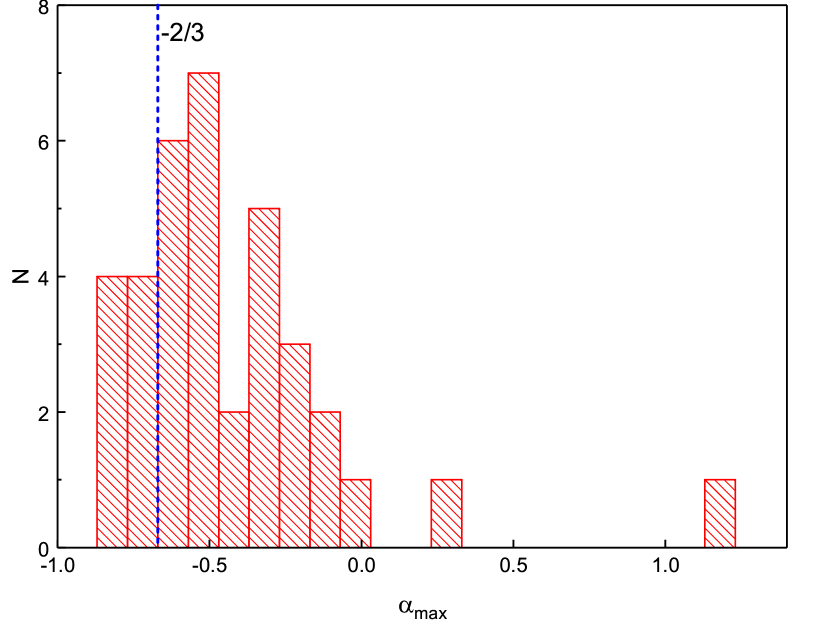
Figure 1: The histogram of the maximal value of $\alpha$ in the detailed time-resolved spectra for each burst. The blue short dash line indicates the synchrotron limit ($-\frac{2}{3}$). of the bursts have an $\alpha_{max}$ which is larger than the synchrotron limit in our sample of bursts.

3.1 Band-fitting Results at Peak Flux for All of the Bursts

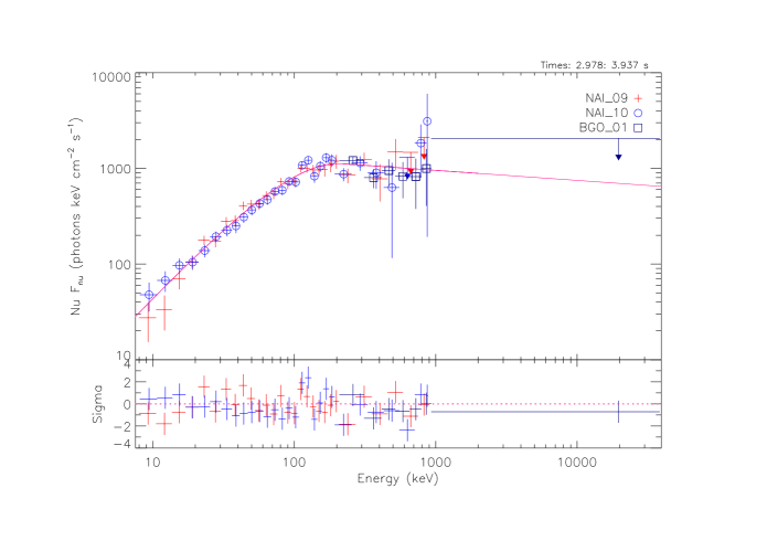
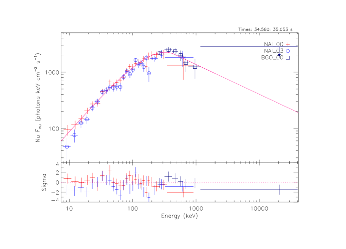
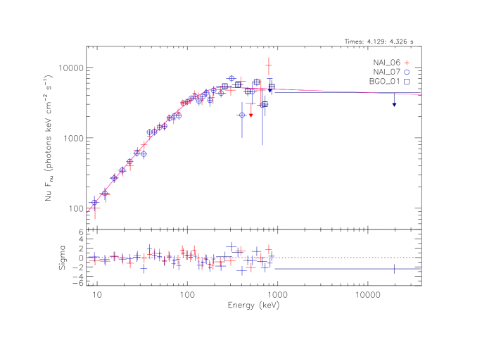
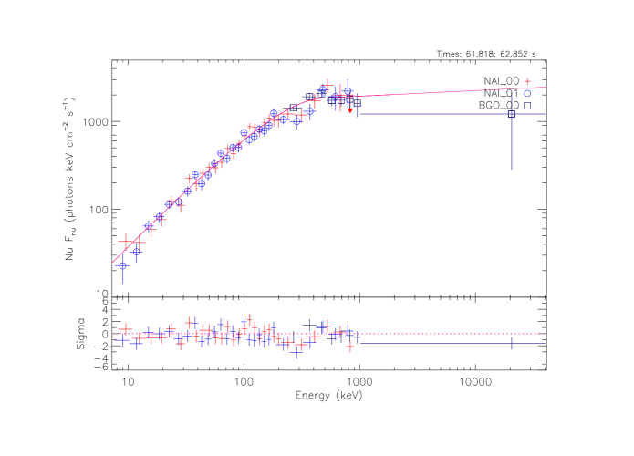
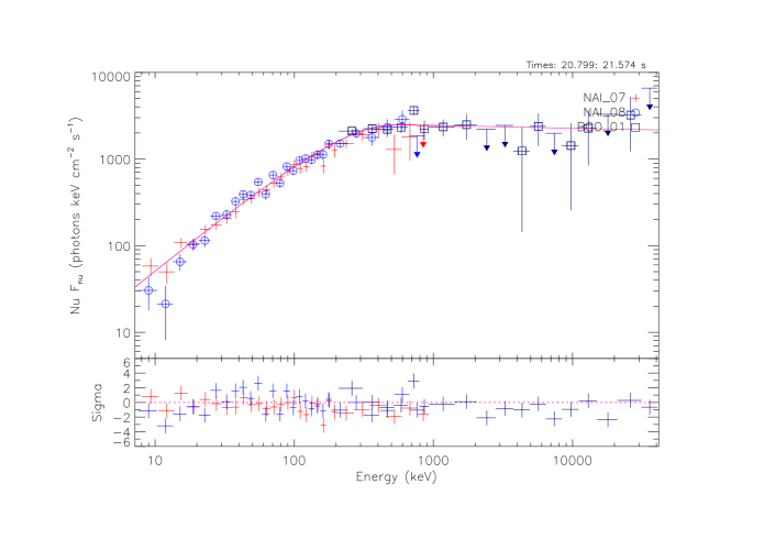
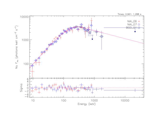
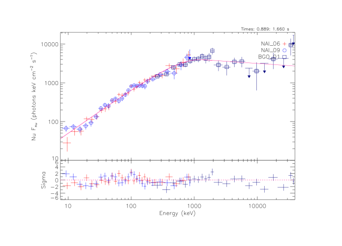
Figure 2:

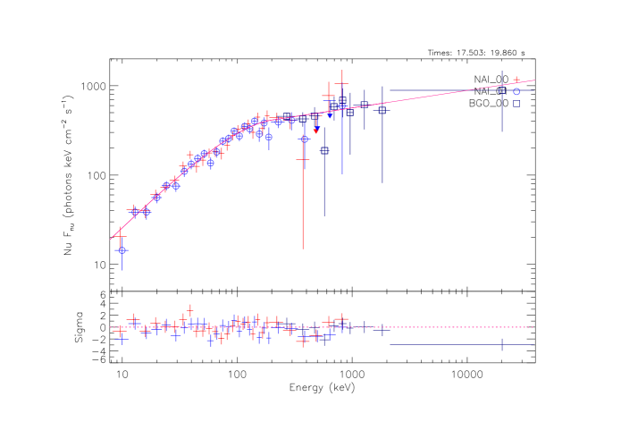
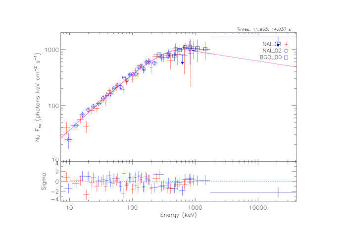
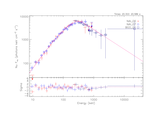
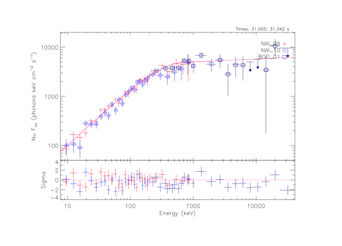
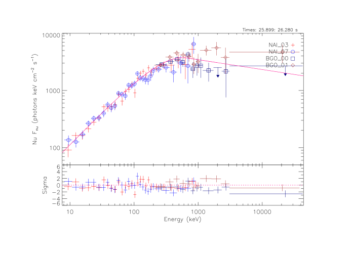
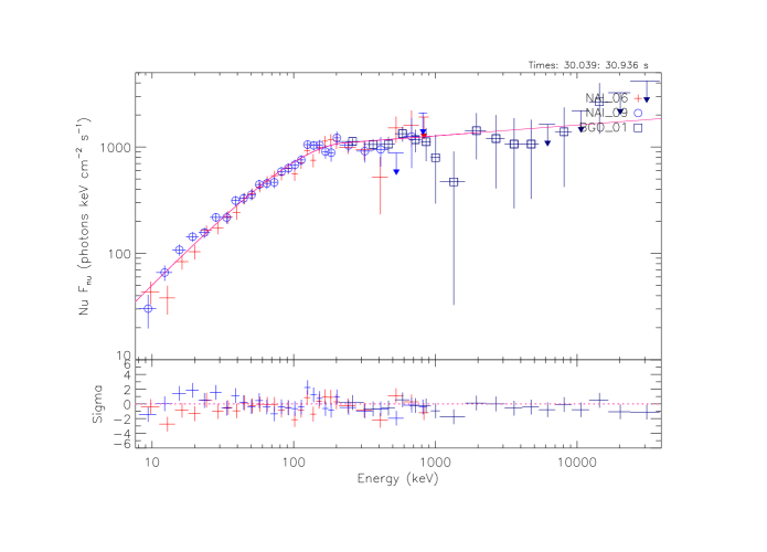
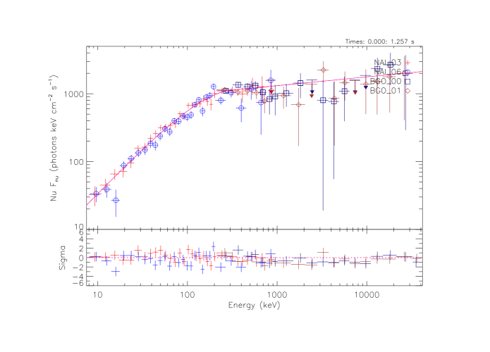
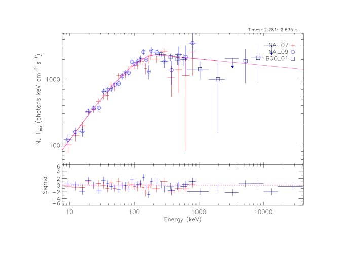
Figure 2: -continued

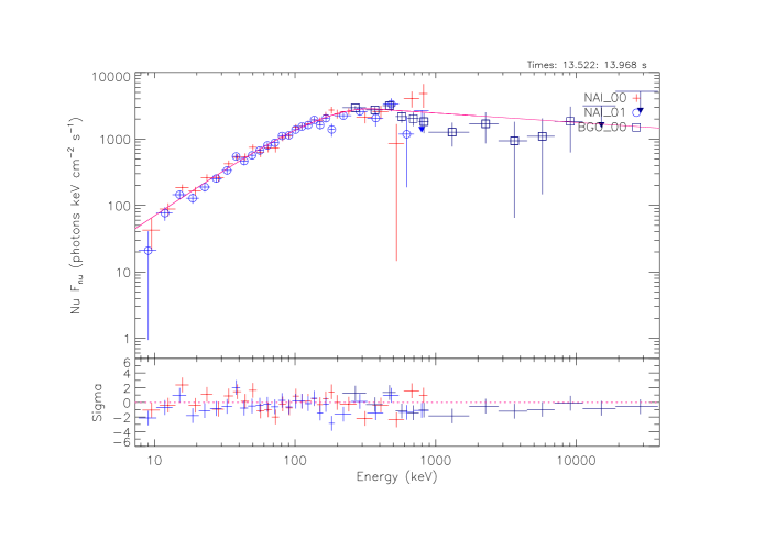
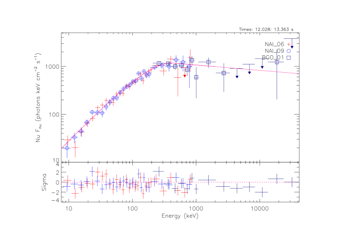
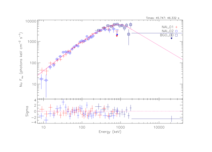
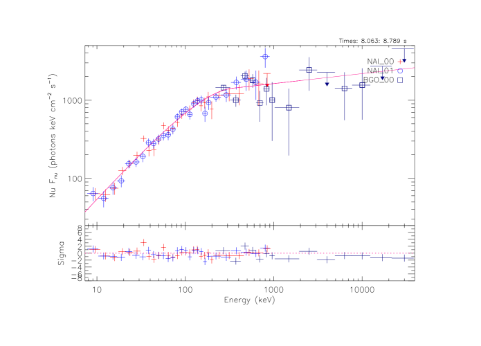
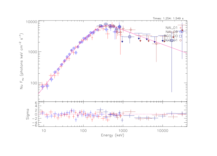
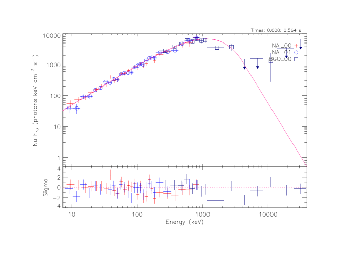
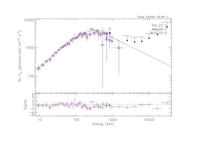
Figure 2: -continued

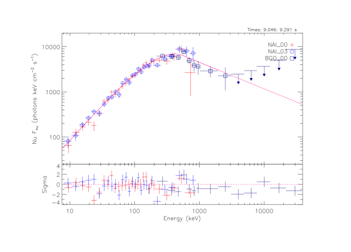
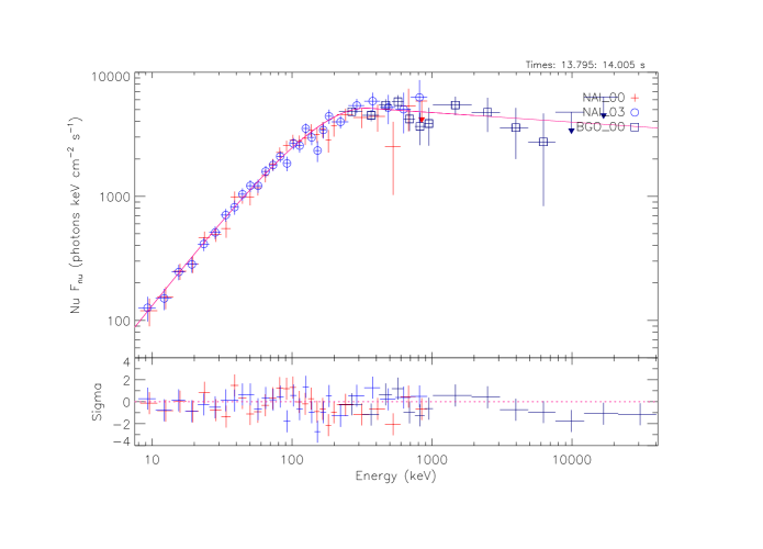
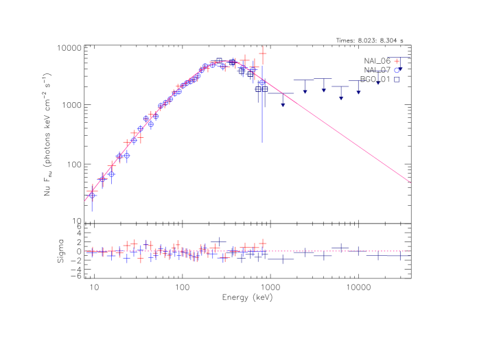
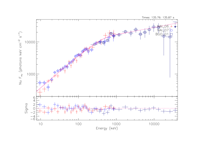
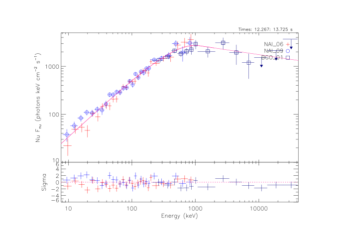
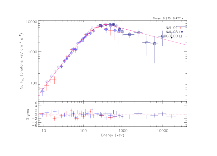
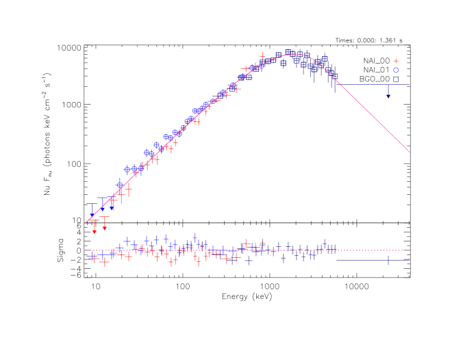
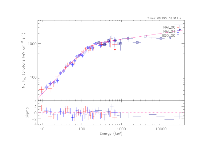
Figure 2: -continued

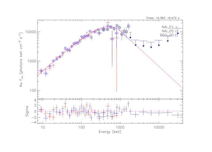
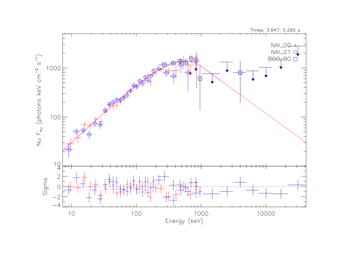
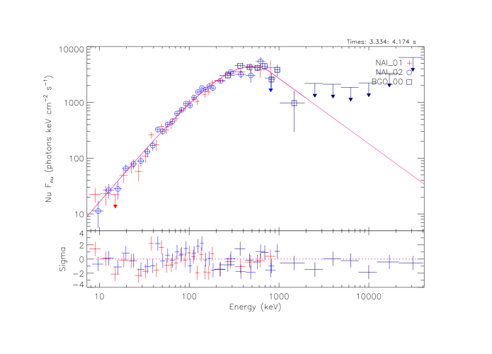
Figure 2: -continued

Table 1: Results of the Time-resolved Spectral Fits at Peak Flux for All Samples

GRB	$t_{1}\sim t_{2}$	$\alpha$	$\beta$	$E_{p}$	Red.$\chi^{2}$
	(s)			(keV)
080825C	2.978$\sim$3.937	-0.4269$\pm$0.0924	-2.105$\pm$0.102	205.1$\pm$19.5	0.96
090328A	23.705$\sim$25.400	-0.9062$\pm$0.0500	-2.220$\pm$0.192	444.0$\pm$57.2	1.15
090626A	34.580$\sim$35.053	-0.7057$\pm$0.0541	-2.530$\pm$0.239	324.7$\pm$27.3	0.92
090926A	4.129$\sim$4.326	-0.3629$\pm$0.0699	-2.048$\pm$0.055	249.5$\pm$18.7	0.97
100724B	61.818$\sim$62.852	-0.6834$\pm$0.0469	-1.936$\pm$0.060	517.2$\pm$52.6	1.09
100826A	20.799$\sim$21.574	-0.7023$\pm$0.0461	-2.033$\pm$0.072	536.0$\pm$53.3	1.12
101014A	0.961$\sim$1.288	-0.4757$\pm$0.0542	-2.334$\pm$0.101	281.6$\pm$18.0	1.02
110721A	0.889$\sim$1.660	-0.8542$\pm$0.0321	-2.111$\pm$0.095	1236.0$\pm$145	1.18
120226A	17.503$\sim$19.860	-0.7359$\pm$0.0857	-1.805$\pm$0.063	238.4$\pm$37.3	1.04
120624B	11.963$\sim$14.037	-0.9411$\pm$0.0443	-2.174$\pm$0.172	611.3$\pm$85.0	0.88
130502B	20.322$\sim$20.586	-0.1871$\pm$0.0530	-2.829$\pm$0.199	320.3$\pm$15.0	0.95
130504C	31.005$\sim$31.342	-0.8189$\pm$0.0500	-1.938$\pm$0.070	705.9$\pm$97.9	1.00
130518A	25.899$\sim$26.280	-0.8515$\pm$0.0394	-2.172$\pm$0.075	567.6$\pm$51.3	0.97
130821A	30.039$\sim$30.936	-0.6272$\pm$0.0733	-1.898$\pm$0.055	246.9$\pm$27.3	0.99
131108A	0.000$\sim$1.257	-0.6219$\pm$0.0672	-1.871$\pm$0.040	341.0$\pm$34.6	0.98
140102A	2.281$\sim$2.635	-0.6150$\pm$0.0710	-2.099$\pm$0.075	223.4$\pm$20.5	0.93
140206B	13.522$\sim$13.968	-0.5438$\pm$0.0569	-2.142$\pm$0.079	336.6$\pm$26.7	1.02
141028A	12.028$\sim$13.363	-0.6414$\pm$0.0555	-2.111$\pm$0.103	416.2$\pm$40.0	0.97
150118B	45.747$\sim$46.332	-0.5728$\pm$0.0329	-3.067$\pm$0.316	881.3$\pm$53.4	0.96
150202B	8.063$\sim$8.789	-0.7736$\pm$0.0612	-1.872$\pm$0.070	383.2$\pm$53.8	1.07
150314A	1.254$\sim$1.549	-0.3399$\pm$0.0448	-2.462$\pm$0.088	413.5$\pm$19.8	1.03
150403A	10.798$\sim$11.410	-0.6775$\pm$0.0418	-2.059$\pm$0.074	639.9$\pm$59.6	1.11
150510A	0.000$\sim$0.564	-0.6889$\pm$0.0275	unconstrained	1141.0$\pm$65.9	0.97
150627A	59.694$\sim$59.961	-0.8258$\pm$0.0441	-2.627$\pm$0.228	317.8$\pm$24.3	0.87
150902A	9.046$\sim$9.291	-0.3920$\pm$0.0471	-2.587$\pm$0.142	411.5$\pm$22.7	0.98
160509A	13.795$\sim$14.005	-0.5605$\pm$0.0573	-2.077$\pm$0.069	336.7$\pm$28.7	0.91
160816A	8.023$\sim$8.304	-0.0321$\pm$0.0625	-3.032$\pm$0.287	322.8$\pm$15.0	0.91
160821A	135.76$\sim$135.87	-0.9698$\pm$0.0376	-1.776$\pm$0.054	1093.0$\pm$192.0	1.12
160905A	12.267$\sim$13.725	-0.7799$\pm$0.0423	-2.197$\pm$0.113	987.2$\pm$120.0	1.15
160910A	8.235$\sim$8.477	-0.2183$\pm$0.0540	-2.332$\pm$0.072	370.8$\pm$19.8	0.94
170115B	0.000$\sim$1.361	-0.5548$\pm$0.0284	-3.430$\pm$0.423	1931.0$\pm$102.0	1.04
170214A	60.990$\sim$62.311	-0.6362$\pm$0.0650	-1.821$\pm$0.050	360.1$\pm$41.8	0.96
170510A	17.310$\sim$19.347	-0.8697$\pm$0.0543	-2.052$\pm$0.121	433.2$\pm$57.5	0.91
170808B	16.383$\sim$16.472	-0.8287$\pm$0.0341	-3.215$\pm$0.447	514.0$\pm$33.0	0.91
171210A	3.647$\sim$5.265	-0.7582$\pm$0.0415	-2.960$\pm$0.658	572.5$\pm$49.8	0.96
180305A	3.334$\sim$4.174	-0.0916$\pm$0.0525	-3.172$\pm$0.461	502.8$\pm$24.1	1.00

Figure 3:

3.2 Evolution Patterns of $E_{p}$ and $\alpha$

In this section, we give the spectral analysis results which include the time-integrated spectral results and the time-resolved spectral results. Table 2 shows the results of the time-integrated spectral fits for all samples. Figure 6 shows the spectral evolutions for all of the bursts in our sample. The histograms of $E_{p}$ and $\alpha$ obtained by performing the detailed time-resolved spectral analysis have been shown in Figure 7.

3.2.1 The Time-integrated Spectral Results

Table 2: Results of the Time-integrated Spectral Fits for All Samples

GRB	z	$T_{90}$	$t_{1}\sim t_{2}$	$\alpha$	$\beta$	$E_{p}$	Red.$\chi^{2}$
		(s)	(s)			(keV)
080825C	…	22	0$\sim$30.016	-0.6197$\pm$0.0595	-2.243$\pm$0.119	174.7$\pm$11.6	1.14
090328A	0.736	80	0$\sim$80.064	-1.1790$\pm$0.0294	-2.352$\pm$0.366	756.0$\pm$121.0	1.19
090626A	…	70	0$\sim$70.016	-1.1920$\pm$0.0448	-2.061$\pm$0.074	152.2$\pm$15.8	1.10
090926A	2.106	20	0$\sim$25.024	-0.7967$\pm$0.0108	-2.428$\pm$0.054	312.4$\pm$6.1	1.97
100724B	…	111.6	0$\sim$100.031	-0.7046$\pm$0.0251	-1.904$\pm$0.035	384.6$\pm$19.3	1.38
100826A	…	100	0$\sim$100.032	-0.8828$\pm$0.0224	-1.897$\pm$0.029	289.4$\pm$14.4	2.03
101014A	…	450	0$\sim$50.047	-1.1690$\pm$0.0190	-2.470$\pm$0.128	186.7$\pm$8.1	1.46
110721A	0.382	24.45	0$\sim$30.015	-1.0790$\pm$0.0343	-1.742$\pm$0.035	411.1$\pm$56.3	1.10
120226A	…	57	0$\sim$60.032	-0.9439$\pm$0.0390	-2.008$\pm$0.090	266.1$\pm$25.1	1.27
120624B	2.20	271	0$\sim$30.016	-0.9902$\pm$0.0328	-2.505$\pm$0.383	685.4$\pm$78.3	1.13
130502B	…	24	0$\sim$35.006	-0.6279$\pm$0.0129	-2.404$\pm$0.051	303.8$\pm$5.9	1.83
130504C	…	74	0$\sim$80.064	-1.2830$\pm$0.0114	-2.250$\pm$0.110	858.8$\pm$66.4	1.45
130518A	2.49	48	0$\sim$50.045	-0.8689$\pm$0.0157	-2.288$\pm$0.055	408.5$\pm$13.5	1.38
130821A	…	84	0$\sim$100.031	-1.1860$\pm$0.0226	-2.044$\pm$0.073	317.3$\pm$26.4	1.78
131108A	2.4	19	0$\sim$25.024	-0.9453$\pm$0.0253	-2.337$\pm$0.104	381.0$\pm$20.6	1.07
140102A	…	65	0$\sim$30.015	-1.2550$\pm$0.0300	unconstrained	211.2$\pm$13.2	1.21
140206B	…	120	0$\sim$55.039	-1.0260$\pm$0.0158	-2.041$\pm$0.032	271.9$\pm$10.6	2.11
141028A	2.332	31.5	0$\sim$35.008	-0.6429$\pm$0.0415	-1.884$\pm$0.037	254.9$\pm$16.0	1.16
150118B	…	40	0$\sim$50.048	-0.8896$\pm$0.0098	-3.435$\pm$0.439	743.1$\pm$20.5	1.42
150202B	…	167	0$\sim$50.048	-0.7537$\pm$0.0440	-2.260$\pm$0.166	235.0$\pm$17.7	1.23
150314A	1.758	14.79	0$\sim$20.032	-0.8268$\pm$0.0104	-2.897$\pm$0.136	404.7$\pm$7.9	1.55
150403A	2.06	40.9	0$\sim$50.046	-0.7383$\pm$0.0266	-1.986$\pm$0.044	312.8$\pm$15.6	1.18
150510A	…	52	0$\sim$60.032	-1.0530$\pm$0.0104	unconstrained	1640.0$\pm$82.4	1.27
150627A	…	65	0$\sim$80.063	-1.0660$\pm$0.0104	-2.154$\pm$0.030	239.4$\pm$6.1	2.49
150902A	…	14	0$\sim$20.032	-0.7066$\pm$0.0125	-2.480$\pm$0.063	431.9$\pm$9.5	1.62
160509A	1.17	371	0$\sim$50.047	-0.8953$\pm$0.0107	-2.041$\pm$0.024	373.2$\pm$9.8	1.92
160816A	…	14	0$\sim$20.032	-0.7409$\pm$0.0215	-3.350$\pm$0.492	235.8$\pm$6.7	1.14
160821A	…	120	109.952$\sim$170.048	-1.0680$\pm$0.0034	-2.299$\pm$0.021	966.3$\pm$14.9	…
160905A	…	64	0$\sim$80.064	-1.0950$\pm$0.0174	-2.844$\pm$0.359	1392.0$\pm$143.0	1.82
160910A	…	24.3	0$\sim$30.016	-0.9891$\pm$0.0126	-1.776$\pm$0.012	506.9$\pm$22.2	3.86
170115B	…	44	0$\sim$50.048	-0.8061$\pm$0.0239	-2.504$\pm$0.156	997.4$\pm$65.6	2.39
170214A	2.53	123	0$\sim$150.016	-0.9511$\pm$0.0133	-2.519$\pm$0.137	465.7$\pm$16.1	2.03
170510A	…	128	0$\sim$135.040	-1.2760$\pm$0.0315	unconstrained	563.2$\pm$84.9	1.47
170808B	…	17.7	0$\sim$25.024	-0.9949$\pm$0.0101	-2.297$\pm$0.035	249.1$\pm$5.2	2.28
171210A	…	143	0$\sim$145.024	-0.7107$\pm$0.0383	-2.244$\pm$0.063	136.3$\pm$5.6	1.30
180305A	…	12.5	0$\sim$15.040	-0.3126$\pm$0.0266	-2.490$\pm$0.098	329.5$\pm$9.6	1.27

Table 2 shows the results of the time-integrated spectral fits for all samples. Listed in this Table are the GRBs in our sample which satisfy our criteria in this study (Col.1), the redshift of them (Col.2), the duration interval of $T_{90}$ (Col.3), the integrated range in our analysis (Col.4), the low energy photon index $\alpha$ in time-integrated analysis (Col.5), the high energy photon index $\beta$ in time-integrated analysis (Col.6), the peak energy in time-integrated analysis (Col.7) and reduced $\chi^{2}$ (Col.8).

There are GRBs with known redshift. The duration values of $T_{90}$ for most of them in our sample seem to be from 20 s to 100 s. for the time-integrated based on the statistical study such as Preece et al. (2000), Kaneko et al. (2006), Zhang et al. (2011), Goldstein et al. (2012), and Geng & Huang (2013). While the typical value of $\alpha$ in our sample is obtained from Table 2, which is larger than the statistical study of large sample of GRBs, the $E_{p}$ is similar to the previous statistics. time-integrated values of $\alpha$, in GRB 080825C ($\sim-0.6197$), , GRB 141028A ($\sim-0.6429$), violate the synchrotron limit.

Figure 4:

Figure 5:

3.2.2 The Time-resolved Spectral Results

Table 3: Fitting Results of the Parameter Correlations and the Spectral Evolutions of $E_{p}$ and $\alpha$

GRB	Detectors	N	$E_{p}-F$	$\alpha-F$	$E_{p}-\alpha$	Spectral Evolutions	$\alpha>-\frac{2}{3}$	$\alpha-F$	$E_{p}-\alpha$
			r	r	r	$E_{p}/\alpha$		r(S)	r(S)
080825C	n9,na,b1	8	0.94	0.70	0.54	h.t.s./r.t.	yes	-0.38	-0.96
090328A	n7,n8,b1	8	0.70	0.93	0.83	h.t.s./i.t.	no	-0.20	-0.86
090626A	n0,n3,b0	20	0.61	0.69	0.01	r.t./r.t.	not all	-0.56	-0.88
090926A	n6,n7,b1	37	0.61	0.67	0.35	r.t./r.t.	not all	-0.36	-0.86
100724B	n0,n1,b0	30	0.59	0.35	-0.08	r.t./r.t.	not all	…	…
100826A	n7,n8,b1	24	0.93	0.08	-0.01	r.t./r.t.	not all	…	…
101014A	n6,n7,b1	21	0.86	0.83	0.62	r.t./r.t.	not all	0.28	-0.54
110721A	n6,n9,b1	7	0.62	0.76	0.07	h.t.s./s.t.h. to h.t.s.	no	-0.71	-0.88
120226A	n0,n1,b0	12	0.47	0.73	-0.11	r.t./r.t.	no	-0.57	-0.87
120624B	n1,n2,b0	5	0.52	0.61	0.94	h.t.s./h.t.s.	no	-0.40	-0.80
130502B	n6,n7,b1	25	0.64	0.75	0.24	r.t./r.t.	not all	-0.13	-0.67
130504C	n9,na,b1	29	0.54	0.45	-0.18	r.t./r.t.	no	…	…
130518A	n3,n7,b0,b1	19	0.61	0.69	0.32	r.t./r.t.	no	-0.71	-0.81
130821A	n6,n9,b1	11	0.67	0.71	-0.06	r.t./r.t.	not all	-0.002	-0.95
131108A	n3,n6,b0,b1	6	0.84	0.77	0.44	s.t.h. to h.t.s./r.t.	not all	-0.14	-0.32
140102A	n7,n9,b1	6	0.89	0.84	0.71	i.t./i.t.	not all	-0.002	-0.93
140206B	n0,n1,b0	23	0.67	0.58	0.38	r.t./r.t.	not all	…	…
141028A	n6,n9,b1	5	0.91	-0.07	0.18	i.t./h.t.s.	yes	…	…
150118B	n1,n2,b0	20	0.86	0.50	0.26	r.t./r.t.	not all	…	…
150202B	n0,n1,b0	7	0.72	-0.48	-0.69	r.t./a.t.	not all	…	…
150314A	n1,n9,b0,b1	17	0.05	0.95	0.05	no/r.t.	not all	-0.64	-0.89
150403A	n3,n4,b0	9	0.83	0.39	0.01	r.t./r.t.	not all	…	…
150510A	n0,n1,b0	11	0.56	0.95	0.55	s.t.h. to h.t.s./r.t.+h.t.s.	not all	0.27	-0.86
150627A	n3,n4,b0	39	0.66	0.75	0.59	r.t./r.t.	not all	-0.45	-0.79
150902A	n0,n3,b0	17	0.58	0.85	0.29	r.t./r.t.	not all	-0.68	-0.91
160509A	n0,n3,b0	39	0.46	0.83	0.39	r.t./r.t.	not all	-0.18	-0.96
160816A	n6,n7,b1	10	0.76	0.70	0.27	i.t./r.t.	not all	-0.08	-0.64
160821A	n6,n7,b1	130	0.43	0.81	0.08	r.t./r.t.	no	0.07	-0.72
160905A	n6,n9,b1	12	0.71	0.97	0.73	r.t./r.t.	no	0.65	-0.76
160910A	n1,n5,b0	13	0.83	0.17	-0.06	h.t.s./no	not all	…	…
170115B	n0,n1,b0	5	0.99	-0.95	-0.97	i.t./a.t.	yes	…	…
170214A	n0,n1,b0	24	0.30	0.73	-0.18	r.t./r.t.	not all	-0.64	-0.90
170510A	n9,na,b1	7	0.16	0.82	-0.02	no/r.t.	no	-0.43	-0.84
170808B	n1,n5,b0	31	0.81	0.33	0.27	r.t./r.t.	not all	…	…
171210A	n0,n1,b0	17	0.90	-0.50	-0.56	r.t.+h.t.s./no	not all	…	…
180305A	n1,n2,b0	8	0.83	-0.31	0.02	i.t./no	yes	…	…

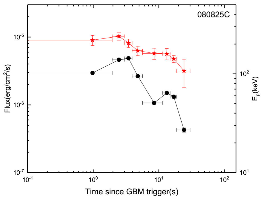
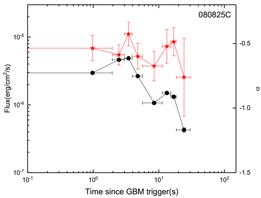
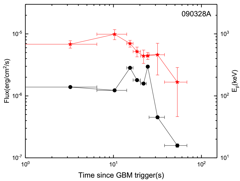
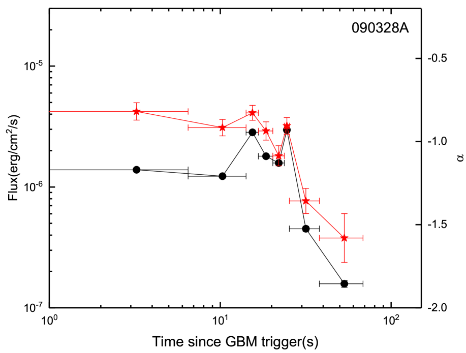
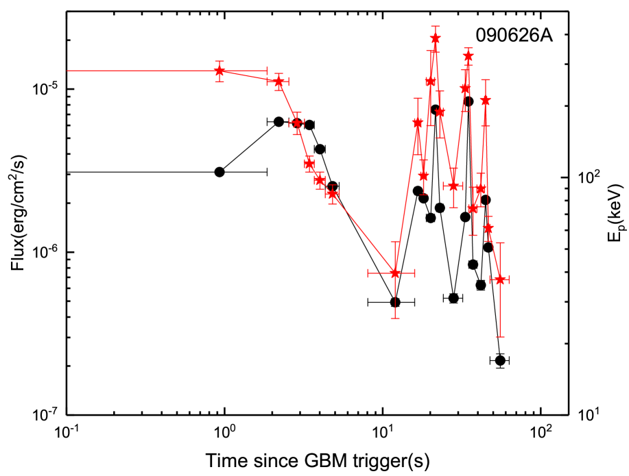
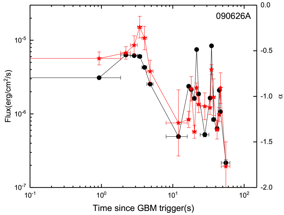
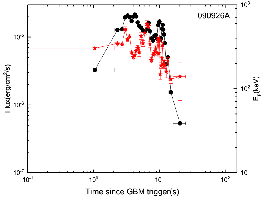
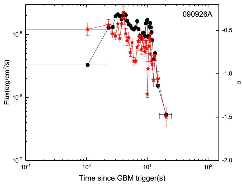
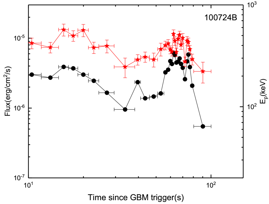
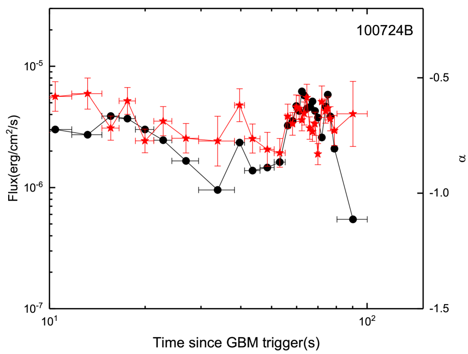
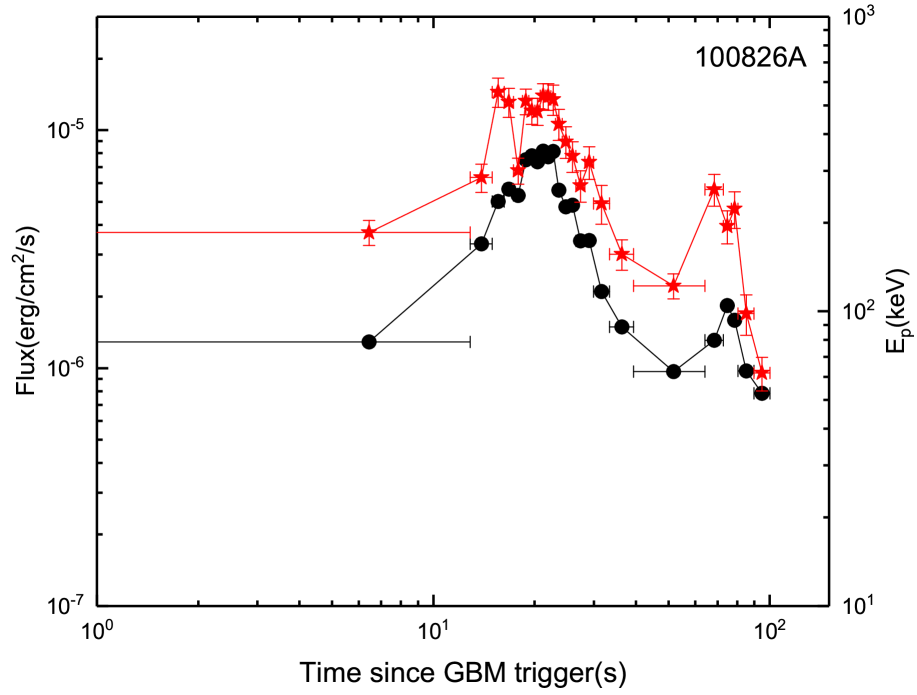
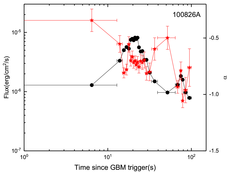
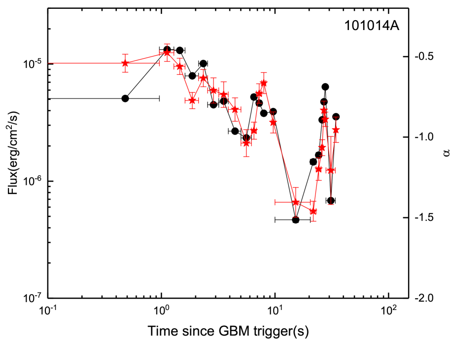
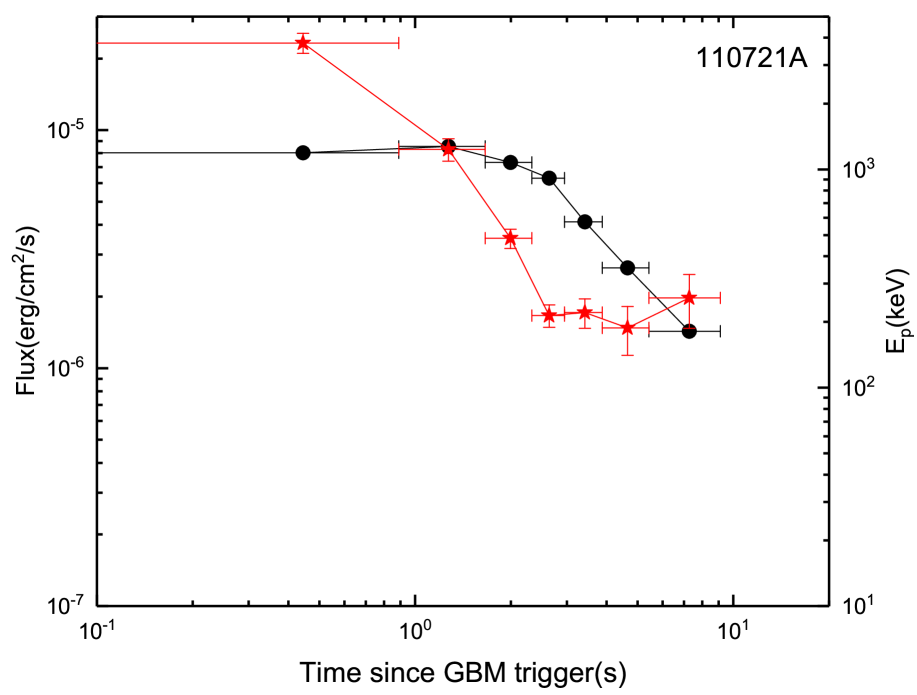
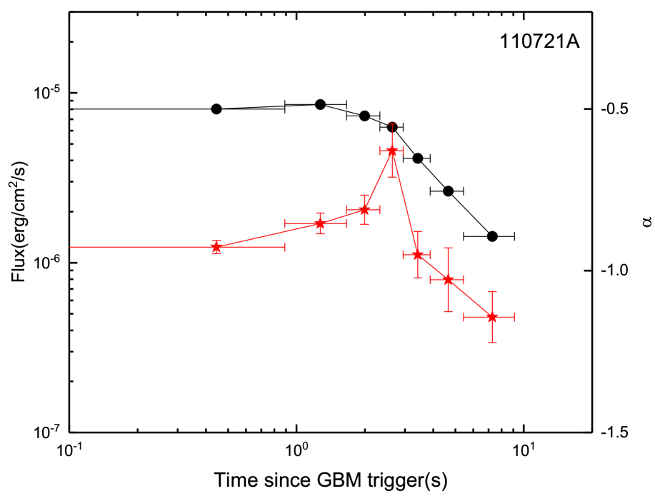
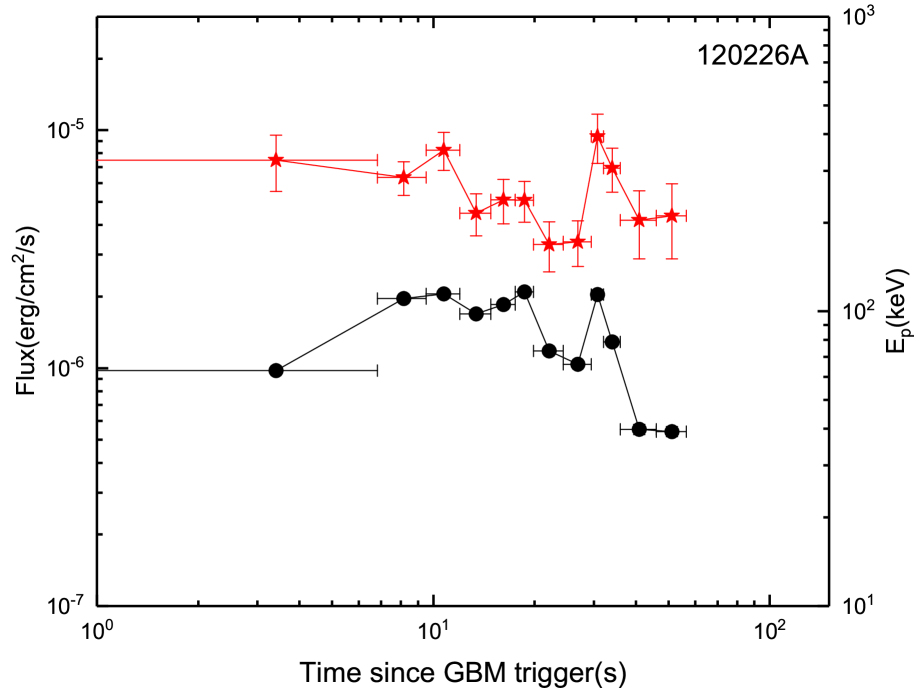
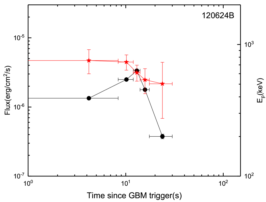
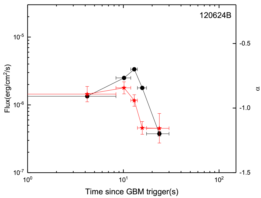
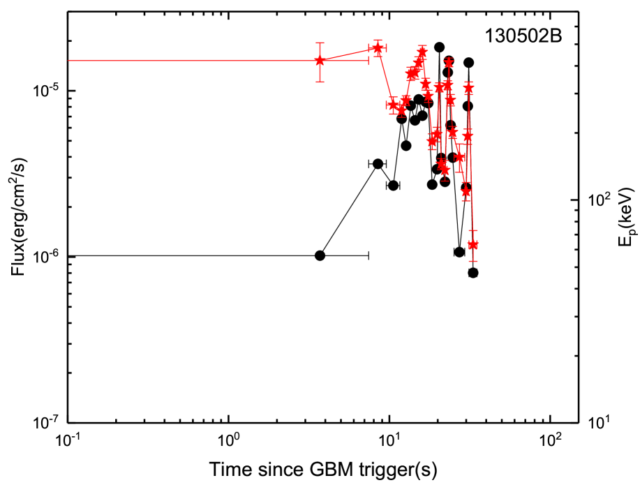
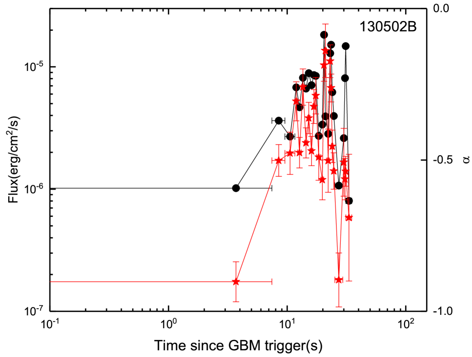
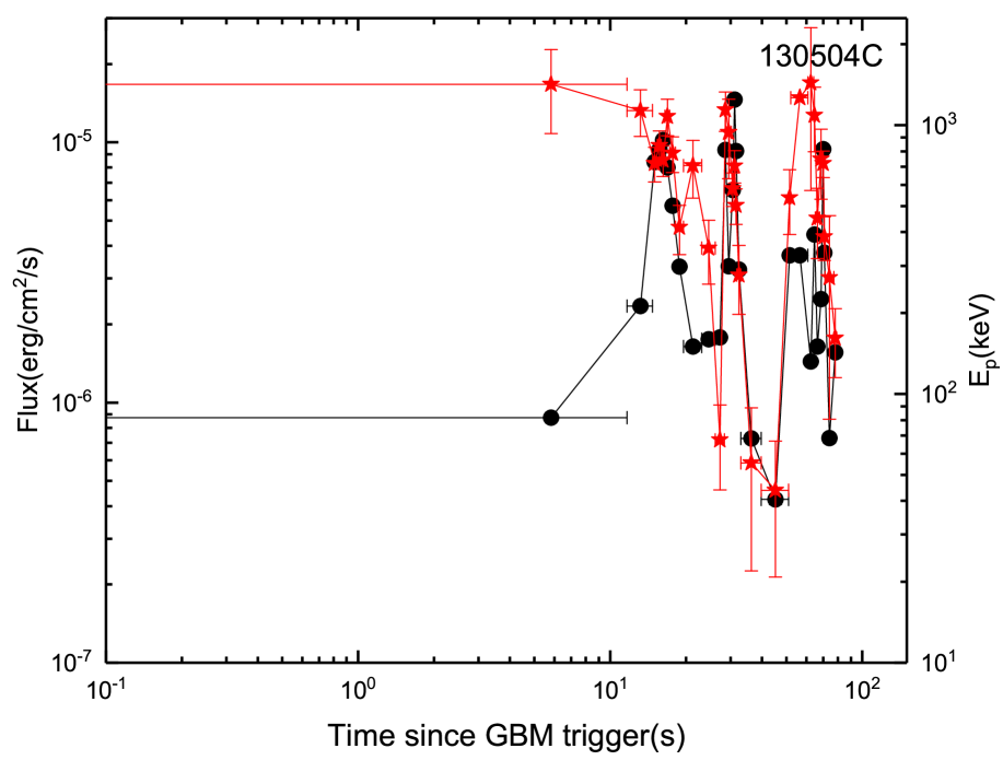
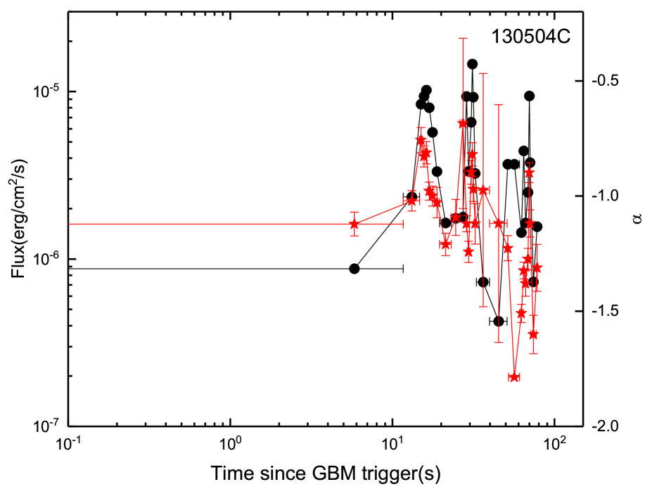
Figure 6: Spectral evolutions. The temporal characteristics of energy flux for all bursts in our sample (the left-hand, y-axis), along with time evolutions of $E_{p}$ and $\alpha$, both are marked with red stars in the right-hand y-axis.

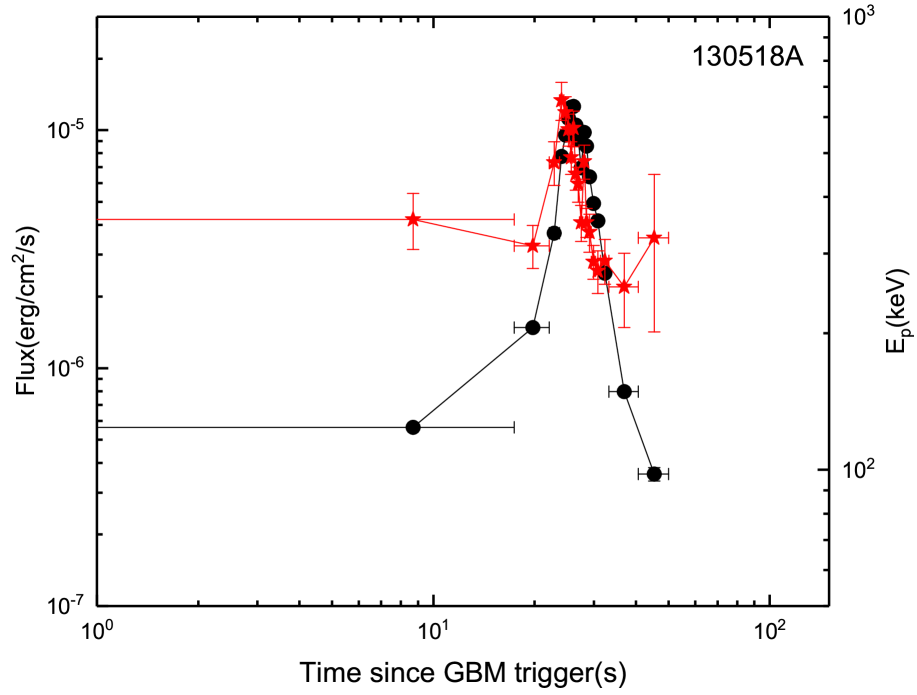
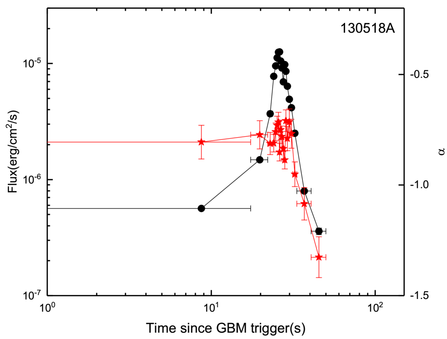
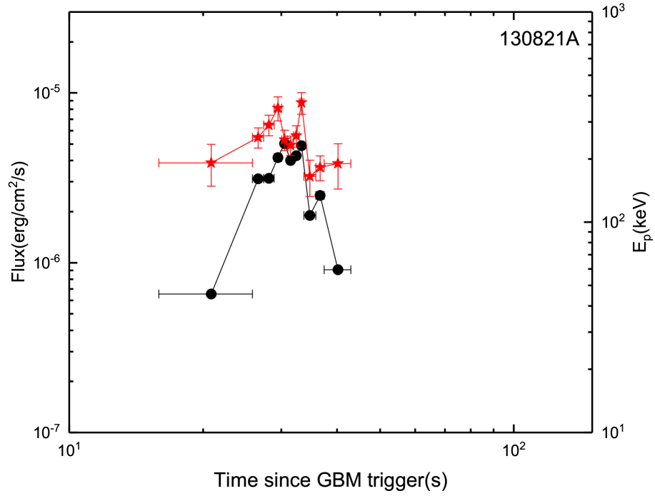
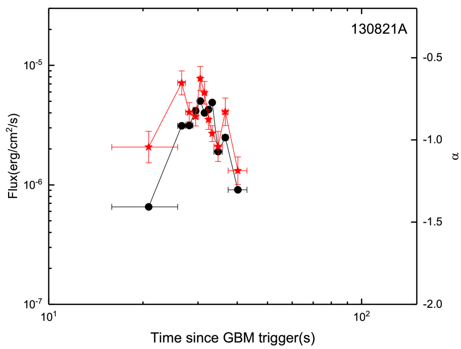
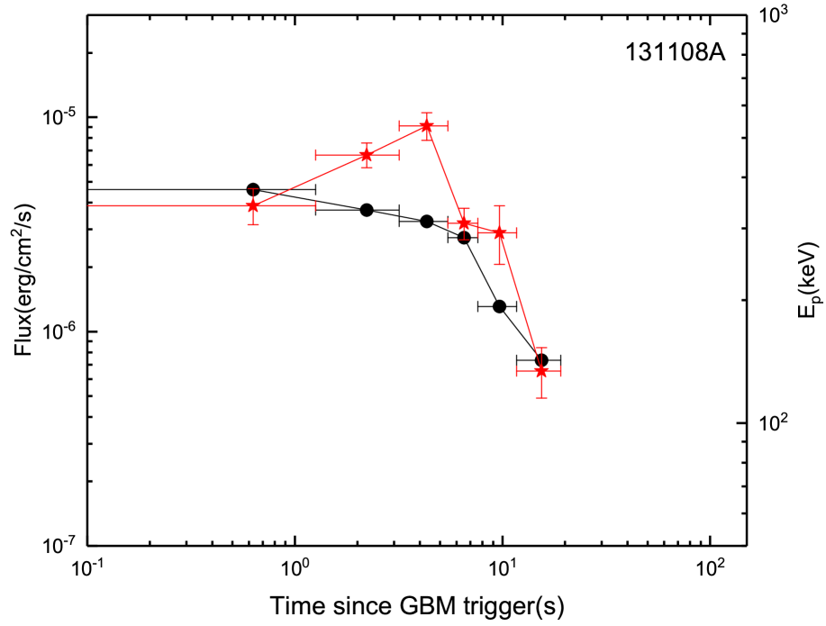
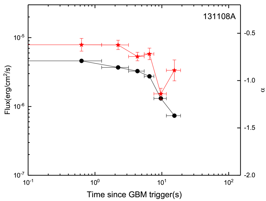
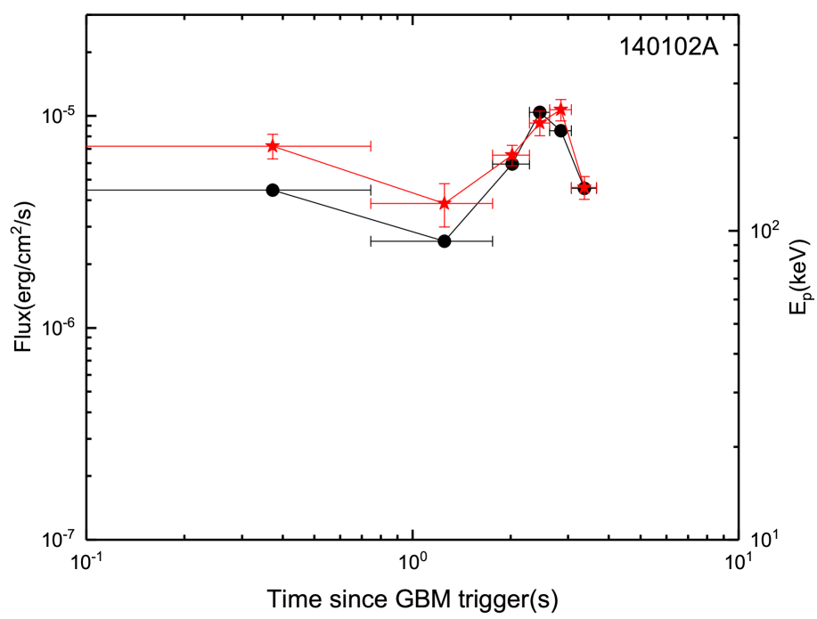
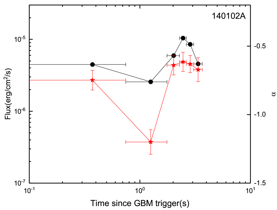
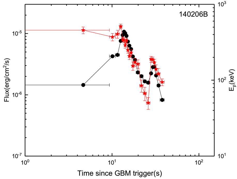
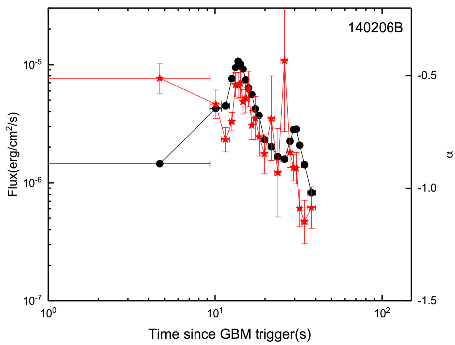
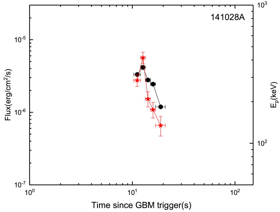
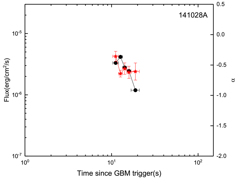
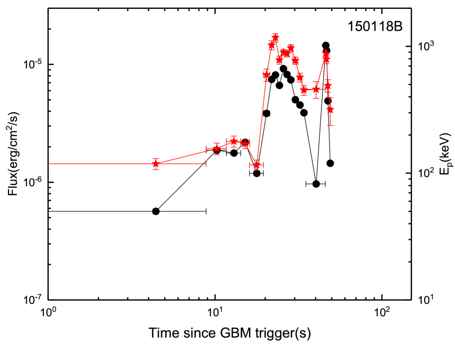
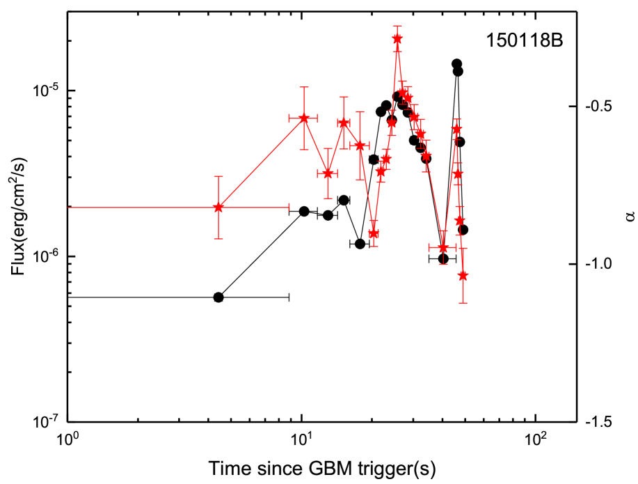
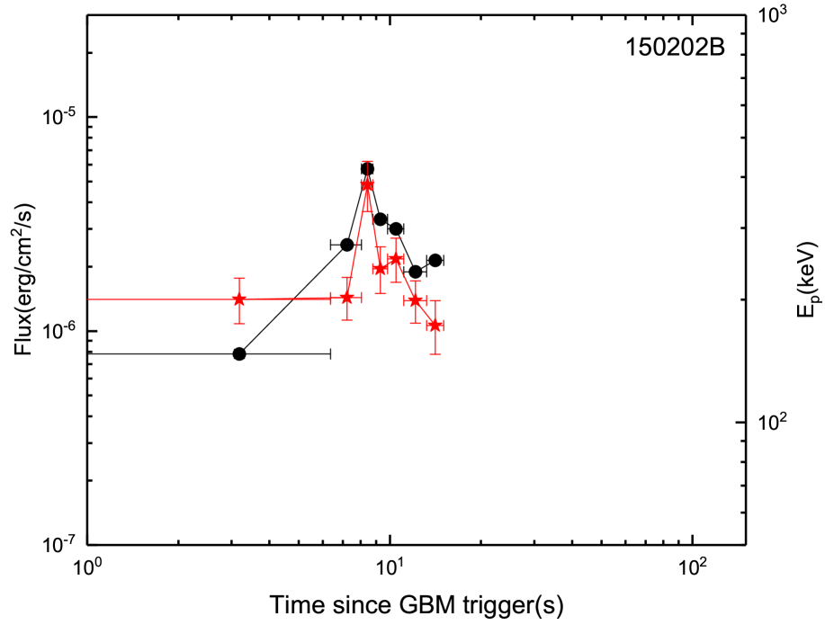
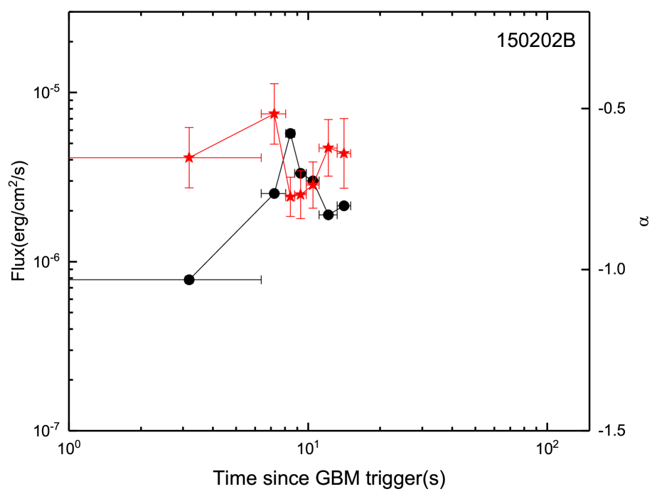
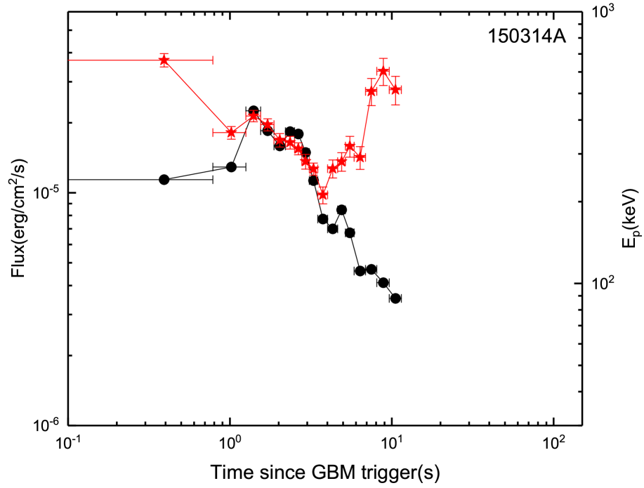
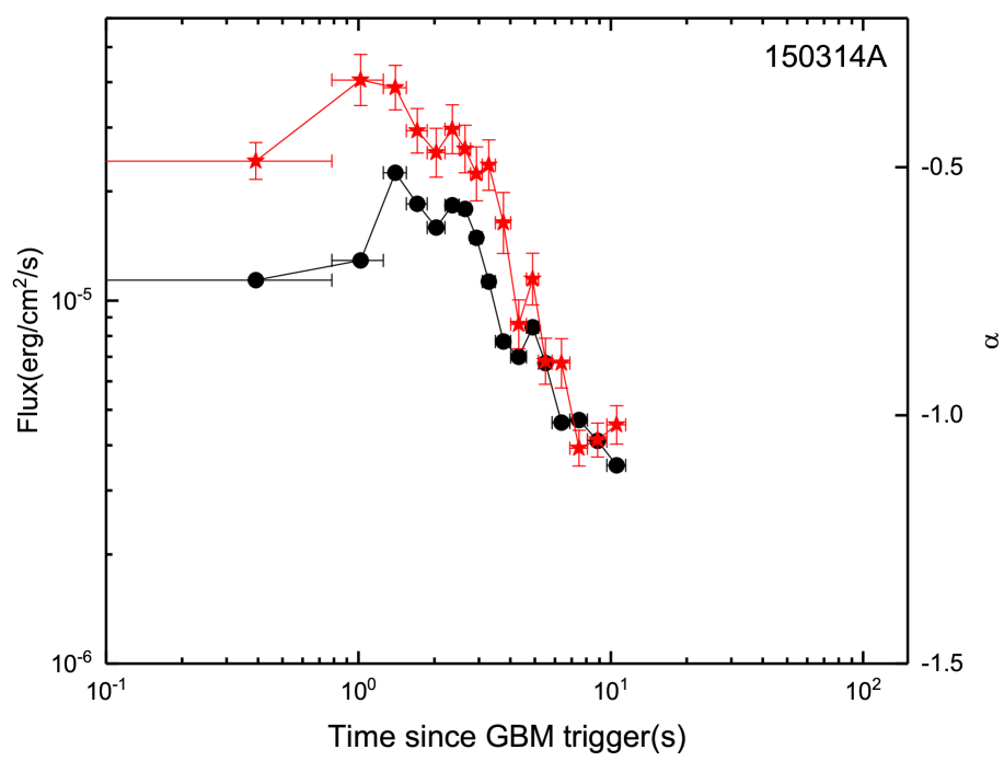
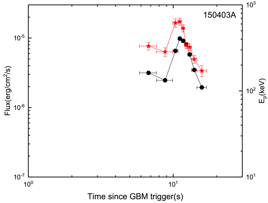
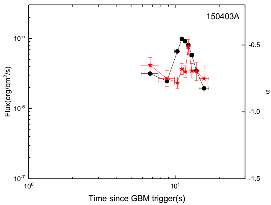
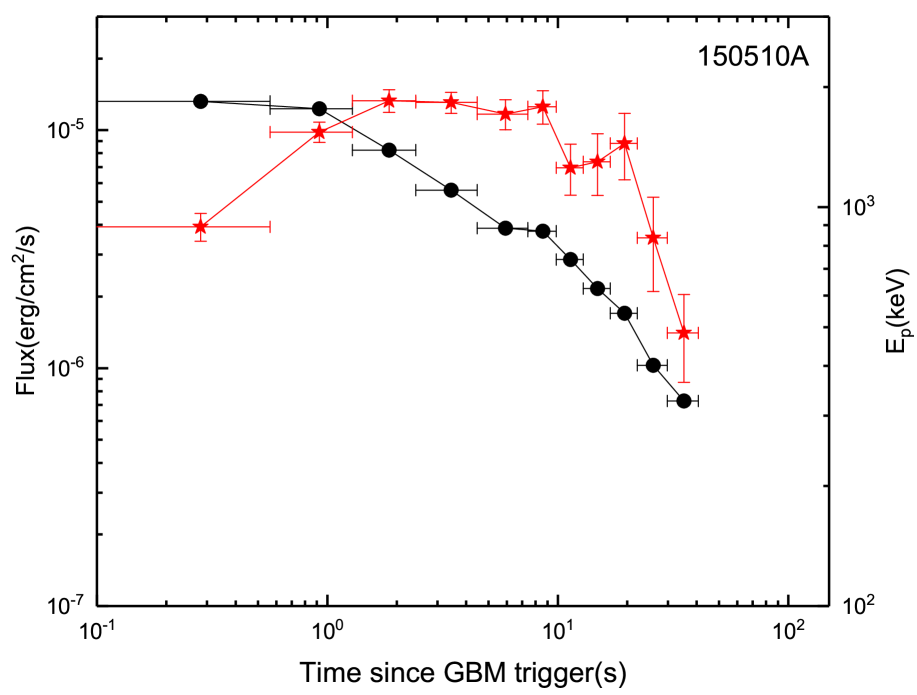
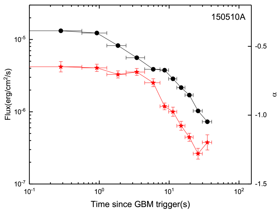
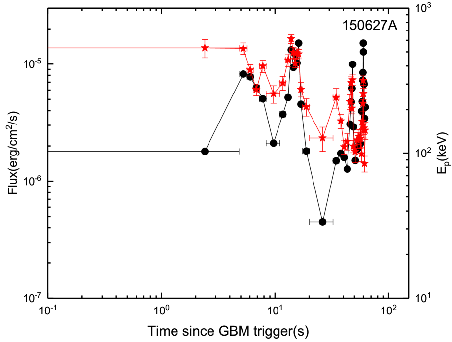
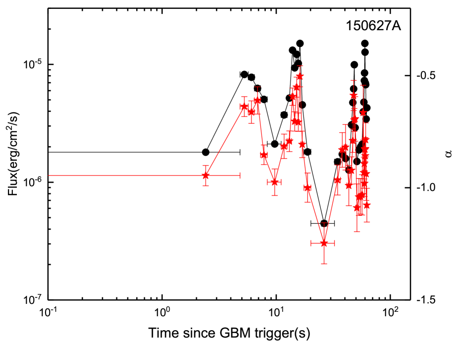
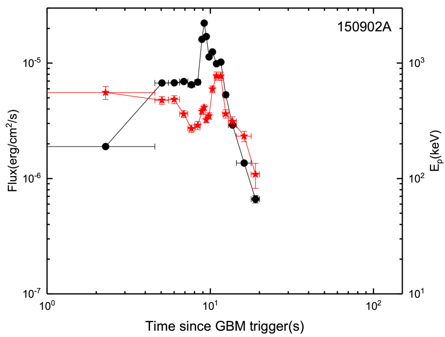
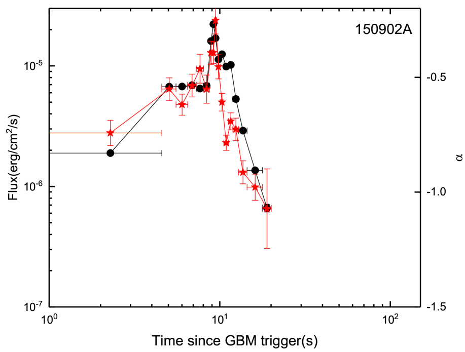
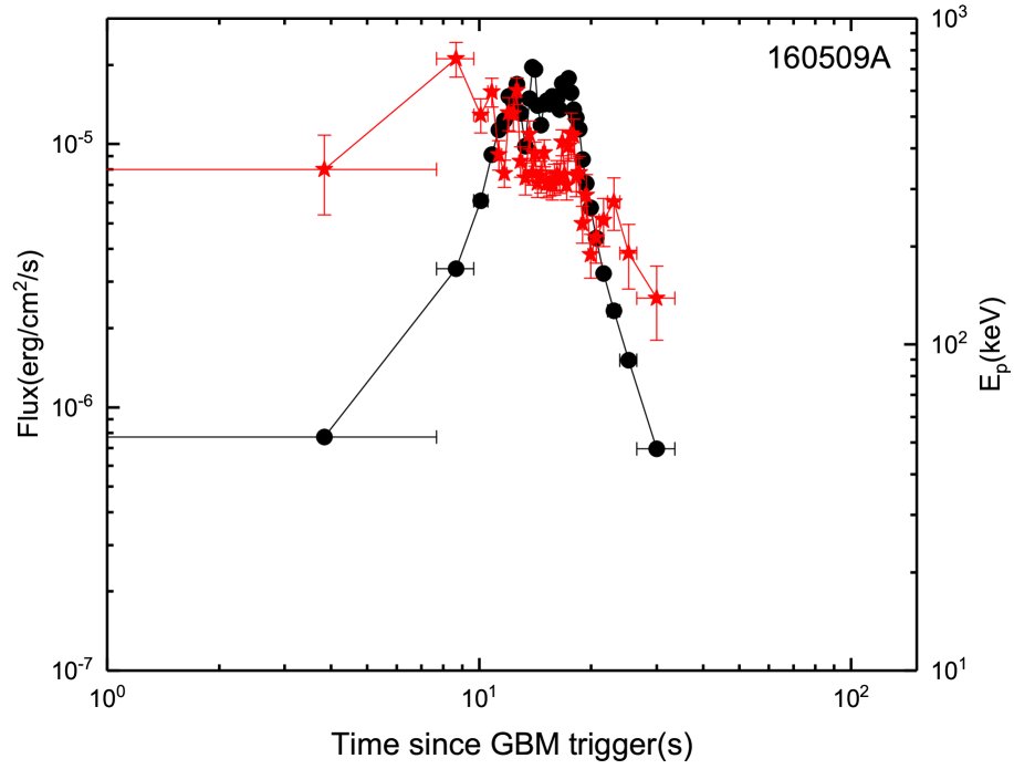
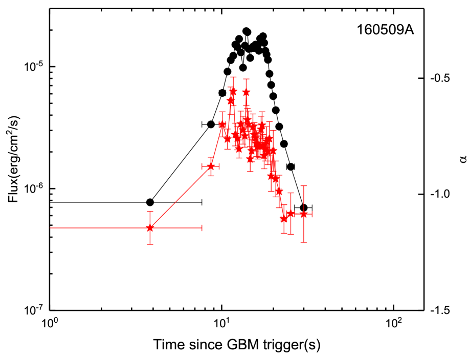
Figure 6: -continued

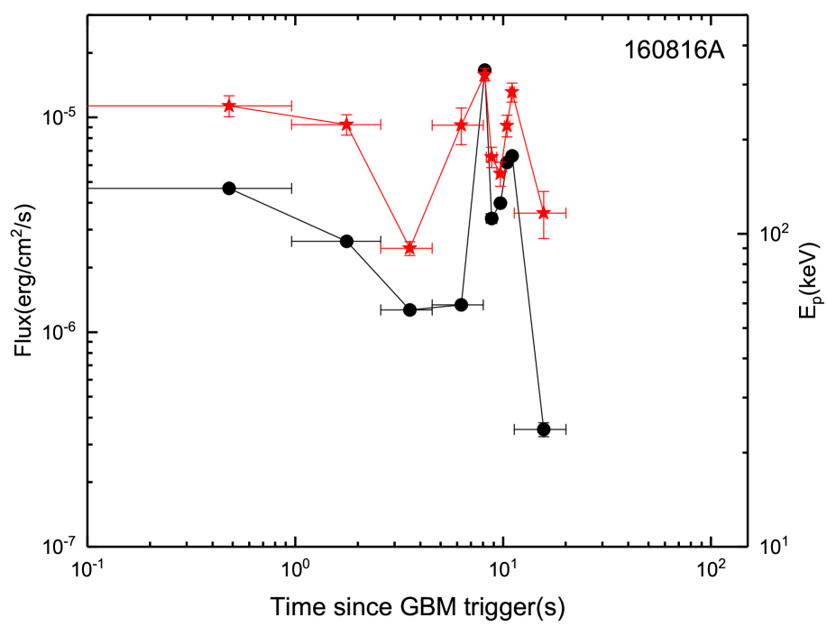
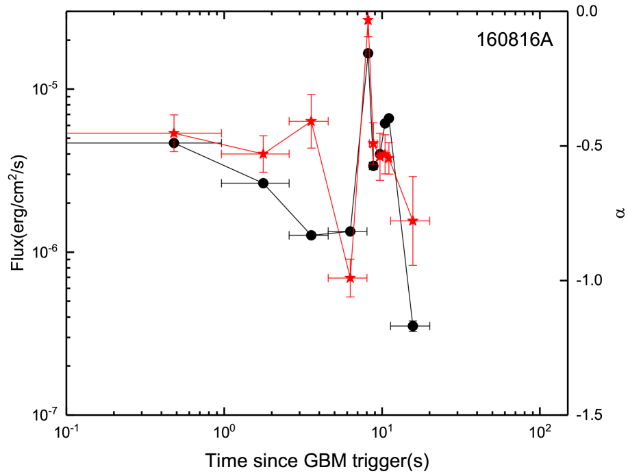
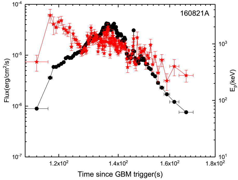
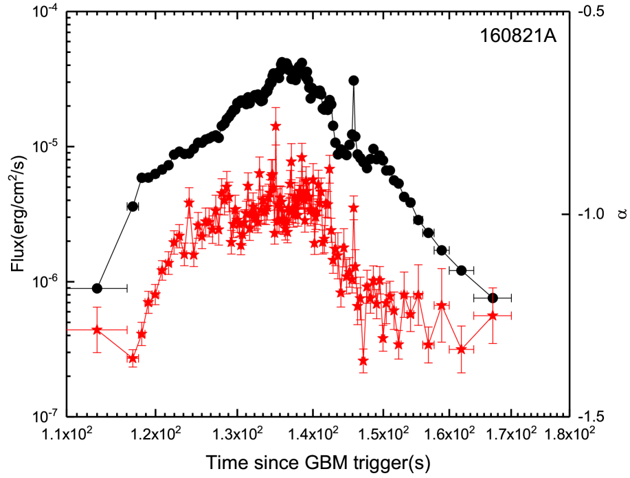
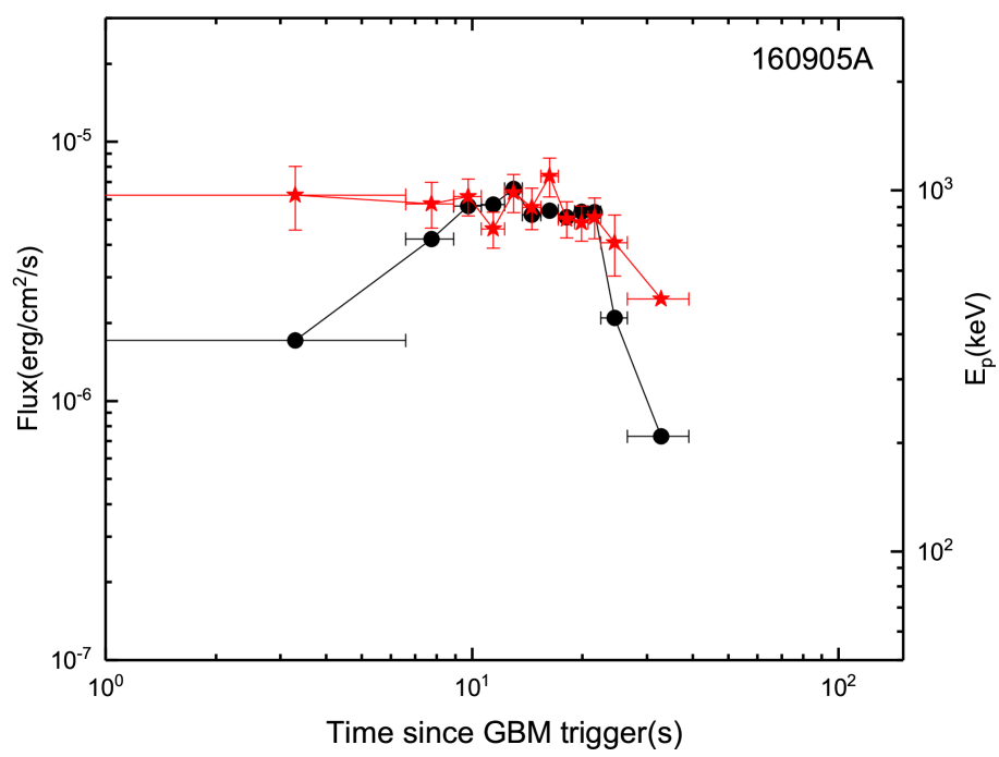
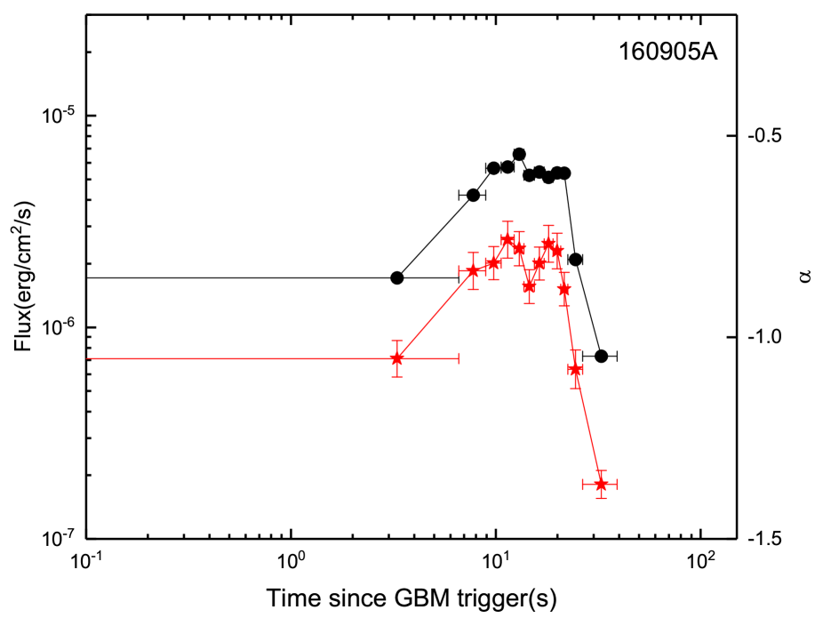
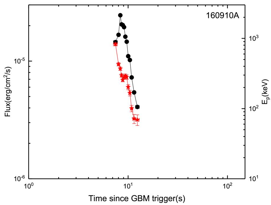
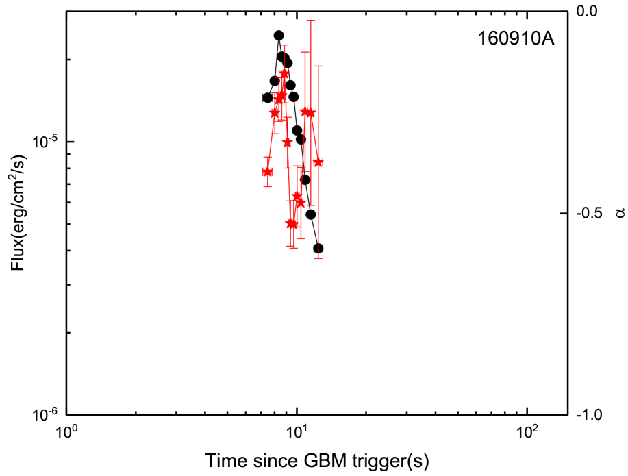
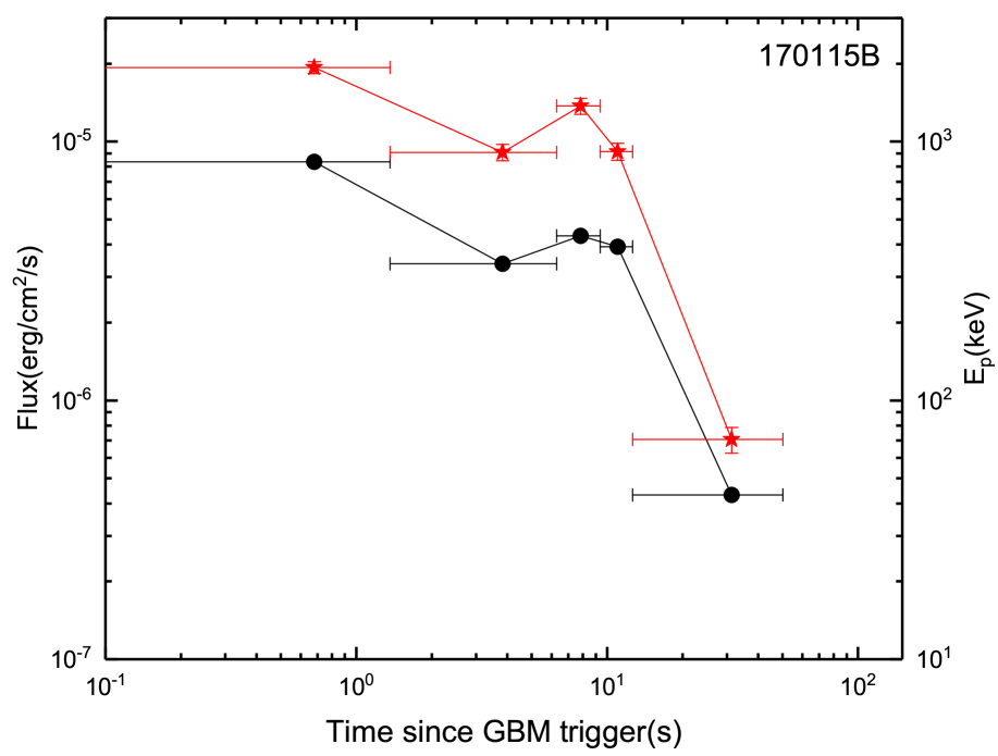
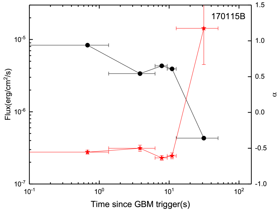
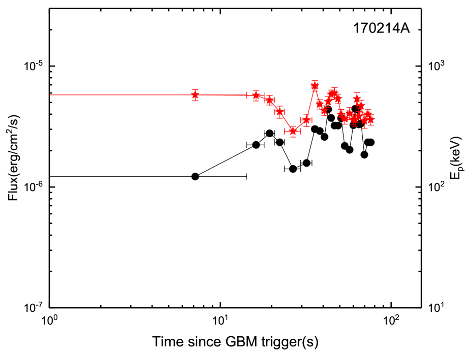
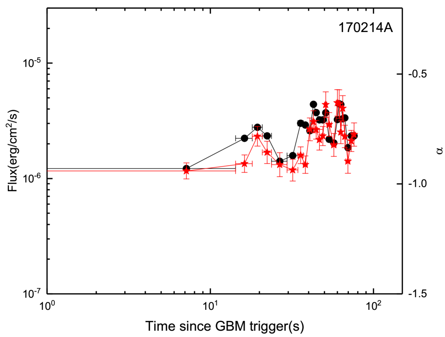
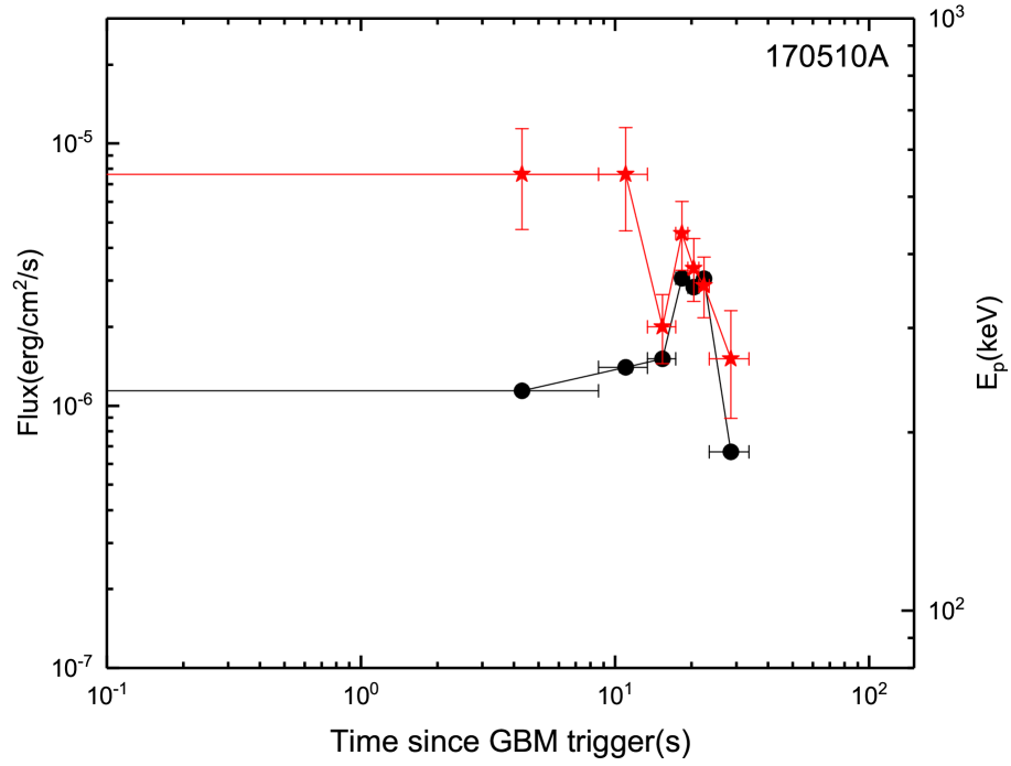
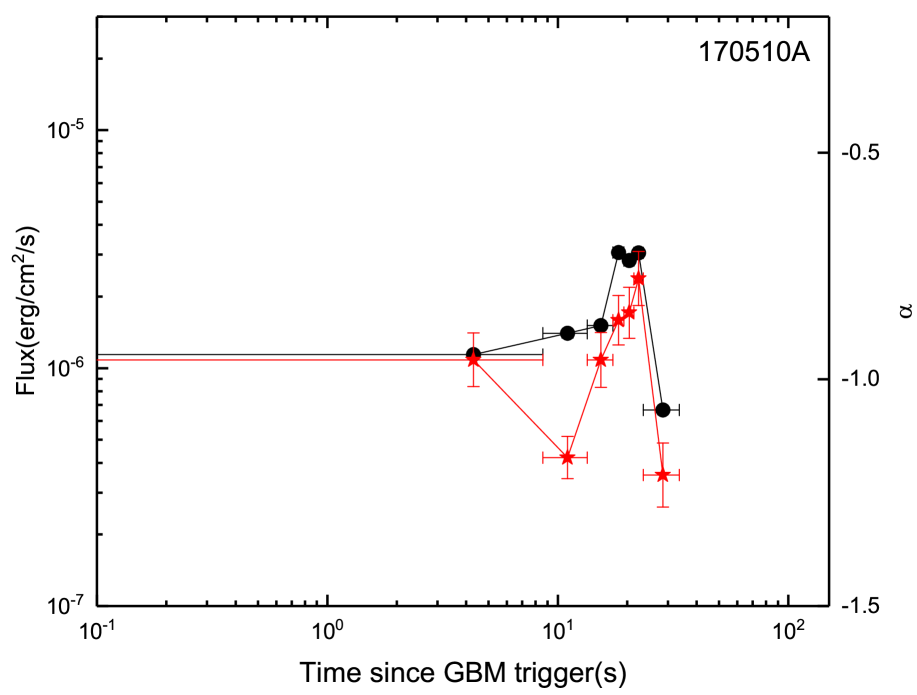
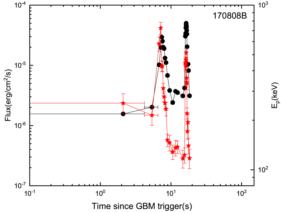
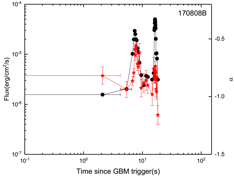
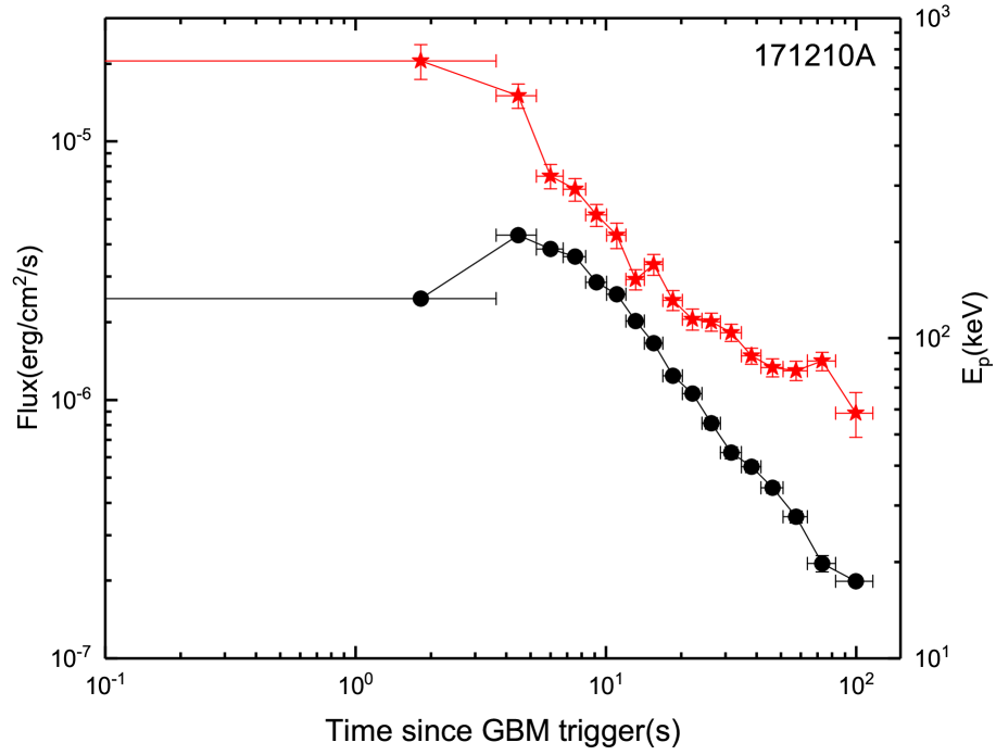
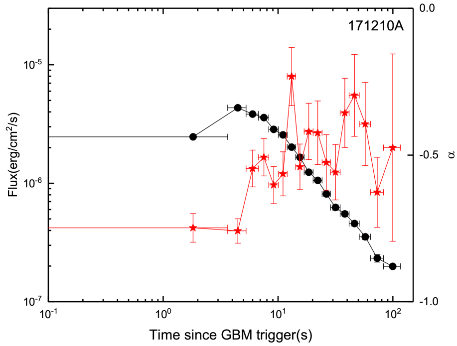
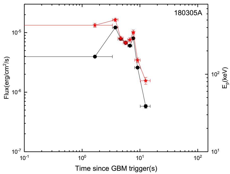
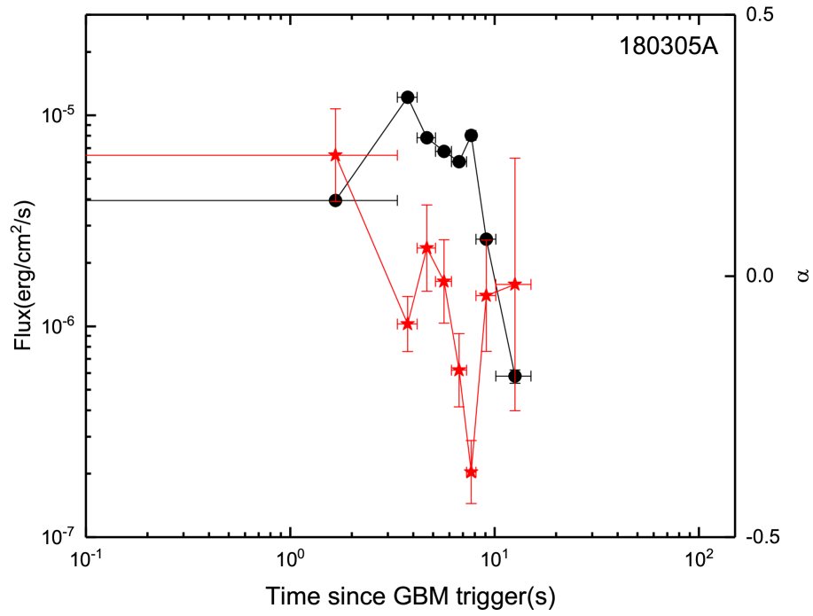
Figure 6: -continued

Figure 7: The histograms of $E_{p}$ and $\alpha$ in detailed time-resolved spectra. The left panel is the histogram of $E_{p}$, the typical value of $E_{p}$ is from 200 to 400 keV. The right panel shows the histogram of $\alpha$, the typical value is $\sim-0.8$. The typical value is consistent with the statistical study of large sample in previous literatures both for $E_{p}$ and $\alpha$ in all spectra.

We present the results of time-resolved spectral analysis and the evolution patterns of $E_{p}$ and $\alpha$ . The fitting results of the parameter correlations and the spectral evolutions of $E_{p}$ and $\alpha$ have been shown in Table 3. Listed in this Table are the GRBs in our sample which satisfy our criteria in this study (Col.1), the detectors used (Col.2), the number of the time slice (Col.3), the Pearson’s correlation coefficient r in the $E_{p}-F$ correlation (Col.4), the Pearson’s correlation coefficient r in the $\alpha-F$ correlation (Col.5), the Pearson’s correlation coefficient r in the $E_{p}-\alpha$ correlation (Col.6), the spectral evolution patterns of $E_{p}$ and $\alpha$ (Col.7), whether the values of $\alpha$ in time-resolved spectral analysis are larger than the synchrotron limit ($-\frac{2}{3}$) or not (Col.8), Figure 6 shows the spectral evolutions for The histograms of $E_{p}$ and $\alpha$ obtained by performing the detailed time-resolved spectral analysis have been shown in Figure 7.

As described above, there are three types for the evolution patterns of peak energy $E_{p}$: (i) ‘hard-to-soft’ trend; (ii) ‘flux-tracking’ trend; (iii) ‘soft-to-hard’ trend or chaotic evolutions. recent study pointed out that the first two patterns are dominated. A good fraction of GRBs follow ‘hard-to-soft’ trend (about two-thirds), the rest should be the ‘flux-tracking’ pattern (about one-third). While the low energy photon index $\alpha$ does not show strong general trend compared with $E_{p}$ although it also evolves with time instead of remaining constant. All of these results can be contributed to the statistical study for the large sample of bursts in the previous literatures. give birth to different and new progress in the field of the $Fermi$-LLE bursts.

We investigate Figure 6 in detail and . In fact, the evolution pattern of $E_{p}$, GRBs exhibit the ‘hard-to-soft’ pattern; 2 GRBs undergo the transition from ‘soft-to-hard’ to ‘hard-to-soft’ (GRBs 131108A and 150510A); GRBs show the ‘intensity-tracking’ (compared with flux); GRBs, a good fraction of those samples exhibit the ‘rough-tracking’ (compared with flux) behavior. is obvious that the ‘flux-tracking’ pattern is very popular for most of the bursts, the total number include ‘intensity-tracking’ and ‘rough-tracking’ is , which means that percent of these bursts follow the ‘flux-tracking’ pattern. For the evolution of $\alpha$, it consists of ‘hard-to-soft’ pattern, ‘soft-to-hard’ to ‘hard-to-soft’ pattern, ‘intensity-tracking’ pattern, ‘rough-tracking’ pattern, ‘anti-tracking’ pattern, ‘rough-tracking’ combined with ‘hard-to-soft’ pattern and chaotic evolution pattern (all ‘-tracking’ patterns based on the evolution of energy flux). GRBs exhibit the ‘hard-to-soft’ pattern; 1 GRB undergoes the transition from ‘soft-to-hard’ to ‘hard-to-soft’ (GRB 110721A); 2 GRBs show ‘intensity-tracking’ pattern; most of the bursts, GRBs exhibit ‘rough-tracking’; the chaotic evolution; the rest GRBs, GRBs 150202B, 170115B, exhibit the ‘anti-tracking’ pattern shows the ‘rough-tracking’ pattern combined with ‘hard-to-soft’ pattern. All of these evolution patterns have been summarised in Table 3, one can obtain the specific evolution pattern of $E_{p}$ and $\alpha$ for each burst from table.

In addition, from Figure 7 which has presented the histograms of $E_{p}$ and $\alpha$ obtained by performing the detailed time-resolved spectral analysis, the typical value is consistent with the statistical study of large sample in previous literatures both for $E_{p}$ ($\sim$ 300 keV) and $\alpha$ ($\sim$ -0.8) in all such a value of $\alpha$ is inapplicable for some bursts such as GRBs , which the values of $\alpha$ for all slices are larger than the synchrotron limit (-$\frac{2}{3}$). Especially, GRB 170115B is different from the other three bursts because the value of $\alpha$ ($\sim-0.8$) in time-integrated spectrum is smaller than the synchrotron limit while the values in all time-resolved spectra are larger than $-\frac{2}{3}$ for the other three bursts, the value of $\alpha$ is larger than the limit both for time-integrated spectrum and each time-resolved spectrum. most of the bursts, which the ‘anti-tracking’ compared with energy flux, i.e., it is decreasing/increasing when the energy flux is increasing/decreasing. From Table 3, one can find that only GRBs can be classified as the kind that all of the values of $\alpha$ in the detailed time-resolved spectra exceed the synchrotron limit. in their detailed time-resolved spectra consist of the fraction that is larger than $-\frac{2}{3}$ and the fraction that does not exceed the synchrotron limit.

3.3 Parameter Correlations

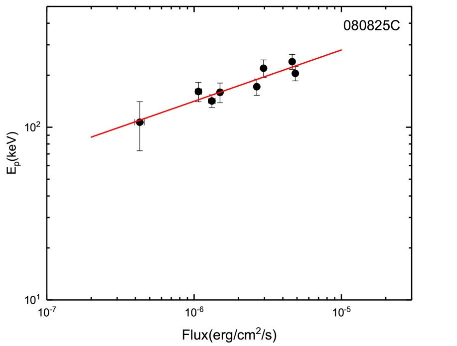
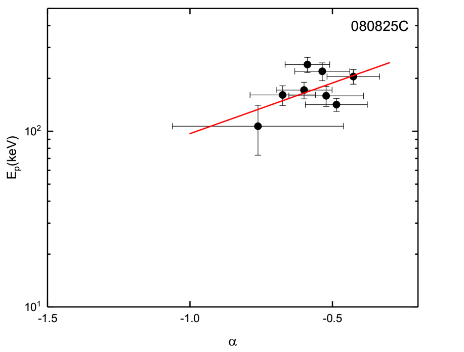
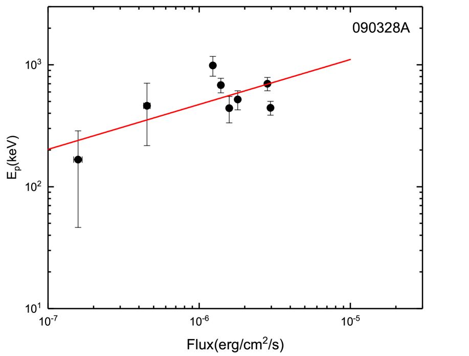
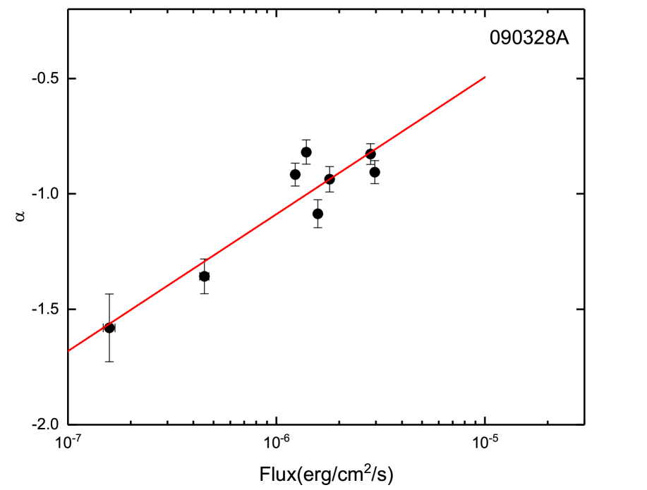
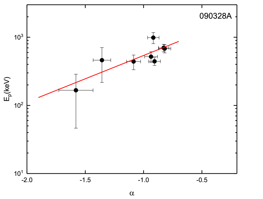
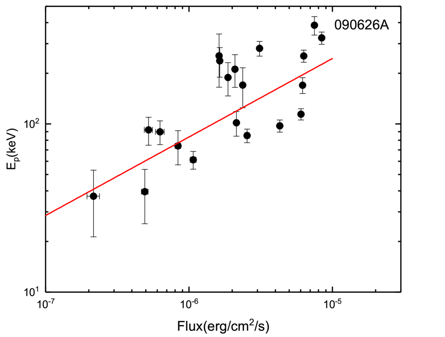
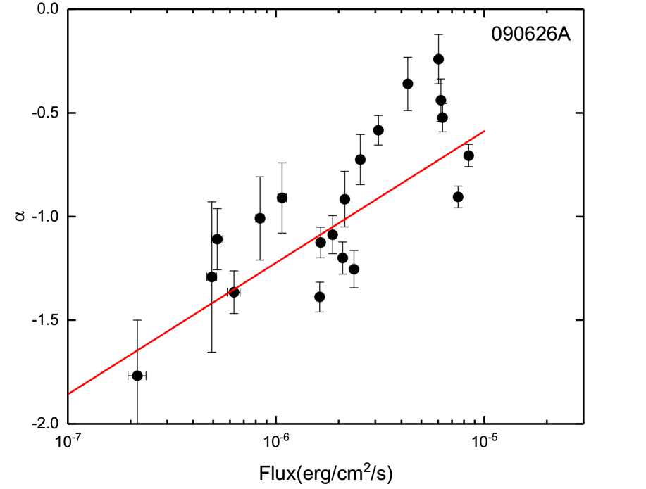
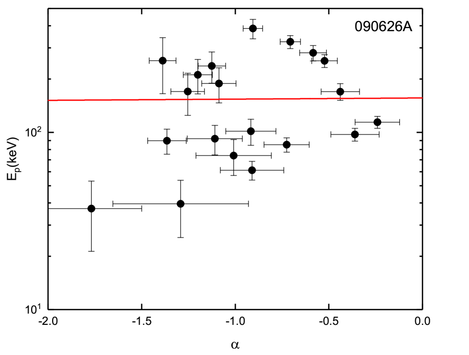
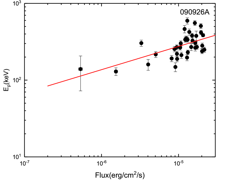
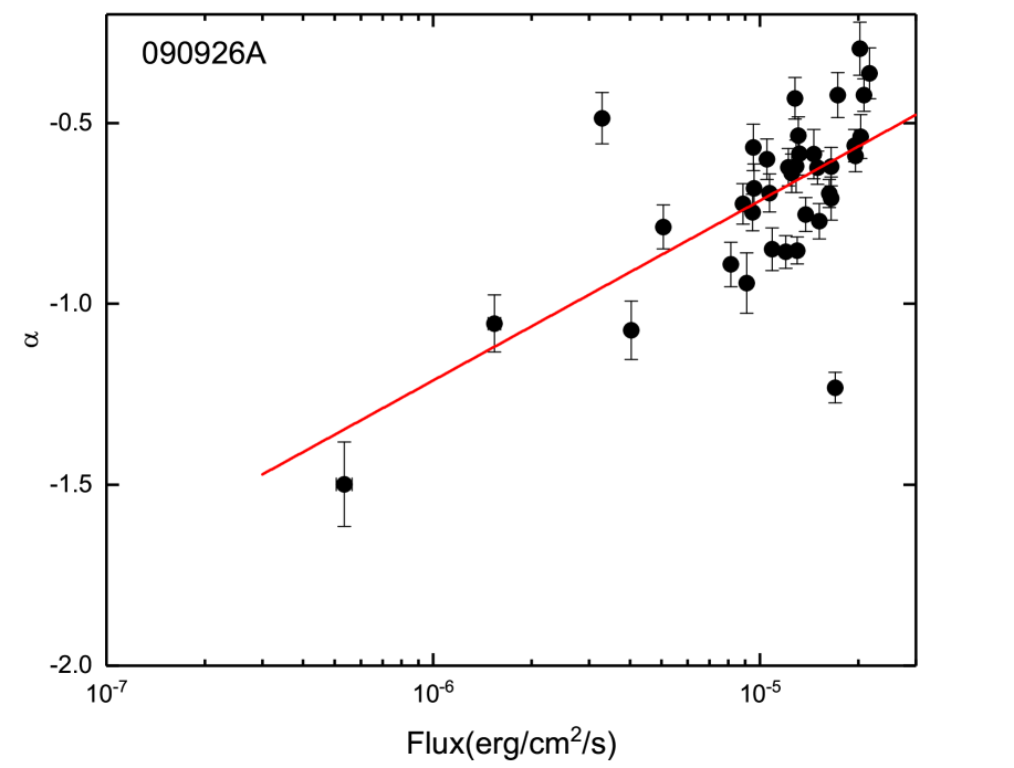
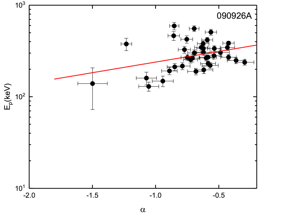
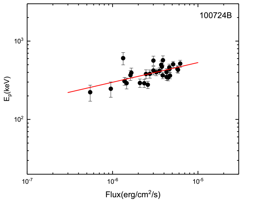
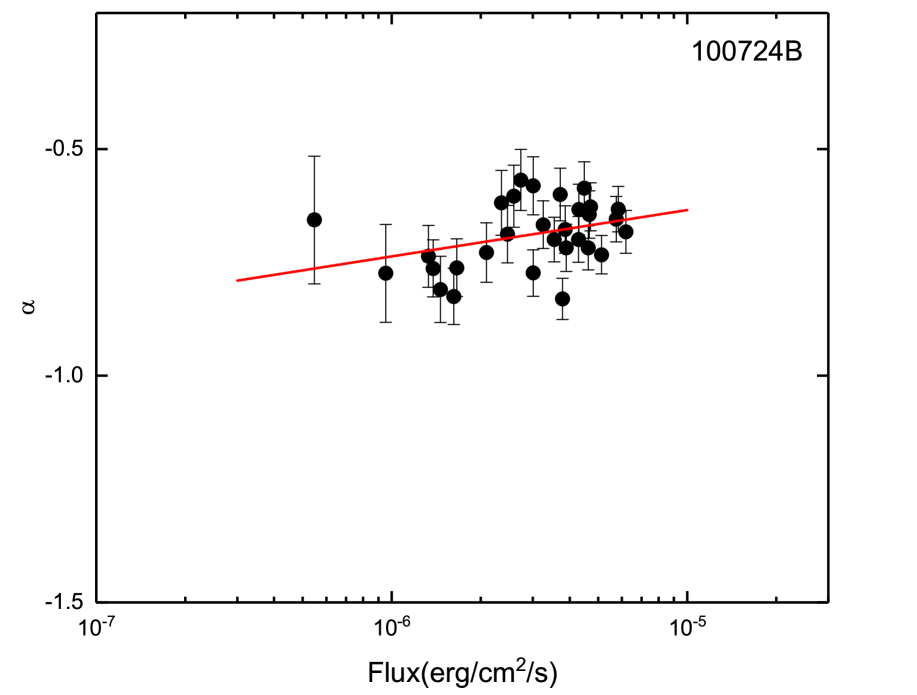
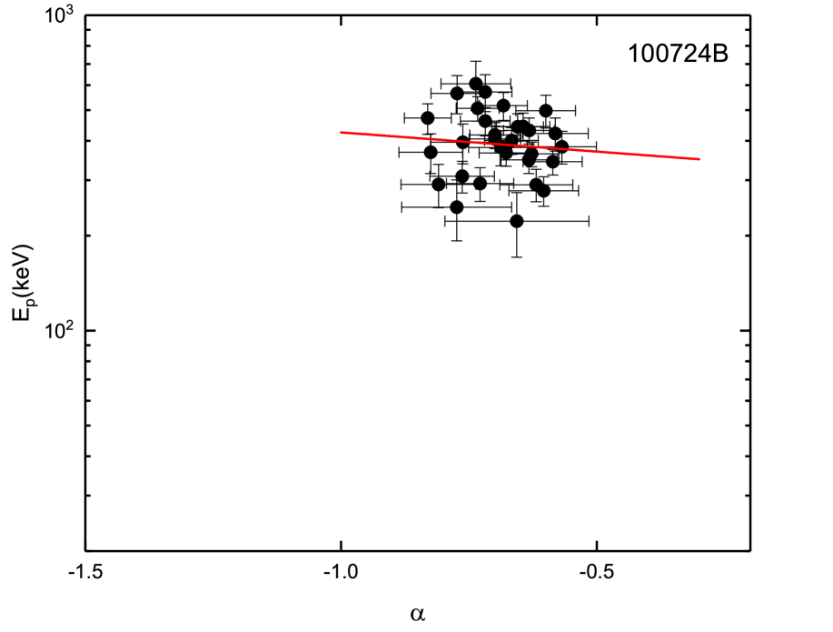
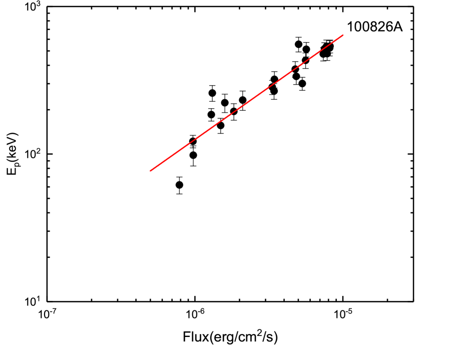
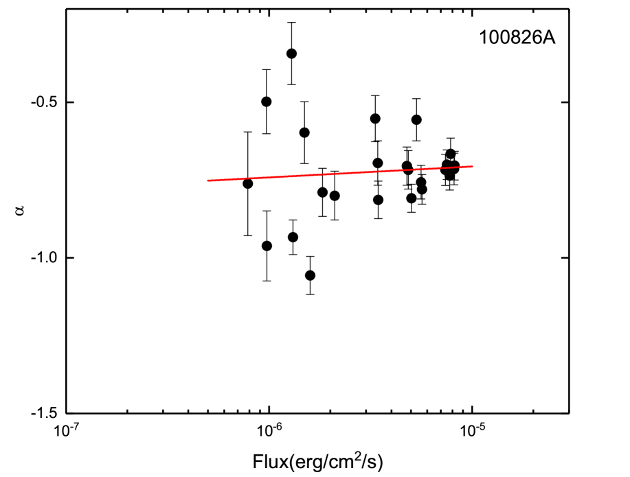
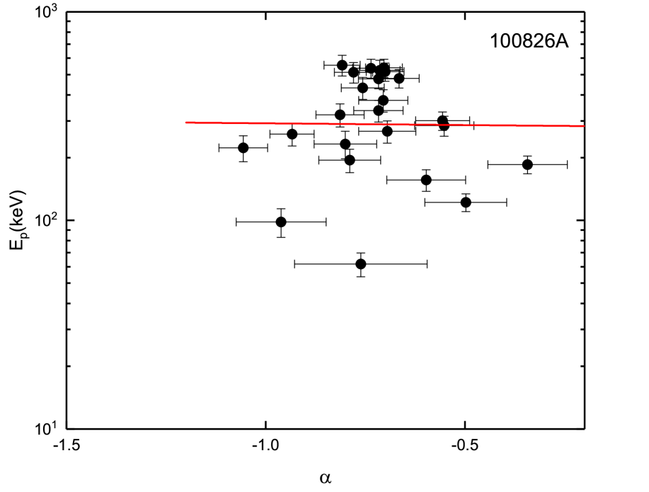
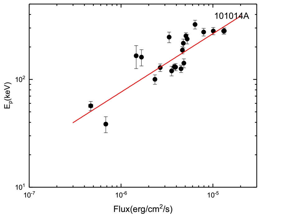
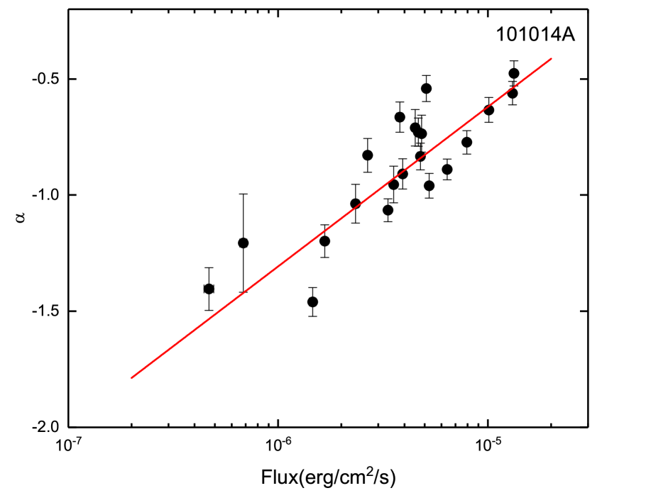
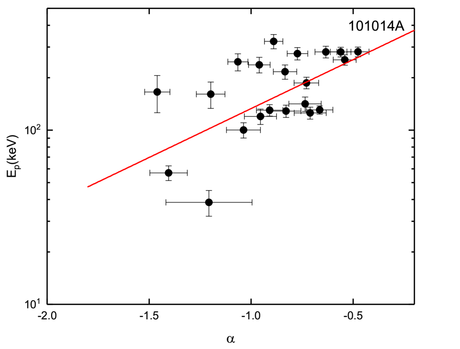
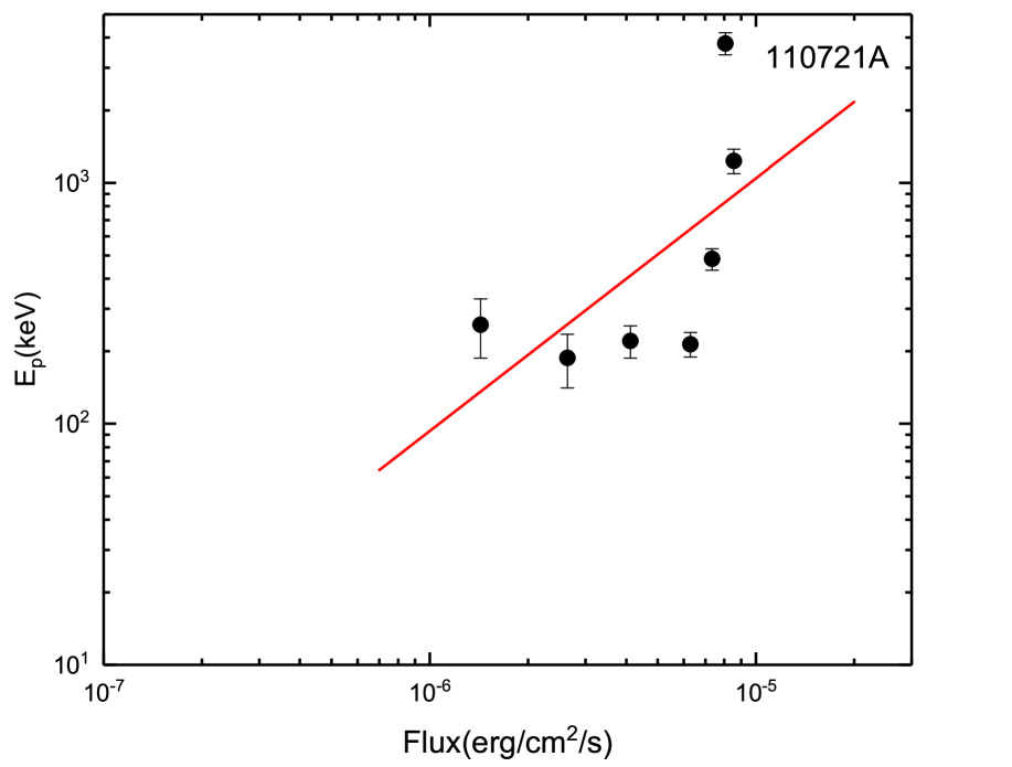
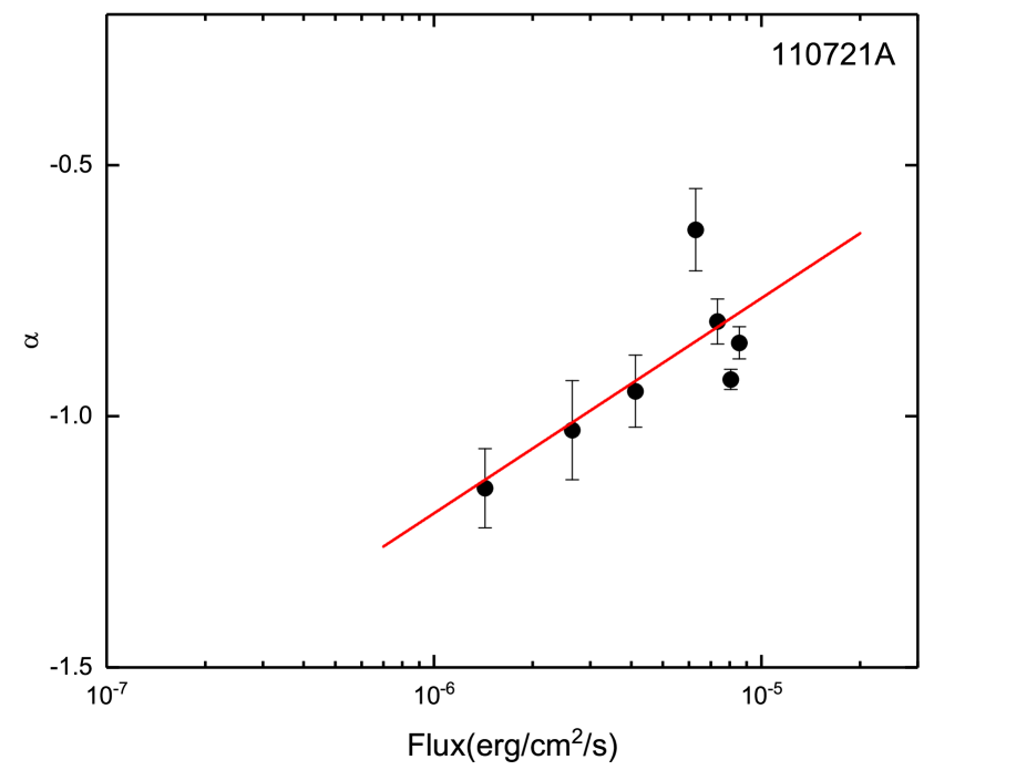
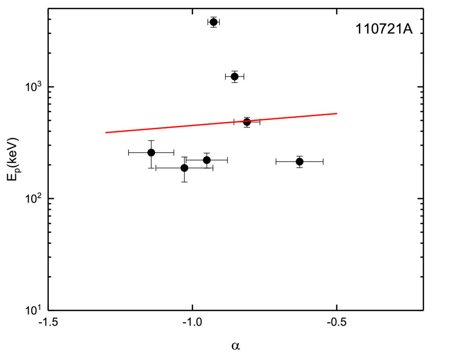
Figure 8: Parameter correlations. The correlations such as $E_{p}-F$, $\alpha-F$ and $E_{p}-\alpha$ obtained from the time-resolved spectra are shown for all of the bursts in our sample.

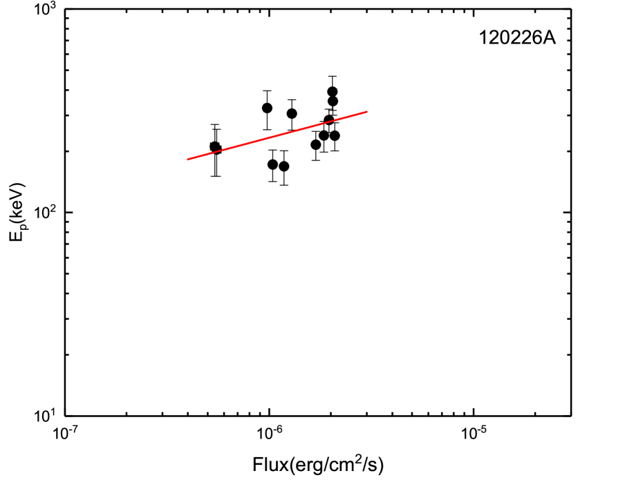
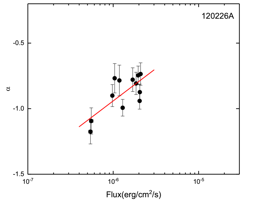
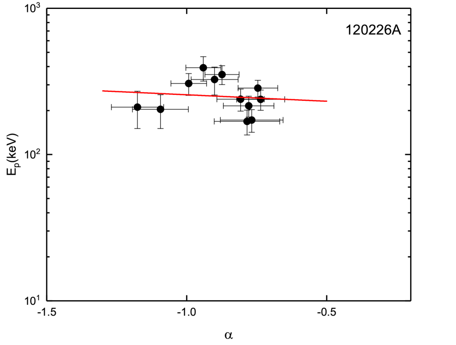
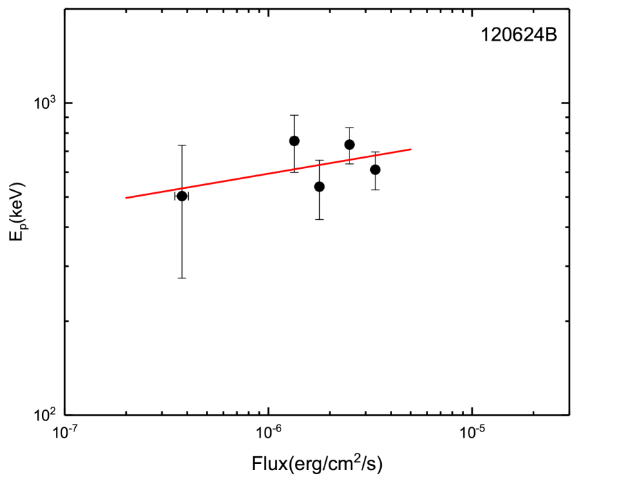
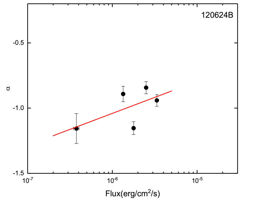
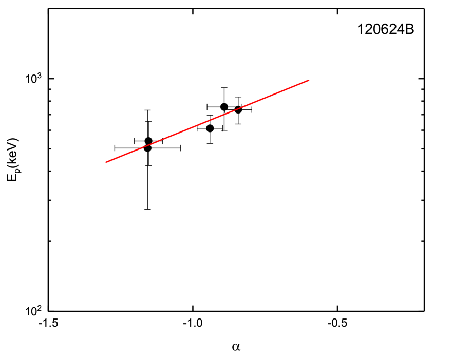
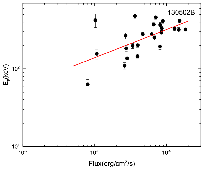
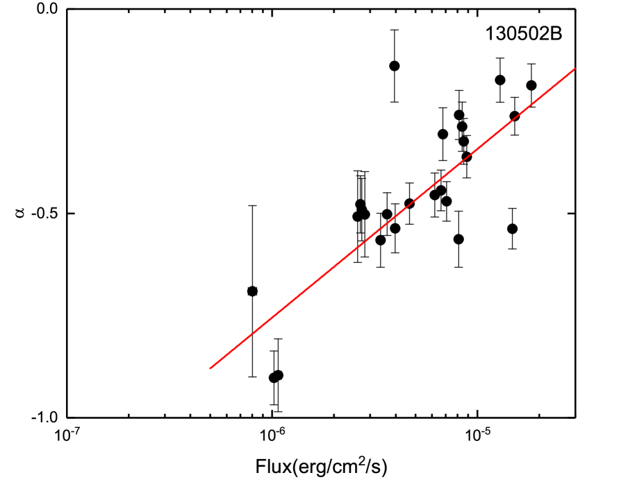
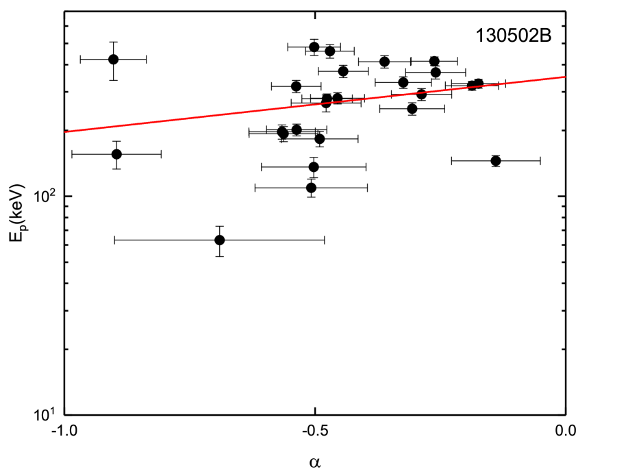
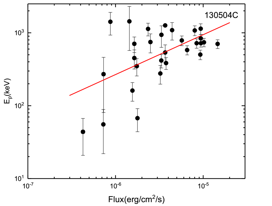
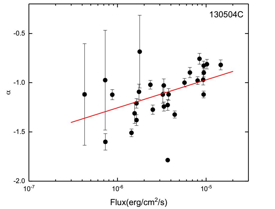
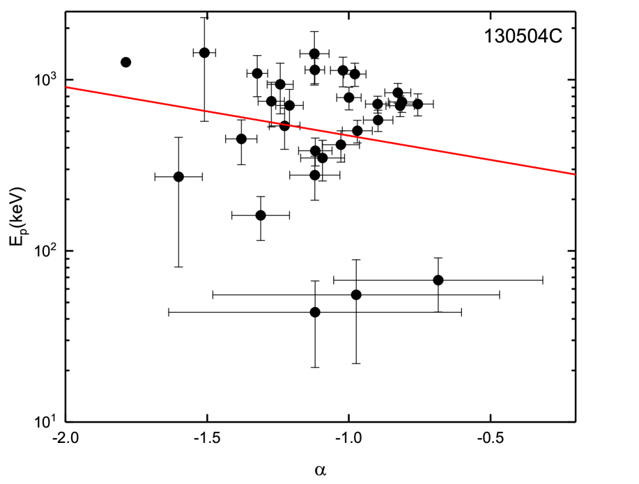
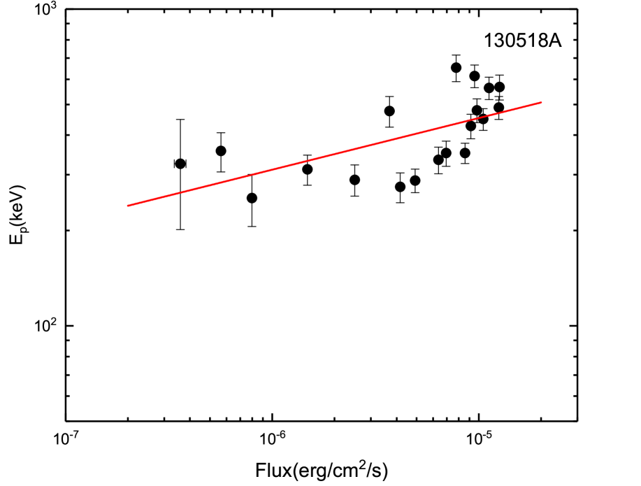
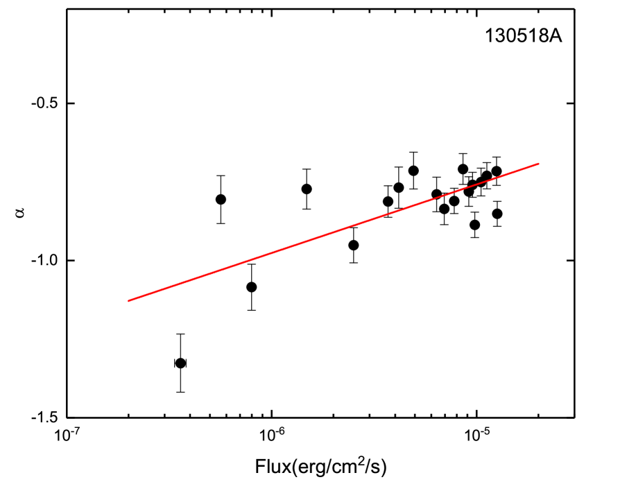
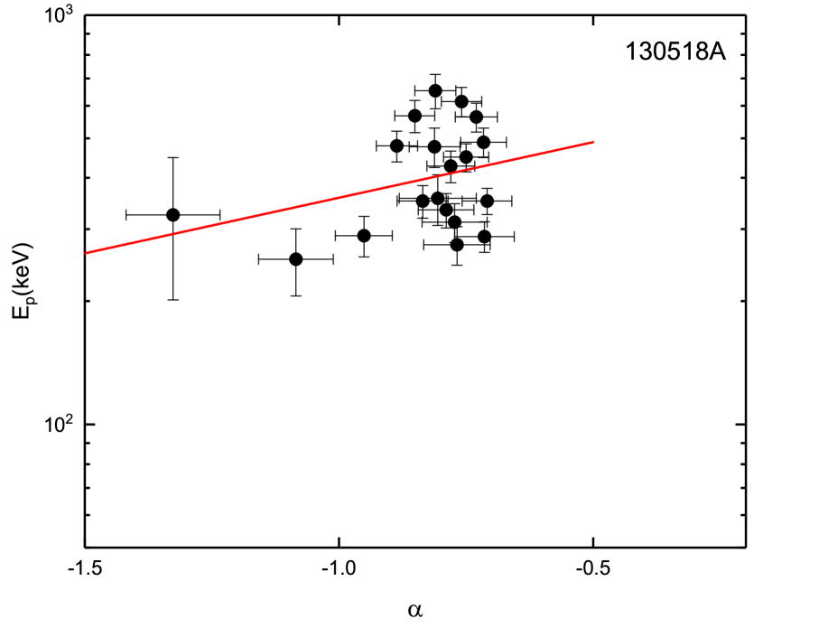
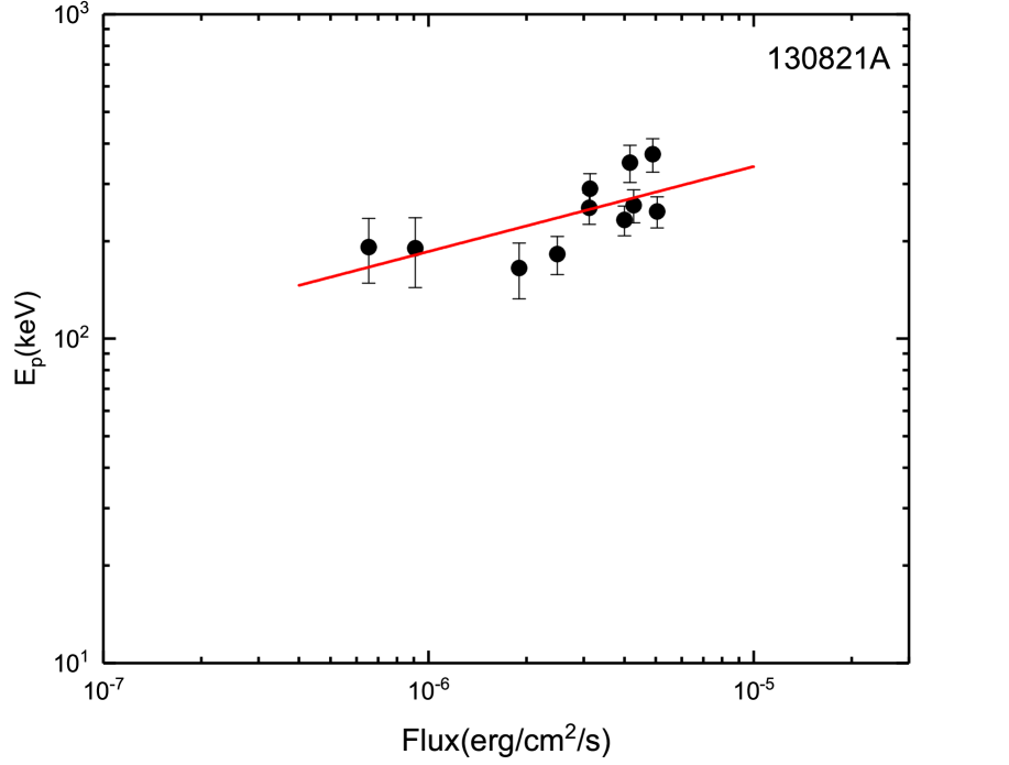
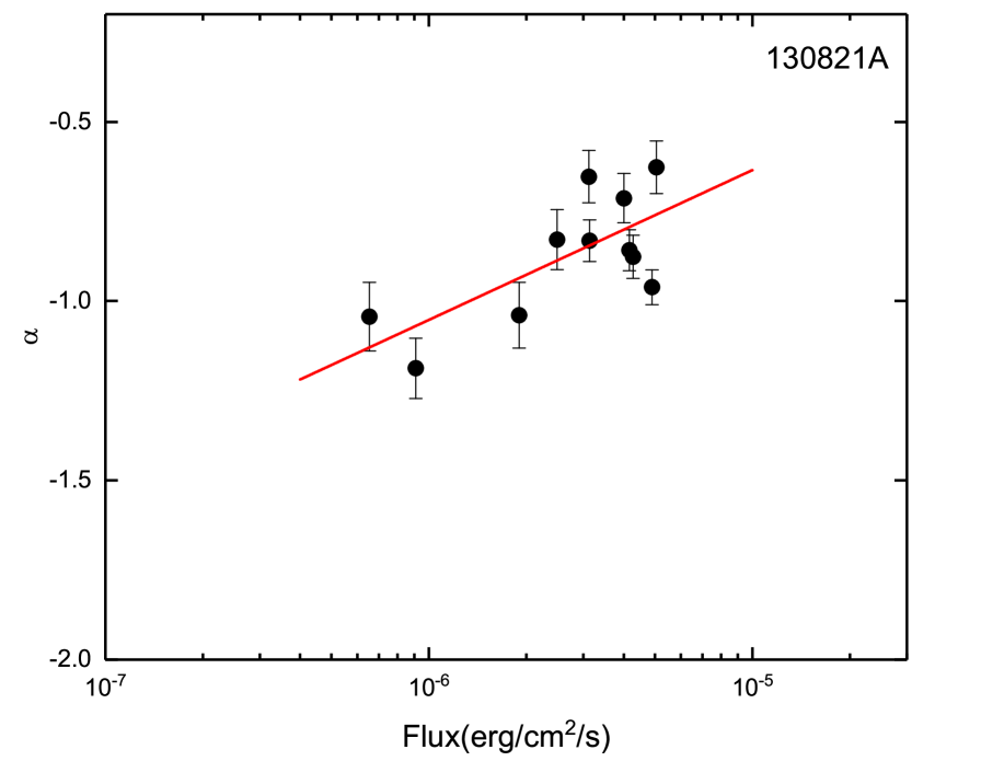
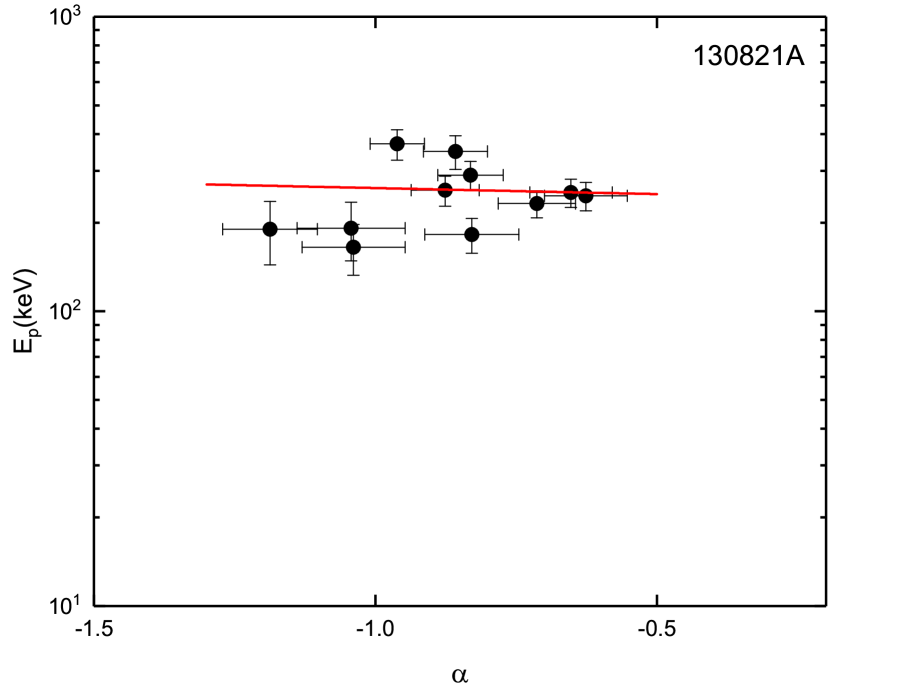
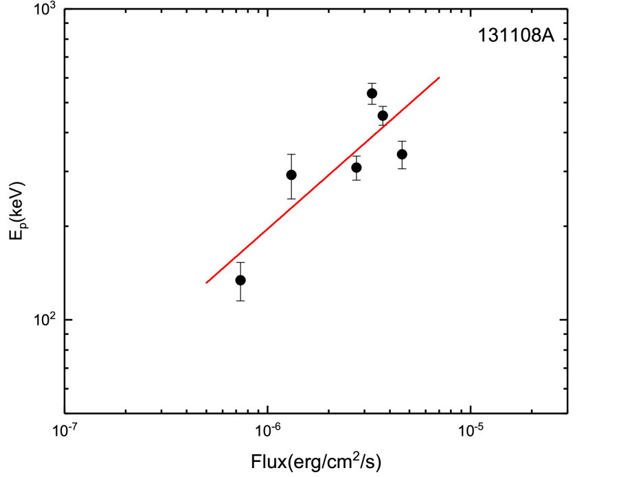
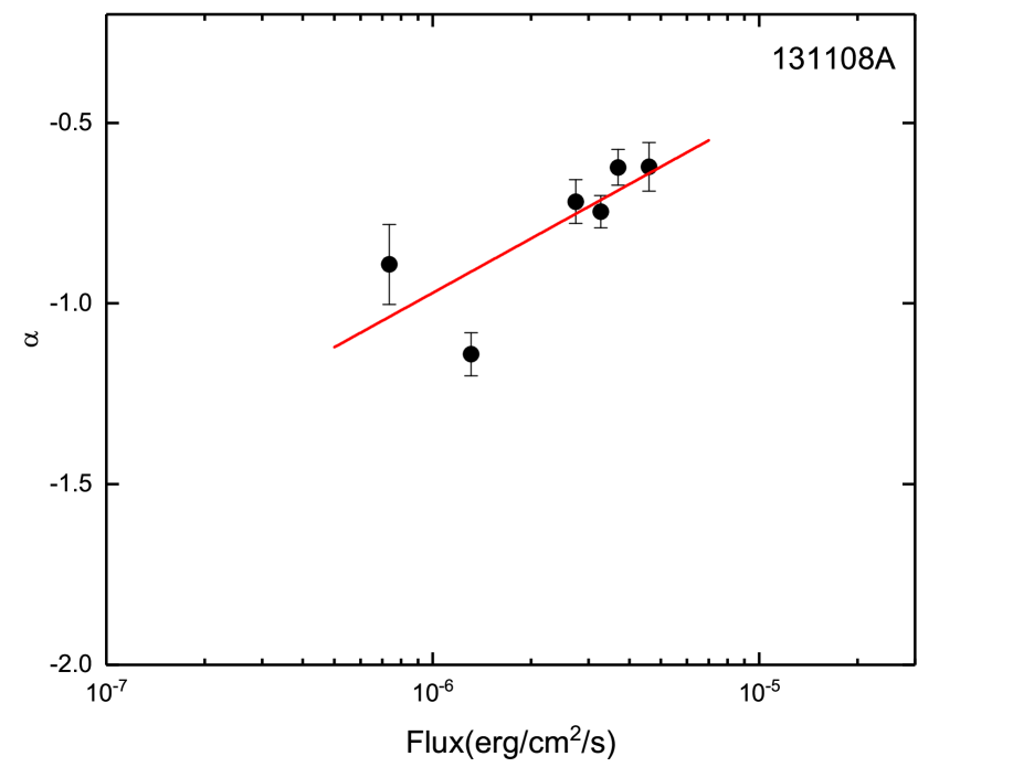
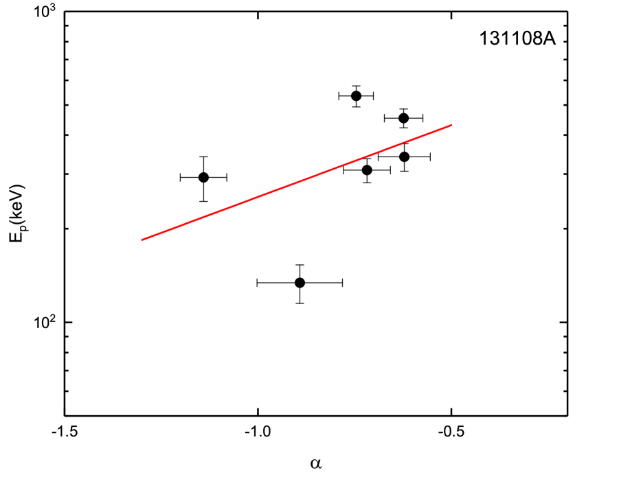
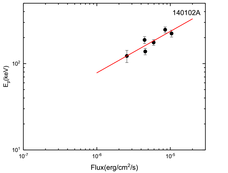
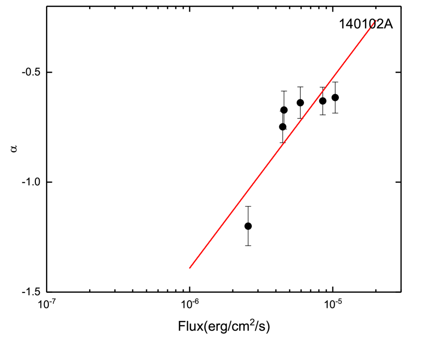
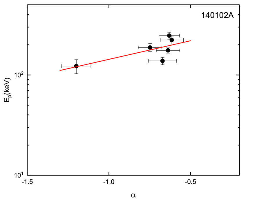
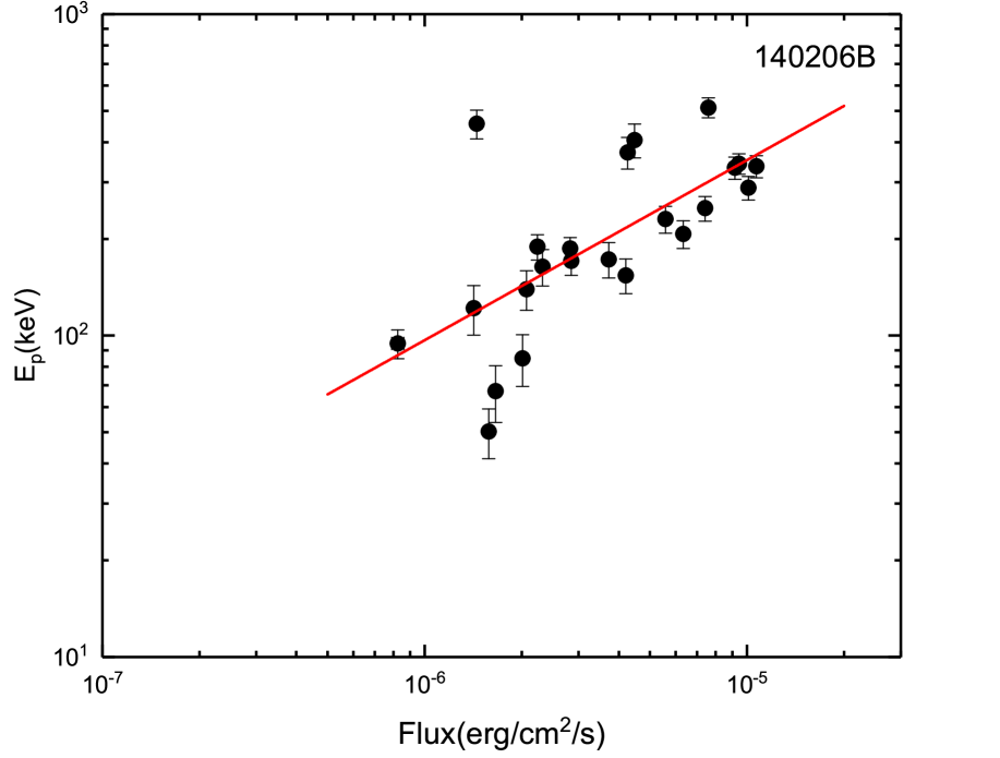
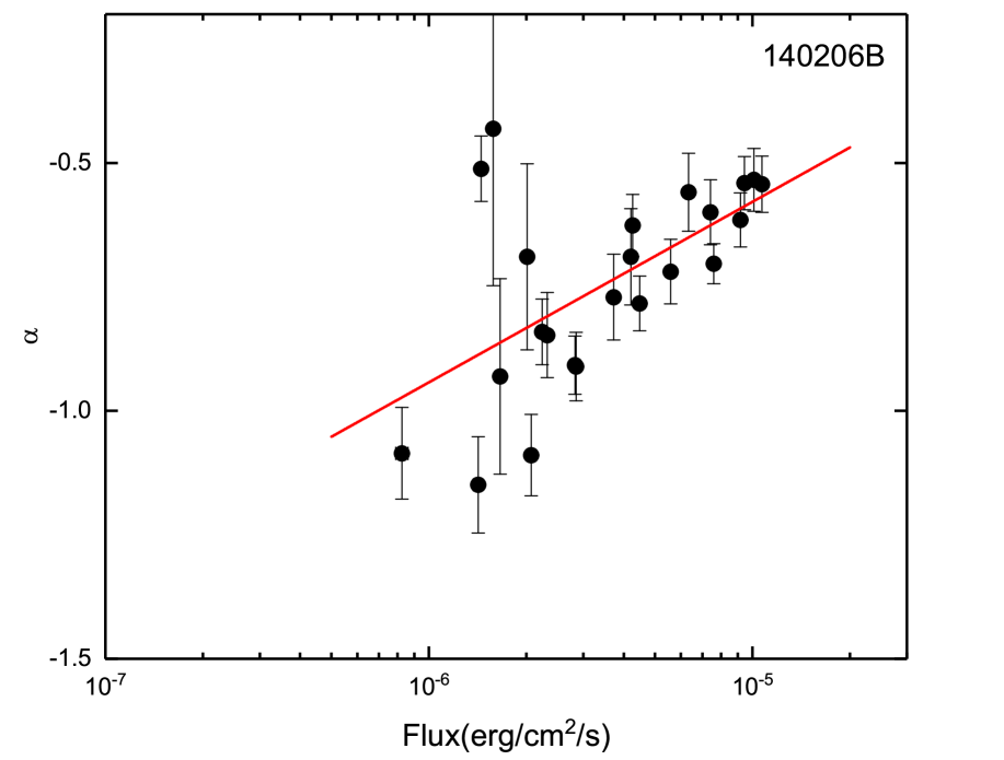
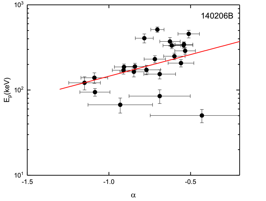
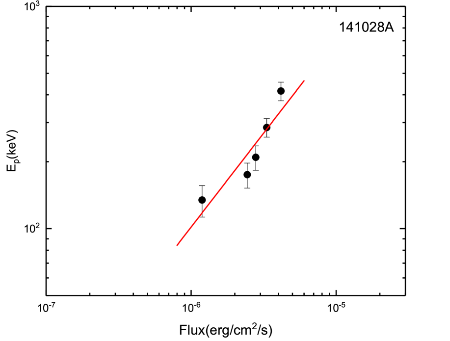
Figure 8: -continued

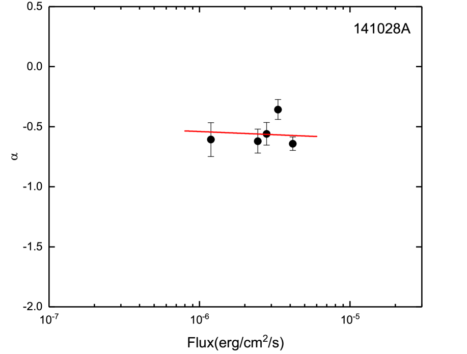
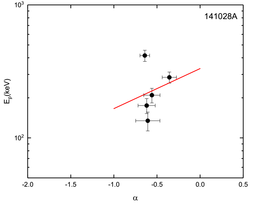
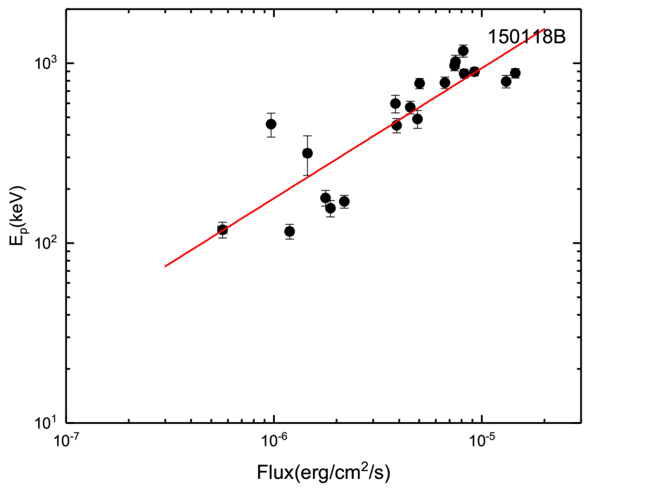
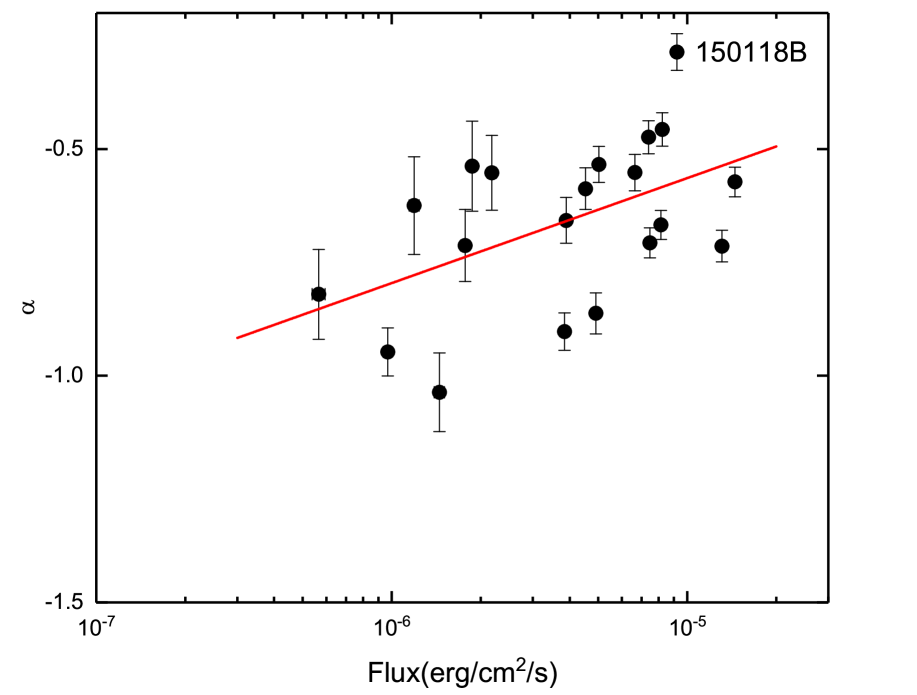
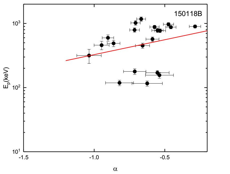
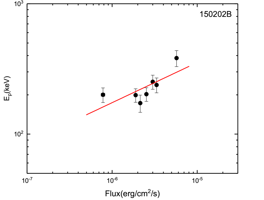
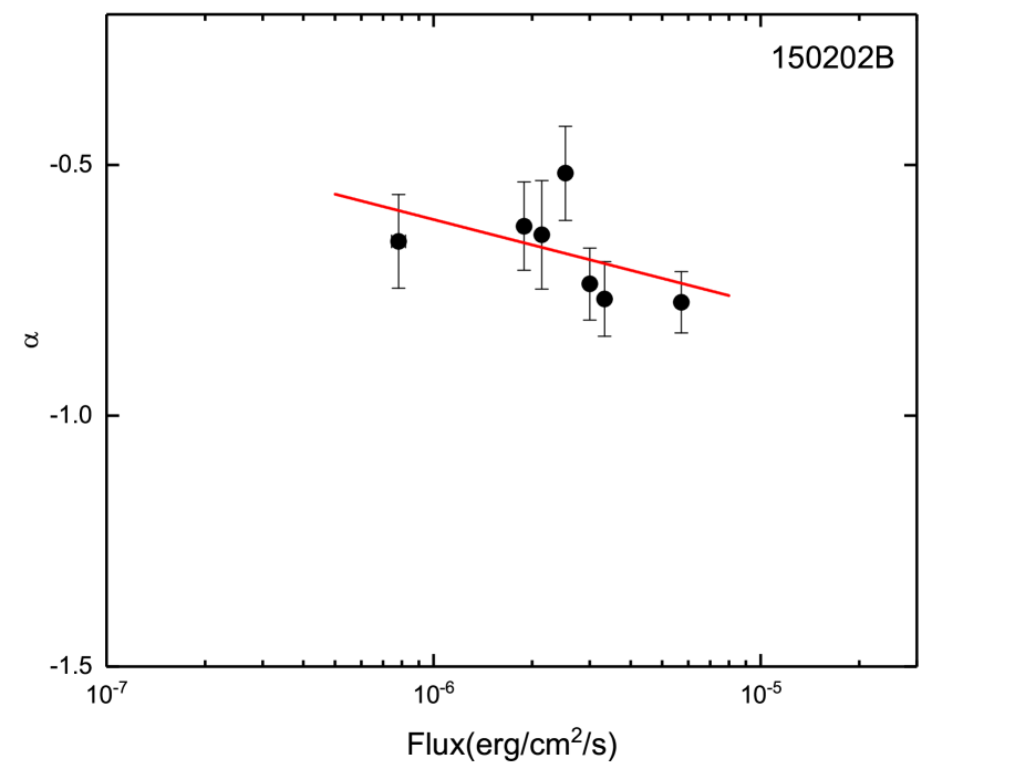
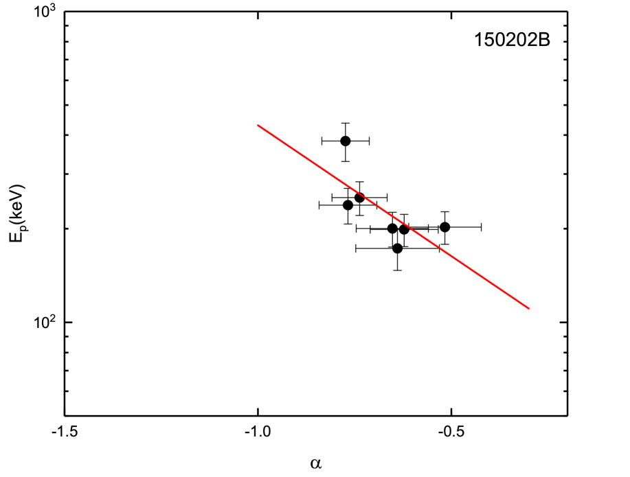
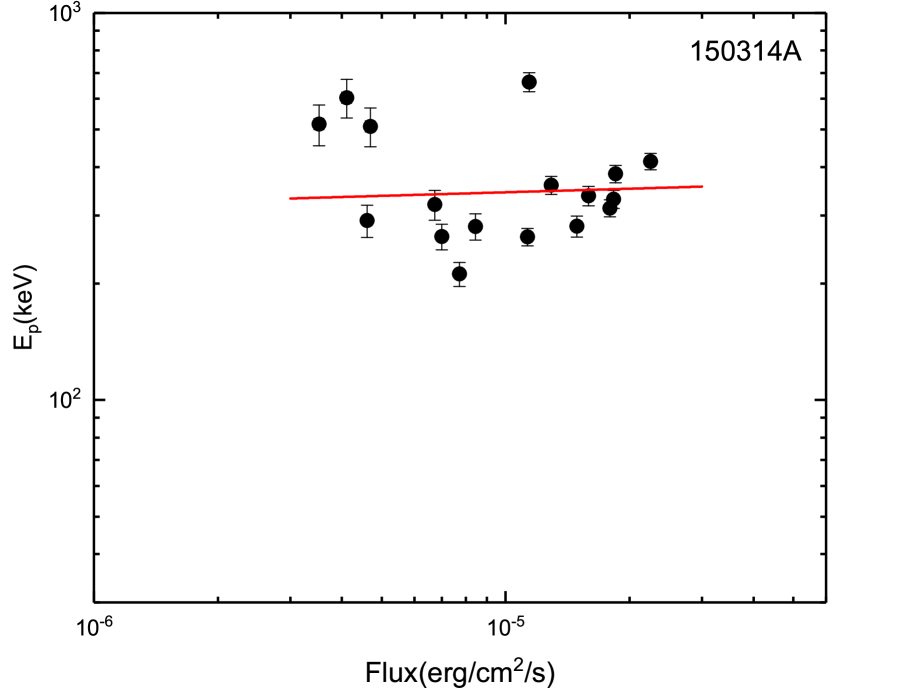
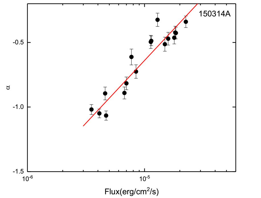
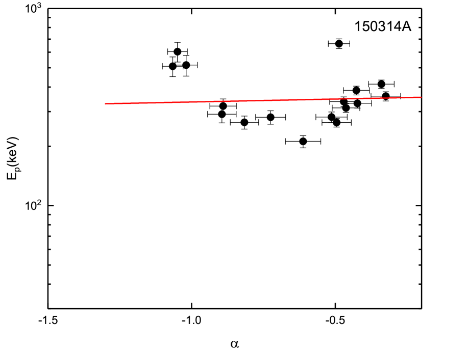
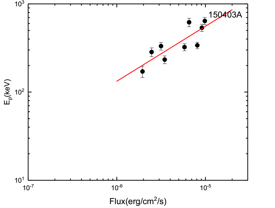
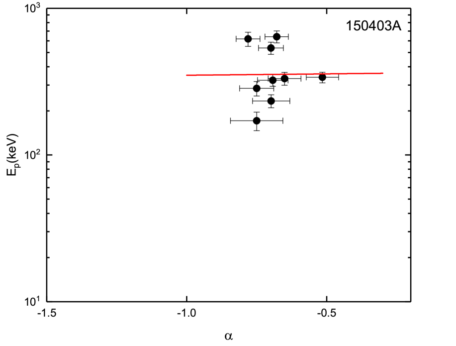
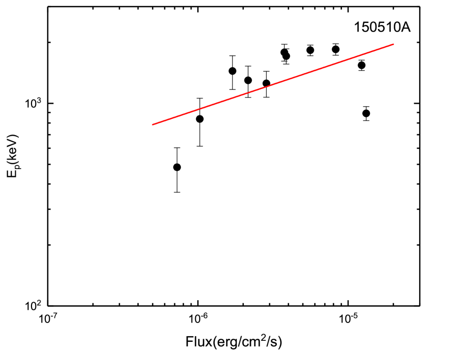
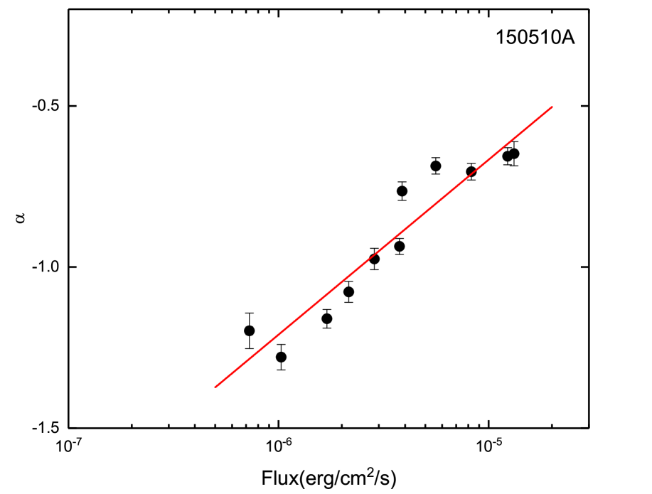
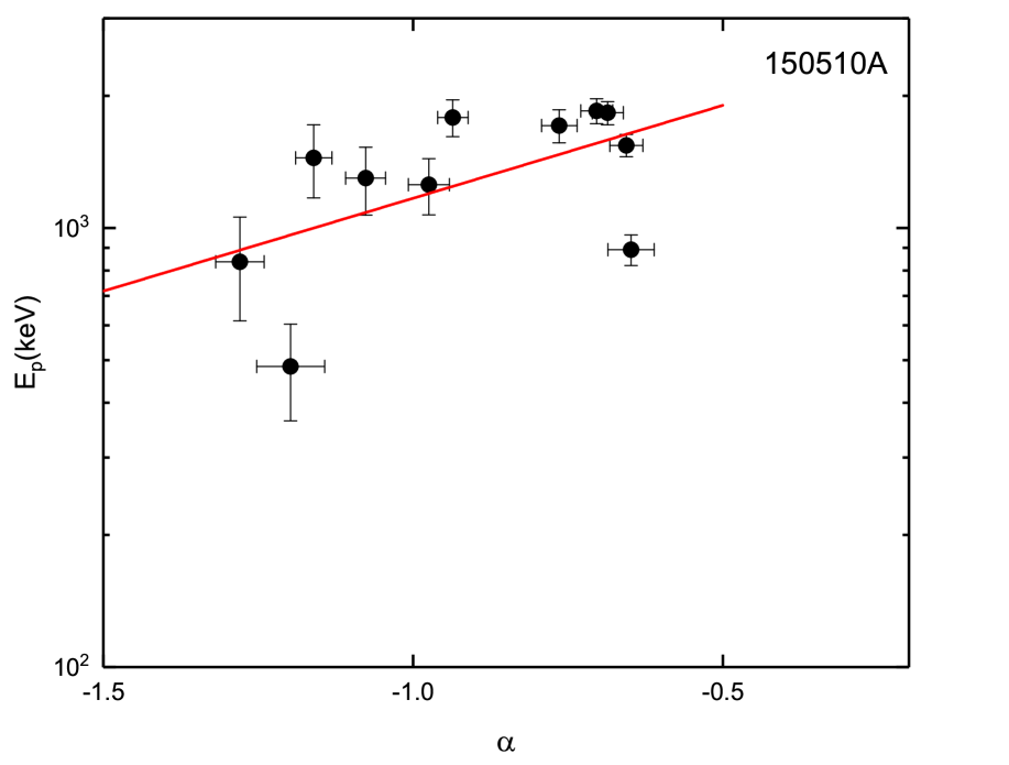
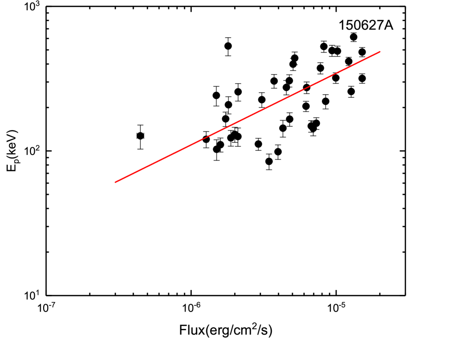
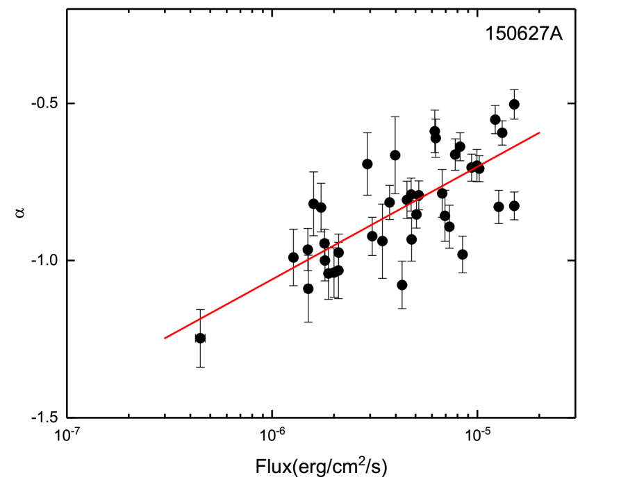
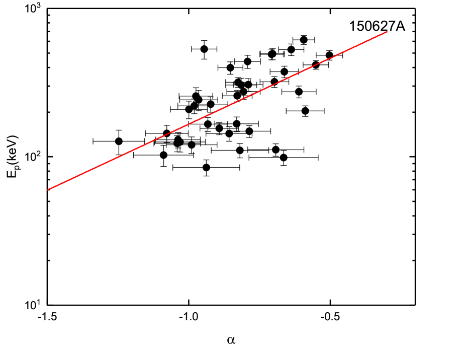
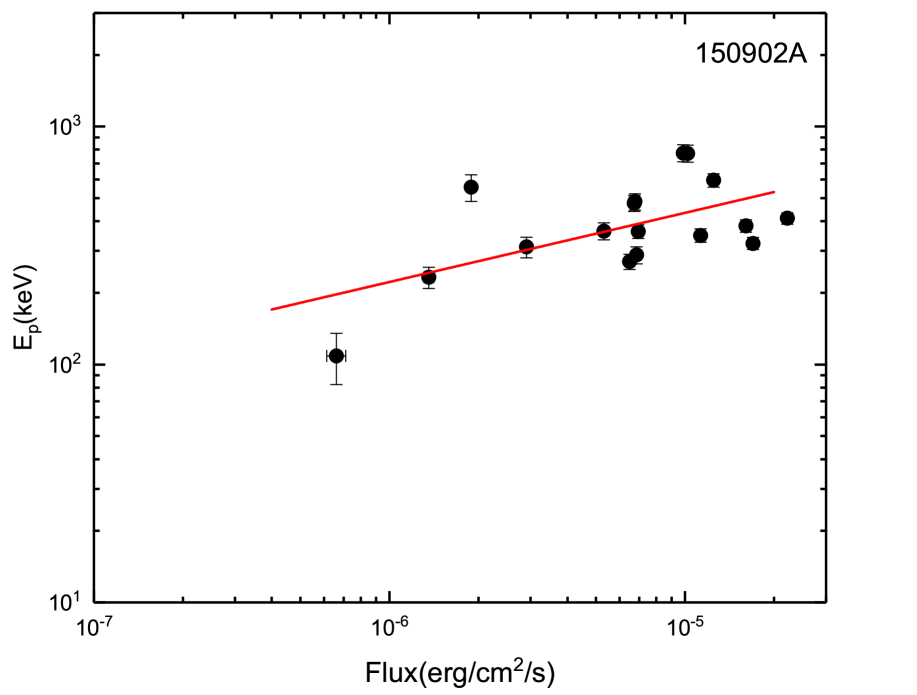
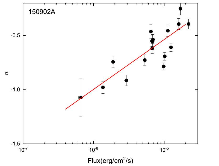
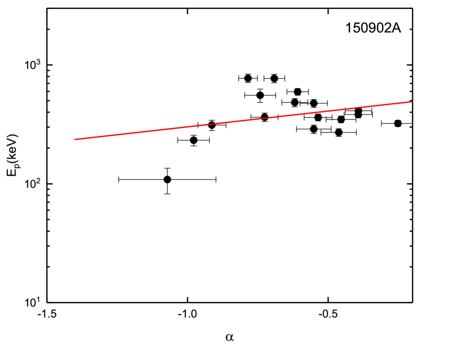
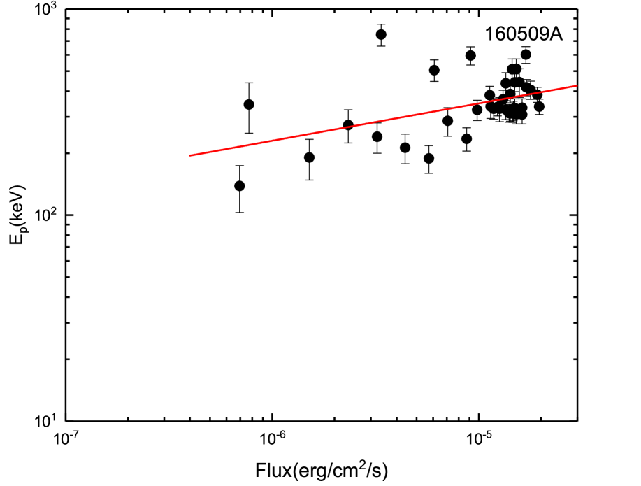
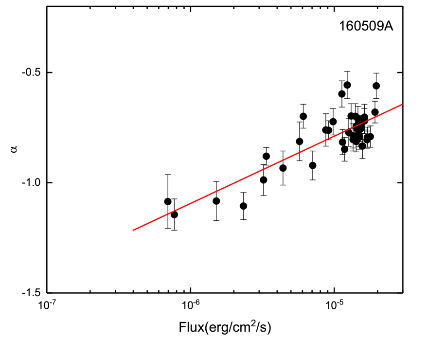
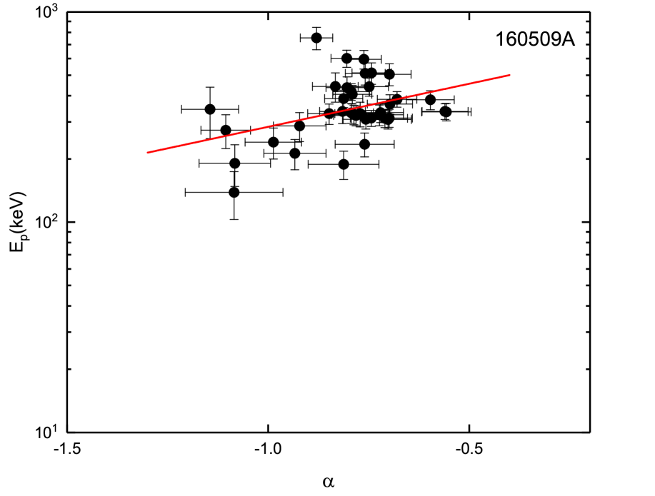
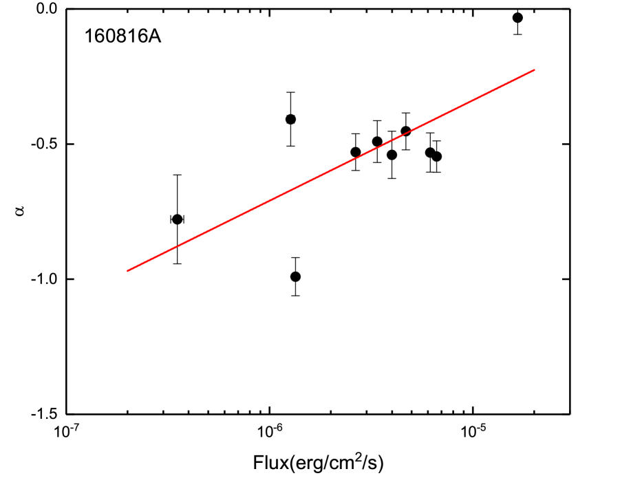
Figure 8: -continued

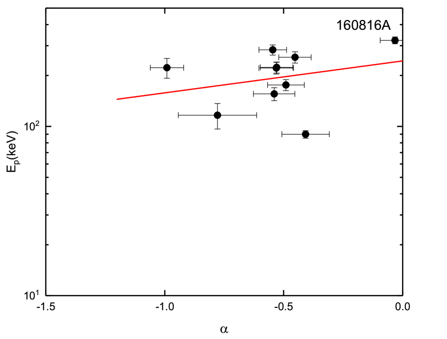
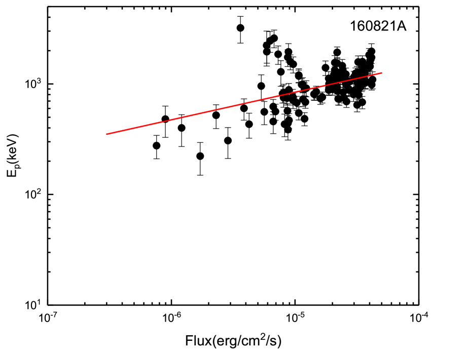
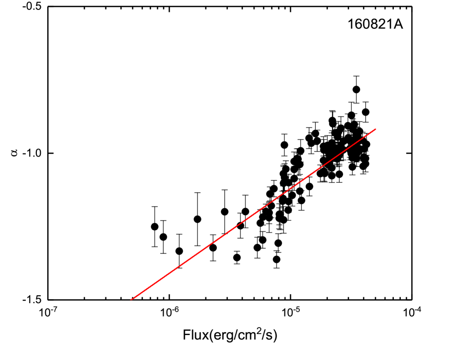
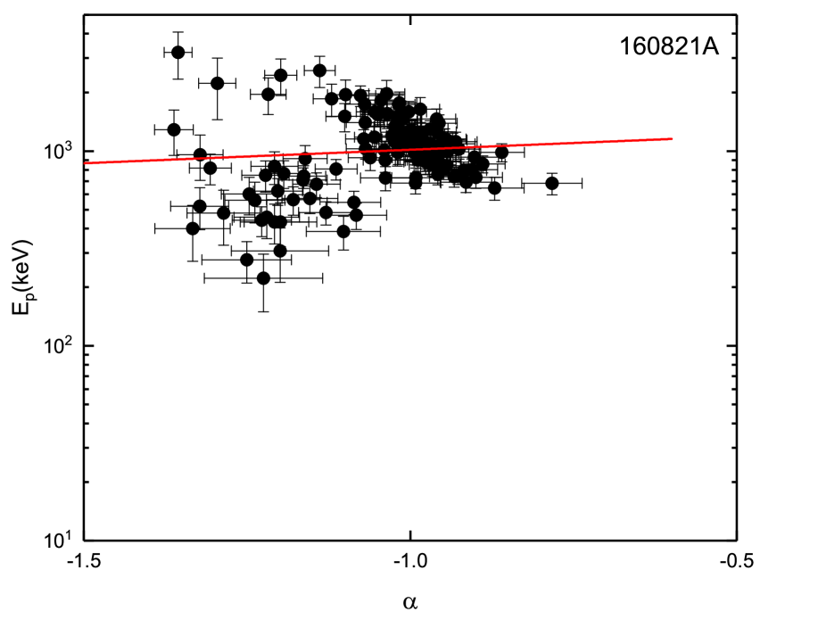
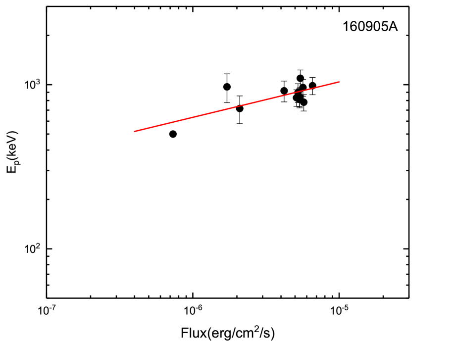
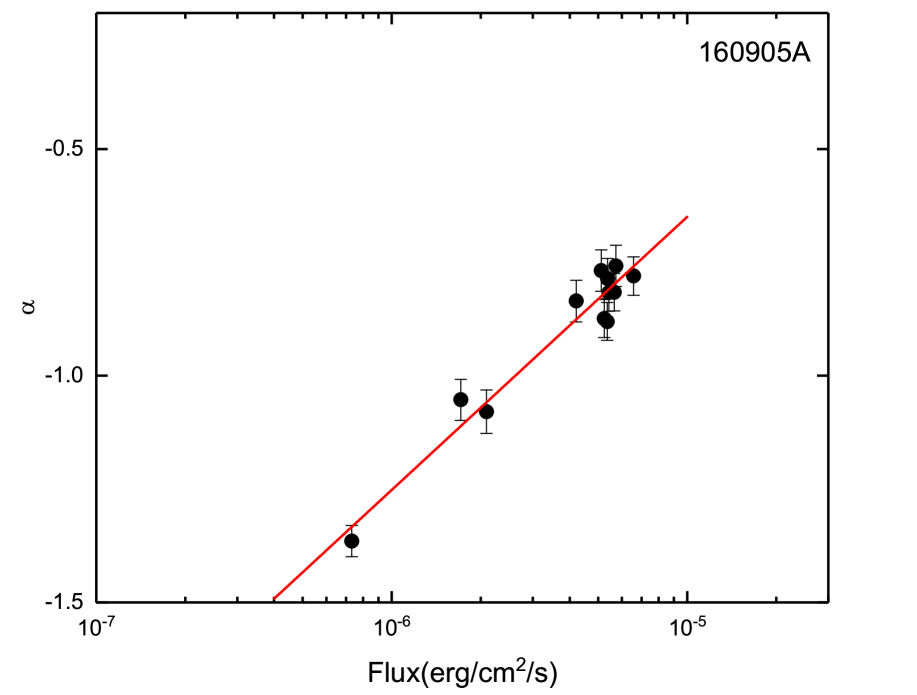
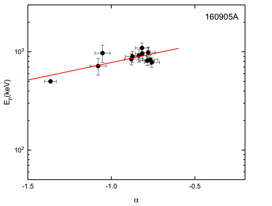
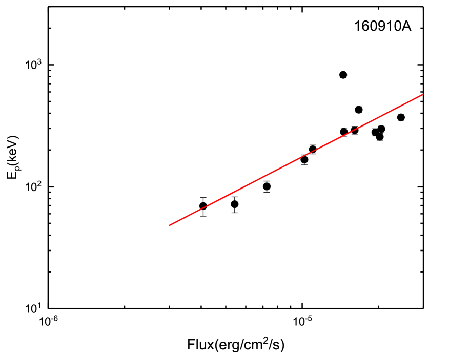
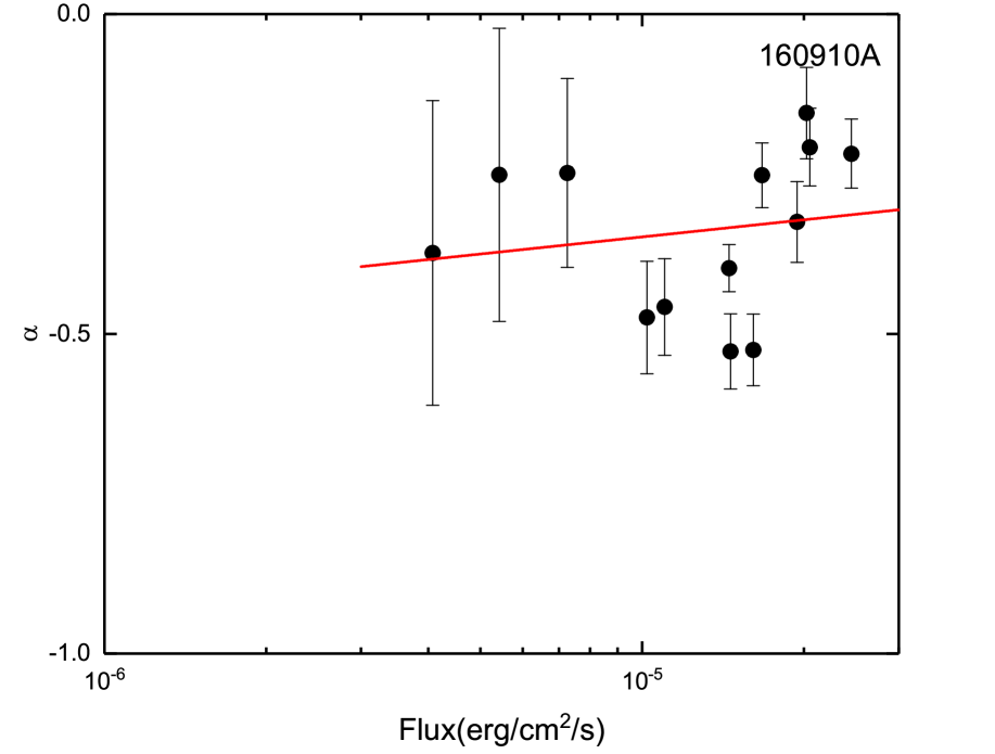
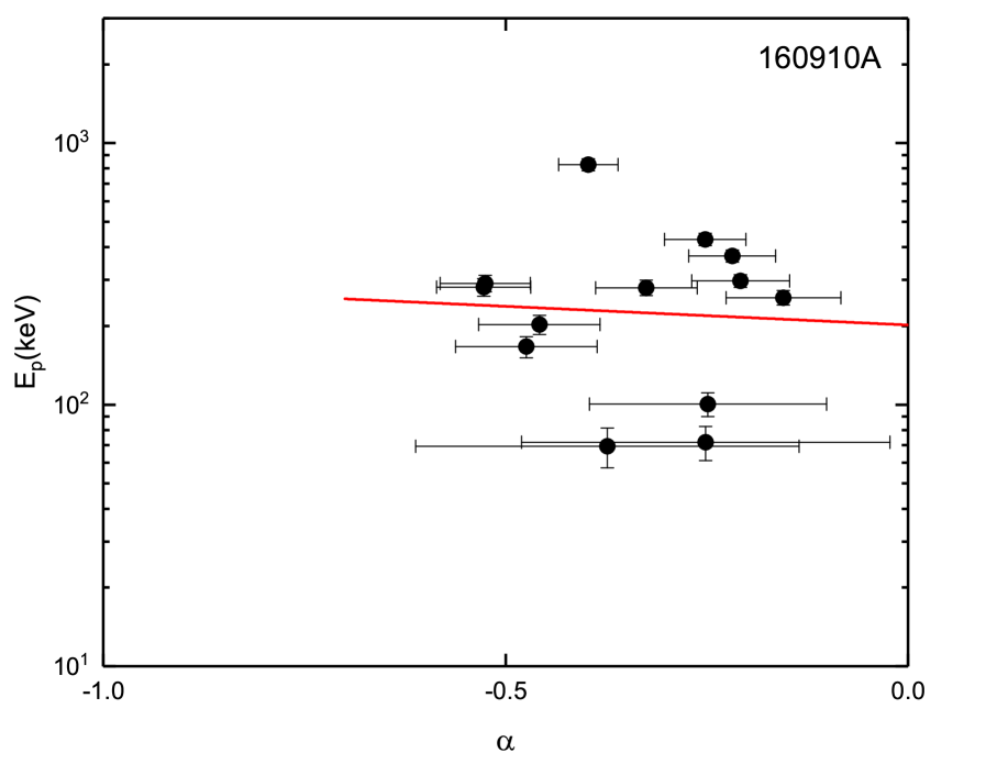
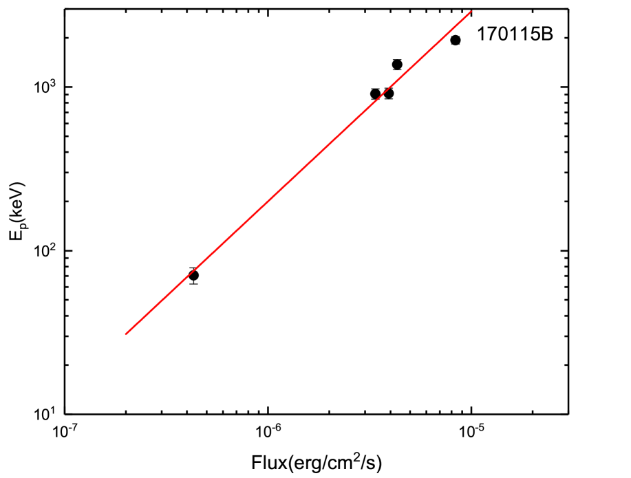
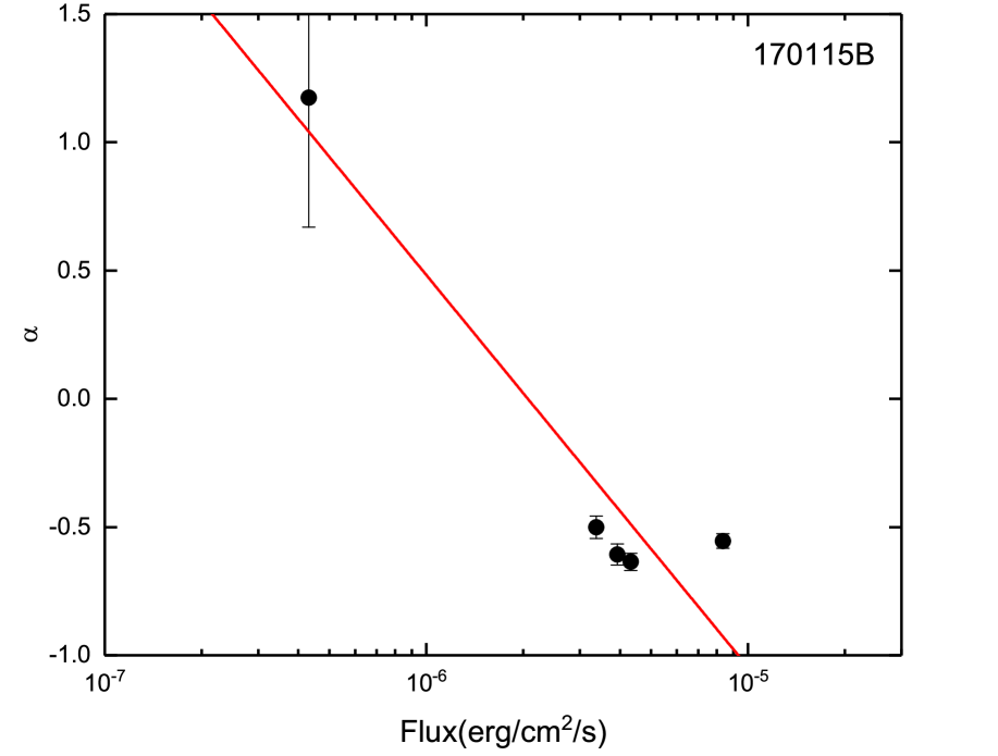
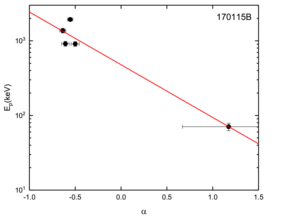
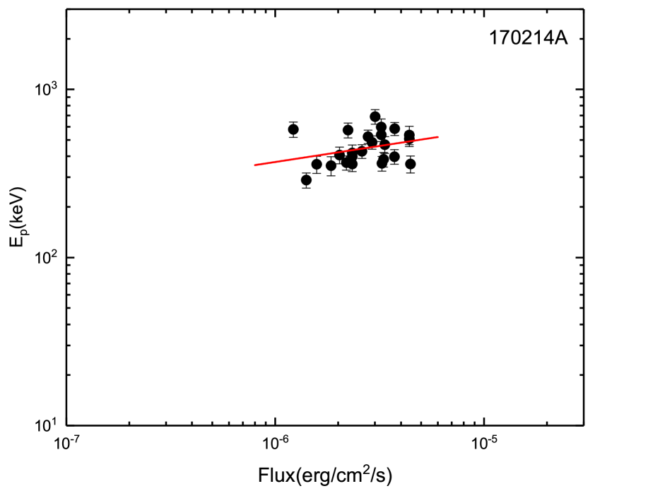
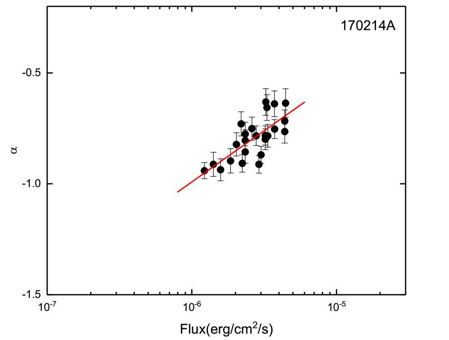
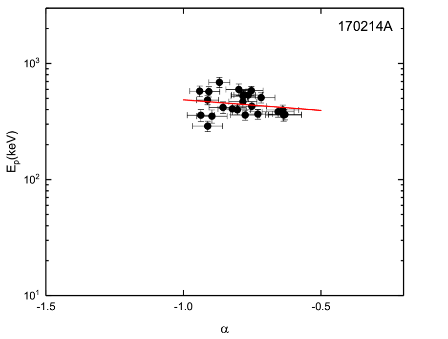
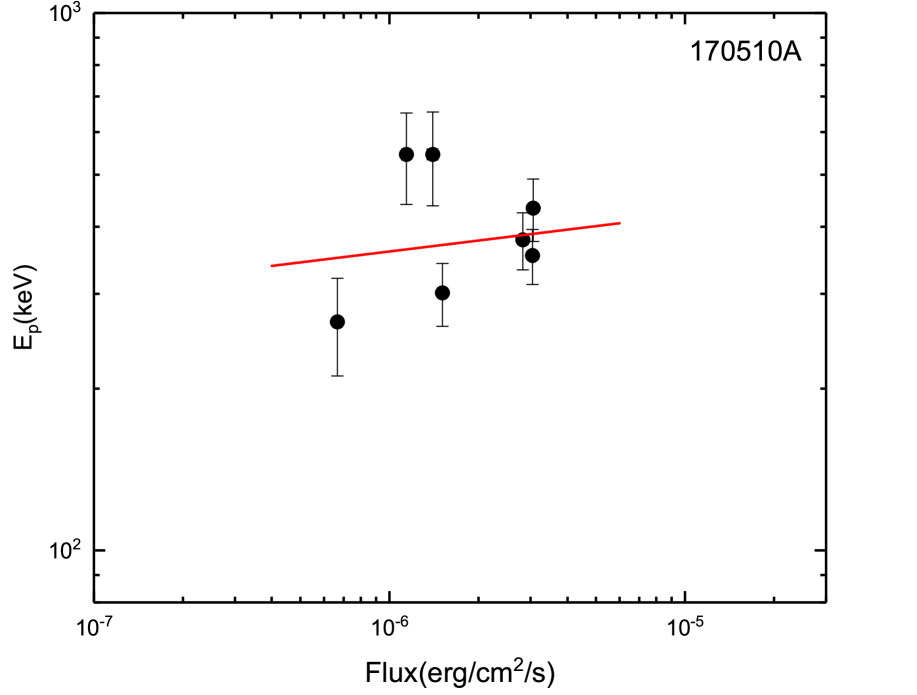
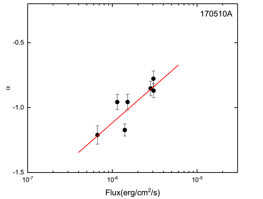
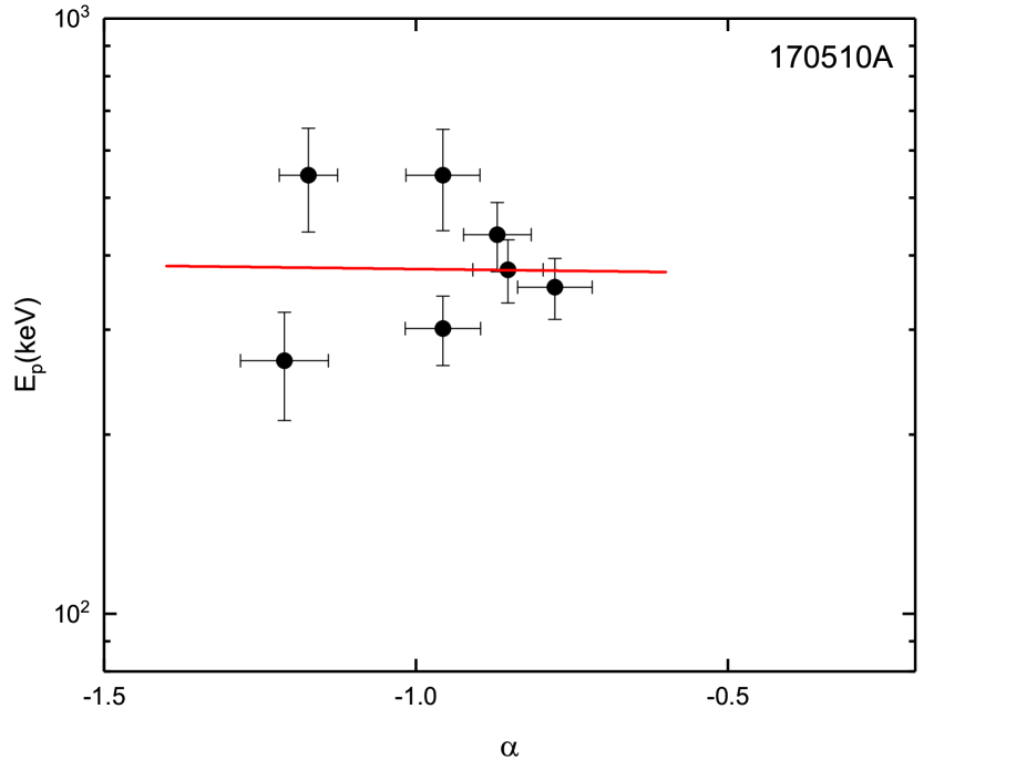
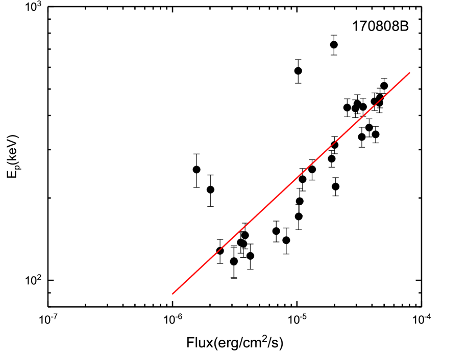
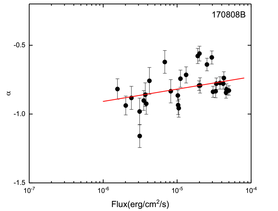
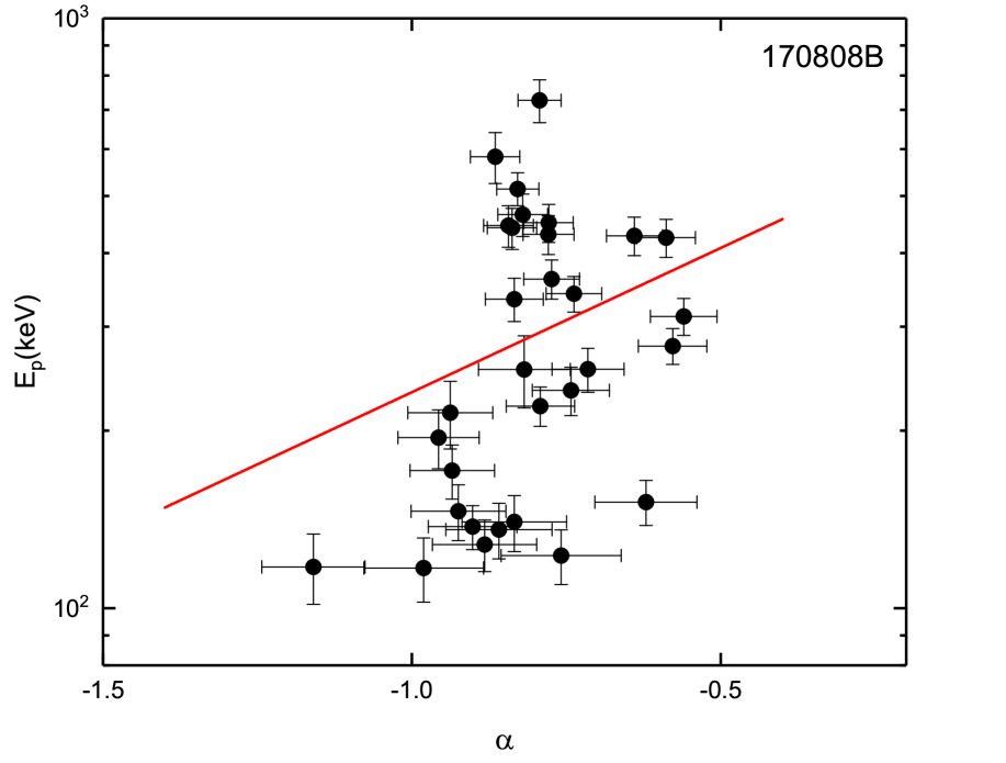
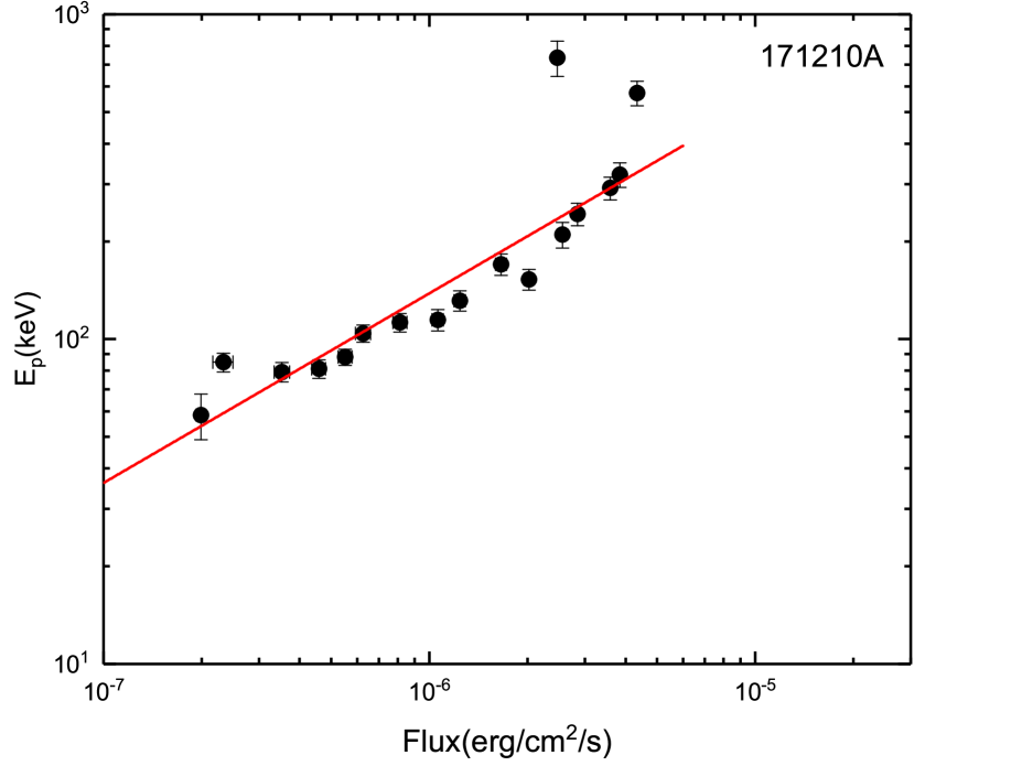
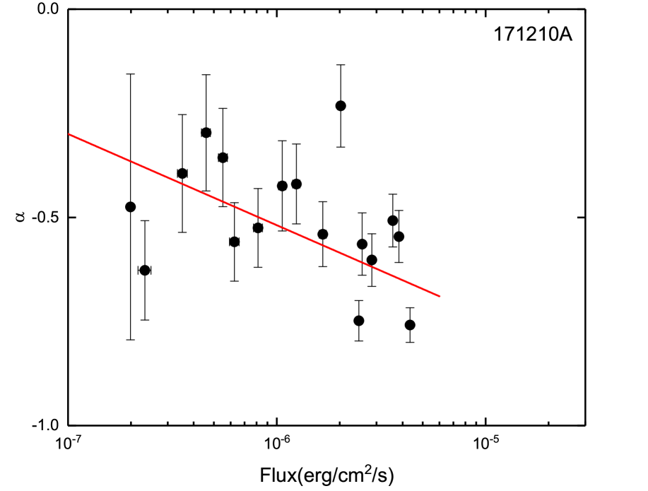
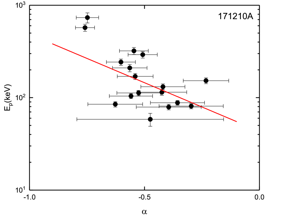
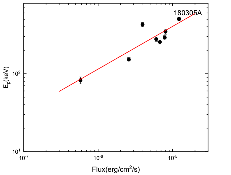
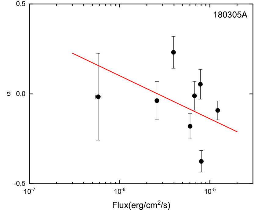
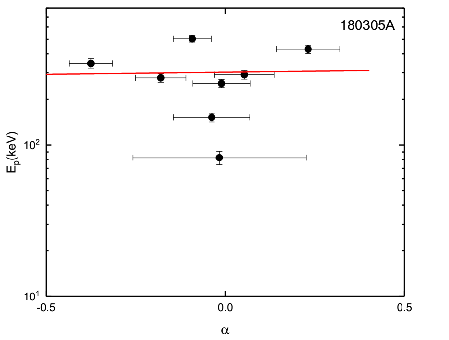
Figure 8: -continued

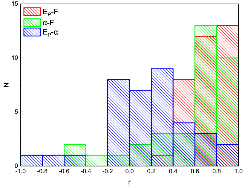
Figure 9: The histograms of Pearson’s correlation coefficient from the fitting results of parameter correlations such as $E_{p}-F$, $\alpha-F$ and $E_{p}-\alpha$. There is a strong monotonous positive correlation both for $E_{p}-F$ and $\alpha-F$ correlations in .

The parameter correlations may play an important role in revealing the nature of the prompt emission for gamma-ray bursts. the correlations such as $E_{p}-F$, $\alpha-F$ and $E_{p}-\alpha$ obtained from the time-resolved spectra are shown in Figure 8 for all of the bursts in our sample. The fitting results of the parameter correlations (Pearson’s correlation coefficient) have been shown in Table 3 (Col.4, Col.5, Col.6) as described in 3.2.2. Figure 9, the histograms of Pearson’s correlation coefficient from the fitting results of parameter correlations such as $E_{p}-F$, $\alpha-F$ and $E_{p}-\alpha$ have been shown on it.

In our analysis, we investigate Figure 8 in detail, then give the fitting results of the parameter correlations (Pearson’s correlation ) in Table 3 the histograms of Pearson’s correlation coefficient from the fitting results of all parameter correlations presented in Figure 9. Those previous analyses such as Borgonovo & Ryde (2001), Firmani et al. (2009), Ghirlanda et al. (2010), Yu et al. (2019) have pointed out that, the $E_{p}-F$ relation (Golenetskii et al., 1983), i.e., the relation between the peak energy $E_{p}$ and energy flux $F$, exhibit three main types: (i) a non-monotonic relation (containing the positive and negative power-law segments while the break occurs at the peak flux); (ii) a monotonic relation which can be described by a single power-law; (iii) no clear trend. For all of our bursts, the most common (in pulses) has a relation described by a single power-law which means that they have a strong positive relation. these, GRBs have a very strong positive relation ($r\in(0.8,1.0)$, see Table 3 and Figure 9) another GRBs have a strong positive relation ($r\in(0.6,0.8)$, also see Table 3 and Figure 9). positive correlation which is not strong or very strong, but the moderate correlation weak correlation (). In a word, of these bursts show strong positive correlation and of show weaker positive correlation compared with the former. However, these results are inconsistent with the study of 38 single pulses in Yu et al. (2019), which shows that 23 single pulses exhibit the non-monotonic relation and 13 pulses exhibit the monotonic relation ( two common in their study).

Turning over to the $\alpha-F$ relation. The study of a large sample of single pulses in Yu et al. (2019) shows a monotonic positive linear relation in the log-linear plots. In the study, the majority of the pulses show strong positive relation (28 pulses), 8 pulses have very strong positive relation and have . However, the results of our study present at least 6 types of monotonic linear relation in the log-linear plots. , ($r\in(0.6,1.0)$). which means that the Pearson’s correlation coefficient is larger than 0.8. ($r\in(0.4,0.6)$). ($r\in(0.2,0.4)$). are different from them in $\alpha-F$ correlation.

Finally, the $E_{p}-\alpha$ correlation differs clearly from the first two relations. 5 GRBs have strong positive relation. Of these bursts, GRBs have a very strong positive relation, GRBs have a general strong positive relation. GRBs have a moderate positive relation and GRBs have a weaker positive relation. . Moreover, one can find that two bursts have a strong negative correlation (GRB 150202B, 170115B). Especially, GRB 150202B has a general strong negative correlation while GRB 170115B has a very strong negative correlation with value of $r=-0.97$.

It is noteworthy that there are two peculiar bursts, GRBs 150202B and 170115B, which have ‘anti-tracking’ compared with energy flux for low energy photon index $\alpha$. The negative correlation exhibits both for their parameter correlations such as $\alpha-F$ and $E_{p}-\alpha$ correlations. The Pearson’s correlation coefficient of $\alpha-F$ is -0.48 for GRB 150202B, which means that a moderate negative correlation, and a strong negative correlation (r=-0.69) has been shown in $E_{p}-\alpha$ correlation for this burst. very strong negative correlation has been exhibited both for $\alpha-F$ (r=-0.95) and $E_{p}-\alpha$ (r=-0.97) correlations for GRB 170115B. Additionally, the fact that the value of $\alpha$ in time-integrated spectrum is smaller than the synchrotron limit while the values of $\alpha$ for all of the slices in time-resolved spectra violate the limit for GRB 170115B can be found.

3.4 Whether the Two Observed Strong Positive Correlations Are Intrinsic or Artificial

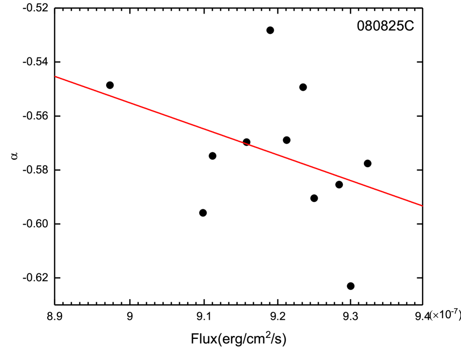
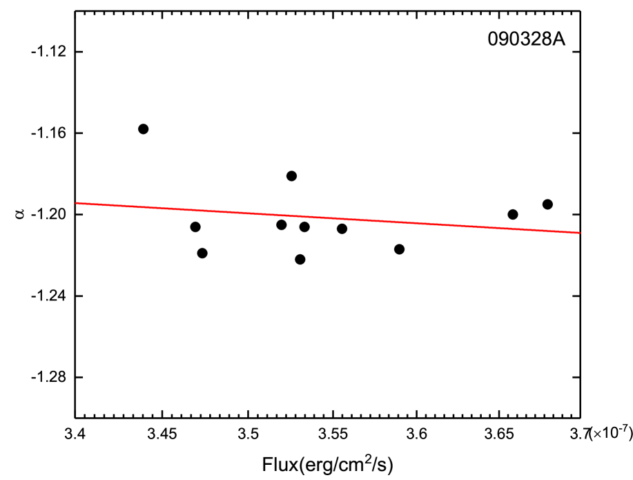
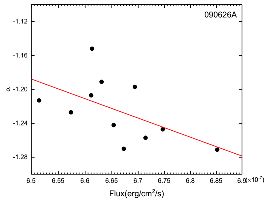
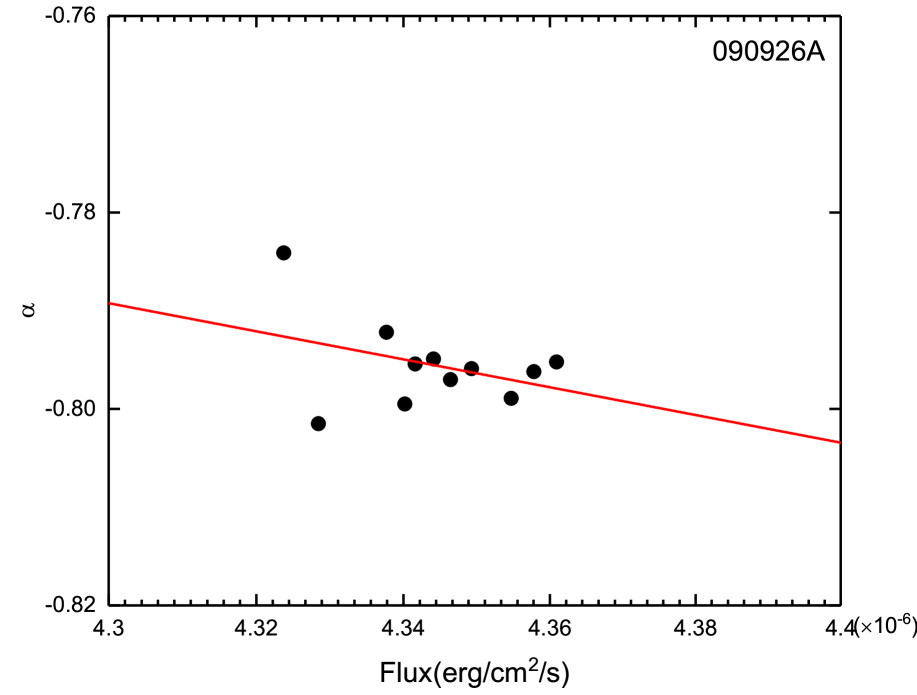
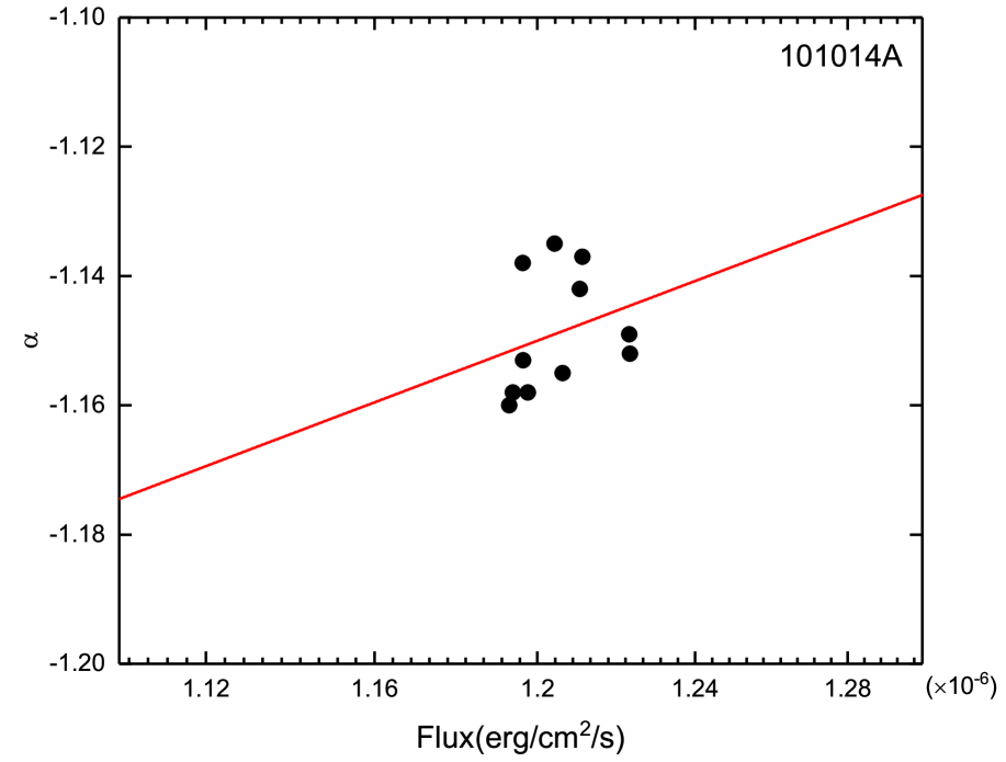
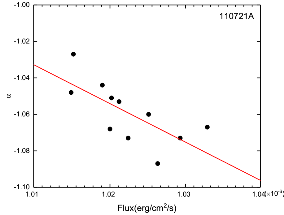
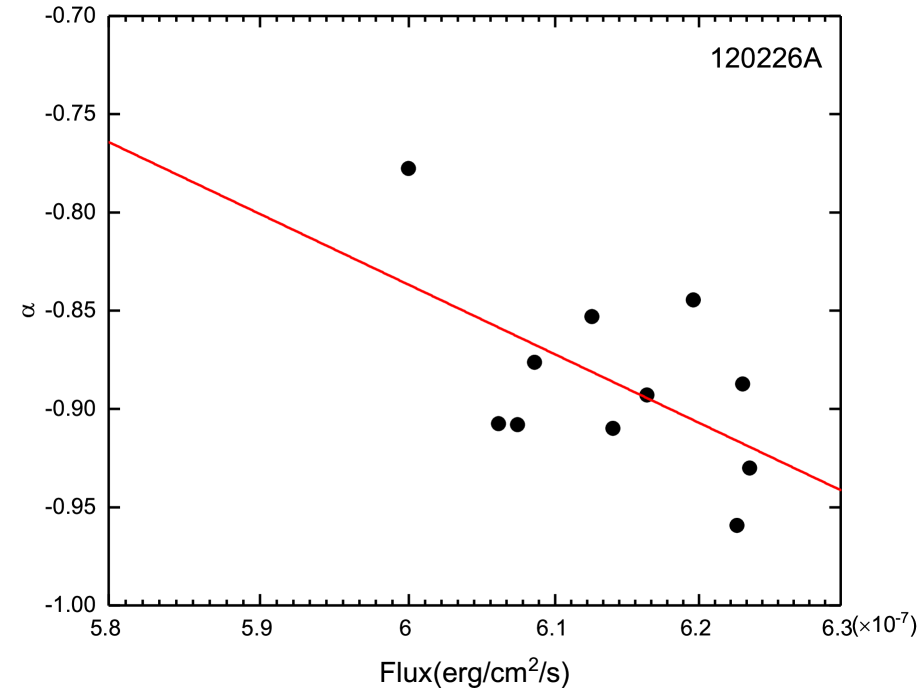
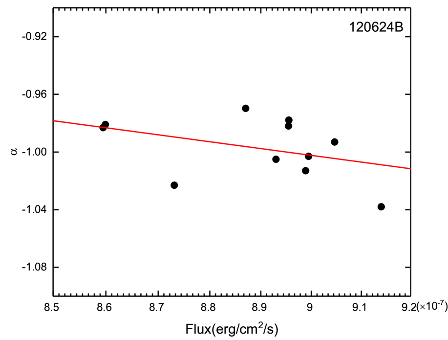
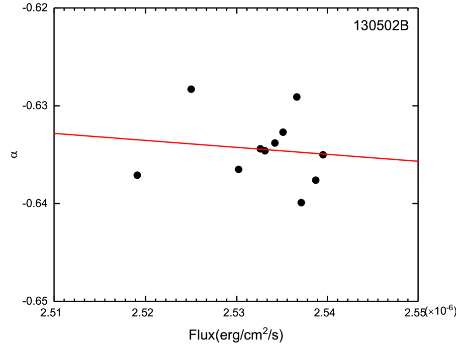
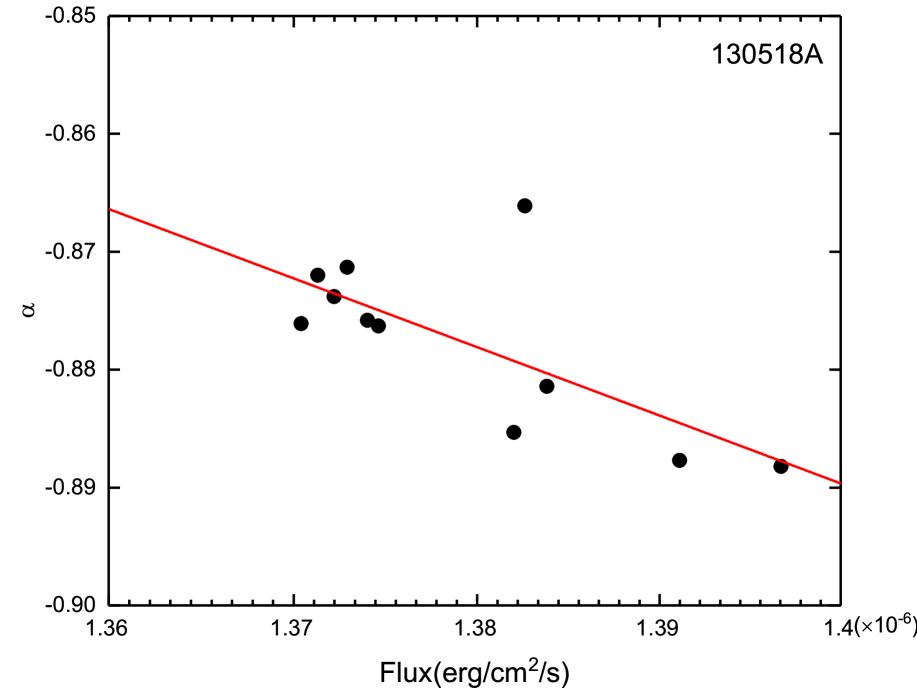
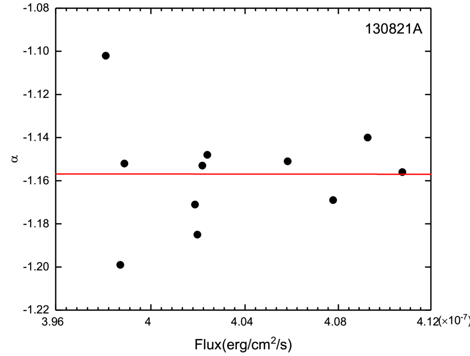
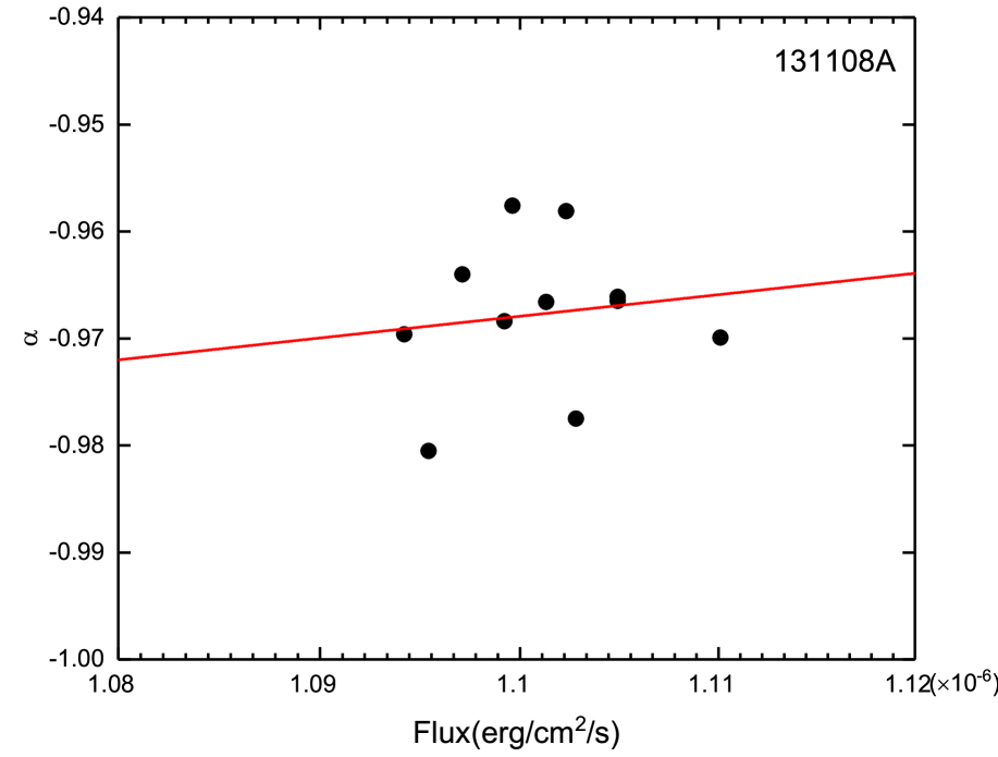
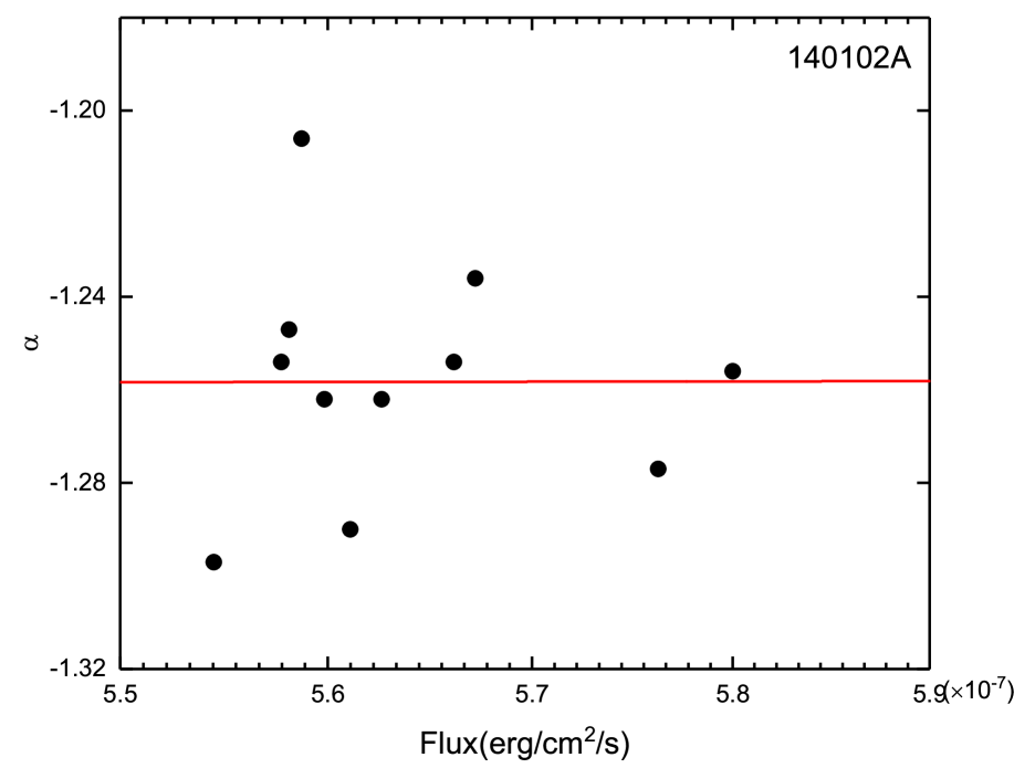
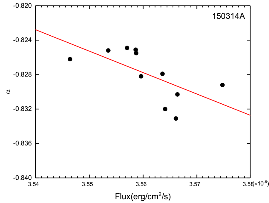
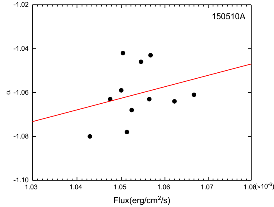
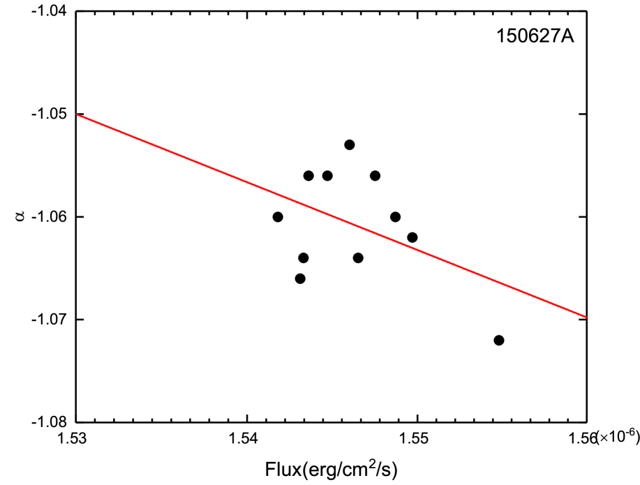
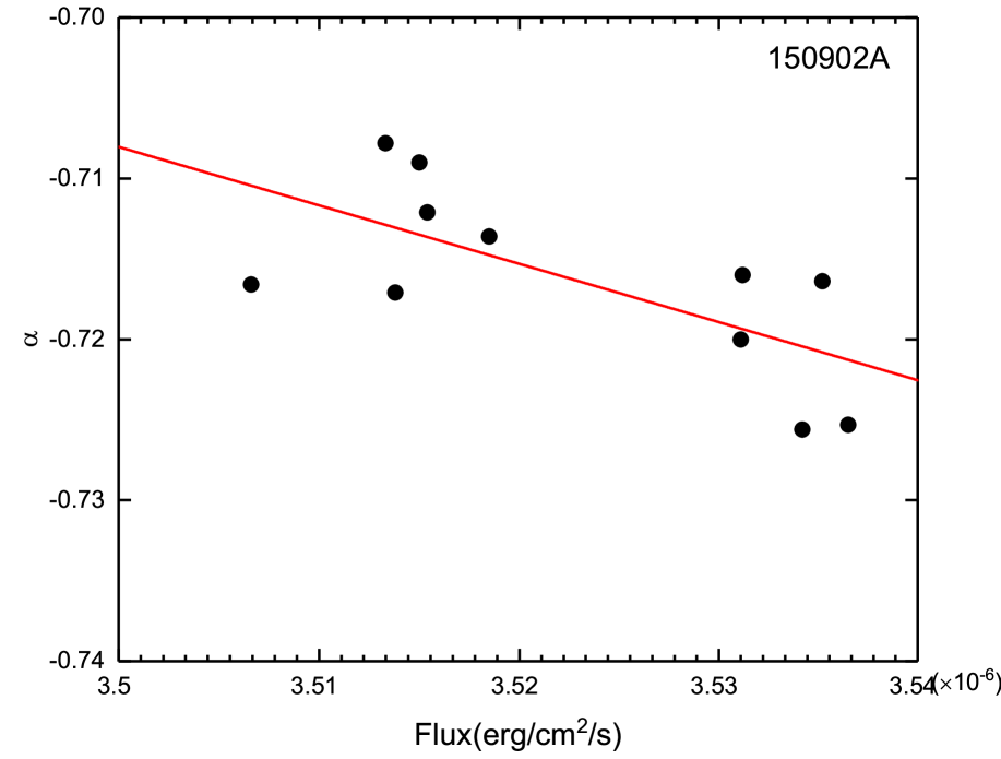
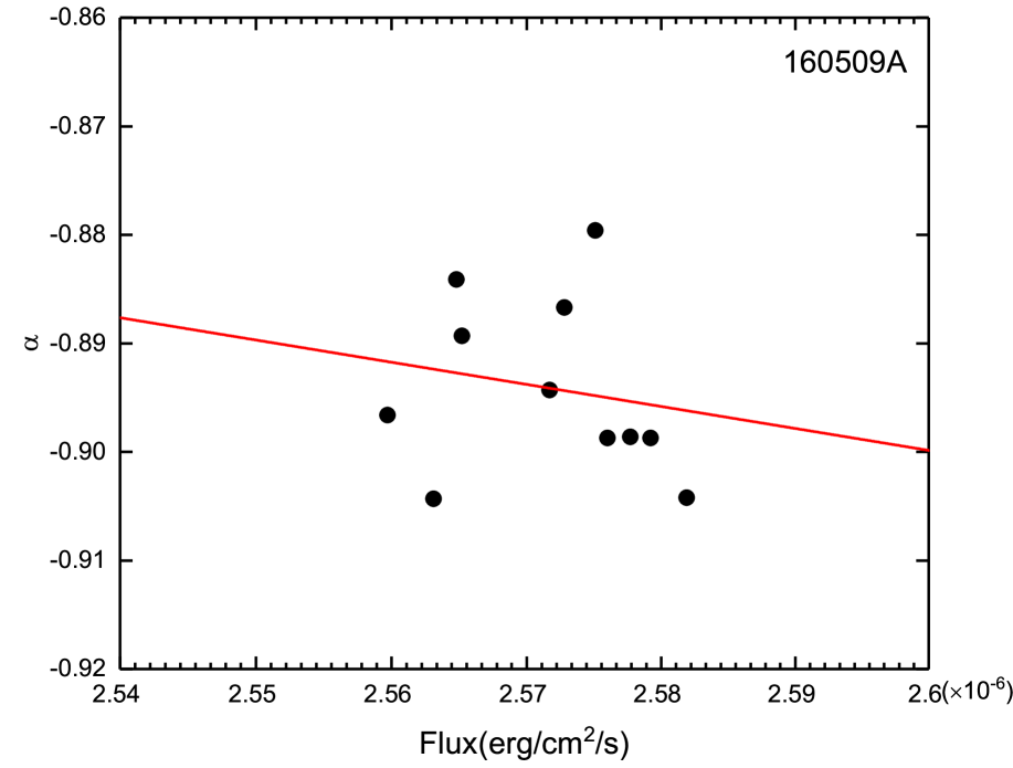
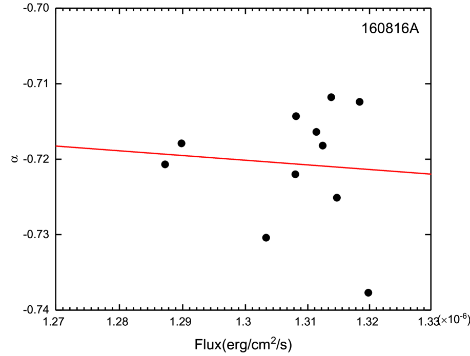
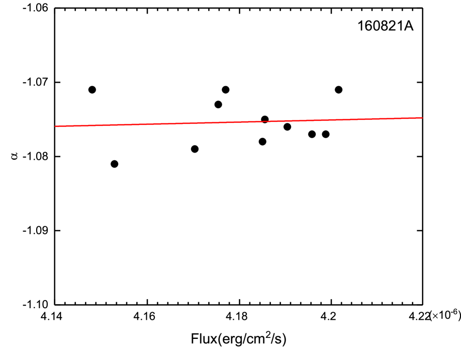
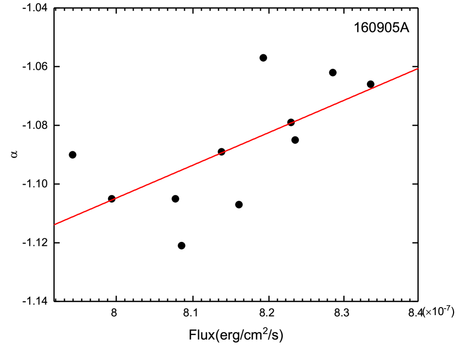
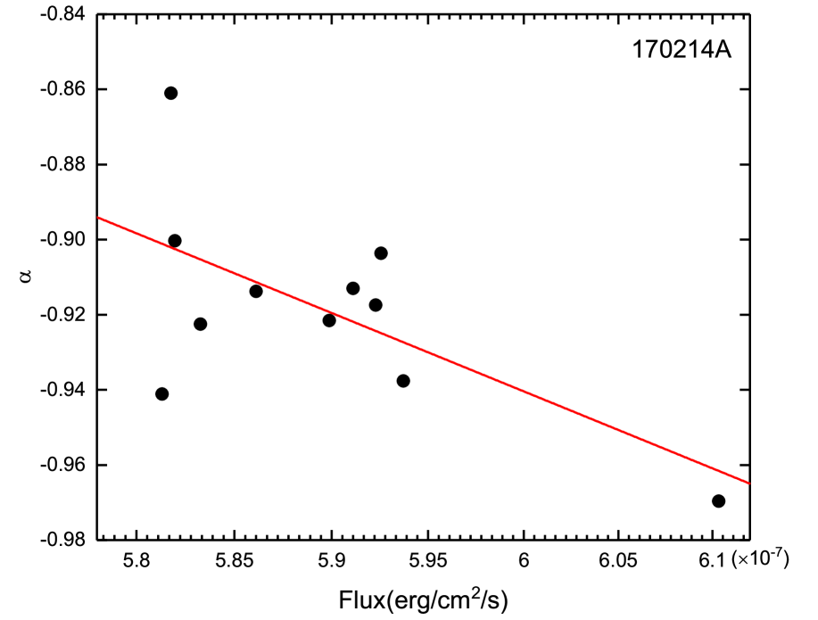
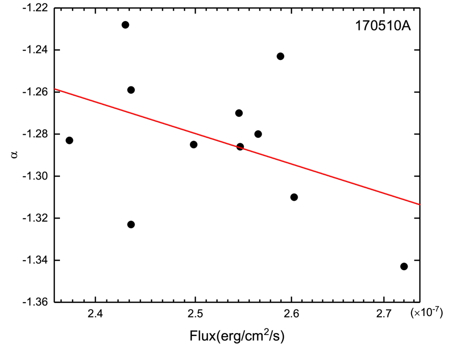
Figure 10:

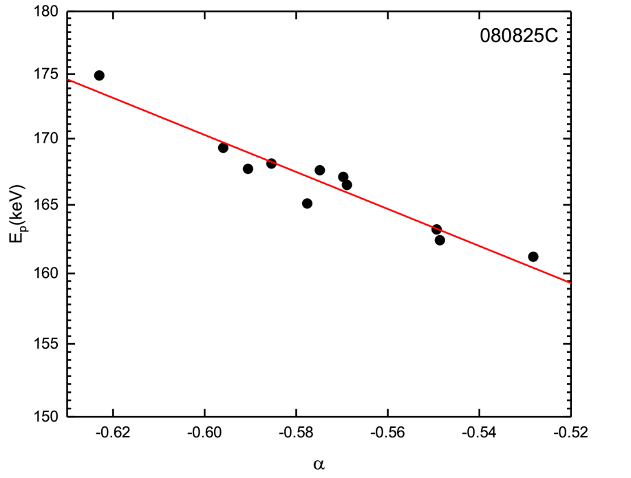
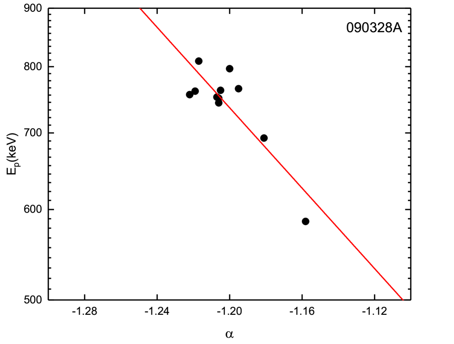
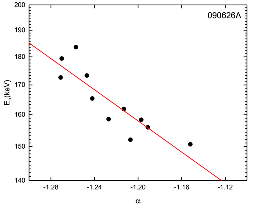
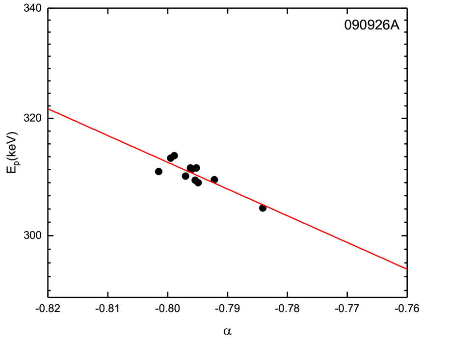
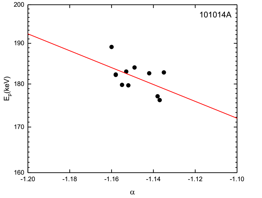
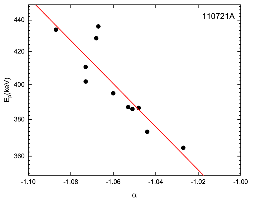
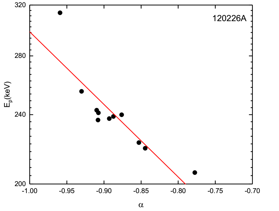
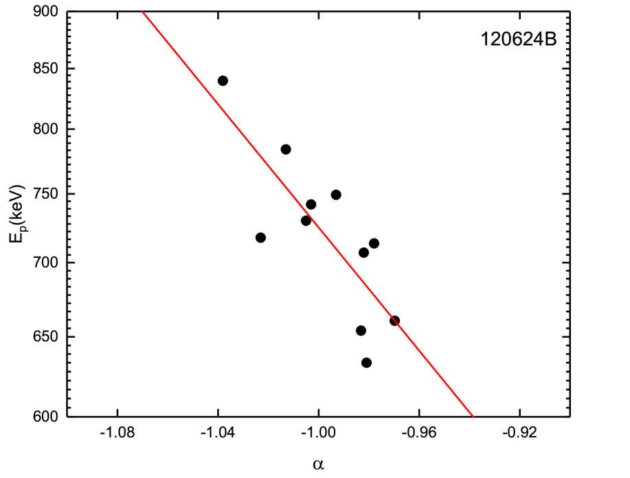
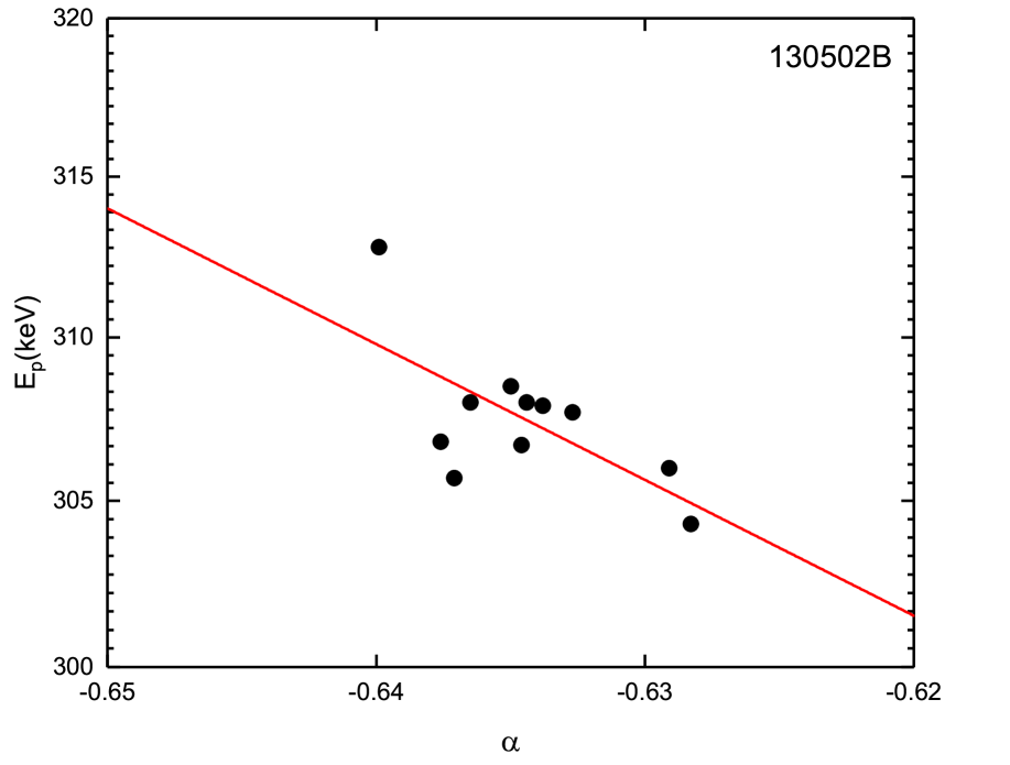
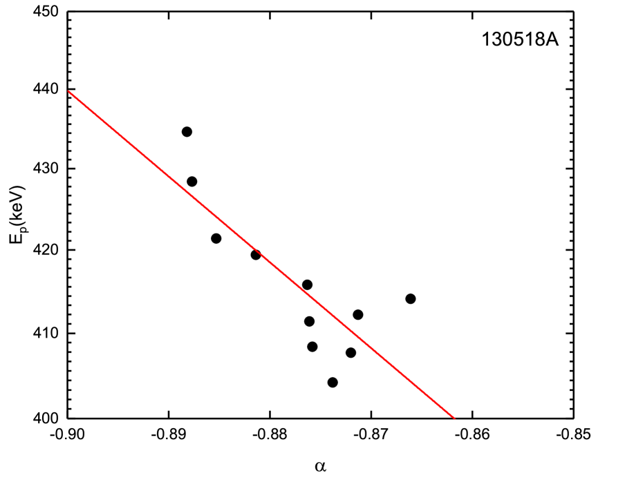
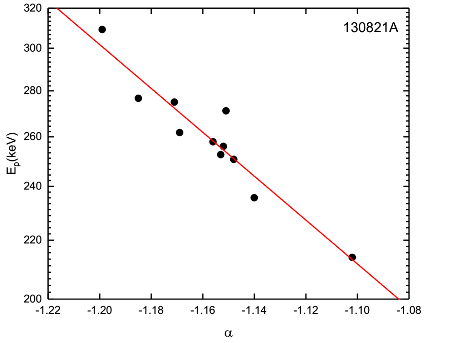
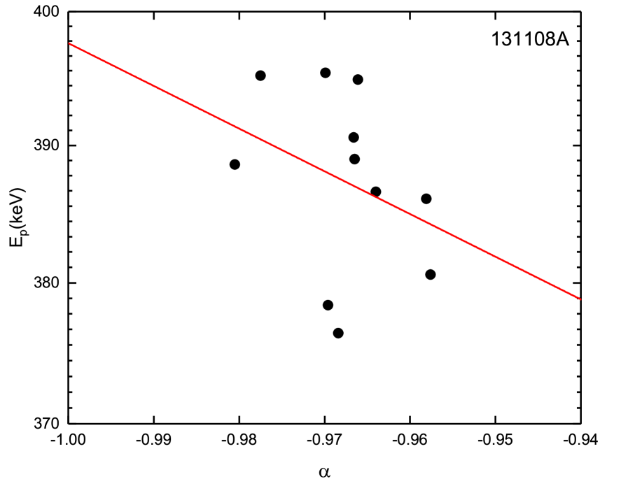
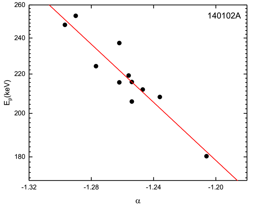
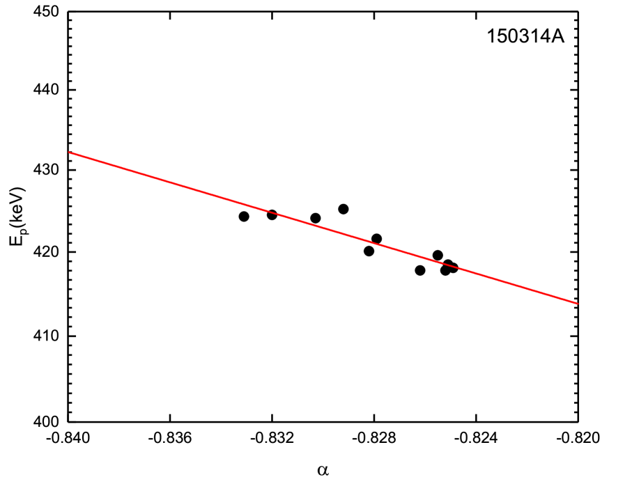
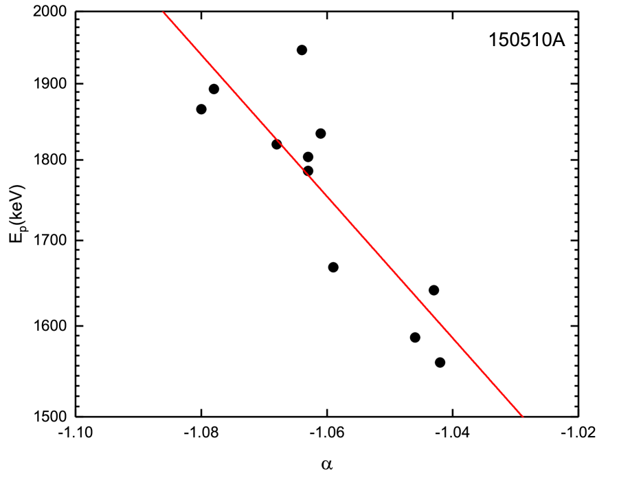
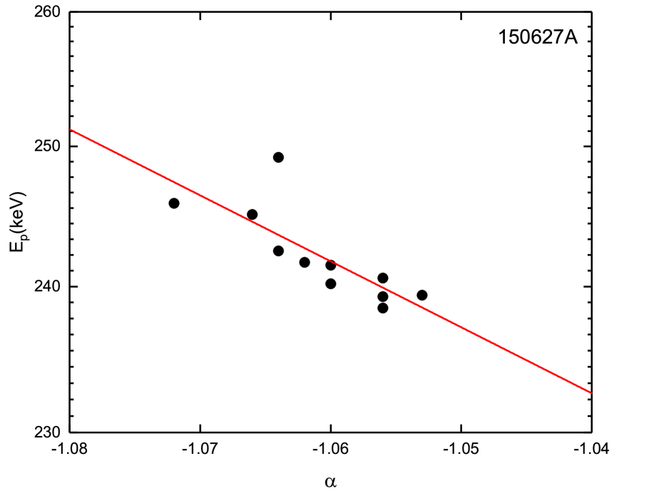
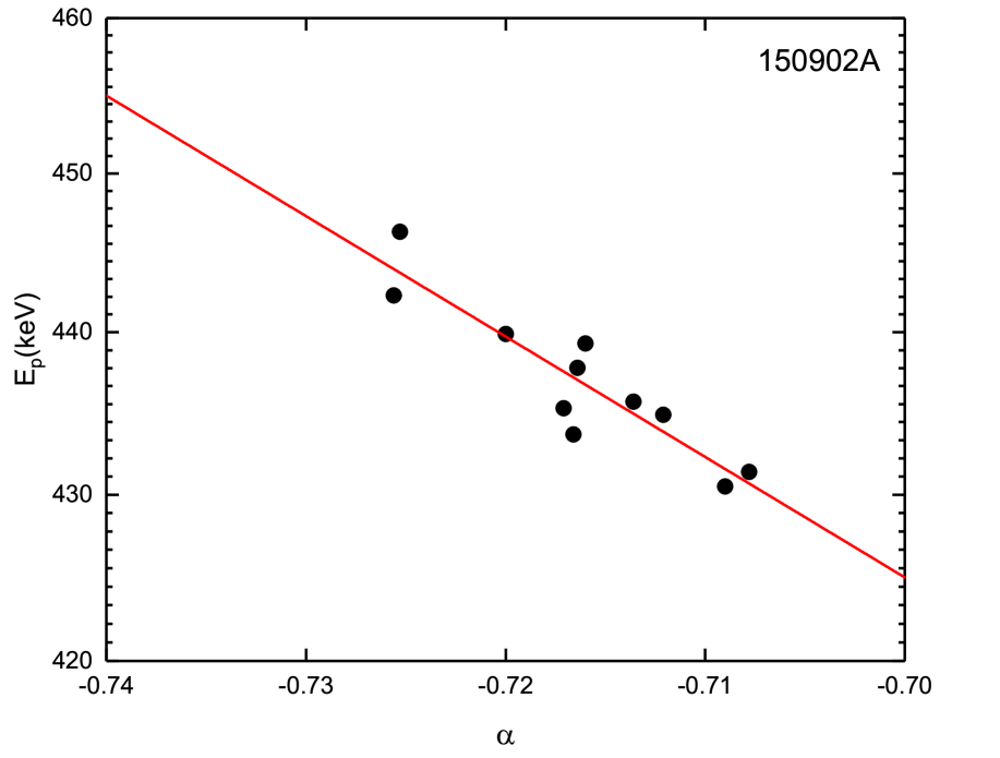
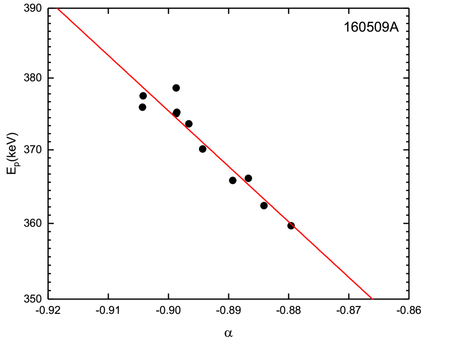
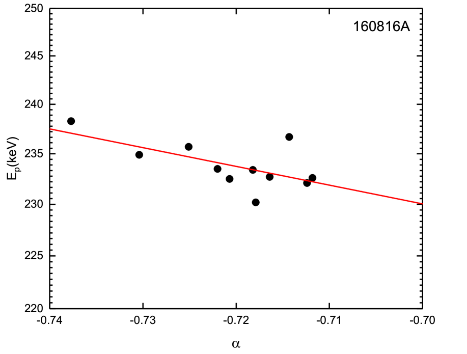
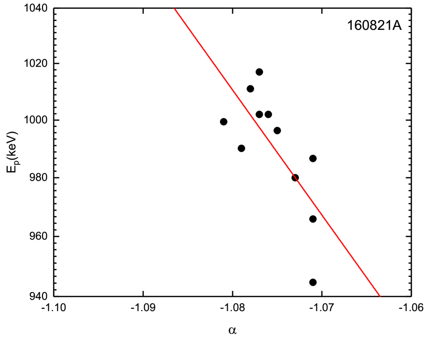
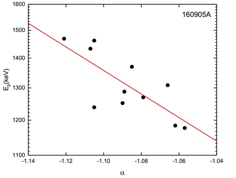
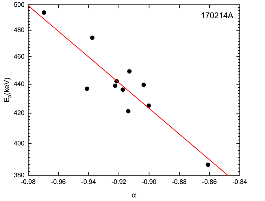
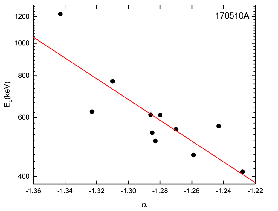
Figure 11:

4 conclusion and Discussion

In this work, after performing the detailed time-resolved analysis of the bright gamma-ray bursts with the detection of $Fermi$-LLE in prompt phase, Then we gave the evolution patterns peak energy $E_{p}$ and low energy spectral index $\alpha$. the parameter correlations such as $E_{p}-F$, $\alpha-F$, and $E_{p}-\alpha$ presented in the analysis.

such as:

1. of the bursts have an $\alpha_{max}$ which is larger than the synchrotron limit ($-\frac{2}{3}$) in our bursts.

2. As we all know, the typical value of low energy photon index $\alpha$ is $\sim-1.0$ for the time-integrated spectrum, while the typical value of $\alpha$ in our sample is .

3. A good fraction of GRBs follow ‘hard-to-soft’ trend (about two-thirds), and the rest should be the ‘flux-tracking’ pattern (about one-third) in the previous literatures for $E_{p}$ evolution. However, it is obvious that the ‘flux-tracking’ pattern is very popular for most of the bursts in our study include ‘intensity-tracking’ ( GRBs) and ‘rough-tracking’ ( GRBs) the total number is , which means that of the bursts exhibit the ‘flux-tracking’ pattern. the low energy photon index $\alpha$ does not show strong general trend compared with $E_{p}$ although it also evolves with time instead of remaining constant in the previous literatures. While, GRBs exhibit ‘flux-tracking’ pattern ‘intensity-tracking’ (2 GRBs) and ‘rough-tracking’ ( GRBs) in our study. In a word, of bursts exhibit the ‘flux-tracking’ pattern.

4. For the parameter correlations, from Section 3.3, a majority of bursts exhibit strong (very strong) positive correlation () between $E_{p}$ and $F$ (energy flux). of bursts have strong (very strong) positive correlation between $\alpha$ and $F$. But there is no clear in $E_{p}-\alpha$ correlation in our sample. , it is noteworthy that very strong negative correlation has been exhibited both for $\alpha-F$ and $E_{p}-\alpha$ correlations for GRB 170115B.

Over the last fifty years, the research in the field of gamma-ray bursts has made a lot of progress, but there are still some open questions (e.g., Zhang, 2011; Dai et al., 2017; Zhang, 2018; Pe’er, 2019). One of the questions is about the radiation mechanism in the prompt emission, which debated whether the GRB prompt emission is produced by the synchrotron radiation or the emission from the photosphere (Vereshchagin, 2014; Pe’Er, & Ryde, 2017). However, a unified model has not been provided even though the physical models like the synchrotron model (Zhang et al., 2016) and subphotospheric dissipation model (Ahlgren et al., 2019) have been used to make the spectral fitting.

As we all know, the Band component in most observed gamma-ray burst spectra seems to be thought as synchrotron origin. Two possible cases should be considered: the first one is for the internal shock model (Paczynski, & Xu, 1994; Rees, & Meszaros, 1994), which invokes a small radius. The second case invokes a large internal magnetic dissipation radius, so-called the Internal-Collision-induced MAgnetic Reconnection and Turbulence (ICMART) model (Zhang, & Yan, 2011). For the internal shock model, the peak energy $E_{p}\propto L^{1/2}\gamma_{e,ch}^{2}R^{-1}(1+z)^{-1}$ can be derived from the synchrotron model in Zhang, & Mészáros (2002), where $L$ is the “wind” luminosity of the ejecta, $\gamma_{e,ch}$ is the typical electron Lorentz factor of the emission region, $R$ is the emission radius, and $z$ is the redshift of the burst. Then, the tracking behavior will emerge because of the natural relation of $E_{p}\propto L^{1/2}$. While a hard-to-soft evolution pattern of peak energy $E_{p}$ is predicted for the ICMART model (Zhang, & Yan, 2011; Uhm, & Zhang, 2014). On the other hand, Uhm et al. (2018) also pointed out that the “flux-tracking” behavior could be reproduced within the ICMART model if other factors such as bulk acceleration are taken into account. Furthermore, Zhang et al. (2016) demonstrated that the synchrotron model can reproduce the $E_{p}$-tracking pattern through the data analysis for GRB 130606B. Therefore, the “flux-tracking” behavior of $E_{p}$ can be made with both these two synchrotron models. In a short, a hard-to-soft pattern and tracking behavior of $E_{p}$ can be reproduced successfully in the synchrotron model.

Meanwhile, the photosphere model can also produce an $E_{p}$-tracking pattern and a hard-to-soft pattern of $E_{p}$ successfully (Deng & Zhang, 2014; Meng et al., 2019). But, this model predicts a hard-to-soft pattern of $\alpha$ instead of $\alpha$-tracking behavior. It is difficult to produce the observed $\alpha$-tracking behavior in this model. On one hand, the predicted $\alpha$ value ($\alpha\sim+0.4$) is much harder than the observed (Deng & Zhang, 2014). The introduction of a special jet structure is necessary to reproduce a typical $\alpha\sim-1$ (Lundman et al., 2013). On the other hand, this model invokes an even smaller emission radius than the internal shock model, so, the contrived conditions from the central engine are needed to reproduce the tracking pattern of $\alpha$. However, few bursts exhibit a hard-to-soft pattern in our sample. Besides, Ahlgren et al. (2019) used the physical subphotospheric model to fit the $Fermi$ data (include 6 LLE-bursts in our sample; GRBs 090926A,130518A, 141028A,150314A, 150403A, 160509A), only 171 out of 634 spectra are accepted (17 out of 135 spectra for the six LLE-bursts). As a result, we infer that the great majority of bursts in our sample are dominated by the synchrotron component even though the photosphere component is still not excluded in their prompt phases.

Additionally, the patterns of the peak energy $E_{p}$ evolution have close connections to the spectral lags (Uhm et al., 2018). In general, the light curves at higher energies peak earlier than those at lower energies, named positive spectral lags. Reversely, the negative spectral lags, the higher-energy emission slightly lagging behind the lower-energy emission (Uhm, & Zhang, 2016). The previous literature shows that only small fraction bursts show negative lags or no spectral lags (Norris et al., 1996, 2000; Liang et al., 2006; Ukwatta et al., 2012). Uhm et al. (2018) studied and provided the connections between the patterns of the $E_{p}$ evolution and the types of spectral lags (positive or negative lags). According to Uhm et al. (2018), the positive spectral lags can occur if the peak energy exhibits a hard-to-soft evolution pattern, but the negative type can not occur. When the $E_{p}$ presents a flux-tracking behavior, both the positive and the negative types of spectral lags can occur. The clue to differentiate between the positive lags and the negative lags for $E_{p}$-tracking pattern comes from the peak location of the flux curve. The peak location of the flux curve slightly lags behind the peak of $E_{p}$ curve for the former, whereas there is no longer a visible lag between them for the latter (Uhm et al., 2018). Assume that those bursts which exhibit a hard-to-soft pattern or flux-tracking pattern of peak energy $E_{p}$ occur spectral lags. Then, the positive type of spectral lags will occur at the six bursts which exhibit a hard-to-soft behavior of $E_{p}$ (GRBs 080825C, 090328A, 110721A, 120624B, 160910A, 171210A). The positive type of spectral lags will also occur at the 12 GRBs because of their peak location of flux curves slightly lags behind their peak of $E_{p}$ curves (GRBs 090926A, 100826A, 130502B, 130504C, 130518A, 140206B, 150118B, 150627A, 160509A, 160821A, 170214A, 170808B). The negative lags will occur at the rest of the bursts because there is no visible lag between the two peaks (GRBs 090626A, 100724B, 101014A, 120226A, 130821A, 140102A, 141028A, 150202B, 150403A, 160816A, 160905A, 170115B, 180305A).

References

- Ackermann et al. (2012) Ackermann, M., Ajello, M., Baldini, L., et al. 2012, ApJ, 754, 121
- Acuner & Ryde (2018) Acuner, Z., & Ryde, F. 2018, MNRAS, 475, 1708
- Ahlgren et al. (2019) Ahlgren, B., Larsson, J., Ahlberg, E., et al. 2019, MNRAS, 485, 474
- Atwood et al. (2009) Atwood, W. B., Abdo, A. A., & Ackermann, M., et al. 2009, ApJ, 697, 1071
- Ajello et al. (2019) Ajello, M., Arimoto, M., & Axelsson, et al. 2019, ApJ, 878, 52
- Axelsson et al. (2012) Axelsson, M., Baldini, L., Barbiellini, G., et al. 2012, ApJ, 757, L31
- Band et al. (1993) Band, D., Matteson, J., Ford, L., Schaefer., et al. 1993, ApJ, 413, 281
- Band (1997) Band, D. L. 1997, ApJ, 486, 928
- Bhat et al. (1994) Bhat, P. N., Fishman, G. J., Meegan, C. A., et al. 1994, ApJ, 426, 604
- Borgonovo & Ryde (2001) Borgonovo, L., & Ryde, F. 2001, ApJ, 548, 770
- Burgess et al. (2019) Burgess, J. M., Bégué, D., Greiner, J., et al. 2019, Nature Astronomy, 471
- Burgess et al. (2014) Burgess, J. M., Preece, R. D., Connaughton, V., et al. 2014, ApJ, 784, 17
- Colgate (1974) Colgate, S. A. 1974, ApJ, 187, 333
- Crider et al. (1997) Crider, A., Liang, E. P., Smith, I. A., et al. 1997, ApJ, 479, L39
- Dai et al. (2017) Dai, Z., Daigne, F., & Mészáros, P. 2017, Space Sci. Rev., 212, 409
- Deng & Zhang (2014) Deng, Wei & Zhang, Bing. 2014, ApJ, 785, 112
- Duan & Wang (2019) Duan, M.-Y., & Wang, X.-G. 2019, ApJ, 884, 61
- Eichler et al. (1989) Eichler, D., Livio, M., Piran, T. and Schramm, D. N. 1989, Nature, 340, 126
- Firmani et al. (2009) Firmani, C., Cabrera, J. I., Avila-Reese, V., et al. 2009, MNRAS, 393, 1209
- Ford et al. (1995) Ford, L. A., Band, D. L., Matteson, J. L., et al. 1995, ApJ, 439, 307
- Geng & Huang (2013) Geng, J. J., & Huang, Y. F. 2013, ApJ, 764, 75
- Ghirlanda et al. (2010) Ghirlanda, G., Nava, L., & Ghisellini, G. 2010, A&A, 511, A43
- Goldstein et al. (2012) Goldstein, A., Burgess, J. M., Preece, R. D., et al. 2012, ApJS, 199, 19
- Golenetskii et al. (1983) Golenetskii, S. V., Mazets, E. P., Aptekar, R. L., et al. 1983, Nature, 306, 451
- Gruber et al. (2014) Gruber, D., Goldstein, A., Weller von Ahlefeld, V., et al. 2014, ApJS, 211, 12
- Guiriec et al. (2011) Guiriec, S., Connaughton, V., Briggs, M. S., et al. 2011, ApJ, 727, L33
- Kaneko et al. (2006) Kaneko, Y., Preece, R. D., Briggs, M. S., et al. 2006, ApJS, 166, 298
- Kargatis et al. (1994) Kargatis, V. E., Liang, E. P., Hurley, K. C., et al. 1994, ApJ, 422, 260
- Kumar & Zhang (2015) Kumar, P., & Zhang, B. 2015, \PhR, 561, 1
- Laros et al. (1985) Laros, J. G., Evans, W. D., Fenimore, E. E., et al. 1985, ApJ, 290, 728
- Li (2019) Li, L. 2019, ApJS, 242, 16
- Li et al. (2019) Li, L., Geng, J.-J., & Meng, Y.-Z., et al. 2019, ApJ, 884, 109
- Liang et al. (2006) Liang, E. W., Zhang, B., O’Brien, P. T., et al. 2006, ApJ, 646, 351
- Lloyd-Ronning & Petrosian (2002) Lloyd-Ronning, N. M., & Petrosian, V. 2002, ApJ, 565, 182
- Lu et al. (2012) Lu, R.-J., Wei, J.-J., Liang, E.-W., et al. 2012, ApJ, 756, 112
- Lundman et al. (2013) Lundman, C., Pe’er, A., & Ryde, F. 2013, MNRAS, 428, 2430
- MacFadyen & Woosley (1999) MacFadyen, A. I., & Woosley, S. E. 1999, ApJ, 524, 262
- Meng et al. (2019) Meng, Y.-Z., Liu, L.-D., Wei, J.-J., et al. 2019, ApJ, 882, 26
- Narayan et al. (1992) Narayan, R., Paczynski, B., Piran, T. 1992, ApJ, 395, L83
- Narayana Bhat et al. (2016) Narayana Bhat, P., Meegan, C. A., von Kienlin, A., et al. 2016, ApJS, 223, 28
- Norris et al. (2000) Norris, J. P., Marani, G. F., & Bonnell, J. T. 2000, ApJ, 534, 248
- Norris et al. (1996) Norris, J. P., Nemiroff, R. J., Bonnell, J. T., et al. 1996, ApJ, 459, 393
- Norris et al. (1986) Norris, J. P., Share, G. H., Messina, D. C., et al. 1986, ApJ, 301, 213
- Paczynski (1986) Paczynski, B. 1986, ApJ, 308, L43
- Paczynski, & Xu (1994) Paczynski, B., & Xu, G. 1994, ApJ, 427, 708
- Pe’er (2019) Pe’er, A. 2019, arXiv e-prints, arXiv:1902.02562
- Pe’Er, & Ryde (2017) Pe’Er, A., & Ryde, F. 2017, IJMPD, 26, 1730018
- Peng et al. (2009) Peng, Z. Y., Ma, L., Zhao, X. H., et al. 2009, ApJ, 698, 417
- Preece et al. (1998) Preece, R. D., Briggs, M. S., Mallozzi, R. S., et al. 1998, ApJ, 506, L23
- Preece et al. (2000) Preece, R. D., Briggs, M. S., Mallozzi, R. S., et al. 2000, ApJS, 126, 19
- Rees, & Meszaros (1994) Rees, M. J., & Meszaros, P. 1994, ApJ, 430, L93
- Ryde & Svensson (1999) Ryde, F., & Svensson, R. 1999, ApJ, 512, 693
- Uhm, & Zhang (2014) Uhm, Z. L., & Zhang, B. 2014, Nature Physics, 10, 351
- Uhm, & Zhang (2016) Uhm, Z. L., & Zhang, B. 2016, ApJ, 825, 97
- Uhm et al. (2018) Uhm, Z. L., Zhang, B., & Racusin, J. 2018, ApJ, 869, 100
- Ukwatta et al. (2012) Ukwatta, T. N., Dhuga, K. S., Stamatikos, M., et al. 2012, MNRAS, 419, 614
- Vereshchagin (2014) Vereshchagin, G. V. 2014, IJMPD, 23, 1430003
- Woosley (1993) Woosley, S. E. 1993, ApJ, 405, 273
- Woosley & Bloom (2006) Woosley, S. E., & Bloom, J. S. 2006, ARA&A, 44, 507
- Yu et al. (2019) Yu, H.-F., Dereli-Bégué, H., & Ryde, F. 2019, ApJ, 886, 20
- Yu et al. (2016) Yu, H.-F., Preece, R. D., Greiner, J., et al. 2016, A&A, 588, A135
- Zhang (2011) Zhang, B. 2011, Comptes Rendus Physique, 12, 206
- Zhang (2018) Zhang, B. 2018, The Physics of Gamma-Ray Bursts by Bing Zhang. ISBN: 978-1-139-22653-0. Cambridge Univeristy Press
- Zhang et al. (2012) Zhang, B., Lu, R.-J., Liang, E.-W., et al. 2012, ApJ, 758, L34
- Zhang, & Mészáros (2002) Zhang, B., & Mészáros, P. 2002, ApJ, 581, 1236
- Zhang, & Yan (2011) Zhang, B., & Yan, H. 2011, ApJ, 726, 90
- Zhang et al. (2011) Zhang, B.-B., Zhang, B., Liang, E.-W., et al. 2011, ApJ, 730, 141
- Zhang et al. (2016) Zhang, B.-B., Uhm, Z. L., Connaughton, V., et al. 2016, ApJ, 816, 72