Bandit Multiclass Linear Classification for the Group Linear Separable Case

Abstract

We consider the online multiclass linear classification under the bandit feedback setting. Beygelzimer, Pál, Szörényi, Thiruvenkatachari, Wei, and Zhang [ICML’19] considered two notions of linear separability, weak and strong linear separability. When examples are strongly linearly separable with margin $\gamma$, they presented an algorithm based on Multiclass Perceptron with mistake bound $O(K/\gamma^{2})$, where $K$ is the number of classes. They employed rational kernel to deal with examples under the weakly linearly separable condition, and obtained the mistake bound of $\min(K\cdot 2^{\tilde{O}(K\log^{2}(1/\gamma))},K\cdot 2^{\tilde{O}(\sqrt{1/\gamma}\log K)})$. In this paper, we refine the notion of weak linear separability to support the notion of class grouping, called group weak linear separable condition. This situation may arise from the fact that class structures contain inherent grouping. We show that under this condition, we can also use the rational kernel and obtain the mistake bound of $K\cdot 2^{\tilde{O}(\sqrt{1/\gamma}\log L)})$, where $L\leq K$ represents the number of groups.

1 Introduction

In an online-learning paradigm, at each time step $t$, the learner receives a feature vector $x_{t}$, makes a prediction $\hat{y}_{t}$, and obtains a feedback. Note that the learner is playing against an adversary who picks the vector $x_{t}$ and the correct class $y_{t}$ from a set of $K$ classes. In the standard full-information feedback setting, the feedback is the correct class $y_{t}$, while in the bandit feedback setting, the only feedback is a binary indicator specifying if the learner makes the correct prediction, i.e., ${\mathbbm{1}}[\hat{y}_{t}=y_{t}]$. The performance of the learner is measured by the total number of mistakes over all the steps.

Typically, the theoretical analysis is carried out under particular linear separability with margin assumptions. Beygelzimer, Pál, Szörényi, Thiruvenkatachari, Wei, and Zhang [1] introduced two definitions of linear separability, called strong and weak linear separability. We give a brief summary here (see formal definitions in Section 2.1). For both definitions, there are $K$ vectors $w_{i}$ defining $K$ hyperplanes. The weak linear separable condition which is similar to standard multiclass linear separability defined in Crammer and Singer [2] ensures that examples from each class lie in the intersection of $K$ halfspaces induced by these hyperplanes. The strong linear separable condition requires that each class is separated by a single hyperplane.

In the full-information feedback setting, Crammer and Singer [2] showed that if all examples are weakly linear separable with margin $\gamma$ and have norm at most $R$, the Multiclass Perceptron algorithm makes at most $\lfloor 2(R/\gamma)^{2}\rfloor$ mistakes. This is tight (up to a constant) since any algorithms must make at least $\frac{1}{2}\lfloor(R/\gamma)^{2}\rfloor$ mistakes in the worst case.

For the bandit feedback setting [3], Beygelzimer et al. [1] presented an algorithm that make at most $O(K(R/\gamma)^{2})$ if the examples are strongly linear separable with margin $\gamma$, paying the price of a factor of $K$ for the bandit feedback setting. They also showed how to extend the algorithm to work with weakly linear separable case using the kernel approach. More specifically, they showed that the examples can be (non-linearly) transformed to higher dimensional space so that they are strongly linear separable with margin $\gamma^{\prime}$ (which depends only on $\gamma$ and $K$).

In this paper, we introduce a more refined linear separability condition. Intuitively, the set of weight vectors $w_{i}$ represents the “directions” of the examples. In this paper, we are interested in the cases where these directions collapse, i.e., while there are $K$ classes of examples, the number of distinct weight vectors required to linearly separate them is less than $K$. This situation may arise from the fact that class structures contain inherent grouping where intra-group classes can be separated with a single weight vector (or direction). (See Fig. 1, for example.)

More specifically, we consider the case where the classes can be partitioned into $L$ groups, where $L\leq K$, such that (1) examples from any two classes in the same group are linearly separable with a margin with a single weight vector, and (2) examples from two classes under different groups are weakly linear separable with a margin. We refer to this condition as the group weakly linear separable condition.

We show that under this refined condition, the same kernel as in [1] can also be used so that the algorithm works in the space where there is (strong) margin $\gamma^{\prime}$ that depends on $L$. Our proofs, as well as that of [1], use the ideas from Klivans and Servedio [4] (which is also based on Beigel et al. [5]).

We note that our key contribution is the mathematical analysis of the margin for group weakly linearly separable examples for the kernelized algorithm in Beygelzimer et al.. This means that everything in their paper works under this group condition (with a better margin bound that depends on $L$ not $K$).

Section 2 gives definitions and problem settings. Our main result is in Section 3. In particular, Section 3.3 contains our technical theorem that establishes the margin under the transformed inner product space. We provide small examples in Section 4.

2 Definitions and problem settings

In this section, we review various definitions of linear separability and state a new group weakly linear separable condition, the focus of this work. We also provide a quick review of kernel methods and the Kernelized Bandit Algorithm algorithm used by Beygelzimer et. al. [1].

2.1 Linear separability

We restate the definitions for strong and weak linear separability by Beygelzimer et. al. [1] here. We use the common notation that $[K]=\{1,2,\ldots,K\}$.

The examples lie in an inner product space $(V,\langle\cdot,\cdot\rangle)$. Let $K$ be the number of classes and let $\gamma$ be a positive real number. Labeled examples

$$(x_{1},y_{1}),(x_{2},y_{2}),\ldots,(x_{T},y_{T})\in V\times[K]$$

are strongly linear separable with margin $\gamma$ if there exist vectors $w_{1},w_{2},\ldots,w_{K}\in V$ such that for all $t\in[T]$,

$$\langle x_{t},w_{y_{t}}\rangle\geq\gamma/2,$$

and

$$\langle x_{t},w_{i}\rangle\leq-\gamma/2,$$

for $i\in[K]\setminus\{y_{t}\}$, and $\sum_{i=1}^{K}\|w_{i}\|^{2}\leq 1$.

On the other hand, the labeled examples are weakly linear separable with margin $\gamma$ if there exist vectors $w_{1},w_{2},\ldots,w_{K}\in V$ such that for all $t\in[T]$,

$$\langle x_{t},w_{y_{t}}\rangle\geq\langle x_{t},w_{i}\rangle+\gamma,$$

for $i\in[K]\setminus\{y_{t}\}$, and $\sum_{i=1}^{K}\|w_{i}\|^{2}\leq 1$.

The strong linear separability also appears in Chen et al. [6]. The weak linear separable condition appears in Crammer and Singer [2].

We now define group weakly linear separability. Let ${\mathcal{G}}=\{G_{1},G_{2},\ldots,G_{L}\}$ be a partition of $[K]$, i.e., $G_{i}\subseteq[K]$ for all $i$, $G_{i}\cap G_{j}=\emptyset$ for $i\neq j$, and $\bigcup G_{i}=[K]$. Let $g:[K]\rightarrow[L]$ be a mapping function such that $g(i)\mapsto j$ iff $i\in G_{j}$. We say that the labeled examples

$$(x_{1},y_{1}),(x_{2},y_{2}),\ldots,(x_{T},y_{T})\in V\times[K]$$

are group weakly linear separable with margin $\gamma$ under ${\mathcal{G}}$ if

1. there exist vectors $u_{1},u_{2},\ldots,u_{L}\in V$ such that $\sum_{i=1}^{L}\|u_{i}\|^{2}\leq 1$, and, for all $t\in[T]$,

   $$\langle x_{t},u_{g(y_{t})}\rangle\geq\langle x_{t},u_{p}\rangle+\gamma,$$

   for all $p\in[L]\setminus\{g(y_{t})\}$,

2. there exist vectors $u^{\prime}_{1},u^{\prime}_{2},\ldots,u^{\prime}_{L}\in V$ such that $\sum_{i=1}^{L}\|u^{\prime}_{i}\|^{2}\leq 1$, and, for all $t\in[T],t^{\prime}\in[T]$ such that $y_{t}\neq y_{t^{\prime}}$ and $g(y_{t})=g(y_{t^{\prime}})$, either

   $$\langle x_{t},u^{\prime}_{g(y_{t})}\rangle\geq\langle x_{t^{\prime}},u^{\prime}_{g(y_{t})}\rangle+2\gamma,$$

   or

   $$\langle x_{t},u^{\prime}_{g(y_{t})}\rangle\leq\langle x_{t^{\prime}},u^{\prime}_{g(y_{t})}\rangle-2\gamma.$$

Note that vectors $u_{i}$’s define inter-group hyperplanes, while each $u^{\prime}_{i}$ defines intra-group boundaries. Also note that, to simplify our proofs, the “margin” between intra-group classes is $2\gamma$; this would create the $+\gamma$ and $-\gamma$ gaps that already exist between groups.

To illustrate the idea, Fig. 1 shows 3 sets of examples.

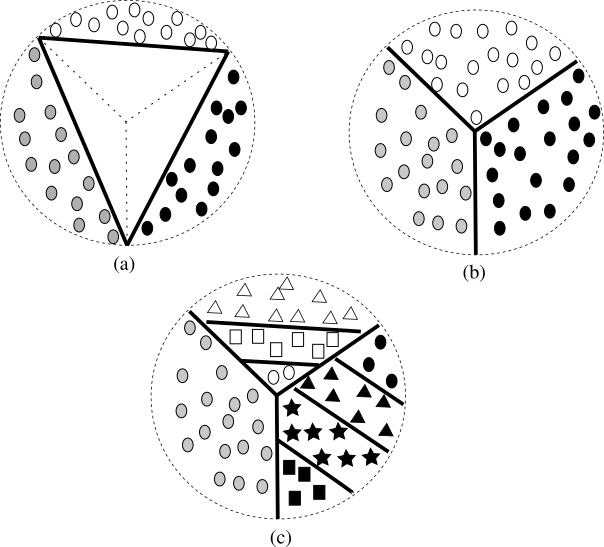
Figure 1: Three set of examples in ${\mathbb{R}}^{2}$ showing different linear separable conditions. Thick lines represent class boundaries. (a) Strongly linear separable examples with 3 classes (linearly separable in ${\mathbb{R}}^{3}$). (b) Weakly linear separable examples with 3 classes. (c) Group weakly linear separable examples with 3 groups; group 1 (white) contains 3 classes, group 2 (black) contains 4 classes, and group 3 (gray) contains 1 class.

2.2 Kernel methods

We give an overview of the kernel methods (see [7] for expositions) and the rational kernel [8].

The kernel method is a standard approach to extend linear classification algorithms that use only inner products to handle the notions of “distance” between pairs of examples to nonlinear classification. A positive definite kernel (or kernel) is a function of the form $k:X\times X\rightarrow{\mathbb{R}}$ for some set $X$ such that the matrix $[k(x_{i},x_{j})]_{i,j=1}^{m}$ is symmetric positive definite for any set of $m$ examples $x_{1},x_{2},\ldots,x_{m}\in X$. It is known that for every kernel $k$, there exists some inner product space $(V,\langle\cdot,\cdot\rangle)$ and a feature map $\phi:X\rightarrow V$ such that $k(x,x^{\prime})=\langle\phi(x),\phi(x^{\prime})\rangle$. Therefore, a linear learning algorithm can essentially non-linearly map every example into $V$ and work in $V$ instead of the original space without explicitly working with $\phi$ using $k$. This can be very helpful when the dimension of $V$ is infinite.

As in Beygelzimer et al. [1], we use the rational kernel. Assume that examples are in ${\mathbb{R}}^{d}$. Denote by ${\mathrm{B}}(0,1)$ a unit ball centered at $0$ in ${\mathbb{R}}^{d}$. The rational kernel $k:B(0,1)\times B(0,1)\rightarrow{\mathbb{R}}$ is defined as

$$k(x,x^{\prime})=\frac{1}{1-\frac{1}{2}\langle x,x^{\prime}\rangle_{{\mathbb{R}}^{d}}}.$$

Given $x,x^{\prime}\in{\mathbb{R}}^{d}$, $k(x,x^{\prime})$ can be computed in $O(d)$ time.

Let $\ell_{2}=\{x\in{\mathbb{R}}^{\infty}:\sum_{i=1}^{\infty}x_{i}^{2}<+\infty\}$ be the classical real separable Hilbert space equipped with the standard inner product $\langle x,x^{\prime}\rangle_{\ell_{2}}=\sum_{i=1}^{\infty}x_{i}x^{\prime}_{i}$. We can index the coordinates of $\ell_{2}$ by $d$-tuples $(\alpha_{1},\alpha_{2},\ldots,\alpha_{d})$ of non-negative integers, the associated feature map $\phi:{\mathrm{B}}(0,1)\rightarrow\ell_{2}$ to $k$ is defined as

$$\left(\phi(x_{1},x_{2},\ldots,x_{d})\right)_{(\alpha_{1},\alpha_{2},\ldots,\alpha_{d})}=x_{1}^{\alpha_{1}}x_{2}^{\alpha_{2}}\cdots x_{d}^{\alpha_{d}}\cdot\sqrt{2^{-(\alpha_{1}+\alpha_{2}+\cdots+\alpha_{d})}{{\alpha_{1}+\alpha_{2}+\cdots+\alpha_{d}}\choose{\alpha_{1},\alpha_{2},\ldots,\alpha_{d}}}},$$ (1)

where ${{\alpha_{1}+\alpha_{2}+\cdots+\alpha_{d}}\choose{\alpha_{1},\alpha_{2},\ldots,\alpha_{d}}}=\frac{(\alpha_{1}+\alpha_{2}+\cdots+\alpha_{d})!}{\alpha_{1}!\alpha_{2}!\cdots\alpha_{d}!}$ is the multinomial coefficient. It can be verified that $k$ is the kernel with its feature map $\phi$ to $\ell_{2}$ and for any $x\in{\mathrm{B}}(0,1)$, $\phi(x)\in\ell_{2}$.

2.3 Multiclass Linear Classification

Beygelzimer et al. [1] presented a learning algorithm for the strongly linearly separable examples using $K$ copies of the Binary Perceptron. They obtained a mistake bound of $O(K(R/\gamma)^{2})$ when the examples are from ${\mathbb{R}}^{d}$ with maximum norm $R$ with margin $\gamma$.

Their approach for dealing the weakly linear separable case is to use the kernel method. They introduced the Kernelized Bandit Algorithm (Algorithm 1) and proved the following theorem.

Data: Number of classes $K$, number of rounds $T$

Data: Kernel function $k(\cdot,\cdot)$

begin

       Initialize $J_{1}^{(1)}=J_{2}^{(2)}=\cdots=J_{k}^{(k)}=\emptyset$

       for $t=1,2,\ldots,T$ do

             Observe feature vector $x_{t}$

             Compute $S_{t}=\left\{i:1\leq i\leq K,\sum_{(x,y)\in J_{i}^{(t)}}yk(x,x_{t})\geq 0\right\}$

             if $S_{t}=\emptyset$ then

                   Predict $\hat{y}_{t}\sim\mbox{Uniform}(\{1,2,\ldots,K\})$

                   Observe feedback $z_{t}={\mathbbm{1}}[\hat{y}_{t}\neq y_{t}]$

                   if $z_{t}=1$ then

                         Set $J_{i}^{(t+1)}=J_{i}^{(t)}$ for all $i\in\{1,2,\ldots,K\}$

                  else

                         Set $J_{i}^{(t+1)}=J_{i}^{(t)}$ for all $i\in\{1,2,\ldots,K\}\setminus\{\hat{y}_{t}\}$

                         Update $J_{\hat{y}_{t}}^{(t+1)}=J_{\hat{y}_{t}}^{(t)}\cup\{(x_{t},+1)\}$

                   end if

                  

            else

                   Predict $\hat{y}_{t}\in S_{t}$ chosen arbitrarily

                   Observe feedback $z_{t}={\mathbbm{1}}[\hat{y}_{t}\neq y_{t}]$

                   if $z_{t}=1$ then

                         Set $J_{i}^{(t+1)}=J_{i}^{(t)}$ for all $i\in\{1,2,\ldots,K\}\setminus\{\hat{y}_{t}\}$

                         Update $J_{\hat{y}_{t}}^{(t+1)}=J_{\hat{y}_{t}}^{(t)}\cup\{(x_{t},-1)\}$

                  else

                         Set $J_{i}^{(t+1)}=J_{i}^{(t)}$ for all $i\in\{1,2,\ldots,K\}$

                   end if

                  

             end if

            

       end for

      

end

Algorithm 1 Kernelized Bandit Algorithm [1]

Theorem 1 (Theorem 4 from [1]).

Let $X$ be a non-empty set, let $(V,\langle\cdot,\cdot\rangle)$ be an inner product space. Let $\phi:X\rightarrow V$ be a feature map and let $k:X\times X\rightarrow{\mathbb{R}}$, where $k(x,x^{\prime})=\langle\phi(x),\phi(x^{\prime})\rangle$, be the kernel. If $(x_{1},y_{1}),(x_{2},y_{2}),\ldots,(x_{T},y_{T})\in X\times\{1,2,\ldots,K\}$ are labeled examples such that

1. the mapped examples $(\phi(x_{1}),y_{1}),\ldots,(\phi(x_{T}),y_{T})$ are strongly linearly separable with margin $\gamma$,

2. $k(x_{1},x_{1}),k(x_{2},x_{2}),\ldots,k(x_{T},x_{T})\leq R^{2}$

then the expected number of mistakes that the Kernelized Bandit Algorithm makes is at most $(K-1)\lfloor 4(R/\gamma)^{2}\rfloor$.

The key theorem for establishing the mistake bound is the following margin transformation theorem based on the rational kernel.

Theorem 2 (Theorem 5 from [1]).

(Margin transformation from [1]). Let $(x_{1},y_{1}),(x_{2},y_{2}),\ldots,(x_{T},y_{T})\in{\mathrm{B}}(0,1)\times[K]$ be a sequence of labeled examples that is weakly linear separable with margin $\gamma>0$. Let $\phi$ defined as in (1) let

$$\gamma_{1}=\frac{\left[376\lceil\log_{2}(2K-2)\rceil\cdot\left\lceil\sqrt{\frac{2}{\gamma}}\right\rceil\right]^{\frac{-\lceil\log_{2}(2K-2)\rceil\cdot\left\lceil\sqrt{2/\gamma}\right\rceil}{2}}}{2\sqrt{K}},$$

$$\gamma_{2}=\frac{\left(2^{s+1}r(K-1)(4s+2)\right)^{-(s+1/2)r(K-1)}}{4\sqrt{K}(4K-5)2^{K-1}}$$

where $r=2\lceil\frac{1}{4}\log_{2}(4K-3)\rceil+1$ and $s=\lceil\log_{2}(2/\gamma)\rceil$. Then the feature map $\phi$ makes the sequence $(\phi(x_{1}),y_{1}),(\phi(x_{2}),y_{2}),\ldots,(\phi(x_{T}),y_{T})$ strongly linearly separable with margin $\gamma^{\prime}=\max\{\gamma_{1},\gamma_{2}\}$. Also for all $t$, $k(x_{t},x_{t})\leq 2$.

This implies the following mistake bound.

Corollary 1 (Corollary 6 from [1]).

(Mistake upper bound from [1]). The mistake bound made by Algorithm 1 when the examples are weakly linearly separable with margin $\gamma$ is at most $\min(2^{\tilde{O}(K\log^{2}(1/\gamma))},2^{\tilde{O}(\sqrt{1/\gamma}\log K)})$.

Beygelzimer et al. [1] gave two margin transformation proofs. In this paper, we only provide one margin transformation based on the Chebyshev polynomials (Theorem 7 from [1]).

2.4 Our contribution

We consider labeled examples with group weakly linearly separable with margin $\gamma$ and show that in this case, the rational kernel also transforms the margin and the new margin depends on the number of groups $L$ instead of the number of classes $K$. More specifically we prove the margin transformation in Theorem 3 and show the mistake bound of $K\cdot 2^{\tilde{O}(\sqrt{1/\gamma}\log L)}$ in Corollary 2. This can be compared to one of the mistake bound of $K\cdot 2^{\tilde{O}(\sqrt{1/\gamma}\log K)}$ in [1].

The proofs are fairly technical. We follow the idea in [1] and construct a “good” polynomial that separates examples from one class to the other (strong separation) based on the Chebyshev polynomials [9].

3 Main result

Our main technical result is the following margin transformation using the rational kernel.

Theorem 3.

(Margin transformation). Let $(x_{1},y_{1}),(x_{2},y_{2}),\ldots,(x_{T},y_{T})\in{\mathrm{B}}(0,1)\times[K]$ be a sequence of labeled examples that is group weakly linear separable with margin $\gamma>0$. Let $L$ be number of group weakly separable such that $L\leq K.$ Let $\phi$ defined as in (1) let

$$\gamma^{\prime}=\frac{\left[840\lceil\log_{2}(2L+2)\rceil\cdot\left\lceil\sqrt{\frac{2}{\gamma}}\right\rceil\right]^{-\frac{\lceil\log_{2}(2L+2)\rceil\cdot\left\lceil\sqrt{\frac{2}{\gamma}}\right\rceil}{2}}}{9\sqrt{L}},$$

The feature map $\phi$ makes the sequence $(\phi(x_{1}),y_{1}),(\phi(x_{2}),y_{2}),\ldots,(\phi(x_{T}),y_{T})$ strongly linearly separable with margin $\gamma^{\prime}$.

We note that the margin depends on $L$, the number of groups, instead of $K$, the number of classes. Using Theorem 3 with Theorem 1 from [1] we obtain the following mistake bound for our algorithm.

Corollary 2.

(Mistake bound for group weakly linearly separable case) Let $K$ be positive integer, $L\leq K$ and $\gamma$ be positive real number. The mistake bound made by Algorithm 1 when the examples are group weakly linearly separable with margin $\gamma$ with $L$ groups is at most $K\cdot 2^{\tilde{O}(\sqrt{1/\gamma}\log L)}$.

Note that multiplicative factor of $K$ is hidden from the second bound of [1] because of the $\tilde{O}$ notation on the exponent. We cannot do that because in our exponent we have only $\log L$ which can be much smaller than $K$. Their actual bound (showing $K$), which can be compared to ours, is $K\cdot 2^{\tilde{O}(\sqrt{1/\gamma}\log K)}$.

3.1 Intra-group boundaries

We first prove a structural property of intra-group classes. The following lemma shows that it is possible to separate one class from the rest in the same group using only lower and upper thresholds. This is independent of the number of classes in that group.

Lemma 1.

For any group $i\in[L]$, for any class $y\in G_{i}$, there exists reals $b_{i}\leq t_{i}$ such that for all $t\in[T]$ such that (1) when $y_{t}=y$,

$$b_{i}+\gamma\leq\langle u^{\prime}_{i},x_{t}\rangle\leq t_{i}-\gamma;$$

and (2) when $g(y_{t})=g(y)$ but $y_{t}\neq y$, either

$$\langle x_{t},u^{\prime}_{i}\rangle\leq b_{i}-\gamma,$$

or

$$\langle x_{t},u^{\prime}_{i}\rangle\geq t_{i}+\gamma.$$

Proof.

Let $S_{y}=\{(x_{j},y_{j}):y_{j}=y,1\leq j\leq T\}$ be the set of examples with label $y$. Let $b_{i}=\min_{(x,y)\in S_{y}}\langle x,u^{\prime}_{i}\rangle-\gamma$ and $t_{i}=\max_{(x,y)\in S_{y}}\langle x,u^{\prime}_{i}\rangle+\gamma$. The lemma follows from the definition of group weakly linear separability. ∎

3.2 Margin transformation

This section is devoted to the proof of Theorem 3. A key property of the space $\ell_{2}$ is that it “contains” all multivariate polynomials and the rational kernel $k$ allows us to work in that space. More specifically, by (implicitly) transforming examples to $\ell_{2}$, we can use multivariate polynomials to separate examples from different classes, turning group weakly separability into strong linear separability in $\ell_{2}$. Therefore, to prove the margin transformation, as in [1], we have to (1) establish a separating polynomial and (2) prove the margin bound which depends on the degree and the norm of the polynomials (defined below).

Consider a $d$-variate polynomial $p:{\mathbb{R}}^{d}\rightarrow{\mathbb{R}}$ of the form

$$p(x)=p(x_{1},x_{2},\ldots,x_{d})=\sum_{\alpha_{1},\alpha_{2},\ldots,\alpha_{d}}c_{\alpha_{1},\alpha_{2},\ldots,\alpha_{d}}x_{1}^{\alpha_{1}}x_{2}^{\alpha_{2}}\cdots x_{d}^{\alpha_{d}},$$

where the sum ranges over a finite set of $d$-tuple $(\alpha_{1},\alpha_{2},\ldots,\alpha_{d})$ of non-negative integers and $c_{\alpha_{1},\alpha_{2},\ldots,\alpha_{d}}$’s are real coefficients. We denote the degree of $p$ as $deg(p)$. Following [4], the norm of a polynomial $p$ is defined as

$$\|p\|=\sqrt{\sum_{\alpha_{1},\alpha_{2},\ldots,\alpha_{d}}\left(c_{\alpha_{1},\alpha_{2},\ldots,\alpha_{d}}\right)^{2}}.$$

The following lemma from [1] expresses this intuition precisely.

Lemma 2 (from Lemma 9 in [1]).

(Norm bound) Let $p:{\mathbb{R}}^{d}\to{\mathbb{R}}$ be a multivariate polynomial. There exists $c\in\ell_{2}$ such that $p(x)=\langle c,\phi(x)\rangle_{\ell_{2}}$ and $\|c\|_{\ell_{2}}\leq 2^{deg(p)/2}\|p\|.$

As discussed previously, to prove Theorem 3, we need to show the existence of multivariate polynomials that separate one class from the other. Consider class $i\in[K]$ in group $g(i)$. Its positive example $x$, when compared with examples from other group $j\neq g(i)$, satisfies

$$\langle u_{g(i)},x\rangle-\langle u_{j},x\rangle=\langle u_{g(i)}-u_{j},x\rangle\geq\gamma,$$

implying that all examples in class $i$ lie in

$$R^{+}_{i}=\bigcap_{j\neq g(i)}\{x:\langle u_{g(i)}-u_{j},x\rangle\geq\gamma\},$$

while all examples in other groups lie in

$$R^{-}_{i}=\bigcup_{j\neq g(i)}\{x:\langle u_{g(i)}-u_{j},x\rangle\leq-\gamma\}.$$

When comparing with other classes $j$ in the same group $g(i)$, from Lemma 1, we know that there exists thresholds $b_{i}$ and $t_{i}$ that can be used to separate examples from group $i$, i.e., all its positive examples lie in

$$\hat{R}^{+}_{i}=\{x:\langle u^{\prime}_{g(i)},x\rangle\geq b_{i}+\gamma\}\cap\{x:\langle u^{\prime}_{g(i)},x\rangle\leq t_{i}-\gamma\},$$

while examples from other classes in group $g(i)$ lie in

$$\hat{R}^{-}_{i}=\{x:\langle u^{\prime}_{g(i)},x\rangle\leq b_{i}-\gamma\}\cup\{x:\langle u^{\prime}_{g(i)},x\rangle\geq t_{i}+\gamma\}.$$

Let $v_{b}=\frac{b_{i}}{\|u^{\prime}_{g(i)}\|}u^{\prime}_{g(i)}$ and $v_{t}=\frac{t_{i}}{\|u^{\prime}_{g(i)}\|}u^{\prime}_{g(i)}$. Both sets can be expressed as

$$\hat{R}^{+}_{i}= \ \{x:\langle u^{\prime}_{g(i)},x\rangle\geq\langle u^{\prime}_{g(i)},v_{b}\rangle+\gamma\}\ \cap\{x:\langle u^{\prime}_{g(i)},x\rangle\leq\langle u^{\prime}_{g(i)},v_{t}\rangle-\gamma\},$$

while examples from other classes in group $g(i)$ lie in

$$\hat{R}^{-}_{i}= \ \{x:\langle u^{\prime}_{g(i)},x\rangle\leq\langle u^{\prime}_{g(i)},v_{b}\rangle-\gamma\}\ \cup\{x:\langle u^{\prime}_{g(i)},x\rangle\geq\langle u^{\prime}_{g(i)},v_{t}\rangle+\gamma\}.$$

From Lemma 2, for class $i$, it is enough to establish a multivariate polynomial $p_{i}$ such that

$$x\in R^{+}_{i}\cap\hat{R}^{+}_{i} \ \ \ \Rightarrow p_{i}(x) \geq\gamma^{\prime}/2,$$

$$x\in R^{-}_{i}\cup\hat{R}^{-}_{i} \ \ \ \Rightarrow p_{i}(x) \leq-\gamma^{\prime}/2.$$

This is shown in Theorem 4 below. This theorem is fairly technical and is proved in Section 3.3.

Theorem 4.

(Polynomial approximation of intersection of halfspaces) Let $v_{1},v_{2},\ldots,v_{m}\in V$ such that $\|v_{1}\|,\|v_{2}\|,\ldots,\|v_{m}\|\leq 1$. Let $v_{b},v_{t}\in V$ such that $\|v_{b}\|\leq 1$ and $\|v_{t}\|\leq 1$. Let $v^{\prime}\in V$ such that $\|v^{\prime}\|\leq 1$. Let $\gamma\in(0,1)$ and $x\in{\mathrm{B}}(0,1)$. There exists a multivariate polynomial $p:{\mathbb{R}}^{d}\to{\mathbb{R}}$ such that

1. $p(x)\geq\frac{1}{2}$ for all $x\in\left(\bigcap_{i=1}^{m}\left\{x:\langle v_{i},x\rangle\geq\gamma\right\}\right)\cap\left\{x:\langle x,v^{\prime}\rangle\geq\langle v_{b},v^{\prime}\rangle+\gamma\right\}\cap\left\{x:\langle x,v^{\prime}\rangle\leq\langle v_{t},v^{\prime}\rangle-\gamma\right\},$

2. $p(x)\leq-\frac{1}{2}$ for all $x\in\left(\bigcup_{i=1}^{m}\left\{x:\langle v_{i},x\rangle\leq-\gamma\right\}\right)\cup\left\{x:\langle x,v^{\prime}\rangle\leq\langle v_{b},v^{\prime}\rangle-\gamma\right\}\cup\left\{x:\langle x,v^{\prime}\rangle\geq\langle v_{t},v^{\prime}\rangle+\gamma\right\},$

3. $deg(p)=\lceil\log_{2}(2m+4)\rceil\cdot\left\lceil\sqrt{\frac{2}{\gamma}}\right\rceil,$

4. $\|p\|\leq\frac{9}{2}\left[420\lceil\log_{2}(2m+4)\rceil\cdot\left\lceil\sqrt{\frac{2}{\gamma}}\right\rceil\right]^{\frac{\lceil\log_{2}(2m+4)\rceil\cdot\left\lceil\sqrt{\frac{2}{\gamma}}\right\rceil}{2}}$

Proof of Theorem 3.

Consider class $i\in[K]$. We will apply Theorem 4. For $j\in\{1,\ldots,L-1\}$, let

$$v_{j}=\left\{\begin{array}[]{ll}u_{g(i)}-u_{j},&\mbox{if $j<g(i)$,}\\ u_{g(i)}-u_{j+1},&\mbox{if $j>g(i)$.}\end{array}\right.$$

Also, let $v^{\prime}=u^{\prime}_{g(i)}$, $v_{b}=\frac{b_{i}}{\|u^{\prime}_{g(i)}\|}u^{\prime}_{g(i)}$ and $v_{t}=\frac{t_{i}}{\|u^{\prime}_{g(i)}\|}u^{\prime}_{g(i)}$.

From Theorem 4, there exists a multivariate polynomial $p_{i}:{\mathbb{R}}^{d}\to{\mathbb{R}}$ such that for all $t\in[T]$ and the sequence $(x_{1},y_{1}),(x_{2},y_{2}),(x_{t},y_{t}),\ldots,(x_{T},y_{T})$, we have

• if $y_{t}=i$, $p_{i}(x_{t})\geq\frac{1}{2}$, since $x_{t}\in R^{+}_{i}\cap\hat{R}^{+}_{i}$, and

• if $y_{t}\neq i,$ $p_{i}(x_{t})\leq-\frac{1}{2}$, since $x_{t}\in R^{-}_{i}\cap\hat{R}^{-}_{i}$.

It is left to check the properties of $p$. Theorem 4 implies that

$$\|p\|\leq\frac{9}{2}\left[420\lceil\log_{2}(2L+2)\rceil\cdot\left\lceil\sqrt{\frac{2}{\gamma}}\right\rceil\right]^{\frac{\lceil\log_{2}(2L+2)\rceil\cdot\left\lceil\sqrt{\frac{2}{\gamma}}\right\rceil}{2}}$$

By Lemma 2, there exists $c_{i}\in\ell_{2}$ such that $\langle c_{i},\phi(x)\rangle=p_{i}(x),$ and

$$\|c_{i}\|_{\ell_{2}}\leq\frac{9}{2}\left[840\lceil\log_{2}(2L+2)\rceil\cdot\left\lceil\sqrt{\frac{2}{\gamma}}\right\rceil\right]^{\frac{\lceil\log_{2}(2L+2)\rceil\cdot\left\lceil\sqrt{\frac{2}{\gamma}}\right\rceil}{2}}.$$

We are ready to construct strongly separable vectors for our group weakly separable case in $\ell_{2}$ such that $\|z_{1}\|^{2}+\|z_{2}\|^{2}+\ldots+\|z_{L}\|^{2}\leq 1$ and for all $t\in[T]$, $\langle z_{y_{t}},x_{t}\rangle\geq\gamma$, and for all $j\neq y_{t}$, $\langle z_{j},x_{t}\rangle\leq-\gamma$, by scaling $c_{i}$ appropriately as follows. We can let

$$z_{i}=\frac{c_{i}}{\sqrt{L}\cdot\frac{9}{2}\left[840\lceil\log_{2}(2L+2)\rceil\cdot\left\lceil\sqrt{\frac{2}{\gamma}}\right\rceil\right]^{\frac{\lceil\log_{2}(2L+2)\rceil\cdot\left\lceil\sqrt{\frac{2}{\gamma}}\right\rceil}{2}}},$$

and

$$\gamma=\frac{\left[840\lceil\log_{2}(2L+2)\rceil\cdot\left\lceil\sqrt{\frac{2}{\gamma}}\right\rceil\right]^{-\frac{\lceil\log_{2}(2L+2)\rceil\cdot\left\lceil\sqrt{\frac{2}{\gamma}}\right\rceil}{2}}}{9\sqrt{L}},$$

then the theorem follows. ∎

3.3 Separating polynomials

This section proves Theorem 4, i.e., we provide a polynomial $p:{\mathbb{R}}^{d}\rightarrow{\mathbb{R}}$ that separates one class of examples from the others with degree and norm bounds.

As in [1] and [4], we use the Chebyshev polynomials [9] $T_{n}(\cdot)$ defined as follows.

$$T_{0}(z) =1,$$

$$T_{1}(z) =z,$$

$$T_{n+1} =2zT_{n}(z)-T_{n-1}(z)\;\;\text{for $n\geq 1$}$$

The following two lemmas are from [1].

Lemma 3 (from Lemma 15 in [1]).

(Properties of Chebyshev polynomials) Chebyshev polynomials satisfy

1. $deg(T_{n})=n$ for all $n\geq 0$.

2. If $n\geq 1$, the leading coefficient of $T_{n}(z)$ is $2^{n-1}$.

3. $T_{n}(\cos(\theta))=\cos(n\theta)$ for all $\theta\in{\mathbb{R}}$ and all $n\geq 0$.

4. $T_{n}(\cosh(\theta))=\cosh(n\theta)$ for all $\theta\in{\mathbb{R}}$ and all $n\geq 0$.

5. $|T_{n}(z)|\leq 1$ for all $z\in[-1,1]$ and all $n\geq 0$.

6. $T_{n}(z)\geq 1+n^{2}(z-1)$ for all $z\geq 1$ and all $n\geq 0$.

7. $\|T_{n}\|\leq(1+\sqrt{2})^{n}$ for all $n\geq 0$.

Lemma 4 (from Lemma 14 in [1]).

(Properties of norm of polynomials)

1. Let $p_{1},p_{2},\ldots,p_{n}$ be multivariate polynomials and let $p(x)=\prod_{j=1}^{n}p_{j}(x)$ be their product. Then, $\|p\|^{2}\leq n^{\sum_{j=1}^{n}deg(p_{j})}\prod_{j=1}^{n}\|p_{j}\|^{2}$.

2. Let $q$ be a multivariate polynomial of degree at most $s$ and let $p(x)=(q(x))^{n}$. Then, $\|p\|^{2}\leq n^{ns}\|q\|^{2n}$.

3. Let $p_{1},p_{2},\ldots,p_{n}$ be multivariate polynomials. Then, $\left\|\sum_{j=1}^{n}p_{j}\right\|^{2}\leq n\sum_{j=1}^{n}\|p_{j}\|^{2}.$

Our proof follows the approach in [1].

Proof of Theorem 4.

Let $r=\lceil\log_{2}(2m+4)\rceil$ and $s=\left\lceil\sqrt{\frac{2}{\gamma}}\right\rceil$. Define the polynomial $p:{\mathbb{R}}^{d}\to{\mathbb{R}}$ as

$$p(x) =m+\frac{5}{2}-\sum_{i=1}^{m}(T_{s}(1-\langle v_{i},x\rangle))^{r}-(T_{s}(1-\langle x-v_{b},v^{\prime}\rangle/2))^{r}-(T_{s}(1-\langle v_{t}-x,v^{\prime}\rangle/2))^{r}.$$

First, consider the case when

$$x\in \left(\bigcap_{i=1}^{m}\left\{x:\langle v_{i},x\rangle\geq\gamma\right\}\right)\cap\left\{x:\langle x,v^{\prime}\rangle\geq\langle v_{b},v^{\prime}\rangle+\gamma\right\}\cap\left\{x:\langle x,v^{\prime}\rangle\leq\langle v_{t},v^{\prime}\rangle-\gamma\right\}.$$

Note that $\langle v_{i},x\rangle\geq\gamma$ for all $i\in[m]$. Since $\|x\|\leq 1$ and $\|v_{i}\|\leq 1$, we have $\langle v_{i},x\rangle\in[0,1]$; thus, $(T_{s}(1-\langle v_{i},x\rangle))^{r}\in[-1,1]$. Consider the terms involving $v_{b}$ and $v_{t}$. Since $\|x\|,\|v_{b}\|,\|v_{t}\|\leq 1$, we have that $\|x-v_{b}\|\leq 2$ and $\|v_{t}-x\|\leq 2$. This implies that $1\geq\langle x-v_{b},v^{\prime}\rangle/2\geq\gamma/2$ and $1\geq\langle v_{t}-x,v^{\prime}\rangle/2\geq\gamma/2$; hence, $(T_{s}(1-\langle x-v_{b},v^{\prime}\rangle/2))^{r}\in[-1,1]$ and $(T_{s}(1-\langle v_{t}-x,v^{\prime}\rangle/2))^{r}\in[-1,1]$. Therefore,

$$p(x)\geq m+\frac{5}{2}-m-1-1\geq\frac{1}{2}.$$

Now consider the case when

$$x\in \bigcup_{i=1}^{m}\left\{x:\langle v_{i},x\rangle\leq-\gamma\right\}\cup\left\{x:\langle x,v^{\prime}\rangle\leq\langle v_{b},v^{\prime}\rangle-\gamma\right\}\cup\left\{x:\langle x,v^{\prime}\rangle\geq\langle v_{t},v^{\prime}\rangle+\gamma\right\}$$

There are two subcases to consider.

Subcase 1: Suppose that for some $i$, $\langle v_{i},x\rangle\leq-\gamma$. In this case, $1-\langle v_{i},x\rangle\geq 1+\gamma$ and Lemma 3 (part 6) implies that

$$T_{s}(1-\langle v_{i},x\rangle)\geq 1+s^{2}\gamma\geq 1+2\geq 2,$$

and thus, $(T_{s}(1-\langle v_{i},x\rangle))^{r}\geq 2^{r}\geq 2m+4$.

Since $T_{s}(1-\langle v_{i},x\rangle))^{r}\geq-1$ for all $i$, $(T_{s}(1-\langle x-v_{b},v^{\prime}\rangle/2))^{r}\geq-1$, and $(T_{s}(1-\langle v_{t}-x,v^{\prime}\rangle/2))^{r}\geq-1$, we have that

$$p(x) =m+\frac{5}{2}-(T_{s}(1-\langle v_{i},x\rangle))^{r}-\sum_{j\in[m]j\neq i}(T_{s}(1-\langle v_{j},x\rangle))^{r}$$

$$\;\;\;\;\;-(T_{s}(1-\langle x-v_{b},v^{\prime}\rangle/2))^{r}-(T_{s}(1-\langle v_{t}-x,v^{\prime}\rangle/2))^{r}$$

$$\leq m+\frac{5}{2}-(2m+4)+(m-1)+2\leq-\frac{1}{2}.$$

Subcase 2: Consider the other case when for all $i$, $\langle v_{i},x\rangle>-\gamma$. We deal with the case that $\langle x,v^{\prime}\rangle\leq\langle v_{b},v^{\prime}\rangle-\gamma$. The case when $\langle x,v^{\prime}\rangle\geq\langle v_{t},v^{\prime}\rangle+\gamma$ can be handled similarly.

Since $\langle x-v_{b},v^{\prime}\rangle\leq-\gamma$, we have $1-\langle x-v_{b},v^{\prime}\rangle/2\geq 1+\gamma/2$. Lemma 3 (part 6) implies that

$$T_{s}(1-\langle x-v_{b},v^{\prime}\rangle/2)\geq 1+s^{2}\gamma/2\geq 1+2/2\geq 2,$$

and $(T_{s}(1-\langle x-v_{b},v^{\prime}\rangle/2))^{r}\geq 2m+4$. Applying the same argument as in Subcase 1, this implies that $p(x)\leq-\frac{1}{2}$.

The degree of $p$ is the maximum degree of the terms $(T_{s}(1-\langle v_{i},x\rangle))^{r}$, $(T_{s}(1-\langle x-v_{b},v^{\prime}\rangle/2))^{r}$, and $(T_{s}(1-\langle v_{t}-x,v^{\prime}\rangle/2))^{r}$; thus, it is $r\cdot s$.

Finally, we prove the upper bound of norm of $p$. We first deal with the term $T_{s}(1-\langle v_{i},x\rangle)$.

Let $f_{i}(x)=1-\langle v_{i},x\rangle$ and $g_{i}(x)=T_{s}(1-\langle v_{i},x\rangle)=T_{s}(f_{i}(x))$. We have

$$\|f_{i}\|^{2}=1+\|v_{i}\|^{2}\leq 1+1=2.$$

Let $T_{s}(z)=\sum_{j=0}^{s}c_{j}z^{j}$ be the expansion of $s$-th Chebyshev polynomial. We can bound the term $\|g_{i}\|^{2}$ as follows.

$$\|g_{i}\|^{2} =\left\|\sum_{j=0}^{s}c_{j}(f_{i})^{j}\right\|^{2}$$

$$\leq(s+1)\sum_{j=0}^{s}\left\|c_{j}(f_{i})^{j}\right\|^{2}\qquad\qquad\qquad\mbox{(by part 3 of Lemma~{}\ref{lem:poly-prop})}$$

$$=(s+1)\sum_{j=0}^{s}c_{j}^{2}\left\|(f_{i})^{j}\right\|^{2}$$

$$\leq(s+1)\sum_{j=0}^{s}c_{j}^{2}j^{j}\left\|f_{i}\right\|^{2j}\qquad\qquad\qquad\mbox{(by part 2 of Lemma~{}\ref{lem:poly-prop})}$$

$$\leq(s+1)\sum_{j=0}^{s}c_{j}^{2}j^{j}2^{2j}$$

$$\leq(s+1)s^{s}2^{2s}\sum_{j=0}^{s}c_{j}^{2}$$

$$=(s+1)s^{s}2^{2s}\|T_{s}\|^{2}$$

$$=(s+1)s^{s}2^{2s}(1+\sqrt{2})^{2s}\qquad\qquad\qquad\mbox{(by part 7 of Lemma~{}\ref{lem:cheby-prop})}$$

$$=(s+1)\left(4(1+\sqrt{2})^{2}s\right)^{s}$$

$$\leq(8(1+\sqrt{2})^{2}s)^{s}\qquad\qquad\qquad\qquad\quad\mbox{(because $s+1\leq 2^{s}$)}$$

$$\leq(47s)^{s}.$$

We now deal with the terms $(T_{s}(1-\langle x-v_{b},v^{\prime}\rangle/2))^{r}$, and $(T_{s}(1-\langle v_{t}-x,v^{\prime}\rangle)/2)^{r}$.

Let $h_{b}(x)=1-\langle x-v_{b},v^{\prime}\rangle/2$ and $h_{t}(x)=1-\langle v_{t}-x,v^{\prime}\rangle/2$. Let $q_{b}(x)=T_{s}(1-\langle x-v_{b},v^{\prime}\rangle/2)=T_{s}(h_{b}(x))$ and $q_{t}(x)=T_{s}(1-\langle v_{t}-x,v^{\prime}\rangle/2)=T_{s}(h_{t}(x))$. We have

$$\|h_{b}\|^{2}\leq\left\|\frac{v^{\prime}}{2}\right\|^{2}+\left(1+\frac{\|v_{b}\|\|v^{\prime}\|}{2}\right)^{2}\leq\frac{1}{4}+\left(1+\frac{1}{2}\right)^{2}=\frac{10}{4}\leq 3,$$

and

$$\|h_{t}\|^{2}\leq\left\|\frac{v^{\prime}}{2}\right\|^{2}+\left(1+\frac{\|v_{t}\|\|v^{\prime}\|}{2}\right)^{2}\leq\frac{1}{4}+\left(1+\frac{1}{2}\right)^{2}=\frac{10}{4}\leq 3,$$

since $h_{b}(x)=\langle x,v^{\prime}/2\rangle+(1+\langle v_{b},v^{\prime}/2\rangle)$ and $h_{t}(x)=-\langle x,v^{\prime}/2\rangle+(1-\langle v_{t},v^{\prime}/2\rangle)$.

The terms $\|q_{b}\|^{2}$ and $\|q_{t}\|^{2}$ can be analyzed similarly as $\|g_{i}\|^{2}$. We have that

$$\|q_{b}\|^{2} =\left\|\sum_{j=0}^{s}c_{j}(h_{b})^{j}\right\|^{2}$$

$$\leq(s+1)\sum_{j=0}^{s}c_{j}^{2}j^{j}\left\|h_{b}\right\|^{2j}\qquad\qquad\qquad\mbox{(by parts 2 and 3 of Lemma~{}\ref{lem:poly-prop})}$$

$$\leq(s+1)\sum_{j=0}^{s}c_{j}^{2}j^{j}3^{2j}$$

$$\leq(s+1)s^{s}3^{2s}\sum_{j=0}^{s}c_{j}^{2}$$

$$=(s+1)s^{s}3^{2s}\|T_{s}\|^{2}$$

$$=(s+1)s^{s}3^{2s}(1+\sqrt{2})^{2s}\qquad\qquad\qquad\mbox{(by part 7 of Lemma~{}\ref{lem:cheby-prop})}$$

$$=(s+1)\left(9(1+\sqrt{2})^{2}s\right)^{s}$$

$$\leq(9(1+\sqrt{2})^{2}s)^{s}$$

$$\leq(105s)^{s}$$

and

$$\|q_{t}\|^{2} =\left\|\sum_{j=0}^{s}c_{j}(h_{t})^{j}\right\|^{2}$$

$$\leq(105s)^{s}.$$

Finally,

$$\|p\| \leq m+\frac{5}{2}+\sum_{i=1}^{m}\left\|(g_{i})^{r}\right\|+\left\|(q_{b})^{r}\right\|+\left\|(q_{t})^{r}\right\|$$

$$=m+\frac{5}{2}+\sum_{i=1}^{m}\sqrt{\left\|(g_{i})^{r}\right\|^{2}}+\sqrt{\left\|(q_{b})^{r}\right\|^{2}}+\sqrt{\left\|(q_{t})^{r}\right\|^{2}}$$

$$\leq m+\frac{5}{2}+\sum_{i=1}^{m}\sqrt{r^{rs}\left\|g_{i}\right\|^{2r}}+\sqrt{r^{rs}\left\|q_{b}\right\|^{2r}}+\sqrt{r^{rs}\left\|q_{t}\right\|^{2r}}$$

$$\leq m+\frac{5}{2}+mr^{rs/2}(47s)^{rs/2}+r^{rs/2}(105s)^{rs/2}+r^{rs/2}(105s)^{rs/2}$$

$$\leq m+\frac{5}{2}+(m+2)(105rs)^{rs/2}.$$

Using the fact that $m\leq\frac{1}{2}2^{r}$ and $r,s\geq 1$, we then have

$$\|p\| \leq m+\frac{5}{2}+(m+2)(105rs)^{rs/2}$$

$$\leq\frac{1}{2}2^{r}+\frac{5}{2}+\left(\frac{1}{2}2^{r}+2\right)(105rs)^{rs/2}$$

$$\leq 2\cdot 2^{r}+\frac{5}{2}\cdot 2^{r}(105rs)^{rs/2}$$

$$=2^{r}\left(2+\frac{5}{2}\right)(105rs)^{rs/2}$$

$$\leq 4^{rs/2}\cdot\frac{9}{2}(105rs)^{rs/2}$$

$$=\frac{9}{2}(420rs)^{rs/2}.$$

Substitutions of $r$ and $s$ finish the proof. ∎

4 Experiments

While we focus mostly on the theoretical aspect of the problem, we performed some experiment to visualize the algorithm.

We generated a dataset in ${\mathbb{R}}^{2}$ under the group weakly linear separable condition, with $K=9$ classes and $L=3$ groups with margin $\gamma=0.005$, shown in Fig 2.

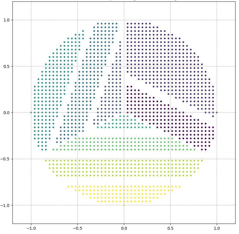
Figure 2: Group weakly separable dataset in ${\mathbb{R}}^{2}$.

We compared two versions of the bandit multiclass perceptron [1], the standard one and the kernelized one (using the rational kernel). Since the standard one only works with strongly separable case, it would definitely fail in this experiment, but we used it to give an overall sense of improvement for the kernelized version. We ran both algorithms for $T=10^{6}$ steps. For the kernelized version, we conducted 5 experiments, while the linear one we only ran once. Fig. 3 shows the result. The kernelized version made on average $130,884.6$ mistakes ($13.1\%$), while the standard one made $835,848$ mistakes ($83.6\%$). Theoretically, the kernelized version should stop making mistakes at some point, but since the number of steps that we ran is too low, we can only see that increasing rate of the number of mistakes decreases over time.

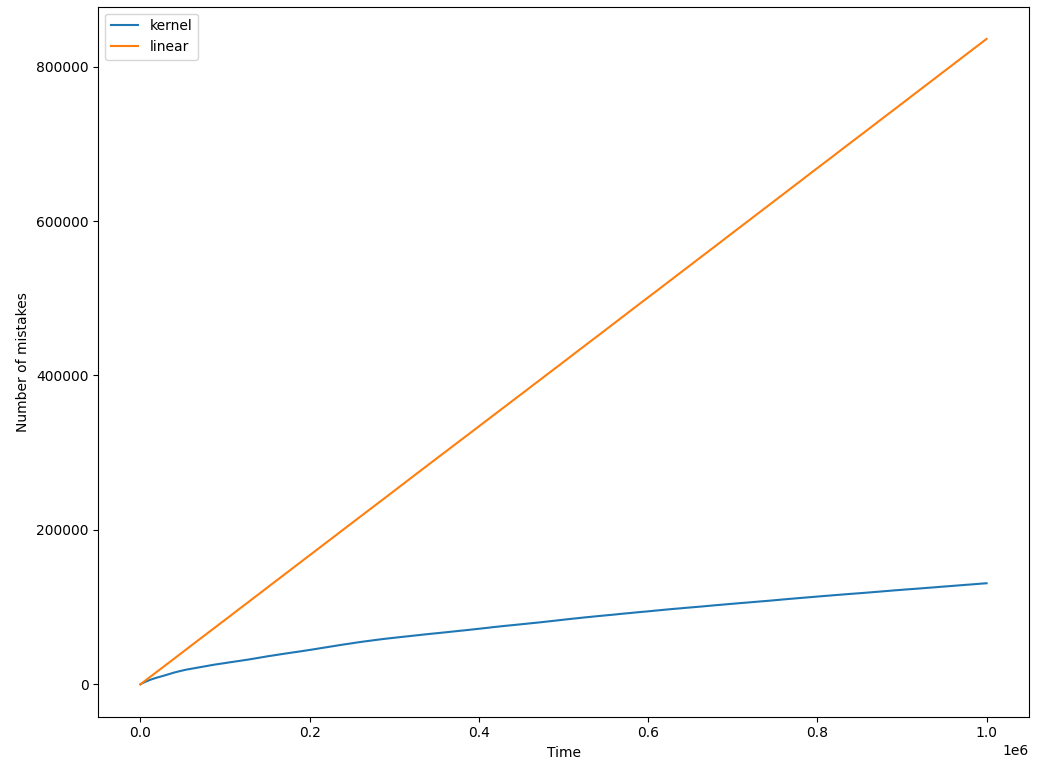
Figure 3: Comparison of the standard algorithm and the kernelized algorithm with $T=10^{6}$.

To see the decision boundary, we ploted the contours of the corresponding polynomials for two classes shown in Fig. 4 and Fig. 5. Note that the class in Fig. 5 was much harder to learn as its boundary still overlapped with other classes (i.e., mistakes could still be made).

Figure 4: The decision contours of a class (in black) of the kernelized algorithm after $T=10^{6}$ steps.

Figure 5: The decision contours of a class (in black) of the kernelized algorithm after $T=10^{6}$ steps.

5 Acknowledgements

We thank Sanparith Marukatat for insightful comments and for pointing out our calculation errors. We also thank Thanawin Rakthanmanon for useful comments.

Funding: Both authors are supported by the Thailand Research Fund, Grant RSA-6180074.

References

-
[1]
A. Beygelzimer, D. Pal, B. Szorenyi, D. Thiruvenkatachari, C.-Y. Wei, C. Zhang,
Bandit multiclass
linear classification: Efficient algorithms for the separable case, in:
K. Chaudhuri, R. Salakhutdinov (Eds.), Proceedings of the 36th International
Conference on Machine Learning, Vol. 97 of Proceedings of Machine Learning
Research, PMLR, Long Beach, California, USA, 2019, pp. 624–633.
URL http://proceedings.mlr.press/v97/beygelzimer19a.html - [2] K. Crammer, Y. Singer, Ultraconservative online algorithms for multiclass problems, J. Mach. Learn. Res. 3 (2003) 951–991. doi:10.1162/jmlr.2003.3.4-5.951.
- [3] S. M. Kakade, S. Shalev-Shwartz, A. Tewari, Efficient bandit algorithms for online multiclass prediction, in: Proceedings of the 25th International Conference on Machine Learning, ICML ’08, ACM, New York, NY, USA, 2008, pp. 440–447. doi:10.1145/1390156.1390212.
- [4] A. R. Klivans, R. A. Servedio, Learning intersections of halfspaces with a margin, Journal of Computer and System Sciences 74 (1) (2008) 35 – 48, learning Theory 2004. doi:https://doi.org/10.1016/j.jcss.2007.04.012.
- [5] R. Beigel, N. Reingold, D. Spielman, Pp is closed under intersection, Journal of Computer and System Sciences 50 (2) (1995) 191 – 202. doi:https://doi.org/10.1006/jcss.1995.1017.
- [6] G. Chen, G. Chen, J. Zhang, S. Chen, C. Zhang, Beyond banditron: A conservative and efficient reduction for online multiclass prediction with bandit setting model, in: ICDM 2009, The Ninth IEEE International Conference on Data Mining, Miami, Florida, USA, 6-9 December 2009, 2009, pp. 71–80. doi:10.1109/ICDM.2009.36.
- [7] J. Shawe-Taylor, N. Cristianini, Kernel Methods for Pattern Analysis, Cambridge University Press, New York, NY, USA, 2004.
-
[8]
S. Shalev-Shwartz, O. Shamir, K. Sridharan,
Learning kernel-based halfspaces
with the 0-1 loss, SIAM J. Comput. 40 (6) (2011) 1623–1646.
doi:10.1137/100806126.
URL https://doi.org/10.1137/100806126 - [9] J. Mason, D. Handscomb, Chebyshev Polynomials, CRC Press, 2002.