Using coupling methods to estimate sample quality for stochastic differential equations

Abstract.

A probabilistic approach for estimating sample qualities for stochastic differential equations is introduced in this paper. The aim is to provide a quantitative upper bound of the distance between the invariant probability measure of a stochastic differential equation and that of its numerical approximation. In order to extend estimates of finite time truncation error to infinite time, it is crucial to know the rate of contraction of the transition kernel of the SDE. We find that suitable numerical coupling methods can effectively estimate such rate of contraction, which gives the distance between two invariant probability measures. Our algorithms are tested with several low and high dimensional numerical examples.

1. Introduction

Stochastic differential equations (SDEs) are widely used in many scientific fields. Under mild assumptions, an SDE would admit a unique invariant probability measure, denoted by $\pi$. In many applications including but not limited to Markov chain Monte Carlo and molecular dynamics, it is important to sample from $\pi$ [1, 28]. This is usually done by either numerically integrating an SDE over a very long trajectories or integrating many trajectories of the SDE over a finite time [37]. However, a numerical integrator of the SDE typically has a different invariant probability measure, denoted by $\hat{\pi}$, that depends on the time discretization [43, 44, 41]. A natural question is that, how is $\hat{\pi}$ different from $\pi$? In other words, what is the quality of data sampled from a numerical trajectory of the SDE? This is very different from the classical truncation error analysis, which is only applicable for finite time intervals except some special cases [27, 10].

Theoretically, it is well known that the distance between $\pi$ and $\hat{\pi}$ can be controlled if we have good estimate of (i) the finite time truncation error and (ii) the rate of geometric ergodicity of the SDE. Estimates of this type can be made by various different approaches [34, 35, 8, 5, 6]. Roughly speaking, if the truncation error over a finite time interval $[0,T]$ is $O(\epsilon)$, and the rate of geometric ergodicity is $\gamma$ (i.e. speed of convergence to $\pi$ is $\approx\gamma^{t}$ for $\gamma\in(0,1)$), then the difference between $\pi$ and $\hat{\pi}$ is $O(\epsilon(1-\gamma^{T})^{-1})$. (See our discussion in Section 3.1 for details.) However, these approaches can not give a quantitative estimate in general, as the rate of geometric ergodicity $\gamma$ estimated by rigorous approaches are usually very far from being sharp. Many approaches such as the Lyapunov function method can only rigorously show that the speed of convergence is $\approx\gamma^{t}$ for some $\gamma<1$ [36, 16, 17]. Looking into the proof more carefully, one can easily find that this $\gamma$ has to be extremely close to $1$ to make the proof work. This gives a very large $(1-\gamma^{T})^{-1}$ and makes rigorous estimates difficult to use in practice. To the best of our knowledge, quantitative estimates of convergence rate can only be proved for a few special cases like stochastic gradient flow and Langevin dynamics [14, 7, 2].

The aim of this paper is to provide some algorithms to numerically estimate the distance between $\pi$ and $\hat{\pi}$. The finite time truncation error over a time interval $[0,T]$ is estimated by using extrapolations, which is a common practice in numerical analysis. The main novel part is the estimation of the rate of contraction of the transition kernel. Traditional approaches for computing the rate of geometric ergodicity are either computing principal eigenvalue of the discretized generator or estimating the decay rate of correlation. The eigenvalue method works well in low dimension but faces significant challenge if the SDE is in dimension $\geq 3$. The correlation decay is difficult to estimate as well, because a correlation has exponentially small expectation and large variance. One needs a huge amount of samples to estimate it effectively. In addition, exponential decay of correlation with respect to an ad-hoc observable is usually not very convincing. In this paper, we propose to estimate the rate of contraction of the transition kernel by using a coupling technique.

Coupling methods have been used in rigorous proofs for decades [31, 32, 13, 39]. The idea is to run two trajectories of a random process $X_{t}$, such that one is from a given initial distribution and the other is stationary. A suitable joint distribution, called a coupling, is constructed in the product space, such that two marginals of this joint process are the original two trajectories. If after some time, the two processes stay together with high probability, then the law of $X_{t}$ must be very close to its invariant probability measure. It is well known that the coupling lemma gives bounds of both total variation norm and some 1-Wasserstein-type distances. In this paper, we use the coupling method numerically. If two numerical trajectories meet each other, they are coupled and evolve together after coupling. By the coupling lemma, the contraction rate of the transition kernel can be estimated numerically by computing the probability of successful coupling, which follows from running a Monte Carlo simulation. Together with the finite time error, we can estimate the distance between $\pi$ and $\hat{\pi}$. The main advantage of coupling method is that it is relatively dimension-free, and we demonstrate our technique on an SDE system in $\mathbb{R}^{80}$ in Section 4.5.

We provide two sets of algorithms, one for a quantitative upper bound and the other for a rough but quick estimate. To get the quantitative upper bound, one needs an upper bound of the contraction rate of 1-Wasserstein distance for all pairs of initial values starting from a certain compact set $\Omega\times\Omega$. This is done by applying extreme value theory. More precisely, we uniformly sample initial values from $\Omega\times\Omega$ and compute the contraction rate by using the coupling method. Then the upper bound of such contraction rate can be obtained by numerically fitting a generalized Pareto distribution (GPD) [9, 3]. In practice, one may want a low cost estimate for the quality of samples. Hence we provide a “rough estimate” that only uses the exponential tail of the coupling probability as the rate of contraction of the generator after a given time $T$. This rough estimate differs from the true upper bound by an unknown constant, but it is more efficient and works well empirically.

Our coupling method can be applied to SDEs with degenerate random terms after suitable modifications. This is done by comparing the overlap of the probability density functions after two or more steps of the numerical scheme. Our approach is demonstrated on a Langevin dynamics example in Section 4.3. It is known from [14, 7] that a suitable mixture of reflection coupling and synchronous coupling can be used for Langevin equation. We find that this approach can be successfully combined with the “maximal coupling” for the numerical scheme. However, for SDEs with very degenerate noise, using the coupling method remains to be a great challenge.

We test our algorithm with a few different examples, from simple to complicated. The sharpness of our algorithm is checked by using a “ring density example” whose invariant probability density function can be explicitly given. Then we demonstrate the use of coupling method under degenerate noise by working with a 4D Langevin equation. Next we show two examples whose numerical invariant probability differs $\hat{\pi}$ significantly from true invariant probability measure $\pi$. One is an asymmetric double well potential whose transition kernel has a slow rate of convergence. The other example is the Lorenz 96 model whose finite time truncation error is very difficult to control due to intensive chaos. Finally, we study a coupled FizHugh-Nagumo oscillator model proposed in [11, 24] to demonstrate that our algorithm works reasonably well in high dimensional problems.

The organization of this paper is as follows. Section 2 serves as the probability preliminary, in which we review some necessary background about the coupling method, stochastic differential equations, and numerical SDE schemes. The main algorithm is developed in Section 3. All numerical examples are demonstrated in Section 4. Section 5 is the conclusion.

2. Probability preliminary

In this section, we provide some necessary probability preliminaries for this paper, which are about the coupling method, stochastic differential equations, numerical stochastic differential equations, and convergence analysis.

2.1. Coupling

This subsection provides the definition of coupling of random variables and Markov processes.

Definition 2.1 (Coupling of probability measures).

Let $\mathbb{P}$ and $\mathbb{P}^{\prime}$ be two probability measures on a probability space $(\Omega,\mathcal{F})$. A probability measure $\gamma$ on $(\Omega\times\Omega,\mathcal{F}\times\mathcal{F})$ is called a coupling of $\mathbb{P}$ and $\mathbb{P}^{\prime}$, if two marginals of $\gamma$ coincide with $\mathbb{P}$ and $\mathbb{P}^{\prime}$ respectively.

The definition of coupling can be extended to any two random variables that take value in the same state space.

Definition 2.2 (Markov Coupling).

A Markov coupling of two Markov processes $X_{t}$ and $Y_{t}$ with transition kernel $P$ is a Markov process $(\tilde{X}_{t},\tilde{Y}_{t})$ on the product state space $V\times V$ such that

• The marginal processes $X_{t}$ and $Y_{t}$ are Markov processes with transition kernel $P$, and

• If $\tilde{X}_{s}=\tilde{Y}_{s}$, we have $\tilde{X}_{t}=\tilde{Y}_{t}$ for all $t>s$.

Markov coupling can be defined in many different ways. For example, let $P$ be the transition kernel of a Markov chain $X_{t}$ on a countable state space $V$, the following transition kernel $Q$ for $(\tilde{X}_{t},\tilde{Y}_{t})$ on $V\times V$ such that

$$Q^{t}((x_{1},y_{1}),(x_{2},y_{2}))=\left\{\begin{array}[]{ll}P^{t}(x_{1},x_{2})P^{t}(y_{1},y_{2}),&\text{if }x_{1}\neq y_{1}\\ P^{t}(x_{1},x_{2}),&\text{if }x_{1}=y_{1}\text{ and }x_{2}=y_{2}\\ 0,&\text{if }x_{1}=y_{1}\text{ and }x_{2}\neq y_{2}\end{array}\right.,$$

is called the independent coupling. Paths of the two marginal processes are independent until they first meet. In the rest of this paper, unless otherwise specified, we only consider Markov couplings.

2.2. Wasserstein distance and total variation distance

In order to give an estimate for the coupling of Markov processes, we need the following to metrics.

Definition 2.3 (Wasserstein distance).

Let $d$ be a metric on the state space $V$. For probability measures $\mu$ and $\nu$ on $V$, the Wasserstein distance between $\mu$ and $\nu$ for $d$ is given by

$$d_{w}(\mu,\nu) =\inf\{\mathbb{E}_{\gamma}[d(x,y)]\,:\,\gamma\text{ is a coupling of }\mu\text{ and }\nu.\}$$

$$=\inf\Big{\{}\int d(x,y)\gamma(dx,dy))\,:\,\gamma\text{ is a coupling of }\mu\text{ and }\nu.\Big{\}}.$$

For the discussion in our paper, unless otherwise specified, we will use the Wasserstein distance with the distance

(2.1) $$d(x,y)=\max\{1,\|x-y\|\},\quad x,y\in\mathbb{R}^{n}.$$

Definition 2.4 (Total variation distance).

Let $\mu$ and $\nu$ be probability measures on $(\Omega,\mathcal{F})$. The total variation distance of $\mu$ and $\nu$ is given by

$$d_{\text{TV}}(\mu,\nu)=\|\mu-\nu\|_{\text{TV}}:=\sup_{A\in\mathcal{F}}|\mu(A)-\nu(A)|.$$

2.3. Coupling Lemma

In this subsection, we provide the coupling inequalities for the approximation of a coupling of Markov processes.

Definition 2.5 (Coupling time).

The coupling time of two stochastic processes $X_{t}$ and $Y_{t}$ is a random variable given by

(2.2) $$\tau_{\text{c}}=\tau_{\text{c}}(X_{t},Y_{t}):=\inf\{t\geq 0:X_{t}=Y_{t}\}.$$

Definition 2.6 (Successful coupling).

A coupling $(\widetilde{X_{t}},\widetilde{Y}_{t})$ of $X_{t}$ and $Y_{t}$ is said to be successful if

$$\mathbb{P}(\tau_{\text{c}}(\widetilde{X_{t}},\widetilde{Y}_{t})<\infty)=1$$

or equivalently,

$$\lim_{T\rightarrow\infty}\mathbb{P}(\tau_{\text{c}}(\widetilde{X_{t}},\widetilde{Y}_{t})>T)=0.$$

For all Markov couplings, we have the following two coupling inequalities:

Lemma 2.7 (Coupling inequality w.r.t. the total variation distance).

For the coupling given above, we have

$$\mathbb{P}_{x,y}(\tau_{\text{c}}(\widetilde{X_{t}},\widetilde{Y}_{t})>T)=\mathbb{P}_{x,y}(\widetilde{X}_{T}\neq\widetilde{Y}_{T})\geq d_{\text{TV}}(P^{T}(x,\cdot),P^{T}(y,\cdot)).$$

Proof.

For any $A\in\mathcal{F}$,

$$|P^{T}(x,A),P^{T}(y,A)| =|\mathbb{P}[\widetilde{X}_{T}\in A]-\mathbb{P}[\widetilde{Y}_{T}\in A]|$$

$$=|\mathbb{P}[\{\widetilde{X}_{T}\in A\}\cap\{\widetilde{X}_{T}\neq\widetilde{Y}_{T}\}]-\mathbb{P}[\{\widetilde{Y}_{T}\in A\}\cap\{\widetilde{X}_{T}\neq\widetilde{Y}_{T}\}]|$$

$$\leq\mathbb{P}[\widetilde{X}_{T}\neq\widetilde{Y}_{T}],$$

where the second equality follows from cancelling the probability

$$\mathbb{P}[\widetilde{X}_{T}=\widetilde{Y}_{T}\in A]=\mathbb{P}[\{\widetilde{X}_{T}\in A\}\cap\{\widetilde{X}_{T}=\widetilde{Y}_{T}\}]=\mathbb{P}[\{\widetilde{Y}_{T}\in A\}\cap\{\widetilde{X}_{T}=\widetilde{Y}_{T}\}].$$

By the arbitrariness of $A\in\mathcal{F}$, the lemma is proved. ∎

Lemma 2.8 (Coupling inequality w.r.t. the Wasserstein distance).

For the coupling given above and the Wasserstein distance induced by the distance given in (2.1), we have

$$\mathbb{P}_{x,y}(\tau_{\text{c}}(\widetilde{X_{t}},\widetilde{Y}_{t})>T)=\mathbb{P}_{x,y}(\widetilde{X}_{T}\neq\widetilde{Y}_{T})\geq d_{w}(P^{T}(x,\cdot),P^{T}(y,\cdot)).$$

Proof.

By the definition of the Wasserstein distance,

$$d_{w}(P^{T}(x,\cdot),P^{T}(y,\cdot)) \leq\int d(x,y)\mathbb{P}((\widetilde{X}_{T},\widetilde{Y}_{T})\in(dx,dy))$$

$$=\int_{\{x\neq y\}}d(x,y)\mathbb{P}((\widetilde{X}_{T},\widetilde{Y}_{T})\in(dx,dy))$$

$$\leq\int_{\{x\neq y\}}\mathbb{P}((\widetilde{X}_{T},\widetilde{Y}_{T})\in(dx,dy))$$

$$=\mathbb{P}(\widetilde{X}_{T}\neq\widetilde{Y}_{T}),$$

where $d(x,y)$ is the specific distance given in (2.1). ∎

2.4. Stochastic differential equations (SDE)

We consider the following stochastic differential equation (SDE) with initial condition $X(0)=x_{0}$ that is measurable with respect to $\mathcal{F}_{0}=\sigma\{B(0)\}$

(2.3) $$\mathrm{d}X_{t}=f(X_{t})\mathrm{d}t+\sigma(X_{t})\mathrm{d}W_{t}\,,$$

where $f(X_{t})$ is a continuous vector field in $\mathbb{R}^{n}$, $\sigma(X_{t})$ is an $n\times m$ matrix-valued function, and $\mathrm{d}W_{t}$ is the white noise in $\mathbb{R}^{m}$. The following theorem is well known for the existence and uniqueness of the solution of equation (2.3) [33].

Theorem 2.9.

Assume that there are two positive constants $K_{1}$ and $K_{2}$ such that the two functions $f$ and $\sigma$ in (2.3) satisfy

1. (Lipschitz condition) for all $x,y\in\mathbb{R}^{n}$ and $t\in[t_{0},T]$

   (2.4) $$|f(x)-f(y)|^{2}+|\sigma(x)-\sigma(y)|^{2}\leq K_{1}|x-y|^{2};$$

2. (Linear growth condition) for all $x,y\in\mathbb{R}^{n}$ and $t\in[t_{0},T]$

   (2.5) $$|f(x)|^{2}+|\sigma(x)|^{2}\leq K_{2}(1+|x|^{2}).$$

Then there exists a unique solution $X(t)$ to equation (2.3) in $\mathcal{M}^{2}([t_{0},T];R^{n})=\{g:g(t)\text{ is }\mathcal{F}_{t}\text{-adapted and }\mathbb{E}(\int_{t_{0}}^{T}|g(t)|^{2}\,dt)<\infty\}$.

In addition, we assume that $X_{t}$ admits a unique invariant probability measure $\pi$. The existence and uniqueness of $\pi$ usually follows from some drift condition plus some suitable irreducibility conditions [25, 19].

2.5. Numerical SDE

In this subsection, we talk about the numerical scheme we use for sampling stochastic differential equations (2.3). The Euler–Maruyama approximation $\bar{X}^{h}_{t}$ of the solution $X_{t}$ of (2.3) is given by

(2.6) $$\bar{X}^{h}_{t}=\hat{X}^{h}_{t_{k-1}}+f(\hat{X}^{h}_{t_{k-1}})(t-t_{k-1})+\sigma(\hat{X}^{h}_{t_{k-1}})(B(t)-B(t_{k-1})),$$

where $\hat{X}^{h}_{0}=x_{0}$, $t_{k}=t_{0}+kh$, $t\in[t_{k-1},t_{k}]$, and $B(t)-B(t_{k-1})\sim\text{N}(0,t-t_{k})$ and $B(t_{j})-B(t_{j-1})\sim\text{N}(0,h),j=1,2,\dots,k-1$ are mutually independent Gaussian random vectors.

We have the following convergence rate for the Euler–Maruyama approximation (see [33])

Theorem 2.10.

Assume that the Lipschitz condition (2.4) and the linear growth condition (2.5) hold. Let $\hat{X}_{t}$ be the unique solution of equation (2.3), and $\hat{X}^{h}_{t}$ be the Euler–Maruyama approximation for $t\in[t_{0},T]$. Then

(2.7) $$\mathbb{E}\Big{(}\sup_{t_{0}\leq t\leq T}|\hat{X}^{h}_{t}-X_{t}|^{2}\Big{)}\leq Ch,$$

where $C$ is a constant depending only on $K_{1},K_{2},t_{0},T$ and $x_{0}$.

Namely, the Euler–Maruyama approximation provides a convergence rate of order $1/2$.

A commonly used improvement of the Euler–Maruyama scheme is called the Milstein scheme, which reads

(2.8) $$\hat{X}^{h}_{t}=\hat{X}^{h}_{t_{k-1}}+f_{k}(\hat{X}^{h}_{t_{k-1}})\Delta t+\sigma(\hat{X}^{h}_{t_{k-1}})\Delta B+\sigma(\hat{X}^{h}_{t_{k-1}})IL,$$

where $\Delta t=t-t_{k-1}$, $\Delta B=B(t)-B(t_{k-1})$ and $I$ is an $m\times m$ matrix with its $(i,j)$-th component being the double Itô integral

$$I_{i,j}=\int_{t_{k}}^{t}\int_{t_{k}}^{s_{2}}\,dB^{i}(s_{1})dB^{j}(s_{2}),$$

and $L\in\mathbb{R}^{m}$ is a vector of operators with $i$th component

$$L_{i}=\sum_{i=1}^{n}\sigma_{i,j}(\hat{X}^{h}_{t_{k-1}})\frac{\partial}{\partial x_{i}}.$$

Under suitable assumptions of Lipschitz continuity and linear growth conditions for some functions of the coefficients $f$ and $\sigma$, the Milstein scheme [26] is an order $1$ strong approximation.

Theorem 2.11 ([26]).

Under suitable assumptions, we have the following estimate for the Milstein approximation $X^{h}$,

$$\mathbb{E}\big{(}|\hat{X}^{h}_{t}-X_{t}|\big{)}\leq Kh,$$

where $K$ is a constant independent of $h$.

It is easy to see that when $\sigma(X_{t})$ is a constant matrix, the Euler–Maruyama scheme and the Milstein scheme coincide. In other words the Euler–Maruyama scheme for constant $\sigma(X_{t})$ also has a convergence rate of order $1$. There are also strong approximations of order $1.5$ or $2$ that are much more complicated to implement. We refer interested readers to [26].

2.6. Extreme value theory

This subsection introduces some extreme value theory that is relevant to materials in this paper.

Definition 2.12 (Generalized Pareto distribution).

A random variable $Y$ is said to follow a generalized Pareto distribution, if its cumulative distribution function is given by

$$F_{\xi,\beta}(x)=\left\{\begin{array}[]{ll}1-\big{(}1+\frac{\xi x}{\beta}\big{)}^{-1/\xi},&\text{if }\xi\neq 0,\\ 1-\exp(-\frac{x}{\beta}),&\text{if }\xi=0.\end{array}\right.$$

The generalized Pareto distribution is used to model the so-called peaks over threshold distribution, that is, the part of a random variable over a chosen threshold $u$, or the tail of a distribution. Specifically, for a random variable $X$, consider the random variable $X-u$ conditioning on that the threshold $u$ is exceeded. Its conditional distribution function is called the conditional excess distribution function and is denoted by

$$F_{u}(x)=P(X-u\leq x|X>u)=\frac{P(\{X-u\leq x\}\cap\{X>u\})}{P(X>u)}=\frac{F(x+u)-F(u)}{1-F(u)}.$$

The extreme value theory proves the following theorem.

Theorem 2.13 ([4, 40]).

For a large class of distributions (e.g., uniform, normal, log-normal, $t$, $F$, gamma, beta distributions), there is a function $\beta(u)$ such that

$$\lim_{u\rightarrow\bar{x}}\sup_{0\leq x<\bar{x}-u}|F_{u}(x)-F_{\xi,\beta(u)}(x)|=0,$$

where $\bar{x}$ is the rightmost point of the distribution.

This theorem shows that the conditional distribution of peaks over threshold can be approximated by the generalized Pareto distribution. In particular, if the parameter fitting of $(X-u)|_{X\geq u}$ gives $\xi<0$, we can statistically conclude that the random variable $X$ is has a bounded distribution with an upper bound $u-\zeta/\xi$. In this paper, we will employ this method to estimate the upper bound of quantities of interest.

3. Description of algorithm

3.1. Decomposition of error terms

Let $X_{t}$ and $\hat{X}_{t}$ be the stochastic process given by equation (2.3) and its numerical scheme, respectively. Let $P$ and $\hat{P}$ be two corresponding transition kernels. The time step size of $\hat{X}_{t}$ is $h$ unless otherwise specified. Hence in $\hat{X}_{t}$, $t$ only takes values $0,h,2h,\cdots$. Let $T>0$ be a fixed constant. Let $\mathrm{d}_{w}$ be the 1-Wasserstein distance of probability measures induced by distance

$$d(x,y)=\min\{1,\|x-y\|\},\quad x,y\in\mathbb{R}^{n}$$

unless otherwise specified.

Denote the invariant probability measures of $X_{t}$ and $\hat{X}_{t}$ by $\pi$ and $\hat{\pi}$ respectively. The following decomposition follows easily by the triangle inequality and the invariance. (This is motivated by [22]. Similar approaches are also reported in [42, 38].)

(3.1) $$\mathrm{d}_{w}(\pi,\hat{\pi})\leq\mathrm{d}_{w}(\pi P^{T},\pi\hat{P}^{T})+\mathrm{d}_{w}(\pi\hat{P}^{T},\hat{\pi}\hat{P}^{T})\,.$$

If the transition kernel $\hat{P}^{T}$ has enough contraction such that

$$\mathrm{d}_{w}(\pi\hat{P}^{T},\hat{\pi}\hat{P}^{T})\leq\alpha\mathrm{d}_{w}(\pi,\hat{\pi})\,,$$

for some $\alpha<1$, we have

$$\mathrm{d}_{w}(\pi,\hat{\pi})\leq\frac{\mathrm{d}_{w}(\pi P^{T},\pi\hat{P}^{T})}{1-\alpha}\,.$$

In other words the distance $\mathrm{d}_{w}(\pi,\hat{\pi})$ can be estimated by computing the finite time error and the speed of contraction of $P^{T}$. Theoretically, the finite time error can be given by the strong approximation of the truncation error of the numerical scheme of equation (2.3). The second term comes from the geometric ergodicity of the Markov process $\hat{X}_{t}$. As discussed in the introduction, except some special cases, the rate of geometric ergodicity of $\hat{X}_{t}$ can not be estimated sharply. As a result one can only have an $\alpha$ that is extremely close to $1$. This makes decomposition (3.1) less interesting in practice. Therefore, we need to look for suitable numerical estimators of the two terms in equation (3.1).

The other difficulty comes from the fact that both $X_{t}$ and $\hat{X}_{t}$ are defined on an unbounded domain. However, large deviations theory guarantees that the mass of both $\pi$ and $\pi^{T}$ should concentrate near the global attractor [25, 15]. Similar concentration estimates can be made by many different approaches [30, 20]. Therefore, we assume that there exists a compact set $\Omega$ and a constant $0<\epsilon\ll 1$, such that

(3.2) $$\pi(\Omega^{c})<\epsilon\,,\quad\hat{\pi}(\Omega^{c})<\epsilon\,,\quad\pi\hat{P}^{T}(\Omega^{c})<\epsilon\,.$$

In practice, $\Omega$ can be chosen to be the set that contains all samples of a very long trajectory of $\hat{X}_{t}$, and $\epsilon$ is the reciprocal of the length of this trajectory. This $\epsilon$ is usually significantly smaller than all other error terms.

This allows us to estimate the contraction rate $\alpha$ for initial values in a compact set. Let $\Gamma$ be the optimal coupling plan such that

$$\mathrm{d}_{w}(\pi,\hat{\pi})=\int_{\mathbb{R}^{n}\times\mathbb{R}^{n}}d(x,y)\Gamma(\mathrm{d}x,\mathrm{d}y)\,.$$

Let $\hat{P}\circ\hat{P}$ be the transition kernel on $\mathbb{R}^{n}\times\mathbb{R}^{n}$ that gives a Markov coupling of two trajectories of $\hat{X}_{t}$. By the assumption of $\Omega$, we have

(3.3) $$\mathrm{d}_{w}(\pi P^{T},\hat{\pi}P^{T}) \leq\int_{\mathbb{R}^{n}\times\mathbb{R}^{n}}d(x,y)\Gamma(\hat{P}\circ\hat{P})^{T}(\mathrm{d}x,\mathrm{d}y)$$

$$\leq 2\epsilon+\int_{\Omega\times\Omega}d(x,y)\Gamma(\hat{P}\circ\hat{P})^{T}(\mathrm{d}x,\mathrm{d}y)$$

$$\leq 2\epsilon+\alpha_{\Omega}\int_{\Omega\times\Omega}\mathrm{d}(x,y)\Gamma(\mathrm{d}x,\mathrm{d}y)$$

$$\leq 2\epsilon+\alpha_{\Omega}\mathrm{d}_{w}(\pi,\hat{\pi})\,,$$

where $\alpha_{\Omega}$ is the minimum contracting rate of $(\hat{P}\circ\hat{P})^{T}$ on $\Omega\times\Omega$ such that

$$\alpha_{\Omega}=\sup_{(x,y)\in\Omega\times\Omega}\frac{\mathrm{d}_{w}(\delta_{x}\hat{P}^{T},\delta_{y}\hat{P}^{T})}{d(x,y)}\,,$$

where $\delta_{x}\hat{P}^{T}$ and $\delta_{y}\hat{P}^{T}$ are two margins of $\delta_{(x,y)}(\hat{P}\circ\hat{P})^{T}$.

Combine equations (3.1) and (3.3), we have

(3.4) $$\mathrm{d}_{w}(\pi,\hat{\pi})\leq\frac{\mathrm{d}_{w}(\pi P^{T},\pi\hat{P}^{T})+2\epsilon}{1-\alpha_{\Omega}}\,.$$

3.2. Estimator of error terms

From equation (3.4), we need to numerically estimate the finite time error $\mathrm{d}_{w}(\pi P^{T},\pi\hat{P}^{T})$ and the contraction rate $\alpha_{\Omega}$. We propose the following approach to estimate these two quantities.

Extrapolation for finite time error. By the definition of 1-Wasserstein distance, we have

$$\mathrm{d}_{w}(\pi P^{T},\pi\hat{P}^{T})\leq\int_{\mathbb{R}^{n}\times\mathbb{R}^{n}}d(x,y)\Gamma(\mathrm{dx},\mathrm{d}y)\,$$

for any coupling measure $\Gamma$. A suitable choice of $\Gamma$ that can be sampled easily is $\pi^{2}(P^{T}\circ\hat{P}^{T})$, where $\pi^{2}$ is the coupling measure of $\pi$ on the “diagonal” of $\mathbb{R}^{n}\times\mathbb{R}^{n}$ that is supported by the hyperplane

$$\{(\mathbf{x},\mathbf{y})\in\mathbb{R}^{2n}\,|\,\mathbf{y}=\mathbf{x}\}\,.$$

Theoretically, we can sample an initial value $\pi$, run $X_{t}$ and $\hat{X}_{t}$ up to time $T$, and calculate $d(X_{T},\hat{X}_{T})$. However, we do not have exact expressions for $\pi$ and $X_{t}$. Hence in the estimator, we use $\hat{\pi}$ to replace $\pi$ and use extrapolation to estimate $d(X_{T},\hat{X}_{T})$. The idea is that

$$\int_{\mathbb{R}^{n}\times\mathbb{R}^{n}}d(x,y)\pi^{2}(P^{T}\circ\hat{P}^{T})(\mathrm{dx},\mathrm{d}y)$$

can be approximated by

$$\int_{\mathbb{R}^{n}\times\mathbb{R}^{n}}d(x,y)\hat{\pi}^{2}(P^{T}\circ\hat{P}^{T})(\mathrm{dx},\mathrm{d}y)\,,$$

as this only induces a higher order error $O(\mathrm{d}^{2}_{w}(\pi,\hat{\pi}))$. Then the integral above can be estimated by sampling $\mathrm{d}(X_{T},\hat{X}_{T})$ such that $X_{0}=\hat{X}_{0}\sim\pi$. The distance $d(X_{T},\hat{X}_{T})$ can be obtained by extrapolating $d(\hat{X}_{T},\hat{X}^{2h}_{T})$, where $\hat{X}^{2h}_{T}$ is the random process of the same numerical scheme with the same noise term but $2h$ time step size. This gives Algorithm 1.

Algorithm 1 Estimate finite time error

Input: Initial value $\mathbf{x}_{1}$

Output: An estimator of $\mathrm{d}_{w}(\pi P^{T},\pi\hat{P}^{T})$

for i = 1 to N do

     Using the same noise, simulate $\hat{X}_{t}$ and $\hat{X}^{2h}_{t}$ with initial value $\mathbf{x}_{i}$ up to $t=T$

     Let $y_{i}=cd(\hat{X}_{T},\hat{X}^{2h}_{T})$, where $c$ is a constant depending on the order of accuracy

     Let $\mathbf{x}_{i+1}=\hat{X}_{T}$

end for

Return $\frac{1}{N}\sum_{i=1}^{N}y_{i}$

When $N$ is sufficiently large, $\mathbf{x}_{1},\cdots,\mathbf{x}_{N}$ in Algorithm 1 are from a long trajectory of the time-$T$ skeleton of $\hat{X}_{T}$. Hence $\mathbf{x}_{1},\cdots,\mathbf{x}_{N}$ are approximately sampled from $\hat{\pi}$. The error term $y_{i}=cd(\hat{X}_{T},\hat{X}^{2h}_{T})$ for $\hat{X}^{h}_{0}=\hat{X}^{2h}_{0}=\mathbf{x}_{i}$ estimates $d(X_{T},\hat{X}_{T})$. Therefore,

$$\frac{1}{N}\sum_{i=1}^{N}y_{i}$$

estimates the integral

$$\int_{\mathbb{R}^{n}\times\mathbb{R}^{n}}d(x,y)\hat{\pi}^{2}(P^{T}\circ\hat{P}^{T})(\mathrm{dx},\mathrm{d}y)\,,$$

which is an upper bound of $\mathrm{d}_{w}(\pi P^{T},\pi\hat{P}^{T})$. The constant $c$ in Algorithm 1 depends on the order of accuracy. For example, if the numerical scheme is a strong approximation with order $1$ error $O(h)$, then $c=1$ because $d(X_{T},\hat{X}_{T})\approx d(\hat{X}_{T},\hat{X}^{2h}_{T})$ when $h\ll 1$.

One advantage of Algorithm 1 is that it can run together with the Monte Carlo sampler. The trajectory of $\hat{X}^{2h}_{t}$ can not be recycled. But the trajectory of $\hat{X}_{t}$ can be used to estimate either the invariant density or the expectation of an observable.

Coupling for contraction rate. The idea of estimating $\alpha_{\Omega}$ is to use coupling. We can construct a Markov process $\hat{Z}_{t}=(\hat{X}^{(1)}_{t},\hat{X}^{(2)}_{t})$ such that $\hat{Z}_{t}$ is a Markov coupling of $\hat{X}^{(1)}_{t}$ and $\hat{X}^{(2)}_{t}$. Then as introduced in Section 2, the first passage time to the “diagonal” hyperplane $\{(\mathbf{x},\mathbf{y})\in\mathbb{R}^{2n}\,|\,\mathbf{y}=\mathbf{x}\}$ is the coupling time, which is denoted by $\tau_{c}$. It then follows from Lemma 2.8 that

$$\mathrm{d}_{w}(\delta_{x}\hat{P}^{T},\delta_{y}\hat{P}^{T})\leq\mathbb{P}_{x,y}[\tau_{c}>T]\,.$$

Then we can use extreme value theory to estimate $\alpha_{\Omega}$. The idea is to uniformly sample initial values $(x,y)$ from $\Omega\times\Omega$, and define $\beta(x,y):=\mathbb{P}_{x,y}[\tau_{c}>T]/d(x,y)$. Then $\beta$ is actually a random variable whose sample can be easily computed. We use extreme value theory to estimate an upper bound for $\beta$, and denote it by $\alpha_{\Omega}$. See Algorithm 2 for details. The threshold $V$ in Algorithm 2 is usually chosen such that approximately $5\%$ samples are greater than this threshold.

Algorithm 2 Estimate contraction rate

Input: A compact set $\Omega$

Output: An estimator of the minimal contraction rate $\alpha_{\Omega}$.

for i = 1 to N do

     Sample pairs $(x_{i},y_{i})$ uniformly from $\Omega\times\Omega$

     Set $K_{i}=0$, $r_{i}=0$

     for j = 1 to M do

         Run $\hat{Z}_{t}$ with initial value $(x_{i},y_{i})$ until $\min\{\tau_{c},T\}$

         if $\tau_{c}\leq T$ then

              $K_{i}\leftarrow K_{i}+1$

         end if

     end for

     $r_{i}\leftarrow K_{i}/(d(x_{i},y_{i})M)$

end for

if $\max\{r_{i}\}\geq 1$ then

     The estimator fails. Choose better coupling algorithm or larger $T$

else

     Let $v_{i}=1/(1-r_{i})$ for all $1\leq i\leq N$

     Choose a threshold $V$

     Use generalized Pareto distribution to fit $\{v_{i}-V\,|\,v_{i}\geq V\}$ to get two parameters $(\zeta,\xi)$.

     if $\xi\geq 0$ then

         The estimator fails. Choose better coupling algorithm or larger $T$

     else

         Let $v_{max}=V-\zeta/\xi$.

     end if

end if

Return $1-1/v_{max}$ as the estimator of $\alpha_{\Omega}$.

If running successfully, Algorithms 1 and 2 give us an upper bound of $\mathrm{d}_{w}(\pi,\hat{\pi})$ according to equation (3.4), which can be used to check the quality of samples.

Construction of $\hat{Z}_{t}$. It remains to construct a coupling scheme that is suitable for the numerical trajectory $\hat{X}_{t}$. In this paper we use the follow two types of couplings.

Denote two margins of $\hat{Z}_{t}$ by $\hat{X}^{(1)}_{t}$ and $\hat{X}^{(2)}_{t}$ respectively. The Reflection coupling means two noise terms of $\hat{X}^{(1)}_{t}$ and $\hat{X}^{(2)}_{t}$ in an update are always symmetric. For the case of Euler-Maruyama scheme and constant coefficient matrix $\sigma(X_{t})=\sigma$ as an example. A reflection coupling gives the following update from $t$ to $t+h$:

(3.5) $$\hat{X}^{(1)}_{t+h}=\hat{X}^{(1)}_{t}+f(\hat{X}^{(1)}_{t})\mathrm{d}t+\sigma\sqrt{h}N_{t}$$

$$\hat{X}^{(2)}_{t+h}=\hat{X}^{(2)}_{t}+f(\hat{X}^{(2)}_{t})\mathrm{d}t+\sigma\sqrt{h}(I-2e_{t}e_{t}^{T})N_{t}\,,$$

where $N_{t}$ is a normal random variable with mean $0$ and variance $h$, and

$$e_{t}=\frac{1}{\|\sigma^{-1}(\hat{X}^{(1)}_{t}-\hat{X}^{(2)}_{t})\|}\sigma^{-1}(\hat{X}^{(1)}_{t}-\hat{X}^{(2)}_{t})$$

is a unit vector. It is known that reflection coupling is the optimal coupling for Brownian motion in $\mathbb{R}^{n}$ [32, 18]. Empirically it gives fast coupling rates for many stochastic differential equations with non-degenerate noise.

The maximal coupling looks for the maximal coupling probability for the next step (or next several steps) of the numerical scheme. Assume $\hat{X}^{(1)}_{t}$ and $\hat{X}^{(2)}_{t}$ are both known. Then it is easy to explicitly calculate the probability density function of $\hat{X}^{(1)}_{t+h}$ and $\hat{X}^{(2)}_{t+h}$, denoted by $p^{(1)}(x)$ and $p^{(2)}(x)$ respectively. The update of $\hat{X}^{(1)}_{t+h}$ and $\hat{X}^{(2)}_{t+h}$ is described in Algorithm 3. This update maximizes the probability of coupling at the next step. This is similar to the maximal coupling method implemented in [21, 23].

Algorithm 3 Maximal coupling

Input: $\hat{X}^{(1)}_{t}$ and $\hat{X}^{(2)}_{t}$

Output: $\hat{X}^{(1)}_{t+h}$, $\hat{X}^{(2)}_{t+h}$, and $\tau$ if coupled.

Sample $\hat{X}^{(1)}_{t+h}$ and $\hat{X}^{(2)}_{t+h}$ according to the numerical scheme using independent noise

Compute probability density functions $p^{(1)}(x)$ and $p^{(2)}(x)$.

Let

$$r=\frac{\min\{p^{(1)}(\hat{X}^{(1)}_{t+h}),p^{(2)}(\hat{X}^{(1)}_{t+h})\}}{\max\{p^{(1)}(\hat{X}^{(1)}_{t+h}),p^{(2)}(\hat{X}^{(1)}_{t+h})\}}\times\frac{\min\{p^{(1)}(\hat{X}^{(2)}_{t+h}),p^{(2)}(\hat{X}^{(2)}_{t+h})\}}{\max\{p^{(1)}(\hat{X}^{(2)}_{t+h}),p^{(2)}(\hat{X}^{(2)}_{t+h})\}}$$

Draw $u$ from uniform 0-1 distribution.

if u ¡ r then

     $\hat{X}^{(1)}_{t+h}=\hat{X}^{(2)}_{t+h}$, $\tau=t+h$

else

     Use $\hat{X}^{(1)}_{t+h}$ and $\hat{X}^{(2)}_{t+h}$ sampled before

     $\tau$ is undetermined.

end if

In practice, we use reflection coupling when $\hat{X}^{(1)}_{t}$ and $\hat{X}^{(2)}_{t}$ are far away from each other, and maximal coupling when they are sufficiently close. This method fits discrete-time numerical schemes, as using reflection coupling only will easily let two processes miss each other. In our simulation code, the threshold of changing coupling method is $2\sqrt{h}\|\sigma\|$. When the distance between $\hat{X}^{(1)}_{t}$ and $\hat{X}^{(2)}_{t}$ is smaller than this, we use maximal coupling.

3.3. A fast estimator

In practice, Algorithm 1 can be done together with the Monte Carlo sampler to compute either an observable or the invariant probability density function. The extra cost comes from simulating trajectories of $\hat{X}^{2h}_{t}$, which takes $50\%$ time of running trajectories of $\hat{X}_{t}$. The main overhead of the above mentioned methods is algorithm 2. Because we want a quantitative upper bound of $\mathrm{d}_{w}(\pi,\hat{\pi})$, the contraction rate of $\hat{P}^{T}$ in 1-Wasserstein space with respect to all pairs of initial points in $\Omega\times\Omega$ must be estimated. In practice, this takes a long time because one needs to run many ($100-1000$) independent trajectories from each initial point to estimate the coupling probability.

In practice, if one only needs a rough estimate about the sample quality instead of a definite upper bound of the 1-Wasserstein distance, Algorithm 2 can be done in a much easier way by estimating the exponential rate of convergence of $\hat{P}^{t}$. It is usually safe to assume that the rate of exponential contraction is same for all “reasonable” initial distributions. In addition, the contraction rate is bounded from below by the exponential tail of the coupling time distribution $\mathbb{P}[\tau_{c}>t]$. Therefore, we only need to sample some initial points uniformly distributed in $\Omega\times\Omega$ and estimate the exponential tail of the coupling time distribution. This gives an estimate

$$\lim_{t\rightarrow\infty}\frac{1}{t}\log(\mathbb{P}_{u}[\tau_{c}>t])=-\gamma\,,$$

where $u$ denotes the uniform distribution on $\Omega\times\Omega$, and $\gamma$ can be obtained by a linear fit of $\mathbb{P}_{u}[\tau_{c}>t]$ versus $t$ in a log-linear plot. Then we have a rough estimate of $\mathrm{d}_{w}(\pi,\hat{\pi})$ given by

(3.6) $$\mathrm{d}_{w}(\pi,\hat{\pi})\approx\frac{\mathrm{d}_{w}(\pi P^{T},\pi\hat{P}^{T})+2\epsilon}{1-e^{-\gamma T}}\,,$$

where $\mathrm{d}_{w}(\pi P^{T},\pi\hat{P}^{T})$ is estimated by Algorithm 1.

Equation (3.6) usually differs from the output of Algorithm 1, Algorithm 2, and equation (3.4) by an unknown multiplicative constant. However, in practice, this is usually sufficient for us to predict the quality of Monte Carlo sampler with relatively low computational cost. In numerical examples we will show that, it is usually sufficient to estimate the exponential tail of $\mathbb{P}_{u}[\tau_{c}>t]$ by running $10^{4}-10^{5}$ examples.

4. Numerical examples

4.1. Ring density

The first example is the “ring density” example that has a known invariant probability measure. Consider the following stochastic differential equation:

(4.1) $$\left\{\begin{array}[]{l}dx=\big{(}-4x(x^{2}+y^{2}-1)+y\big{)}\,dt+\sigma\,dW_{t}^{1}\\ dy=\big{(}-4y(x^{2}+y^{2}-1)-x\big{)}\,dt+\sigma\,dW_{t}^{2}\end{array}\right.,$$

where $W_{t}^{1}$ and $W_{t}^{2}$ are independent Wiener processes, and $\sigma$ is the strength of the noise. The drift part of equation (4.1) is a gradient flow of potential function $V(x,y)=(x^{2}+y^{2}-1)^{2}$ plus an orthogonal rotation term that does not change the invariant probability density function. Hence the invariant probability measure of (4.1) has a probability density function

$$u(x,y)=\frac{1}{K}e^{-2V(x,y)/\sigma^{2}},$$

where $K=\pi\int_{-1}^{\infty}e^{-2t^{2}/\sigma^{2}}\,dt$ is a normalizer. We will compare the invariant probability measure of the Euler-Maruyama scheme and that of equation (4.1).

In our simulation, we choose $\sigma=0.5$ and $T=10$. The first simulation runs $8$ independent long trajectories up to time $1.25\times 10^{6}$. Hence Algorithm 1 compares the distance between $\hat{X}_{T}$ and $\hat{X}_{T}^{2h}$ for $10^{7}$ samples. Constant $c$ equals $1$ here because the Euler-Maruyama scheme is a strong approximation with accuracy $O(h)$ when $\sigma$ is a constant. Algorithm 1 gives an upper bound

$$\mathrm{d}_{w}(\pi P^{T},\pi\hat{P}^{T})\leq 0.00141635\,.$$

In addition, all eight trajectories are contained in the box $[-2,2]^{2}$. Hence we choose $\Omega=[-2,2]^{2}$ and $\epsilon=10^{-7}$.

Then we run Algorithm 2 to get coupling probabilities up to $T=10$. The number of initial values $(x_{i},y_{i})$ is $20000$. Then we run $1000$ pairs of trajectories from each initial point to estimate the coupling probability. The probability that coupling has not happened before $T$ is then divided by $d(x_{i},y_{i})$, which estimates an upper bound of the contraction rate

$$r_{i}=\frac{\mathbb{P}_{x_{i},y_{i}}[\tau_{c}>T]}{d(x_{i},y_{i})}\geq\frac{\mathrm{d}_{w}(\delta_{x_{i}}\hat{P}^{T},\delta_{y_{i}}\hat{P}^{T})}{d(x_{i},y_{i})}\,.$$

Then we use generalized Pareto distribution (GPD) to fit $\{1/(1-r_{i})\}_{i=1}^{20000}$. The threshold $V$ is chosen to be $1.48$. The fitting algorithm gives parameters $\xi=-0.1822$ and $\zeta=0.0326$. This gives $\alpha_{\Omega}=0.3972$. A comparison of cumulative distribution functions of empirical data and that of the GPD fitting is demonstrated in Figure 1.

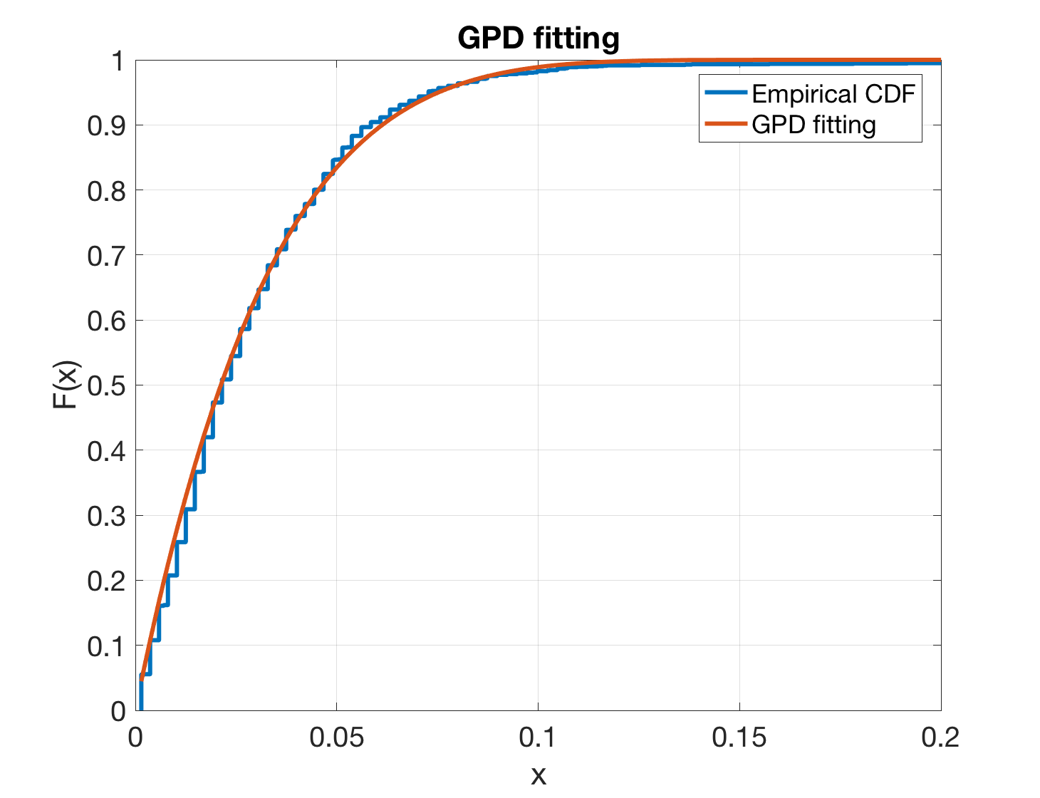
Figure 1. A comparison of cumulative distribution functions of empirical data $\{v_{i}\,|\,v_{i}>V\}$ and that of the generalized Pareto distribution.

Combining all estimates above, we obtain a bound

(4.2) $$\mathrm{d}_{w}(\pi,\hat{\pi})\leq 0.002350\,.$$

Since the invariant probability measure of equation 4.1 is known, we can check the sharpness of the bound given in equation (4.2). The approach we take is Monte Carlo simulation with extrapolation to infinite sample size. On a $256\times 256$ grid, we use $8$ long trajectories to estimate the invariant probability density function of 4.1. The sample sizes of these trajectories are $8\times 10^{8},1.6\times 10^{9},\cdots,6.4\times 10^{9}$. Then we compute the total variation distance between

$$u(x,y)=\frac{1}{K}e^{-2V(x,y)/\sigma^{2}}$$

and the empirical probability density function at those grid points. The error is linearly dependent on the $-1/2$ power of the sample size. Linear extrapolation shows that the total variation distance at the infinite sample limit is $\approx 0.001534$. The linear extrapolation is demonstrated in Figure 2. Since $\mathrm{d}_{w}$ is smaller than the total variation distance, the 1-Wasserstein distance $\mathrm{d}_{w}(\pi,\hat{\pi})$ should be no greater than $0.001534$. Therefore, our estimation given in equation (4.2) is larger than the true distance between $\pi$ and $\hat{\pi}$, but is reasonably sharp.

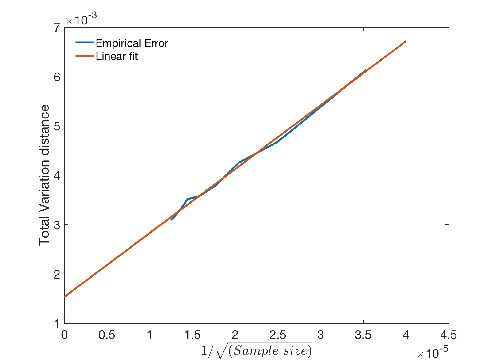
Figure 2. Linear extrapolation for the total variance distance $\|\pi-\hat{\pi}\|_{TV}$ at the infinite sample limit.

It remains to comment on the fast estimator mentioned in Section 3.3. In Figure 3 we draw the exponential tail of $\mathbb{P}[\tau_{c}>t]$ and its linear fit. The slope of the exponential tail is $\gamma=-0.1378$. When $T=10$, we have $e^{-\gamma T}=0.2521$. Equation (3.6) then gives an estimate

$$\mathrm{d}_{w}(\pi,\hat{\pi})\approx 0.00189377\,,$$

which is actually closer to the total variation distance that we have measured numerically.

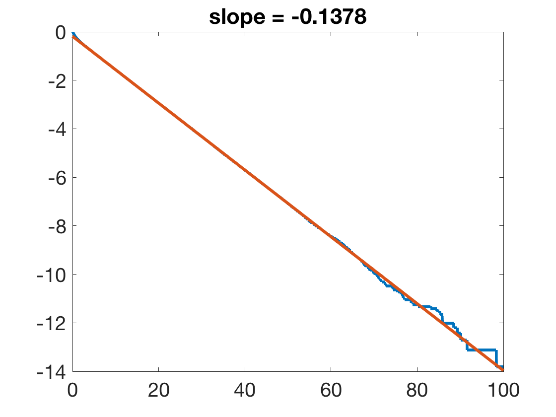
Figure 3. Exponential tail of $\mathbb{P}[\tau_{c}>t]$ versus $t$ when initial values are uniformly sampled in $\Omega\times\Omega$.

4.2. Double well potential

The second example we study is a gradient flow with respect to an asymmetric double well potential. Let

$$V(x)=\left\{\begin{array}[]{ll}6x^{2}-60&\mbox{ if }x\geq 4\\ \frac{1}{4}x^{4}-2x^{2}+4&\mbox{ if }0\leq x<4\\ \frac{1}{4}r^{4}x^{4}-2r^{2}x^{2}+4&\mbox{ if }-4/r\leq x<0\\ 6r^{2}x^{2}-60&\mbox{ if }x<-4/r\end{array}\right.$$

If $r\neq 1$, $V$ is an asymmetric double well potential function. Note that we make $V(x)$ a quadratic function when $x\geq 4$ or $x<-4/r$, because the original quartic function has very large derivatives when $|x|$ is large, which has some undesired numerical artifacts.

Now consider the gradient flow of $V(x)$ with additive random perturbation

$$X_{t}=-V^{\prime}(x)+\sigma\mathrm{d}W_{t}\,.$$

It is easy to see that $X_{t}$ admits an invariant probability measure $\pi$ with probability density function

$$u(x)=\frac{1}{K}e^{2V(x)/\sigma^{2}}\,,$$

where $K$ is a normalizer. In this example, we choose $\Omega=[-2,4]$, as $u(x)$ is extremely small when $x<-2$ or $x>4$.

Because of the double well potential, trajectories from two local minima need a long time to meet with one another. Hence the speed of convergence of the law of $X_{t}$ to $\pi$ is slow. Much longer times are needed so that trajectories can couple in Algorithm 2. In addition, we changed the underlying distance from $|x-y|$ to $|x-y|^{0.45}$, because if two initial values are very close to each other, with some small probability one trajectory can run into a different local minimum and takes a very long time to return. As a result, for reasonably large $T$, if the underlying distance $|x-y|$ is used, $\hat{P}^{T}$ does not contract in 1-Wasserstein metric space when two initial points are very close to each other.

Model parameters are chosen to be $r=5$, $\sigma=1.2$, and $T=50$. The numerical trajectory $\hat{X}_{t}$ is obtained by running Euler-Maruyama scheme with $h=0.0025$. We first run Algorithm 1 with $8$ independent long trajectories to compare the distance between $\hat{X}_{T}$ and $\hat{X}_{2h}$. The length of each trajectory is $5\times 10^{6}$. The constant $c$ is still equal to $1$ because the accuracy of Euler-Maruyama scheme is $O(h)$ when $\sigma$ is a constant. Algorithm 1 gives an upper bound

$$\mathrm{d}_{w}(\pi P^{T},\pi\hat{P}^{T})\leq 0.167345\,.$$

The upper bound is quite large due to large second order derivatives of $V(x)$ and large time span $T$.

Then we run Algorithm 2 to get the contraction rate of $\hat{P}^{T}$ for $T=50$. The number of initial values $(x_{i},y_{i})$ is $20000$. We run $1000$ pairs of trajectories from each initial points to get $\mathbb{P}[\tau_{c}>T]$. This gives $20000$ numbers

$$r_{i}=\frac{\mathbb{P}_{x_{i},y_{i}}[\tau_{c}>T]}{d(x_{i},y_{i})}\geq\frac{\mathrm{d}_{w}(\delta_{x_{i}}\hat{P}^{T},\delta_{y_{i}}\hat{P}^{T})}{d(x_{i},y_{i})}\,.$$

Then we use generalized Pareto distribution (GPD) to fit $\{1/(1-r_{i})\}_{i=1}^{20000}$. Similar to in the previous example, GPD parameter fitting gives $\alpha_{\Omega}=0.2019$. See Figure 4 Left for the fitting result. In addition, because this is an 1D problem, we can plot the contraction rate $r_{i}$ for each pair of $(x_{i},y_{i})$ on a grid that covers $\Omega\times\Omega$. See Figure 4 Right for a heat map of contraction rates from each pairs of initial points. From Figure 4 Right we can see that the high value of $\mathbb{P}_{x_{i},y_{i}}[\tau_{c}>T]$ is reached when one of the pairs $(x,y)$ falls into the left part of the domain, where $V(x)$ has large derivatives. In addition, when $(x,y)$ becomes even closer to line $\{x-y=0\}$, $\mathbb{P}_{x_{i},y_{i}}[\tau_{c}>T]$ drops dramatically to $0$. This further confirms that $\hat{P}^{T}$ is contracting in 1-Wasserstein metric space for $T=50$. Finally, we provide an exponential tail of $\mathbb{P}[\tau_{c}>t]$ for $\hat{X}_{t}$, demonstrated in Figure 5. The exponential tail is $\gamma=-0.09078$. Hence $e^{-\gamma T}$ gives $0.1068$, which is smaller than $\alpha_{\Omega}$ obtained above.

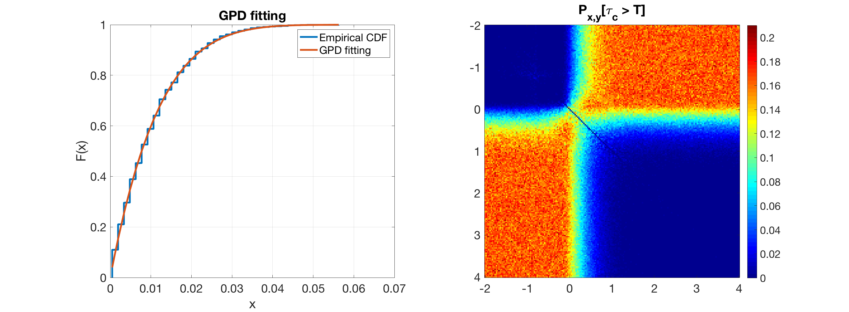
Figure 4. Left: Fitting generalized Paredo distribution with $v_{i}=1/(1-r_{i})$. The fitting result is compared with the empirical cumulative distribution function. Right: Heat map of contraction rate $r_{i}$ for initial pairs of points on a grid that covers $\Omega\times\Omega$.

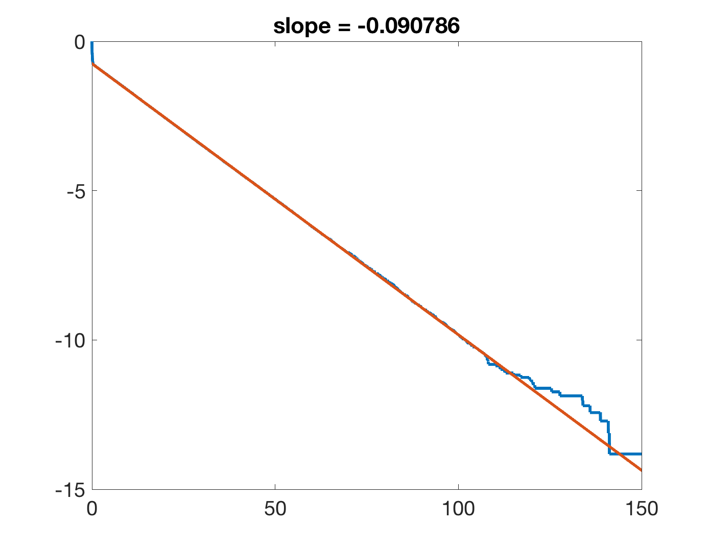
Figure 5. Exponential tail of $\mathbb{P}[\tau_{c}>t]$ versus $t$ when initial values are uniformly sampled in $\Omega\times\Omega$.

Combining all estimates above, we have an upper bound

(4.3) $$\mathrm{d}_{w}(\pi,\hat{\pi})\leq 0.2097\,.$$

If equation (3.6) is used instead, we have a rough estimate

$$\mathrm{d}_{w}(\pi,\hat{\pi})\approx 0.187354\,.$$

Both results imply that two invariant probability measures may be very different from each other. This can be confirmed by using Monte Carlo simulation to compute the invariant probability measure of $\hat{X}_{t}$. We run $8$ independent long trajectories of $\hat{X}_{t}$ up to $5\times 10^{6}$ to compute its invariant probability density function. The result is compared with $u(x)$, the invariant probability density function of $X_{t}$, in Figure 6. We can see visible difference between these two probability density functions. The total variation difference between them is $0.05906$. This is smaller than the bound predicted by equation (4.3), partially because we have to use the distance induced by $|x-y|^{0.45}$ to make $r_{i}$ uniformly bounded from above. But our calculation still predicts an unusually large difference between two invariant probability measures.

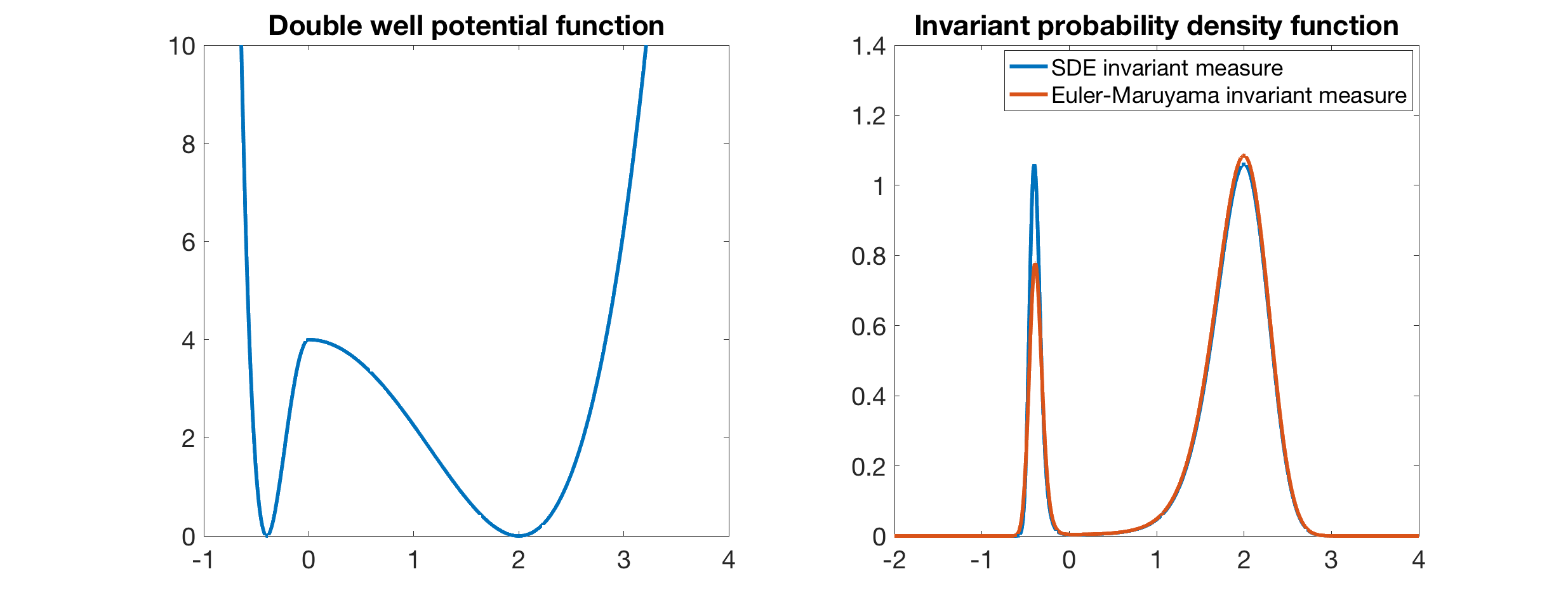
Figure 6. Left: potential function $V(x)$. Right: Comparison of invariant probability density functions of $X_{t}$ and $\hat{X}_{t}$.

We still owe readers a heuristic explanation of the phenomenon seen in Figure 6 Right. The probability density of the invariant probability measure of $\hat{X}_{t}$ is much lower than that of $X_{t}$ around the local minimum $x=-0.4$ because the potential function is asymmetric. As a result, when a trajectory of $\hat{X}_{t}$ moves from $x=-0.4$ to $x=0$, the Euler-Maruyama scheme tend to underestimate $-V^{\prime}(x)$, which increases dramatically near $x=-0.4$. The effect of such underestimation is much weaker near the other local minimum $x=2$, where the value of $|V^{\prime}(x)|$ is significantly smaller. As a result, it is easier for the trajectory of $\hat{X}_{t}$ to pass the separatrix $x=0$ from left to right than from right to left. This causes the unbalanced invariant probability density function as seen in Figure 6 Right.

4.3. Degenerate diffusion

Langevin dynamics have noise terms that only appear directly in the velocity equation and not on the position, leading to a Fokker-Planck equation with a degenerate, hypoelliptic diffusion. We consider a potential energy similar to the ring density equation, with SDE:

(4.4) $$\begin{split}dX&=V\,dt\\ dV&=-\nabla U(X)\,dt-\gamma V\,dt+\sigma\,dW\\ \end{split}$$

where

(4.5) $$U(X)=(X_{1}^{2}+X_{2}^{2}-1)^{2}.$$

One trajectory of equation (4.4) is demonstrated in Figure 7 Top Left. The invariant measure satisfies $\rho(X,V)\propto\exp(-\beta(V^{2}+U(X)))$ where $\beta=\frac{2\gamma}{\sigma^{2}}.$

Because of the degenerate noise term, we use a modified coupling algorithm involving three components which are based on the coupling in [14]. We consider two realizations $(X^{(1)},V^{(1)})$ and $(X^{(2)},V^{(2)})$ of the SDE and note that the difference process is contractive on the hyperplane $Q=X^{(1)}-X^{(2)}+\gamma^{-1}(V^{(1)}-V^{(2)})=0$ [14]. We employ reflection coupling when $\|Q\|>0.08,$ where the reflection tensor is given by $I-2*QQ^{T}/Q^{2}.$ When $\|Q\|<0.08,$ we use synchronized coupling, where both processes use the same realization of the Brownian noise. The threshold of switching coupling method (which is $0.08$ in our computation) should be $O(\sqrt{h})$, which is the distance that $(\hat{X}_{t},\hat{V}_{t})$ jumps after one step. When the processes are sufficiently close, we attempt to couple using maximal coupling using two steps of the numerical integrator. Two steps of the Euler-Maruyama integrator with stepsize $h$ gives

(4.6) $$\begin{split}X_{t+2h}&=X_{t}+2hV_{t}-h^{2}\nabla U(X_{t})-\gamma hV_{t}+\sigma h^{3/2}N_{0},\\ V_{t+2h}&=(1-\gamma h)^{2}V_{t}-(1-\gamma h)h\nabla U(X_{t})-h\nabla U(X_{t}+hV_{t})\\ &\qquad+\sigma(1-\gamma h)h^{1/2}N_{0}+\sigma h^{1/2}N_{1},\end{split}$$

where $N_{0}$ and $N_{1}$ represent two i.i.d. normal variables. We sample from the above to compute the probability of the processes to couple after two steps. To improve the computational efficiency of the scheme we only test for coupling when the processes are close, specifically, when $|X^{(1)}-X^{(2)}|<2.5\sigma h^{3/2}$ and $|V^{(1)}-V^{(2)}|<2.5\sigma h^{1/2}.$

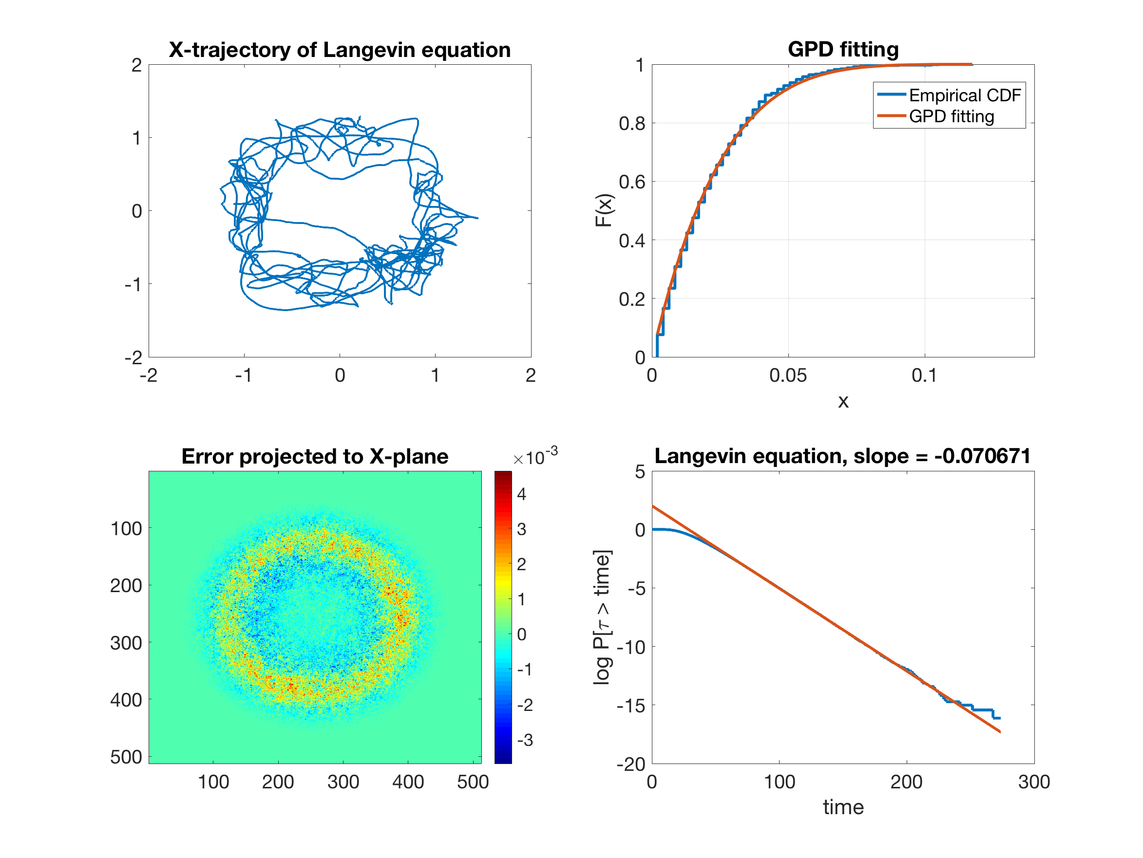
Figure 7. Top left: A sample path of Langevin equation with length $100$ (projected to X-plane). Top right: Fitting generalized Paredo distribution with $v_{i}=1/(1-r_{i})$. The fitting result is compared with the empirical cumulative distribution function. Bottom left: Difference between $\hat{\pi}$ and $\pi$ projected to X-plane. Bottom Right: Exponential tail of $\mathbb{P}[\tau_{c}>t]$ versus $t$ when initial values are uniformly sampled in $\Omega\times\Omega$.

In this simulation, we choose $\sigma=0.5$ and truncation time $T=40.$ The time step size is $h=0.001$. Averaged from $8$ long trajectories with length $4\times 10^{6},$ we find the error $d_{w}(\pi P^{T},\pi\hat{P}^{T})\leq 0.0111313.$ We choose the domain $\Omega=[-3\,,\,3]^{2}\times[-6\,,6]^{2}$ for the coordinates $(x_{1},x_{2},v_{1},v_{2})$. GPD fitting used $20,000$ pairs of initial values and $1,000$ trajectories for each pair of initial value giving $\alpha_{\Omega}=0.3727.$ See Figure 7 Top Right for a comparison of cumulative distribution function of the GPD fitting. This gives an upper bound

$$\mathrm{d}_{w}(\pi,\hat{\pi})\leq 0.017745\,.$$

It is not easy to numerically estimate the distance between $\pi$ and $\hat{\pi}$ as they are probability measures in $\mathbb{R}^{4}$. Instead, we project them to the $X$-plane and compare the projected probability density functions. Note that the difference between two projected probability density functions is smaller than that of $\pi$ and $\hat{\pi}$. In Figure 7 Bottom Left, we can see the difference between $P_{x}\hat{\pi}$ and $P_{x}\pi$, where $P_{x}$ is the projection operator to the $X$-plane. The approximate numerical invariant measure $\hat{\pi}$ in Figure 7 is obtained from $80$ long trajectories, each of which is integrated up to $T=10^{7}$. The probability density function of $\hat{\pi}$ is computed on a $512\times 512$ grid.

Finally, we compute the exponential tail of the coupling time to obtain the slope $\gamma=-0.07067$. Therefore, when $T=40$, equation (3.6) gives a rougher estimate

$$\mathrm{d}_{w}(\pi,\hat{\pi})\approx 0.011832\,.$$

4.4. Lorenz 96 model

In this subsection we study a highly chaotic example. Consider equation

(4.7) $$\mathrm{d}X^{1}_{t} =(X^{2}_{t}-X^{D-1}_{t})X^{D}_{t}-X^{1}_{t}+F+\sigma\mathrm{d}W^{1}_{t}$$

$$\mathrm{d}X^{2}_{t} =(X^{3}_{t}-X^{D}_{t})X^{1}_{t}-X^{2}_{t}+F+\sigma\mathrm{d}W^{2}_{t}$$

$$\vdots$$

$$\mathrm{d}X^{i}_{t} =(X^{i+1}_{t}-X^{i-2}_{t})X^{i-1}_{t}-X^{i}_{t}+F+\sigma\mathrm{d}W^{i}_{t},\quad i=3,\cdots,N-1$$

$$\vdots$$

$$\mathrm{d}X^{D}_{t} =(X^{1}_{t}-X^{D-2}_{t})X^{D-1}_{t}-X^{D}_{t}+F+\sigma\mathrm{d}W^{D}_{t}\,,$$

where the forcing term $F$ is usually chosen to be $8$. When $D=4$, the system has a large periodic orbits. It demonstrates chaotic dynamics when $D\geq 5$ [24]. See Figure 8 Left for the trajectory of the first three variables as an example.

In our simulations, we use Euler-Mayurama scheme with step size $h=0.0001$ to simulate numerical trajectories $\hat{X}_{t}$. Model parameters are $\sigma=3$ and $F=8$. The time span is chosen to be $T=3$. When $D=4$, in Algorithm 1, we run $8$ long trajectories with length $3\times 10^{5}$ each to compare the difference between $\hat{X}_{T}$ and $\hat{X}^{2h}_{T}$. The simulation gives an upper bound

$$\mathrm{d}_{w}(\pi P^{T},\pi\hat{P}^{T})\leq 0.144864\,.$$

Although we have chosen a small time step size $h$, this upper bound is still relatively large. The error gets even larger when $D=5$ is used, because the deterministic dynamics is intensively chaotic. The output of Algorithm 1 is $0.11946$ for $h=0.00001$ and $0.431059$ for $h=0.0001$.

Then we run Algorithm 2 for $D=4$ to get the contraction rate of $\hat{P}^{T}$ for $T=3$. $\Omega$ is chosen to be the 4D-box $[-16,\,19]^{4}$ because when running Algorithm 1, no trajectory has ever been outside of this box. The number of initial values $(x_{i},y_{i})$ is $20000$. We run $1000$ pairs of trajectories from each initial points to get $\mathbb{P}[\tau_{c}>T]$. This gives

$$r_{i}=\frac{\mathbb{P}_{x_{i},y_{i}}[\tau_{c}>T]}{d(x_{i},y_{i})}\geq\frac{\mathrm{d}_{w}(\delta_{x_{i}}\hat{P}^{T},\delta_{y_{i}}\hat{P}^{T})}{d(x_{i},y_{i})}$$

for $i=1,\cdots,20000$. The GPD fitting gives $\alpha_{\Omega}=0.7081$. See Figure 8 Right for the fitting result. Combine the output of two algorithms, we have the bound

$$\mathrm{d}_{w}(\pi,\hat{\pi})\leq 0.4963\,.$$

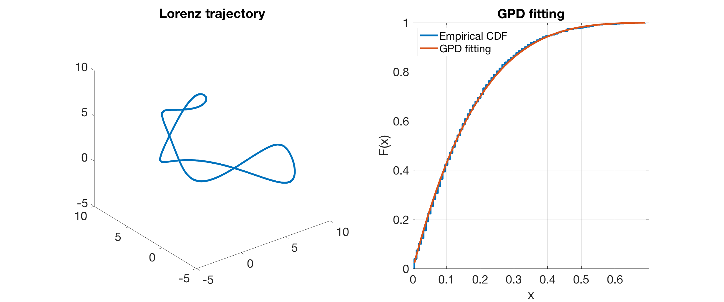
Figure 8. Left: A plot of the first 3 variables of the limit cycle. Right: GPD fitting of $\{1/(1-r_{i})\}_{i=1}^{20000}$ and a comparison with the empirical cumulative distribution function.

When $D=5$ and $h=1\times 10^{-5}$, the computational cost of Algorithm 2 becomes very high due to extremely small time step size. Instead, we compute exponential tails of the coupling time for $D=4$ and $D=5$ with $h=0.0001$. The result is demonstrated in Figure 9. We can see that when $D=5$, we have an exponential tail $\gamma=0.12541$. Therefore, if $T=3$ is unchanged, we have $(1-e^{-\gamma T})^{-1}=3.1892$. We conclude that when $D=5$, the 1-Wasserstein distance between $\pi$ and $\hat{\pi}$ is unacceptably large even if $h=1\times 10^{-5}$. This is mainly caused by very large finite time error. In order to approximate $\pi$ effectively, high order approximation of equation (4.7) is necessary.

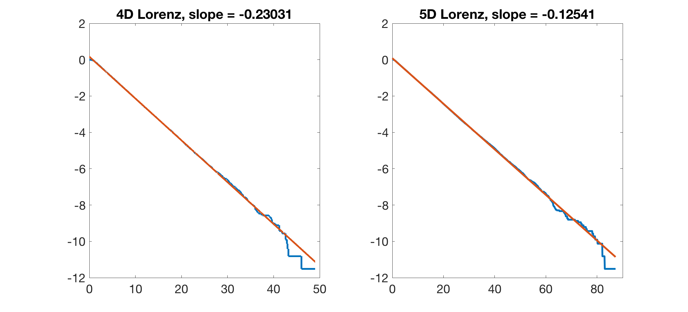
Figure 9. Exponential tail of $\mathbb{P}[\tau_{c}>t]$ versus $t$ when initial values are uniformly sampled in $\Omega\times\Omega$. Left: 4D Lorenz 96 system. Right: 5D Lorenz 96 system.

4.5. Stochastically coupled FitzHugh-Nagumo oscillator with mean-field interaction

We consider here a high dimensional example, a stochastically coupled FitzHugh-Nagumo(FHN) oscillator. FitzHugh-Nagumo model is a nonlinear model that models the periodic change of membrane potential of a spiking neuron under external stimulation. The model is a 2D system

(4.8) $$\mu\mathrm{d}u = (u-\frac{1}{3}u^{3}-v)\mathrm{d}t+\sqrt{\mu}\sigma\mathrm{d}W_{t}$$

$$\mathrm{d}v = (u+a)\mathrm{d}t+\sigma\mathrm{d}W_{t}\,,$$

where $u$ is the membrane potential, and $v$ is a recovery variable.

When $a=1.05$, the deterministic system admits a stable fixed point with a small basin of attraction [11]. A suitable random perturbation can drive this system away from the basin of attraction and trigger limit cycles intermittently.

In this section we consider $N$ coupled equations (4.8) with both nearest-neighbor interaction and mean-field interaction. Let $v=\sqrt{\mu}v$ be the new recovery variable. We have

(4.9) $$\mathrm{d}u_{i} =\left(\frac{1}{\mu}u-\frac{1}{3\mu}u^{3}-\frac{1}{\sqrt{\mu}}v+\frac{d_{u}}{\mu}(u_{i+1}+u_{i-1}-2u_{i})+\frac{w}{\mu}(\bar{u}-u_{i})\right)\mathrm{d}t+\frac{\sigma}{\sqrt{\mu}}\mathrm{d}W_{t}$$

$$\mathrm{d}v_{i} =(\frac{1}{\sqrt{\mu}}u+\frac{a}{\sqrt{\mu}})\mathrm{d}t+\frac{\sigma}{\sqrt{\mu}}\mathrm{d}W_{t}\,,$$

for $i=1,\cdots,N$, where $d_{u}$ is the neareast-neighbor coupling strength, $w$ is the mean field coupling strength, and

$$\bar{u}=\frac{1}{N}\sum_{i=1}^{N}u_{i}$$

is the mean membrane potential. In our simulations, we let $u_{-1}=u_{N}$ and $u_{N+1}=u_{1}$. In other words, $N$ neurons are connected as a ring.

The parameters we choose are $d_{u}=0.03$ and $w=0.3$. In addition we have $\sigma=0.6$. Activities of neurons are weakly coupled under this parameter set. See Figure 10 for the dynamics of this system. In particular, from Figure 10 Right, we can see that nearest neighbor neurons tend to spike together. However, the global dynamics is only weakly synchronized. The dimensions of system in our study are chosen to be $N=2$ and $N=40$, corresponding to stochastic differential equations in $\mathbb{R}^{4}$ and $\mathbb{R}^{80}$. The numerical scheme in our simulation is Euler-Maruyama scheme with $h=0.0005$. The finite time span is $T=3$ for both cases.

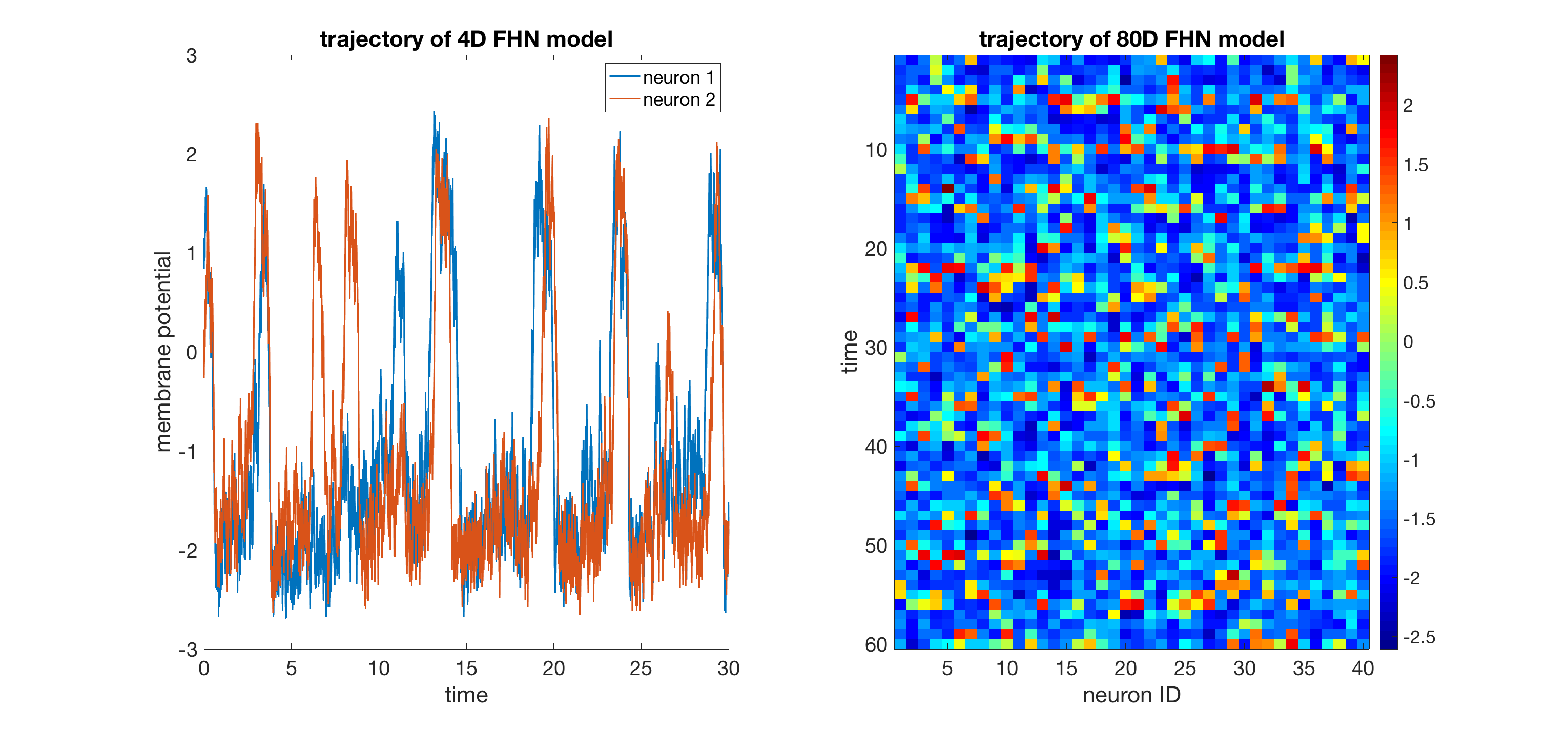
Figure 10. Dynamics of the FitzHugh-Nagumo model. Left: Trajectory of membrane potential of two neurons evolving along equation (4.9) with $N=2$ and other parameters specified in this paper. Right: Snapshots of membrane potential of $40$ neurons evolving along equation (4.9) with $N=40$ and other parameters specified in this paper.

We first run Algorithm 1 and Algorithm 2 for equation (4.9) with $N=2$. In Algorithm 1, we run $8$ long trajectories up to $3\times 10^{5}$. The simulation gives an upper bound

$$\mathrm{d}_{w}(\pi P^{T},\pi\hat{P}^{T})\leq 0.0105652$$

for $T=3$. Then we run Algorithm 2 for $\Omega=[-6,\,6]^{2N}$ to get the contraction rate of $\hat{P}^{T}$. The number of initial values is $40000$. This gives $40000$ coupling probabilities $r_{1},\cdots,r_{40000}$. Fitting these numbers with generalized Pareto distribution gives $\alpha_{\Omega}=0.5197$. See the result in Figure Figure 11 Left. Combine the output of two algorithms, we have

$$\mathrm{d}_{w}(\pi,\hat{\pi})\leq 0.0220\,.$$

Hence the invariant probability measure simulated by running the Euler-Maruyama scheme is trustworthy in spite of the presence of slow-fast dynamics. In addition, we compute the tail of coupling time for $N=2$, which is demonstrated in Figure 11 middle. The exponential tail has a slope $\gamma=0.50741$. Therefore, equation (3.6) gives an estimate

$$\mathrm{d}_{w}(\pi,\hat{\pi})\approx 0.01351\,.$$

When $N=40$, we still run Algorithm 1 with $8$ long trajectories up to time $3\times 10^{5}$. This gives us an estimate

$$\mathrm{d}_{w}(\pi P^{T},\pi\hat{P}^{T})\leq 0.0443737$$

for $T=3$. However, Algorithm 2 becomes expensive for $N=40$. Instead we compute the exponential of coupling time to get a rough estimate. The exponential tail of coupling time is demonstrated in Figure 11 Right. We have an exponential tail with slope $\gamma=0.31612$. Therefore, equation (3.6) gives a rough estimate

$$\mathrm{d}_{w}(\pi,\hat{\pi})\approx 0.07243\,.$$

Therefore, we conclude that $\hat{\pi}$ is an acceptable approximation of $\pi$ when $N=40$.

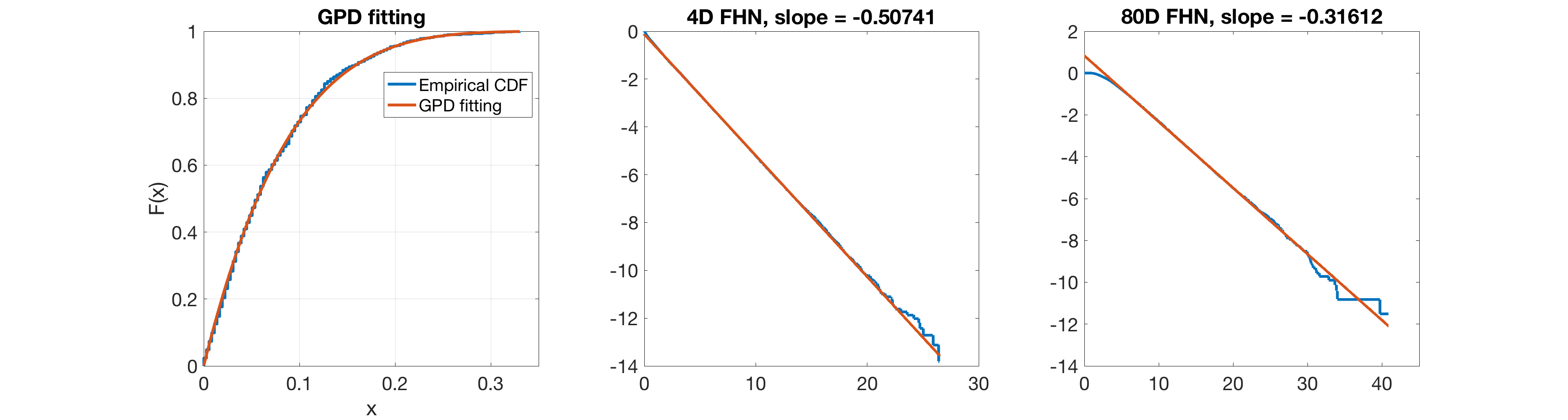
Figure 11. Left: GPD fitting of $\{1/(1-r_{i})\}_{i=1}^{40000}$ and a comparison with the empirical cumulative distribution function. Middle: Exponential tail of $\mathbb{P}[\tau_{c}>t]$ versus $t$ for equation (4.9) with $N=2$. Right: Exponential tail of $\mathbb{P}[\tau_{c}>t]$ versus $t$ for equation (4.9) with $N=40$.

5. Conclusion

In this paper we provide a coupling-based approach to quantitatively estimate the distance between the invariant probability measure $\pi$ of a stochastic differential equation (SDE) and that of its numerical scheme, denoted by $\hat{\pi}$. The key idea is that the distance $d(\pi,\hat{\pi})$ can be bounded by $\epsilon(1-\alpha)^{2}$, where $\epsilon$ is the finite time truncation error over the time interval $[0,T]$, and $\alpha$ is the rate of contraction of $\hat{P}^{T}$, the time-$T$ transition kernel of the numerical scheme for the SDE. The finite time truncation error comes from extrapolation analysis, and we use coupling method to estimate $\alpha$. Neither of these two estimates relies on spatial discretization. Hence our approach is relatively dimension free. Depending on the practical requirement, we provide one algorithm for computing a quantitative upper bound of $d(\pi,\hat{\pi})$, and an efficient algorithm for a “rough estimate” of $d(\pi,\hat{\pi})$. The performance of these two algorithms are tested with several numerical examples. Our approach can be extended to other stochastic processes, such as stochastic differential equations with random switching and applications related to Hamiltonian Monte Carlo [7, 33]. Also, our method is not limited to numerical analysis. In fact, $\hat{\pi}$ can be the invariant probability measure of any small perturbations of the original SDE. In this case, our method gives the sensitivity of $\pi$ against small perturbations.

This paper mainly estimates 1-Wasserstein distance between $\pi$ and $\hat{\pi}$. However, the coupling method can also be used to estimate the other type of distances, such as the total variation distance. In addition, in many cases, we are actually more interested in the error of the expectation of a certain observable when integrating with respect to $\hat{\pi}$ versus $\pi$. We choose 1-Wasserstein distance mainly because it is more convenient to estimate the finite time truncation error in 1-Wasserstein distance. In fact, there is only a small literature about estimating finite time truncation error in the total variation norm.

The difficulty of estimating finite time truncation error in total variation distance is partially solved if the grid-based SDE solver introduced in [8] is used. It is much easier to count samples on grids than in continuous state space. In fact, we find that this grid-based SDE solver is more compatible with both Fokker-Planck solver in [29, 12] and the sample quality checking algorithm studied in this paper. In the future, we will write a separate paper to discuss the application this sample quality checking algorithm to this grid-based SDE solver.

References

- [1] Christophe Andrieu, Nando De Freitas, Arnaud Doucet, and Michael I Jordan, An introduction to mcmc for machine learning, Machine learning 50 (2003), no. 1-2, 5–43.
- [2] Dominique Bakry and Michel Émery, Diffusions hypercontractives, Séminaire de Probabilités XIX 1983/84, Springer, 1985, pp. 177–206.
- [3] Turan G Bali, The generalized extreme value distribution, Economics letters 79 (2003), no. 3, 423–427.
- [4] A. Balkema and L. de Haan, Residual life time at great age, Annals of Probability 2 (1974), no. 5, 792–804.
- [5] Vlad Bally and Denis Talay, The law of the euler scheme for stochastic differential equations, Probability theory and related fields 104 (1996), no. 1, 43–60.
- [6] by same author, The law of the euler scheme for stochastic differential equations: Ii. convergence rate of the density, Monte Carlo Methods and Applications 2 (1996), no. 2, 93–128.
- [7] Nawaf Bou-Rabee, Andreas Eberle, and Raphael Zimmer, Coupling and convergence for hamiltonian monte carlo, arXiv preprint arXiv:1805.00452 (2018).
- [8] Nawaf Bou-Rabee and Eric Vanden-Eijnden, Continuous-time random walks for the numerical solution of stochastic differential equations, vol. 256, American Mathematical Society, 2018.
- [9] Enrique Castillo and Ali S Hadi, Fitting the generalized pareto distribution to data, Journal of the American Statistical Association 92 (1997), no. 440, 1609–1620.
- [10] Chuchu Chen, Jialin Hong, and Xu Wang, Approximation of invariant measure for damped stochastic nonlinear schrödinger equation via an ergodic numerical scheme, Potential Analysis 46 (2017), no. 2, 323–367.
- [11] Nan Chen, Andrew J Majda, and Xin T Tong, Spatial localization for nonlinear dynamical stochastic models for excitable media, arXiv preprint arXiv:1901.07318 (2019).
- [12] Matthew Dobson, Yao Li, and Jiayu Zhai, An efficient data-driven solver for fokker-planck equations: algorithm and analysis, submitted. arXiv:1906.02600, 2019.
- [13] Andreas Eberle, Reflection coupling and wasserstein contractivity without convexity, Comptes Rendus Mathematique 349 (2011), no. 19-20, 1101–1104.
- [14] Andreas Eberle, Arnaud Guillin, Raphael Zimmer, et al., Couplings and quantitative contraction rates for langevin dynamics, The Annals of Probability 47 (2019), no. 4, 1982–2010.
- [15] Mark Iosifovich Freidlin and Alexander D Wentzell, Random perturbations, Random Perturbations of Dynamical Systems, Springer, 1998, pp. 15–43.
- [16] Martin Hairer, Convergence of markov processes, Lecture notes (2010).
- [17] Martin Hairer and Jonathan C Mattingly, Yet another look at harris’ ergodic theorem for markov chains, Seminar on Stochastic Analysis, Random Fields and Applications VI, Springer, 2011, pp. 109–117.
- [18] Elton P Hsu and Karl-Theodor Sturm, Maximal coupling of euclidean brownian motions, Communications in Mathematics and Statistics 1 (2013), no. 1, 93–104.
- [19] Wen Huang, Min Ji, Zhenxin Liu, and Yingfei Yi, Steady states of Fokker-Planck equations: I. existence, Journal of Dynamics and Differential Equations 27 (2015), no. 3-4, 721–742.
- [20] by same author, Concentration and limit behaviors of stationary measures, Physica D: Nonlinear Phenomena 369 (2018), 1–17.
- [21] Pierre E Jacob, John O’Leary, and Yves F Atchadé, Unbiased markov chain monte carlo with couplings, arXiv preprint arXiv:1708.03625 (2017).
- [22] James E Johndrow and Jonathan C Mattingly, Error bounds for approximations of markov chains used in bayesian sampling, arXiv preprint arXiv:1711.05382 (2017).
- [23] Valen E Johnson, A coupling-regeneration scheme for diagnosing convergence in markov chain monte carlo algorithms, Journal of the American Statistical Association 93 (1998), no. 441, 238–248.
- [24] Alireza Karimi and Mark R Paul, Extensive chaos in the lorenz-96 model, Chaos: An interdisciplinary journal of nonlinear science 20 (2010), no. 4, 043105.
- [25] Rafail Khasminskii, Stochastic stability of differential equations, vol. 66, Springer Science & Business Media, 2011.
- [26] Peter E Kloeden and Eckhard Platen, Numerical solution of stochastic differential equations, vol. 23, Springer Science & Business Media, 2013.
- [27] Benedict Leimkuhler and Charles Matthews, Rational Construction of Stochastic Numerical Methods for Molecular Sampling, Applied Mathematics Research eXpress 2013 (2012), no. 1, 34–56.
- [28] Tony Lelievre and Gabriel Stoltz, Partial differential equations and stochastic methods in molecular dynamics, Acta Numerica 25 (2016), 681–880.
- [29] Yao Li, A data-driven method for the steady state of randomly perturbed dynamics, Communications in Mathematical Sciences, accepted (2019).
- [30] Yao Li and Yingfei Yi, Systematic measures of biological networks I: Invariant measures and entropy, Communications on Pure and Applied Mathematics 69 (2016), no. 9, 1777–1811.
- [31] Torgny Lindvall, Lectures on the coupling method, Courier Corporation, 2002.
- [32] Torgny Lindvall, L Cris G Rogers, et al., Coupling of multidimensional diffusions by reflection, The Annals of Probability 14 (1986), no. 3, 860–872.
- [33] Xuerong Mao and Chenggui Yuan, Stochastic differential equations with markovian switching, Imperial college press, 2006.
- [34] Jonathan C Mattingly, Andrew M Stuart, and Desmond J Higham, Ergodicity for sdes and approximations: locally lipschitz vector fields and degenerate noise, Stochastic processes and their applications 101 (2002), no. 2, 185–232.
- [35] Jonathan C Mattingly, Andrew M Stuart, and Michael V Tretyakov, Convergence of numerical time-averaging and stationary measures via Poisson equations, SIAM Journal on Numerical Analysis 48 (2010), no. 2, 552–577.
- [36] Sean P Meyn and Richard L Tweedie, Markov chains and stochastic stability, Springer Science & Business Media, 2012.
- [37] GN Milstein and MV Tretyakov, Computing ergodic limits for langevin equations, Physica D: Nonlinear Phenomena 229 (2007), no. 1, 81–95.
- [38] A Yu Mitrophanov, Sensitivity and convergence of uniformly ergodic markov chains, Journal of Applied Probability 42 (2005), no. 4, 1003–1014.
- [39] Chen Mufa, Estimation of spectral gap for markov chains, Acta Mathematica Sinica 12 (1996), no. 4, 337–360.
- [40] James III Pickands, Statistical inference using extreme order statistics, Annals of Statistics 3 (1975), no. 1, 119–131.
- [41] Gareth O Roberts, Richard L Tweedie, et al., Exponential convergence of langevin distributions and their discrete approximations, Bernoulli 2 (1996), no. 4, 341–363.
- [42] Daniel Rudolf, Nikolaus Schweizer, et al., Perturbation theory for markov chains via wasserstein distance, Bernoulli 24 (2018), no. 4A, 2610–2639.
- [43] Denis Talay, Second-order discretization schemes of stochastic differential systems for the computation of the invariant law, Stochastics: An International Journal of Probability and Stochastic Processes 29 (1990), no. 1, 13–36.
- [44] Denis Talay and Luciano Tubaro, Expansion of the global error for numerical schemes solving stochastic differential equations, Stochastic analysis and applications 8 (1990), no. 4, 483–509.