A structure-preserving approximation of the discrete split rotating shallow water equations

Abstract

We introduce an efficient split finite element (FE) discretization of a y-independent (slice) model of the rotating shallow water equations. The study of this slice model provides insight towards developing schemes for the full 2D case. Using the split Hamiltonian FE framework BaBeCo2019 (Bauer, Behrens and Cotter, 2019), we result in structure-preserving discretizations that are split into topological prognostic and metric-dependent closure equations. This splitting also accounts for the schemes’ properties: the Poisson bracket is responsible for conserving energy (Hamiltonian) as well as mass, potential vorticity and enstrophy (Casimirs), independently from the realizations of the metric closure equations. The latter, in turn, determine accuracy, stability, convergence and discrete dispersion properties. We exploit this splitting to introduce structure-preserving approximations of the mass matrices in the metric equations avoiding to solve linear systems. We obtain a fully structure-preserving scheme with increased efficiency by a factor of two.

1 Introduction

The notion of structure-preserving schemes describes discretizations that preserve important structures of the corresponding continuous equations: e.g. (i) the conservation of invariants such as energy, mass, vorticity and enstrophy in the case of the rotating shallow water (RSW) equations, (ii) the preservation of geometric structures such as div curl = curl grad = 0 or the Helmholtz decomposition of vector fields, and (iii) the conservation of large scale structures such as geostrophic or hydrostatic balances Staniforth2012 . Their conservation is important to avoid, for instance, biases in the statistical behavior of numerical solutions Franck2007 or to get models that correctly transfer energy and enstrophy between scales NataleCotter2017b .

The construction of such schemes is an active area of research and various approaches to develop structure-preserving discretizations exist: e.g. variational discretizations BaGB2018RSW ; BaGB2017AnPI ; PaMuToKaMaDe2010 or compatible FE methods CotterThuburn2012 ; McRaeCotter2014 . In particular FE methods are a very general, widely applicable approach allowing for flexible use of meshes and higher order approximations. When combined with Hamiltonian formulations, they allow for stable discretizations of the RSW equations that conserve energy and enstrophy BauerCotter2018 ; McRaeCotter2014 . However, they usually apply integration by parts to address the regularity properties of the FE spaces in use, which introduces additional errors and non-local differential operators. Moreover, FE discretizations usually involve mass matrices which are expensive to solve, while approximations of the mass matrices have to be designed carefully in order to preserve structure.

To address these disadvantages, we introduced in Bauer2017_1D ; BaBeCo2019 the split Hamiltonian FE method based on the split equations of GFD Bauer2016 , in which pairs of FE spaces are used such that integration by parts is avoided, and we derived structure-preserving discretizations of a y-independent RSW slice-model. Our method shares some basic ideas with mimetic discretizations (e.g. Beirao2017 ; Bochev2006 ; CotterThuburn2012 ; PalhaGerritsma2014 ) in which PDEs are written in differential forms, but stresses a distinction between topological and metric parts and the use of a proper FE space for each variable.

Here, we address the disadvantage of FE methods arising from mass matrices. In the framework of split FEM Bauer2017_1D ; BaBeCo2019 , we introduce approximations of the mass matrices in the metric equations resulting in a structure-preserving discretization of the split RSW slice-model that is more efficient that the original schemes introduced in BaBeCo2019 . To this end, we recall in Sect. 2 the split Hamiltonian framework and the split RSW slice-model, and we introduce the approximation of the metric equations. In Sect. 3, we present numerical results and in Sect. 4 we draw conclusions.

2 Split Hamiltonian FE discretization of the RSW slice-model

On the example of a y-independent slice model of the RSW equations, we recall the split Hamiltonian FE method of BaBeCo2019 . For pairs of height fields (straight 0-form $h^{(0)}$ and twisted 1-form $\widetilde{h}^{(1)}$), of velocity fields in $x$-direction (twisted 0-form $\widetilde{u}^{(0)}$ and straight 1-form $u^{(1)}$), and of velocity fields in outer slice direction (straight 0-form $v^{(0)}$ and twisted 1-form $\widetilde{v}^{(1)}$), this RSW slice-model reads

$$\begin{split}\frac{\partial u^{(1)}}{\partial t}-\tilde{\star}\widetilde{q}^{(0)}F_{v}^{(0)}+\operatorname{d}B^{(0)}=0,&\quad\frac{\partial\widetilde{v}^{(1)}}{\partial t}+\tilde{\star}\widetilde{q}^{(0)}\widetilde{F}_{u}^{(0)}=0,\quad\frac{\partial\widetilde{h}^{(1)}}{\partial t}+{\operatorname{d}}\widetilde{F}_{u}^{(0)}=0,\\ \widetilde{u}^{(0)}=\widetilde{\star}u^{(1)},&\qquad v^{(0)}=\widetilde{\star}\widetilde{v}^{(1)},\qquad\widetilde{h}^{(1)}=\widetilde{\star}h^{(0)},\end{split}$$ (1)

in which $\widetilde{F}_{u}^{(0)}:=h^{(0)}\widetilde{u}^{(0)}$ and $F_{v}^{(0)}:=h^{(0)}v^{(0)}$ are mass fluxes, $B^{(0)}:=gh^{(0)}+\frac{1}{2}(\widetilde{u}^{(0)})^{2}+\frac{1}{2}(v^{(0)})^{2}$ is the Bernoulli function with gravitational constant $g$, and $\widetilde{q}^{(0)}\widetilde{h}^{(1)}={\operatorname{d}}v^{(0)}+fdx$ with Coriolis parameter $f$ defines implicitly the potential vorticity (PV) $\widetilde{q}^{(0)}$. All variables are functions of $x$ and $t$: for instance, $u(x,t)$ is the coefficient function of the 1-form $u^{(1)}=u(x,t)dx$.

$$\begin{CD}h^{(0)},v^{(0)}\ \in\ \Lambda^{0}@>{\operatorname{d}}>{}>\Lambda^{1}\ \ni\ u^{(1)}\\ \hskip 45.52458pt@V{\tilde{\star}\,}V{}V@V{}V{\,\tilde{\star}}V\\ \widetilde{h}^{(1)},\widetilde{v}^{(1)}\ \in\ \widetilde{\Lambda}^{1}@<{\operatorname{d}}<{}<\widetilde{\Lambda}^{0}\ \ni\ \widetilde{u}^{(0)}\\ \end{CD}$$

Figure 1: Relation between operators and spaces.

The pairs of variables are connected via the twisted Hodge-star operator $\widetilde{\star}:\Lambda^{k}\rightarrow\widetilde{\Lambda}^{(1-k)}$ that maps from straight $k$-forms to twisted $(1-k)$-forms (or vice versa) with $k=0,1$ in one dimension (1D). The index ^(k) denotes the degree, and $\Lambda^{k},\widetilde{\Lambda}^{k}$ the space of all $k$-forms. Note that straight forms do not change their signs when the orientation of the manifold changes in contrast to twisted forms. The exterior derivative $\operatorname{d}$ is a mapping $\operatorname{d}:\Lambda^{k}\rightarrow\Lambda^{k+1}$ (or $\operatorname{d}:\widetilde{\Lambda}^{k}\rightarrow\widetilde{\Lambda}^{k+1}$). Here in 1D, it is simply the total derivative of a smooth function $g^{(0)}\in\Lambda^{0},\operatorname{d}g^{(0)}=\partial_{x}g(x)dx\in\Lambda^{1}$ (see Bauer2016 for full details). Diagram (1) illustrates the relations between the operators and spaces.

Galerkin discretization. To substitute FE for continuous spaces, we consider $\Lambda^{0}_{h},\widetilde{\Lambda}^{0}_{h}=CG_{p}$ and $\Lambda^{1}_{h},\widetilde{\Lambda}^{1}_{h}=DG_{p-1}$ with polynomial order $p$. The discrete Hodge star operators $\tilde{\star}_{h}^{0},\tilde{\star}_{h}^{1}$ map between straight and twisted spaces and may be non-invertible. The split FE discretization of Eqns. (1) seeks solutions $u_{h}^{(1)},\widetilde{v}_{h}^{(1)},\widetilde{h}_{h}^{(1)}\in(\Lambda^{1}_{h}(L),\widetilde{\Lambda}^{1}_{h}(L),\widetilde{\Lambda}^{1}_{h}(L))$ of the topological equations (as trivial projections)

$$\langle\chi_{h}^{(1)},\frac{\partial}{\partial t}u_{h}^{(1)}\rangle-\langle\chi_{h}^{(1)},\tilde{\star}\widetilde{q}_{h}^{(0)}F_{v_{h}}^{(0)}\rangle+\langle\chi_{h}^{(1)},\operatorname{d}B_{h}^{(0)}\rangle=0, \qquad\forall\chi_{h}^{(1)}\in\Lambda^{1}_{h},$$ (2)

$$\langle\widetilde{\chi}_{h}^{(1)},\frac{\partial\widetilde{v}_{h}^{(1)}}{\partial t}\rangle+\langle\widetilde{\chi}_{h}^{(1)},\tilde{\star}\widetilde{q}_{h}^{(0)}\widetilde{F}_{u_{h}}^{(0)}\rangle=0, \qquad\forall\widetilde{\chi}_{h}^{(1)}\in\widetilde{\Lambda}^{1}_{h},$$ (3)

$$\langle\widetilde{\chi}_{h}^{(1)},\frac{\partial\widetilde{h}_{h}^{(1)}}{\partial t}\rangle+\langle\widetilde{\chi}_{h}^{(1)},\operatorname{d}\widetilde{F}_{u_{h}}^{(0)}\rangle=0, \qquad\forall\widetilde{\chi}_{h}^{(1)}\in\widetilde{\Lambda}^{1}_{h},$$ (4)

$$\langle\tilde{\star}\widetilde{\phi}_{h}^{(0)},\widetilde{q}_{h}^{(0)}\widetilde{h}_{h}^{(1)}\rangle-\langle\tilde{\star}\widetilde{\phi}_{h}^{(0)},\operatorname{d}v_{h}^{(0)}\rangle-\langle\tilde{\star}\widetilde{\phi}_{h}^{(0)},fdx\rangle=0, \qquad\forall\widetilde{\phi}_{h}^{(0)}\in\widetilde{\Lambda}^{0}_{h},$$ (5)

subject to the metric closure equations (as non-trivial Galerkin projections (GP))

$$\begin{split}\widetilde{u}^{(0)}=\widetilde{\star}u^{(1)}\approx{\rm GP}(1-i)_{u}:\langle\widetilde{u}_{h}^{(0)}(x),\hat{\tau}^{i}(x)\rangle&=\langle u_{h}^{(1)}(x),\hat{\tau}^{i}(x)\rangle\,,\ \forall\hat{\tau}^{i}\in\hat{\Lambda}_{h}^{i},\\ v^{(0)}=\widetilde{\star}\widetilde{v}^{(1)}\approx{\rm GP}(1-i)_{v}:\langle v_{h}^{(0)}(x),\hat{\tau}^{i}(x)\rangle&=\langle\widetilde{v}_{h}^{(1)}(x),\hat{\tau}^{i}(x)\rangle\,,\ \forall\hat{\tau}^{i}\in\hat{\Lambda}_{h}^{i},\\ \widetilde{h}^{(1)}=\widetilde{\star}h^{(0)}\approx{\rm GP}(1-i)_{h}:\langle h_{h}^{(0)}(x),\hat{\tau}^{j}(x)\rangle&=\langle\widetilde{h}_{h}^{(1)}(x),\hat{\tau}^{j}(x)\rangle\,,\ \forall\hat{\tau}^{j}\in\hat{\Lambda}_{h}^{j},\end{split}$$ (6)

for $i,j=0,1$. $\langle\cdot,\cdot\rangle:=\int_{L}\cdot\wedge\tilde{\star}\cdot$ is the $L_{2}$ inner product on the domain $L$. We distinguish between continuous and discrete Hodge star operators $\tilde{\star}$ and $\tilde{\star}_{h}$, respectively. $\tilde{\star}$ is used in $\langle,\rangle$ such that $k$-forms of the same degree are multiplied, which translates into a standard inner product for coefficient functions: e.g. $\langle\tilde{\star}u_{h}^{(1)},\widetilde{u}_{h}^{(0)}\rangle=\langle u_{h}^{(1)}(x),\widetilde{u}_{h}^{(0)}(x)\rangle$. $\tilde{\star}_{h}$ is realized as in Eqns. (6) via non-trivial GP between 0- and 1-forms, cf. Bauer2017_1D .

2.1 Continuous and discrete split Hamiltonian RSW slice-model

Both the continuous split RSW slice-model of Eqns. (1) and the corresponding weak (discrete) form of (2)–(6) can equivalently be written in Hamiltonian form, as shown in BaBeCo2019 . Considering the discrete version, the Hamiltonian with metric equations reads

$$\begin{split}\mathcal{H}[u_{h}^{(1)},\widetilde{v}_{h}^{(1)},\widetilde{h}_{h}^{(1)}]&=\frac{1}{2}\langle u_{h}^{(1)},{\tilde{\star}}h_{h}^{(0)}\widetilde{u}_{h}^{(0)}\rangle+\frac{1}{2}\langle\widetilde{v}_{h}^{(1)},{\tilde{\star}}h_{h}^{(0)}v_{h}^{(0)}\rangle+\langle\widetilde{h}_{h}^{(1)},{\tilde{\star}}gh_{h}^{(0)}\rangle\\ &\widetilde{u}_{h}^{(0)}=\tilde{\star}_{h}u_{h}^{(1)},\ v_{h}^{(0)}=\tilde{\star}_{h}\widetilde{v}_{h}^{(1)},\ h_{h}^{(0)}=\tilde{\star}_{h}\widetilde{h}_{h}^{(1)}\ \text{(metric eqns.)}\end{split}$$ (7)

while the almost Poisson bracket $\{,\}$ is defined as

$$\{\mathcal{F},\mathcal{G}\}:=-\langle\frac{\delta\mathcal{F}}{\delta\widetilde{h}_{h}^{(1)}},\operatorname{d}\tilde{\star}\frac{\delta\mathcal{G}}{\delta u_{h}^{(1)}}\rangle-\langle\frac{\delta\mathcal{F}}{\delta u_{h}^{(1)}},\operatorname{d}\tilde{\star}\frac{\delta\mathcal{G}}{\delta\widetilde{h}_{h}^{(1)}}\rangle+\langle\frac{\delta\mathcal{F}}{\delta u_{h}^{(1)}},\tilde{\star}{\widetilde{q}_{h}^{(0)}}\tilde{\star}\frac{\delta\mathcal{G}}{\delta\widetilde{v}_{h}^{(1)}}\rangle-\langle\frac{\delta\mathcal{F}}{\delta\widetilde{v}_{h}^{(1)}},\tilde{\star}{\widetilde{q}_{h}^{(0)}}\tilde{\star}\frac{\delta\mathcal{G}}{\delta u_{h}^{(1)}}\rangle$$ (8)

with PV defined by: $\langle\tilde{\star}\widetilde{\phi}_{h}^{(0)},\widetilde{q}_{h}^{(0)}\widetilde{h}_{h}^{(1)}\rangle+\langle\operatorname{d}\widetilde{\phi}_{h}^{(0)},\widetilde{v}_{h}^{(1)}\rangle-\langle\tilde{\star}\widetilde{\phi}_{h}^{(0)},fdx\rangle=0,\ \forall\widetilde{\phi}_{h}^{(0)}\in\widetilde{\Lambda}^{0}_{h}$. Then, the dynamics for any functional $\mathcal{F}[u_{h}^{(1)},\widetilde{v}_{h}^{(1)},\widetilde{h}_{h}^{(1)}]$ is given by $\frac{d}{dt}\mathcal{F}=\{\mathcal{F},\mathcal{H}\}$.

Splitting of schemes properties. The split Hamiltonian FE method results in a family of schemes in which the schemes’ properties split into topological and metric dependent ones, cf. BaBeCo2019 .

The topological properties hold for all double FE pairs that fulfill commuting diagram (1). In particular,

• the total energy is conserved, because $\frac{d}{dt}\mathcal{H}=\{\mathcal{H},\mathcal{H}\}=0$ which follows from the antisymmetry of (8);

• the Casimirs $\mathcal{C}=M,PV,PE$ are conserved as $\frac{d}{dt}\mathcal{C}=\{\mathcal{C},\mathcal{H}\}=0$ for $\{\mathcal{C},\mathcal{G}\}=0\forall\mathcal{G}$ with $\mathcal{C}=\langle\widetilde{h}_{h}^{(1)},{\tilde{\star}}F(\widetilde{q}_{h}^{(0)})\rangle$ for $F=1(M)$, $F=\widetilde{q}_{h}^{(0)}\tilde{1}(PV)$, $F=(\widetilde{q}_{h}^{(0)})^{2}(PE)$;

• {, } is independent of $\tilde{\star}_{h}$, hence $\mathcal{H},\mathcal{C}$ are conserved for any metric equation.

The metric properties are associated to a certain choice of FE spaces. In particular, this choice determines

• the dispersion relation which usually depends on $\Delta x$ between DoFs,

• the stability, because the inf-sub condition depends on the norm, and

• convergence and accuracy, which both are measured with respect to norms.

2.2 Family of structure-preserving split RSW schemes

Besides the splitting into topological and metric properties, another remarkable feature of the split FE framework is that one choice of compatible FE pairs leads to a family of split schemes, cf. Bauer2017_1D ; BaBeCo2019 . In the following, we consider for $p=1$ the piecewise linear space $\Lambda^{0}_{h},\widetilde{\Lambda}^{0}_{h}=CG_{p}={\rm P}1$ with basis $\{\phi_{l}(x)\}_{{{l}}=1}^{N}$ and the piecewise constant space $\Lambda^{1}_{h},\widetilde{\Lambda}^{1}_{h}=DG_{p-1}={\rm P}0$ with basis $\{\chi_{m}(x)\}_{{{m}}=1}^{N}$. Being in a 1D domain with periodic boundary, both have $N$ independent DoFs. We approximate 0-forms in P0 and 1-forms in P1, e.g. $u_{h}^{(1)}(x,t)=\sum_{{{m}}=1}^{N}u_{m}(t)\chi_{m}(x)$. The split framework BaBeCo2019 leads to one set of discrete topological equations for Eqn. (2)–(5), and four combinations of discrete metric equations for (6):

$$\text{{topol. momentum eqn.:}}\hskip 9.00002pt\frac{\partial}{\partial t}{\bf u}^{1}_{e}+{\bf D}^{en}{\bf B}^{0}_{n}-\widetilde{{\bf M}^{en}}({\bf\tilde{q}}^{0}_{n}\circ{\bf F}^{v}_{n})=0,\ \frac{\partial}{\partial t}{\bf\tilde{v}}^{1}_{e}+\widetilde{{\bf M}^{en}}({\bf\tilde{q}}^{0}_{n}\circ{\bf\tilde{F}}^{u}_{n})=0,$$

$$\text{{topol. continuity eqn.:}}\hskip 186.30028pt\frac{\partial}{\partial t}{\bf\tilde{h}}^{1}_{e}+{\bf D}^{en}{\bf\tilde{F}}^{u}_{n}=0,$$

$$\text{{metric closure eqn.:}}\hskip 13.50002pt\begin{CD}{\bf h}^{0}_{n}\quad\in\quad\Lambda^{0}_{h}{\subset P1}@>{{\bf D}^{en}}>{}>\Lambda^{1}_{h}{\subset P0}\quad\ni\quad{\bf u}^{1}_{e},({\bf\tilde{v}}^{1}_{e}\in\widetilde{\Lambda}^{1}_{h})\\ \hskip 34.14322pt@V{{{{\rm GP1}_{h}:}\ {\bf M}^{nn}{\bf h}^{0}_{n}={\bf P}^{ne}{\bf\tilde{h}}^{1}_{e}}}V{}V@V{}V{{{{\rm GP1}_{u}:}\ {\bf M}^{nn}{\bf\tilde{u}}^{0}_{n}={\bf P}^{ne}{\bf u}^{1}_{e}\ \&\ {\bf M}^{nn}{\bf v}^{0}_{n}={\bf P}^{ne}{\bf\tilde{v}}^{1}_{e}}}V\\ \hskip 34.14322pt@V{{{{\rm GP0}_{h}:}\ {\bf M}^{en}{\bf h}^{0}_{n}={\bf\tilde{h}}^{1}_{e}\,\quad}}V{}V@V{}V{{{{\rm GP0}_{u}:}\ {\bf M}^{en}{\bf\tilde{u}}^{0}_{n}={\bf u}^{1}_{e}\ \ \,\&\ \,{\bf M}^{en}{\bf v}^{0}_{n}={\bf\tilde{v}}^{1}_{e}}}V\\ {\bf\tilde{h}}^{1}_{e}\quad\in\quad\widetilde{\Lambda}^{1}_{h}{\subset P0}@<{{\bf D}^{en}}<{}<\widetilde{\Lambda}^{0}_{h}{\subset P1}\quad\ni\quad{\bf\tilde{u}}^{0}_{n},({\bf v}^{0}_{n}\in\Lambda^{0}_{h}).\\ \end{CD}$$ (9)

Here, we used the following $(N\times N)$ matrices with index $n$ for nodes and $e$ for elements: (i) mass matrices ${\bf M}^{nn}$, ${\bf M}^{ee}$, ${\bf M}^{en}$, with metric-dependent coefficients $({\bf M}^{nn})_{{{l}}{{l^{\prime}}}}=\int_{L}\phi_{l}(x)\phi_{l^{\prime}}(x)dx$, $({\bf M}^{ee})_{{{m}}{{m^{\prime}}}}=\int_{L}\chi_{m}(x)\chi_{m^{\prime}}(x)dx$, $({\bf M}^{en})_{{{l}}{{m^{\prime}}}}=\int_{L}\phi_{l}(x)\chi_{m^{\prime}}(x)dx$ (with $\widetilde{{\bf M}^{en}}=\{{\bf M}^{en}\text{in Or},-{\bf M}^{en}\text{in -Or}\}$ for orientation Or of $L$ and ${\bf M}^{en}=({\bf M}^{ne})^{T}$ with $T$ for the transposed matrix); and (ii) the stiffness matrix ${\bf D}^{en}$ with metric-independent coefficient $({\bf D}^{en})_{{{l}}{{m^{\prime}}}}=\int_{L}\frac{d\phi_{l}(x)}{dx}\chi_{m^{\prime}}(x)dx$ (with ${\bf D}^{en}=({\bf D}^{ne})^{T}$). We separate ${\bf M}^{ne}={\bf P}^{ne}\,({\bf\Delta x}_{e})^{T}$ into a metric-dependent ${\bf\Delta x}_{e}$ and a metric-free part ${\bf P}^{ne}$, the latter is an averaging operator from $e$ to $n$ values.

Considering the discrete variables, ${\bf u}^{1}_{e}={\bf M}^{ee}{\bf u}_{e}$ is a discrete 1-form associated to the vector array ${\bf u}_{e}=\{u_{m}(t)|m=1,...N\}$, analogously for ${\bf\tilde{v}}^{1}_{e}$. Similarly, ${\bf\tilde{h}}^{1}_{e}={\bf M}^{ee}{\bf\tilde{h}_{e}}$ is a discrete 1-from with ${\bf\tilde{h}}_{e}=\{\widetilde{h}_{m}(t)|m=1,...N\}$. Discrete 0-forms read, e.g. ${\bf h}^{0}_{n}=\{h_{l}(t)|l=1,...N\}$. The discrete mass fluxes are ${\bf\tilde{F}}^{u}_{n}={\bf h}^{0}_{n}\circ{\bf\tilde{u}}^{0}_{n}\quad\text{and}\quad{\bf F}^{v}_{n}={\bf h}^{0}_{n}\circ{\bf v}^{0}_{n}$ and the discrete Bernoulli function reads ${\bf B}^{0}_{n}=\frac{1}{2}{\bf\tilde{u}}^{0}_{n}\circ{\bf\tilde{u}}^{0}_{n}+\frac{1}{2}{\bf v}^{0}_{n}\circ{\bf v}^{0}_{n}+g{\bf h}^{0}_{n}$. Finally, ${\rm GP1}_{u},{\rm GP0}_{u},{\rm GP1}_{h},{\rm GP0}_{h}$ are the nonlinear GPs of (6) for P1 and P0 test functions.

2.3 A structure-preserving approximation of split RSW schemes

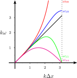
Figure 2: Dispersion relations: analytic (black) for $c=\sqrt{gH}=1$, $\omega_{00}$ (green) for ${\rm GP1}_{u}$-${\rm GP1}_{h}$, $\omega_{01}$ (blue) for ${\rm GP1}_{u}$-${\rm GP0}_{h}$ and ${\rm GP0}_{u}$-${\rm GP1}_{h}$, $\omega_{11}$ (red) for ${\rm GP0}_{u}$-${\rm GP0}_{h}$ (cf. BaBeCo2019 ), and $\omega_{aa}$ (magenta) for ${\rm AVG}_{u}$-${\rm AVG}_{h}$.

Here we introduce a new, computationally more efficient split RSW scheme compared to those of BaBeCo2019 . We exploit the splitting of the topological and metric properties within the split FE framework to introduce structure-preserving approximations of the mass matrices used in the metric equations. Instead of using the full nontrivial Galerkin projections ${\rm GP1}_{h},{\rm GP0}_{h}$ for height or ${\rm GP1}_{u},{\rm GP0}_{u}$ for velocity $u,v$, we use the averaged versions:

$${\rm AVG}_{h}:{\bf h}^{0}_{n}=\mathbf{A}^{en}{\bf\tilde{h}}^{1}_{e}\,,\quad{\rm AVG}_{u}:{\bf\tilde{u}}^{0}_{n}=\mathbf{A}^{en}{\bf u}^{1}_{e}\,,$$

with averaging operator $\mathbf{A}^{en}=({\bf P}^{ne})^{T}$ and denote the resulting scheme with ${\rm AVG}_{u}$-$\,{\rm AVG}_{h}$. Rather then solving linear systems in (9), we obtain values for ${\bf h}^{0}_{n},{\bf\tilde{u}}^{0}_{n},{\bf v}^{0}_{n}$ simply by averaging. This is computationally more efficient. In fact, already for this 1D problem we achieve a speedup by a factor of 2 (wall clock time) compared to the full GPs.

As stated in Sect. 2.1, such modification does not impact on the structure-preserving properties but will change the metric-dependent ones instead. Before we confirm this in Sect. 3 numerically, we first determine analytically the discrete dispersion relation related to this approximation. A similar calculation as done in Bauer2017_1D leads to the following discrete dispersion relation:

$$c_{d}=\frac{\omega_{aa}}{k}=\pm\sqrt{gH}\frac{1}{k\Delta x}\sin(k\Delta x)$$

with angular frequency $\omega_{aa}=\omega_{aa}(k)$ and discrete wave speed $c_{d}\rightarrow c=\sqrt{gH}$ (with mean height $H$) in case $k\rightarrow 0$ and with a spurious mode (second zero root) at shortest wave length $k=\frac{\pi}{\Delta x}$. As shown in Fig. 2 (with results relative to the nondimensional wave speed $c=\sqrt{gH}=1$), this is similar to the dispersion relation of the ${\rm GP1}_{u}$-${\rm GP1}_{h}$ scheme in the sense that both have a spurious mode at $k=\frac{\pi}{\Delta x}$, cf. Bauer2017_1D . For completeness, we added the dispersion relation for the other possible realizations of the metric equations (9) as introduced in Bauer2017_1D ; BaBeCo2019 .

3 Numerical results

We study the structure-preserving properties, as well as convergence, stability and dispersion relation for the averaged split scheme ${\rm AVG}_{u}$-$\,{\rm AVG}_{h}$ and compare it with the split schemes of BaBeCo2019 . We use test cases (TC) in the quasi-geostrophic regime such that effects of both gravity waves and compressibility are important.

The study of structure preservation (topological properties) will be performed with a flow in geostrophic balance in which the terms are linearly balanced while nonlinear effects are comparably small (Fig. 3). To illustrate the long term behaviour, we run the simulation in this TC 1 for about 10 cycles (meaning that the (analytical) wave solutions have traveled 10 times over the entire domain). To test convergence and stability (i.e. metric-dependent properties), we use in TC 2 a steady state solutions of Eqn. (1). To illustrate the metric dependency of the dispersion relations, we use in TC 3 an initial height distribution (as in Fig. 3, left) that is only partly in linear geostrophic balance such that shock waves with small scale oscillations develop that depend on the dispersion relation. More details on the TC can be found in BaBeCo2019 .

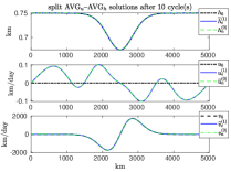
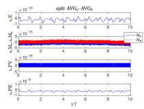
Figure 3: Solutions for the split ${\rm AVG}_{u}$-$\,{\rm AVG}_{h}$ scheme for a mesh with 512 elements. Initial fields are shown as dashed-dotted lines. Left: flow in geostrophic balance after 10 cycles. Right: time series of the quantities of interest for 10 cycles.

Topological properties. Figure 4 (left) shows for TC 1 the relative errors of the averaged split scheme for energy $E$, mass $M_{e}$ or $M_{n}$, potential vorticity $PV$ and enstrophy $PE$ (see definitions in BaBeCo2019 ). In all cases studied, $M_{e},M_{n}$ and $PV$ are preserved at machine precision. For $512$ elements, the error in $E$ is at the order of $10^{-10}$ while for $PE$ it is at $10^{-9}$. With higher mesh resolution, the errors decrease with third order rate (Fig. 4, left).

When compared to the split schemes of BaBeCo2019 , these error values are very close to the results presented therein, underpinning the fact that modifications in the metric equations do not affect the quality of structure preservation of the schemes.

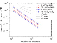
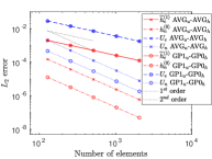
Figure 4: Relative error values in dependence of $N$ of ${\rm AVG}_{u}$-$\,{\rm AVG}_{h}$ compared to ${\rm GP1}_{u}$–$\,{\rm GP0}_{h}$. Left: errors for $E$ and $PE$ for TC 1. Right: errors for the steady state solution of TC 2 after 1 cycle.

Metric-dependent properties. Consider next the convergence behaviour of the averaged split scheme ${\rm AVG}_{u}$-$\,{\rm AVG}_{h}$ shown in Figure 4 (right) for TC 2. To ease comparison, we include $L_{2}$ error values of the split scheme ${\rm GP1}_{u}$–$\,{\rm GP0}_{h}$ of BaBeCo2019 noting that the other split schemes presented therein share more or less the same error values for the corresponding fields. In all cases, the error values decrease as expected: all P1 fields show second order, all P0 fields first order convergences rates.

While the errors of the P0 fields of ${\rm AVG}_{u}$–$\,{\rm AVG}_{h}$ is close to the corresponding values of the split schemes of BaBeCo2019 , the P1 fields of ${\rm AVG}_{u}$–$\,{\rm AVG}_{h}$ have error values that are about one order of magnitude large than the corresponding fields of e.g. ${\rm GP1}_{u}$–$\,{\rm GP0}_{h}$. This agrees well with the fact that we do not solve the full linear system in the metric equations to recover the P1 fields but use instead approximations, which slightly increases the P1 error values of ${\rm AVG}_{u}$–$\,{\rm AVG}_{h}$.

\begin{overpic}[scale={0.3},unit=1mm]{fig_avg_tc3zoom_fields_vAVG_hAVG_H075_N512_0d225_large.pdf} \put(45.0,40.0){\includegraphics[scale={.205}]{fig_tc3bzoom_fields_v1h1_H075_N512_0d225.pdf}} \put(80.0,20.0){\includegraphics[scale={.205}]{fig_tc3bzoom_fields_v0h1_H075_N512_0d225.pdf}} \put(115.0,0.0){\includegraphics[scale={.205}]{fig_tc3bzoom_fields_v0h0_H075_N512_0d225.pdf}} \put(15.0,50.0){${\color[rgb]{1,0,1}\omega_{aa}}$} \put(155.0,40.0){${\color[rgb]{1,0,0}\omega_{00}}$} \put(125.0,60.0){${\color[rgb]{0,0,1}\omega_{01}}$} \put(90.0,80.0){${\color[rgb]{0,1,0}\omega_{11}}$} \end{overpic}                          \begin{overpic}[scale={0.30},unit=1mm]{fig_avg_tc3zoom_Vfields_vAVG_hAVG_H075_N512_0d225_large.pdf} \end{overpic}

Figure 5: Fields with oscillations at the wave fronts in dependency of the wave dispersion relations of Fig. 2 on a mesh with $N_{e}=512$ elements and after a simulation time of $0.225$ cycles.

With TC 3 we illustrate numerically how the choice of metric equations determines the discrete dispersion relations. As derived in Sect. 3, the discrete dispersion relation of ${\rm AVG}_{u}$–$\,{\rm AVG}_{h}$ equals a sine wave, hence all waves of frequency $k$ have wave speeds equal or slower than $c$ (black curve in Fig. 2). In particular for wave numbers larger then $\frac{\pi}{2\Delta x}$, waves start to slow down until there is a standing wave at $k=\frac{\pi}{\Delta x}$. This is a similar behavior to the ${\rm GP1}_{u}$–$\,{\rm GP1}_{h}$ scheme of BaBeCo2019 , but for ${\rm AVG}_{u}$–$\,{\rm AVG}_{h}$ this effect is stronger given the generally slower wave propagation. This behaviour is clearly visible in Figure 5 where we observe in both fields lower frequency oscillation behind the front when compared to ${\rm GP1}_{u}$–$\,{\rm GP1}_{h}$ (see inlet). This result agrees well with the discrete dispersion relations shown in Fig. 2.

4 Conclusions

We introduced a y-independent RSW slice-model in split Hamiltonian form and derived a family of lowest-order (P0-P1) structure-preserving split schemes. The splitting of the equations into topological and metric parts transfers also to schemes’ properties. The framework allows for different realizations of metric equations which all preserve the Hamiltonian and the Casimirs of the Poisson bracket. This allowed us to introduce an approximation of the metric equations which is structure-preserving, achieving a speedup of a factor of 2 because no linear systems had to be solved.

References

• (1) Bauer, W. [2016], A new hierarchically-structured n-dimensional covariant form of rotating equations of geophysical fluid dynamics, GEM - Intern. J. Geomathematics, 7(1), 31–101.
• (2) Bauer, W., Cotter, C. J. [2018], Energy-enstrophy conserving compatible finite element schemes for the shallow water equations on rotating domains with boundaries, J. Comput. Physics, 373, 171–187.
• (3) Bauer, W., Behrens, J. [2018], A structure-preserving split finite element discretization of the split wave equations, Appl. Math. Comput., 325, 375–400.
• (4) Bauer, W., Behrens, J., Cotter, C.J. [2019], A structure-preserving split finite element discretization of the rotating shallow water equations in split Hamiltonian form, under review in SMAI - J. Comput. Math.
• (5) Bauer, W., Gay-Balmaz, F. [2019]: Towards a variational discretization of compressible fluids: the rotating shallow water equations, J. Comput. Dyn., 6(1), 1–37.
• (6) Bauer, W., Gay-Balmaz, F. [2019], Variational integrators for anelastic and pseudo-incompressible flows, J. Geom. Mech., 11(4), 511–537.
• (7) Beirão Da Veiga, L., Lopez, L., Vacca, G. [2017], Mimetic finite difference methods for Hamiltonian wave equations in 2D, Comput. Math. Appl., 74(5), 1123–1141.
• (8) Bochev, P., Hyman, J. [2006], Principles of mimetic discretizations of differential operators, Compatible Spatial Discretizations, IMA Volumes in Math. and its Applications, 142, 89–119.
• (9) Cotter, C.J., Thuburn, J. [2012], A finite element exterior calculus framework for the rotating shallow-water equations, J. Comput. Phys., 257, 1506–1526.
• (10) Dubinkina, S., Frank, J. [2007], Statistical mechanics of Arakawa’s discretizations, J. Comput. Phys., 227, 1286–1305.
• (11) McRae, A.T., Cotter, C.J. [2014], Energy- and enstrophy-conserving schemes for the shallow-water equations, based on mimetic finite elements, Q. J. R. Meteorol. Soc., 140, 2223–2234.
• (12) Natale, A, Cotter, C.J. [2017], Scale-selective dissipation in energy-conserving FE schemes for two-dimensional turbulence, Q. J. R. Meteorol. Soc., 143, 1734–1745.
• (13) Palha, A., Rebelo, P. P., Hiemstra, R., Kreeft, J. and Gerritsma, M. [2014], Physics-compatible discretization techniques on single and dual grids, with application to the Poisson equation of volume forms, J. Comput. Phys., 257, 1394–1422.
• (14) Pavlov, D., Mullen, P., Tong, Y., Kanso, E., Marsden, J.E., Desbrun, M. [2010] Structure-preserving discretization of incompressible fluids, Physica D, 240, 443–458.
• (15) Staniforth, A., Thuburn, J. [2012], Horizontal grids for global weather and climate prediction models: A review, Q. J. R. Meteorol. Soc., 138, 1–26.