A symmetric prior for multinomial probit models

Abstract

Fitted probabilities from widely used Bayesian multinomial probit models can depend strongly on the choice of a base category, which is used to uniquely identify the parameters of the model. This paper proposes a novel identification strategy, and associated prior distribution for the model parameters, that renders the prior symmetric with respect to relabeling the outcome categories. The new prior permits an efficient Gibbs algorithm that samples rank-deficient covariance matrices without resorting to Metropolis-Hastings updates.

This Version:

Keywords: Base category, Discrete choice, Gibbs sampler, Sum-to-zero identification.

1 Introduction

In multinomial probit (MNP) models of discrete choices, parameters are typically identified by selecting a base category relative to which the choice parameters are defined. From the point of view of identification, the choice of base category is immaterial. However, in a Bayesian framework, base category specification affects the prior predictive choice probabilities, which in turn affects posterior inference — sometimes strongly so.

In this paper, we propose sum-to-zero restrictions on the latent utilities and regression parameters that define the MNP model. Under this novel identification framework, we are able to develop a prior which is symmetric with respect to relabeling of the outcome categories. We show that this new parametrization and the associated prior preserve the favorable computational aspects of other, recent Bayesian MNP models (Imai and van Dyk, 2005a; Burgette and Nordheim, 2012; Jiao and van Dyk, 2015).

1.1 Multinomial probit models of discrete choice

Multinomial probit (MNP) models are popular in studies involving discrete choice data (McFadden, 1974; Train, 2003). They have applications in marketing (Rossi et al., 2005), politics (Rudolph, 2003), transportation studies (McFadden, 1974; Garrido and Mahmassani, 2000), and beyond. The MNP is more flexible than standard multinomial logit models, as it need not make an assumption of independence of irrelevant alternatives (IIA). This means that the ratio of selection probabilities for two outcome categories can depend on the characteristics of another category. Further contributing to the popularity of the MNP is a series of advances in Bayesian computation, starting with Albert and Chib (1993), that has made it increasingly computationally manageable (McCulloch and Rossi, 1994; McCulloch et al., 2000; Imai and van Dyk, 2005a, b).

The MNP requires two normalizations in order to identify the model. These models can be derived through the assumption that agents construct latent Gaussian utilities and select the category that corresponds to the largest utility. Since the ordering of the utilities is maintained by an additive shift or multiplicative rescaling, identifying assumptions on the scale and location are needed.

In order to set the scale, it has been standard to fix an element on the main diagonal of the covariance matrix at one. Burgette and Nordheim (2012) demonstrated that the choice of which element one fixed could have a meaningful impact on posterior predictions, when using the popular prior of Imai and van Dyk (2005a). To avoid this problem, they proposed a model that identifies the scale of the model by fixing the trace of the covariance matrix, which makes the prior covariance invariant to joint permutations of the rows and columns. This paper will build upon such a trace-restricted prior, resolving the location identification issue as well.

Previous MNP models have set the location of the latent utilities by specifying a base (or reference) category for the model. The base category’s utility is then subtracted from all of the other utilities for each observation, removing the indeterminacy of the location. But, Burgette and Nordheim (2012) noted that Bayesian MNP predictions can be sensitive to the specification of the base category, though they did not provide a satisfactory solution for this issue. This problem arises because instead of specifying a prior for the original utilities and inducing a prior on the base-subtracted utilities, it has been standard to specify a prior directly on base-subtracted utilities.

Rather than selecting a reference category whose utility is assumed to be equal to zero, we enforce a sum-to-zero restriction on the latent utilities. If respondents choose from $p$ categories, other MNP methods transform the utilities to $(p-1)$-space. Instead, we constrain our utilities to exist in a $(p-1)$-dimensional hyperplane in $p$-space.

We apply our new prior to two consumer choice datasets, as well as a series of simulated datasets based on the consumer choice studies. In doing so, we see that the symmetric MNP (sMNP) model defines a more sensible model, produces better predictions, and has favorable computational properties compared to previous MNP models.

1.2 Preliminaries

Assume that agent $i=1,\ldots,n$ is choosing among $p$ mutually exclusive alternatives. The MNP can be derived by assuming that there exist vectors of latent Gaussian utilities $W_{i}=\{w_{ij}\}$ of length $p$, and that each agent selects the alternative with the highest utility, so that we observe $Y_{i}=\arg\max_{j}w_{ij}$.

It is standard to assume that the utilities take the form

$$W_{i}=X_{i}\beta+\varepsilon_{i}.$$ (1)

$X_{i}$ is a matrix of covariates, $\beta$ is a vector of regression parameters, and $\varepsilon_{i}\operatorname{\stackrel{{\scriptstyle\mbox{\tiny iid}}}{{\sim}}}\mbox{normal}(0,\Sigma)$ capture variations in taste across agents. We will assume $X_{i}$ contains intercept terms, $k_{d}$ covariates that vary by decision-maker (e.g., a buyer’s age), and $k_{a}$ alternative-specific covariates (e.g., product prices). We assume the covariates are arranged in that order (from left to right) so that

$$X_{i}=\begin{bmatrix}I_{p}&(x_{i}^{d})^{\top}\otimes I_{p}&x_{i}^{a}\end{bmatrix}.$$ (2)

The $k_{d}$-vector $x_{i}^{d}$ is the collection of covariates that vary by individual; $x_{i}^{a}$ is a $p\times k_{a}$ matrix whose columns contain the values of the variables that vary by alternative. In more detail,

$$w_{ij}=\eta_{j}+(x_{i}^{d})^{\top}\xi_{j}+x_{ij}^{a}\delta+\epsilon_{ij},$$

so that $\beta^{T}=(\eta_{1},\dots\eta_{p},\xi_{1}^{T},\dots\xi_{p}^{T},\delta^{T})$, making $\beta$ a length $p+(p\times k_{d})+k_{a}$ vector.

A standard identifying approach (cf. Rossi et al. (2005), section 4.2) is to transform $W_{i}$ to $W_{i}^{*}=T_{\mbox{\tiny bc}}W_{i}$ where

$$T_{\mbox{\tiny bc}}=\begin{bmatrix}-J_{p-1}&I_{p-1}\end{bmatrix}$$ (3)

with $J_{p-1}$ a column vector of ones with length $p-1$. This amounts to choosing the first category as the base category (without loss of generality) and subtracting it from the other utilities. For $j>1$, this gives

$$\begin{split}w_{ij}^{*}&=w_{ij}-w_{i1},\\ &=\eta_{j}+(x_{i}^{d})^{\top}\xi_{j}+x_{ij}^{a}\delta+\epsilon_{ij}-(\eta_{1}+(x_{i}^{d})^{\top}\xi_{1}+x_{i}^{a}\delta+\epsilon_{i1})\\ &=\eta_{j}-\eta_{1}+(x_{i}^{d})^{\top}(\xi_{j}-\xi_{1})+(x_{ij}-x_{i1})\delta+(\epsilon_{ij}-\epsilon_{i1}).\end{split}$$ (4)

It follows that $W^{*}_{i}=X_{i}^{*}\beta^{*}+\varepsilon_{i}^{*}$ where

$$X^{*}_{i}=\begin{bmatrix}I_{p-1}&(x_{i}^{d})^{\top}\otimes I_{p-1}&T_{\mbox{\tiny bc}}x_{i,a}\end{bmatrix},$$ (5)

$$\beta^{*}=(\eta_{2}-\eta_{1},\dots,\eta_{p}-\eta_{1},(\xi_{2}-\xi_{1})^{\top}\dots(\xi_{p}-\xi_{1})^{\top},\delta),$$ (6)

and $\varepsilon_{i}^{*}\operatorname{\stackrel{{\scriptstyle\mbox{\tiny iid}}}{{\sim}}}\mbox{normal}(0,\Sigma^{*}=T_{\mbox{\tiny bc}}\Sigma T_{\mbox{\tiny bc}}^{\top})$. Under this parametrization, $Y_{i}=\arg\max_{j}w^{*}_{ij}+1$ if $w^{*}_{ij}>0$ and $Y_{i}=1$ if $\max_{j}w^{*}_{ij}<0$.

Albert and Chib (1993) had the key insight that data augmentation (Tanner and Wong, 1987) would greatly ease the estimation of the MNP. If we treat the latent $W_{i}^{*}$ as parameters to be updated in the MCMC algorithm, then under a normal prior, the full conditional distribution of $\beta^{*}$ is normal. Further, the full conditional distribution of each $W^{*}_{i}$ is truncated multivariate normal, which can be updated one component at a time as univariate truncated normals (McCulloch and Rossi, 1994).

It then remains to sample $\Sigma^{*}$, the ($p-1$)-dimensional covariance over the base-subtracted utilities. Up to a constraint and the normalizing constant, the priors for both the Imai and van Dyk and the Burgette and Nordheim models are the same:

$$p(\Sigma^{*})\propto|\Sigma^{*}|^{-(\nu+p)/2}[\operatorname{tr}(S{\Sigma^{*}}^{-1})]^{-\nu(p-1)/2}\bm{1}\{\mbox{cond}\},$$ (7)

where $\bm{1}\{\mbox{cond}\}$ is equal to one if $\{\mbox{cond}\}$ is a true statement, and zero otherwise. For Imai and van Dyk, this condition is $\{\sigma^{*}_{11}=1\}$; for Burgette and Nordheim the condition is $\{\operatorname{tr}(\Sigma^{*})=(p-1)\}$. Further, Burgette and Nordheim (2012) introduce the so-called working parameter, $\alpha$, defining an unconstrained covariance $\tilde{\Sigma}=\alpha^{2}\Sigma^{*}$. The parameter pair $(\alpha,\Sigma^{*})$ is given a joint prior

$$p(\Sigma^{*},\alpha^{2})\propto|\Sigma^{*}|^{-(\nu+p)/2}\exp\{-1/(2\alpha^{2})\operatorname{tr}(S{\Sigma^{*}}^{-1})\}(\alpha^{2})^{-[\nu(p-1)/2+1]}\bm{1}\{\mbox{cond}\},$$ (8)

where $S$ is a prior parameter, and under which posterior draws of $\Sigma^{*}$ can be obtain via a Gibbs sample of $\tilde{\Sigma}$.

Fong et al. (2016) handle this identification problem by restricting the covariance to a correlation matrix. In their sampler, they use a Metropolis-Hastings step to first generate a covariance and then accept the implied correlation matrix with a specified acceptance probability. However, as in previously mentioned approaches, the base category is must be chosen first, and this choice can impact materially posterior inferences. The focus of this paper is to document prior asymmetries that result from the choice of base category and to propose a new model that does not require that such a choice be made.

1.3 Asymmetries of commonly-used MNP priors

Later in this paper, we will demonstrate empirically that switching from one base category to another can result in substantial differences in posterior purchase probabilities in marketing applications that appear elsewhere in the literature. In this section, we highlight how such differences arise in the prior purchase probabilities under different base category specifications, conditional on a range of values of the structural portion of the utilities, $X^{*}_{i}\beta^{*}$. The base category standardization imposes an inherently asymmetric mapping from the utility space to probabilities, as depicted in Figure (1). As such, standard priors on $\Sigma^{*}$ will generally correspond to asymmetric distributions over choice probabilities, which we demonstrate now.

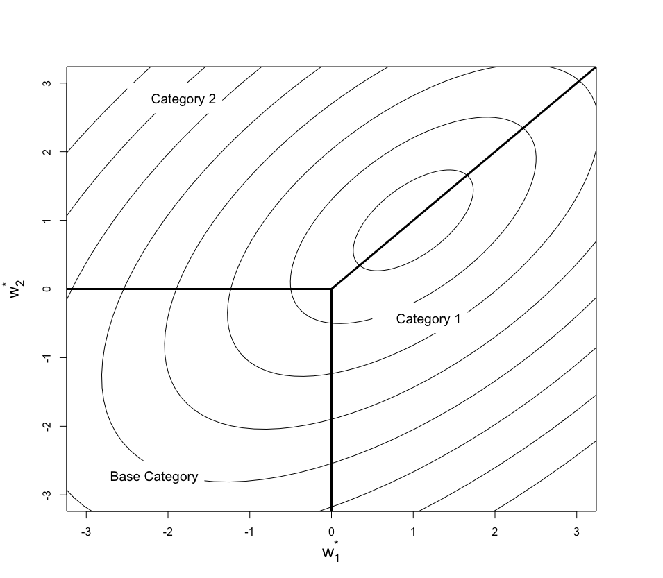
Figure 1: A depiction of the multivariate normal contours associated to the base-subtracted utility space for $p-1=2$. The base category standardization entails that the area in utility space allocated to the base category is a different shape than the regions allocated to non-base categories, meaning that standard priors over $\Sigma^{*}$ (which govern the contours) will result in asymmetric priors on the implied choice probabilities, which correspond to the probability, according to the prescribed multivariate normal distribution, of being in the various sectors associated with each category.

Consider a simple case with $p=3$ categories and focus on one of the three outcome categories, which we will refer to as the “category of interest” (which is fixed). First, we consider a specification where the category of interest is the base category (denoted by $Y_{i}=0$). Then, we consider a specification where the category of interest is the first non-base category (denoted by $Y_{i}=1$).

Our experience indicates that sensitivity to the base category primarily comes from the prior on $\Sigma^{*}$ (rather than $\beta^{*}$), so we will condition on $\beta^{*}$ in order to clarify the issue. Specifically, consider $X_{i}\beta=(v,0,0)$ for an arbitrary value of $v$ and let the first category be the category of interest. Then, if category 1 is the base category, we have $X_{i}^{*}\beta^{*}=(-v,-v)$ corresponding to categories 2 and 3; and when category 2 is the base category we have $X_{i}^{*}\beta^{*}=(v,0)$ corresponding to categories 1 and 3.

Figure 2: The left-hand panel displays prior densities of the probability for the “outcome of interest” when it is coded as the base category (solid) and not the base category (dashed) for a particular value of $\beta$. More precisely, it is the prior density of $\varphi_{j}(1;\Sigma^{*})$ for $j=0,1$, where $j=0$ corresponds to the solid curve, and $j=1$ corresponds to the dashed curve. See expressions (9) – (11) in the main text. The right-hand panel plots $\psi_{j}(v)$ across a range of $v$. That is to say, the average values of the distributions in the left-hand panel correspond to the values in the right-hand panel at $v=1$.

Our interest is in the quantities

$$\varphi_{0}(v;\Sigma^{*}) = \Pr(Y_{i}=0\mid X_{i}^{*}\beta^{*}=(-v,-v)^{\top},\Sigma^{*})$$ (9)

$$\varphi_{1}(v;\Sigma^{*}) = \Pr(Y_{i}=1\mid X_{i}^{*}\beta^{*}=(v,0)^{\top},\Sigma^{*})$$ (10)

$$\psi_{j}(v) = \int\varphi_{j}(v;\Sigma^{*})p(\Sigma^{*})d\Sigma^{*}\quad\mbox{ for }j=0,1.$$ (11)

Note that (9) and (10) both denote the probability that the category of interest is selected, but under different specification of the base category. In (11), $p(\Sigma^{*})$ refers to the trace-restricted variant of the Imai and van Dyk prior for $\Sigma^{*}$ with $\nu=2$ degrees of freedom, and centered at $S=.5J_{2}J_{2}^{\top}+.5I_{2}\propto T_{bc}T_{bc}^{\top}$, with ones on the diagonal.

Figure 2 compares $\varphi_{j}$ and $\psi_{j}$ for $j=0,1$. From the left-hand panel, note that there are strong differences in the range of probabilities for the outcome of interest that are supported by the prior for $\Sigma^{*}$, after conditioning on $\beta^{*}$. In particular, the distribution probabilities for the base category (solid curve) has a very sharp mode, and is less diffuse in general relative to distribution for the nonbase category (dotted curve). On the other hand, the curves in the right-hand figure nearly coincide with one another. This indicates that differences between the two parametrizations in the prior are obscured by marginalizing over the distribution of $\Sigma^{*}$. However, we note that these curves often times do not coincide after conditioning on observed data, as will be shown in Figures 3 and 7.

Because the differences in probabilities appear primarily to be of second and higher moments, an ad-hoc solution to the problem of base category dependence (such as specifying alternative values of the hyperparameters, or by specifying a different $p(\beta^{*}|\Sigma^{*})$ to compensate) may be difficult. Although we expect the impact of the prior to fade as the sample size increases, information in multinomial models accrues slowly relative to standard models of a continuous outcome, which means that asymmetries in the prior for an MNP model may persist in the posterior for sample sizes that are typical in business and economics applications. Hence, we pursue a prior that is identically invariant to relabeling the outcome categories.

2 A symmetric prior for MNP regressions

We now propose a symmetric MNP (sMNP) model that is invariant under relabeling or reordering of the outcome categories. Rather than identifying the locations of the latent utilities by subtracting one from the others, we instead require that they sum to zero. (This assumes that the choice-specific covariates have mean zero for each observation, which is a convenient but inessential standardization.) Further, we assume that the regression parameters that correspond to each agent-specific covariate sum to zero, which gives the same degrees of freedom as the standard MNP, where (in a sense) the regression parameters related to the base category are set equal to zero.

With this sum-to-zero restriction on the utilities, we require a covariance for $W_{i}$ that is symmetric and positive-semidefinite with $p-1$ positive eigenvalues, and constrained in some way in order to set the scale of the model. Rather than directly specifying a distribution on $p\times p$ matrices, we build it up with a mixture of trace-restricted positive-definite matrices. Conditionally, we assume that a positive-definite matrix of dimension $p-1$ describes the covariance of all but one of the dimensions of $W_{i}$. We denote the left-out category with the parameter $b$, and refer to it as the faux base category indicator. In contrast to previous MNP models, $b$ is learned according to Bayes rule.

The proposed model is as follows:

$$b \sim \mbox{unif}(\{1,\ldots,p\})$$ (12)

$$\Sigma_{b} \sim p_{\mbox{\tiny TR}}(S_{b},\nu_{b})$$ (13)

$$R_{b} = [\mbox{chol}(\Sigma_{b})]^{\top}$$ (14)

$$R = \begin{bmatrix}R_{1:(b-1)}\\ R_{b}^{*}\\ R_{b:p}\end{bmatrix}$$ (15)

$$\beta_{b} \sim \mbox{normal}(0,A)$$ (16)

$$\beta = f(\beta_{b})$$ (17)

$$W_{i} \operatorname{\stackrel{{\scriptstyle\mbox{\tiny ind}}}{{\sim}}} \mbox{normal}(X_{i}\beta,RR^{\top})$$ (18)

$$Y_{i} = \operatornamewithlimits{arg\,max}_{j}W_{i}.$$ (19)

Here, $p_{\mbox{\tiny TR}}$ refers to the trace-restricted variant of the Imai and van Dyk (2005a) prior in (7) with $\{\operatorname{tr}(\Sigma_{b})=(p-1)\}$. Its hyperparameters $S_{b}$ and $\nu_{b}$ may change with $b$ but we recommend using common hyperparameters in most cases, since $S_{b}=\operatorname{diag}\{(1+c,\ldots,1+c)\}-cJ_{p-1}J_{p-1}^{\top}$ for all $b$ and a common $\nu_{b}$ will yield a prior covariance structure that is symmetric with respect to the outcome categories. Burgette and Nordheim (2012) discuss tradeoffs for different hyperparameter choices in the trace-restricted prior. Following their guidance, we choose a default value of $\nu_{b}=p+1$. This choice provides sufficient regularization without being too informative. This corresponds to the first $p-1$ rows and columns of a symmetric $p\times p$ covariance matrix $P$ with $p-1$ positive eigenvectors that is symmetric with respect to relabeling the rows and columns. This matrix has the property that vectors drawn from the $\mbox{normal}(0,P)$ distribution sum to zero almost surely, which is a natural center for our relabeling invariant, sum-to-zero MNP. Using $c=0$ means roughly that we expect $p-1$ of the dimensions of the utilities to be independent, with the remaining dimension strongly anti-correlated. We recommend using $c=1/(p-1)$ since it is a more neutral prior and seems to lead to better mixing in the MCMC.

$R_{b}$ is the transposed Cholesky decomposition of $\Sigma_{b}$ such that $R_{b}R_{b}^{\top}=\Sigma_{b}$. $R_{b}^{*}$ is a row vector inserted into $R_{b}$ at the $b$th row such that the sum of each column of $R$ is zero. In this formulation, $\beta_{b}$ has dimension $(p-1)(k_{d}+1)+k_{a}$ (assuming that intercept terms are included in the matrix of covariates as stated in Section 1.2). The function $f$ acts on $\beta_{b}$ such that for each sub-vector of length $p-1$ that corresponds to an agent-specific covariate (or the intercepts), $\beta$ is equal to $\beta_{b}$ with an extra dimension inserted at the $b$th position in the sub-vector. This inserted element is chosen so that the sub-vector sums to zero. With this model specification, we induce a prior distribution on the set of positive-semidefinite matrices of dimension $p$ that have exactly $p-1$ positive eigenvalues.

To make the motivation of this new set of identifying restrictions explicit, we note that they result from transforming the unnormalized utilities not by $T_{\mbox{\tiny bc}}$ as in (3), but rather multiplying them by a $p$-dimensional square matrix $T_{s}$ that is defined to have ones on the main diagonal, and entries of $-1/(p-1)$ elsewhere. Note that $\arg\max W_{i}=\arg\max T_{s}W_{i}$, while the elements of $T_{s}W_{i}$ sum to zero. This transformation also induces the proposed identifying restrictions on $\beta$. If we partition $\beta=(\beta_{d},\beta_{a})$, where $\beta_{a}$ corresponds to the covariates that vary by outcome category, we have

$$T_{s}X_{i}\beta=X_{i}\begin{bmatrix}(I\otimes T_{s})\beta_{d}\\ \beta_{a}\end{bmatrix}.$$ (20)

This transformed version of $\beta$ (i.e., the second factor on the right-hand side of the above equation) conforms to the proposed identifying restrictions. Similarly, a normal distribution with mean zero and covariance $T_{s}\Sigma T^{\top}_{s}$ results in draws that sum to zero almost surely. (Note that $T_{s}$ is almost idempotent in the sense that $T_{s}T_{s}=cT_{s}$ for some scalar $c$. The first $p-1$ rows and columns of $T_{s}$ therefore serve as our default for $S_{b}$ since this corresponds to the transformed variance of $\varepsilon_{i}$ if its variance in the unnormalized scale is proportional to the identity.)

We emphasize that there is nothing inherently wrong with using the asymmetric identifying transformation $T_{\mbox{\tiny bc}}$. If we do not wish for our inferences to depend on the base category, however, the prior must compensate for the asymmetries in the transformation. This seems quite difficult to achieve, especially if we hope to have a computationally tractable model. Using $T_{s}$, however, we can decouple prior specification and model identification, all while preserving the favorable computational characteristics of existing MNP models.

2.1 Model estimation

We propose a Gibbs sampler to estimate the model by constructing a Markov chain on a transformed space: $(\alpha,\Sigma_{b},b,W,\beta_{b})\mapsto(\alpha,\Sigma_{b},b,\tilde{W}=\alpha W,\tilde{\beta}_{b}=\alpha\beta_{b})$. By explicitly working in the $(\alpha,\Sigma_{b},b,\tilde{W},\tilde{\beta}_{b})$ parametrization in specifying the Gibbs sampler we avoid the mistakes discussed in Jiao and van Dyk (2015), although our algorithm is different than theirs.

Remark.

Note that at every iteration in the Markov chain, $\Sigma_{b}$ is restricted to satisfy the identifying trace restriction.

Remark.

For brevity, the notation $\tilde{\Sigma}_{b}$ and $\tilde{\beta}_{b}$ (respectively $\Sigma_{b}$ and $\beta_{b}$) obscures the fact that there are in fact $p$ entities in our parameter space, one for each possible value of $b=1,\dots,p$. However, given $b$ (the “working base category”), this collection of parameters only appears in the likelihood via $\Sigma=g(\Sigma_{1},\dots,\Sigma_{p},b)=RR^{T}$ as defined in (14) and (15) and $\beta=f(\beta_{1},\dots,\beta_{p},b)=f(\beta_{b})$ as in (17). As such, it does little harm to consider only the element of $(\tilde{\Sigma}_{1},\dots,\tilde{\Sigma}_{p})$ and $(\tilde{\beta}_{1},\dots,\tilde{\beta}_{p})$, respectively, $(\Sigma_{1},\dots,\Sigma_{p})$ and $(\beta_{1},\dots,\beta_{p})$, corresponding to the current value of $b$ in the Markov chain.

Let $X_{i,b}$ indicates $X_{i}$ with the $b$th row and the columns specific to the $b$th category removed. We initialize the latent utilities $W_{i}$ by sampling a standard normally-distributed vector of length $p$ and centering it at zero. We then permute its elements so that the maximum of each $W_{i}$ coincides with the observed $Y_{i}$.

The sampler proceeds in three steps:

1. Draw $\tilde{W}\mid Y,\tilde{\beta}_{b},b,\Sigma_{b},\alpha$.

2. Draw $\tilde{\beta}_{b}\mid Y,b,\Sigma_{b},\tilde{W},\alpha$.

3. Draw $\alpha,\Sigma_{b},b\mid Y,\tilde{\beta}_{b},\tilde{W}$.

Note that all variables referenced in these Gibbs steps are from the same parameterization: $(\alpha,\Sigma_{b},b,\tilde{W},\tilde{\beta}_{b})$. We give detailed expressions for each conditional distribution in the appendix. For the draw of the latent utilities $\tilde{W}$, we note that in the original parametrization we have

$$p(W,\alpha\mid\Sigma_{b},\beta_{b},Y,b)\propto I(W,Y)p(W;\beta_{b},\Sigma_{b})p_{TR}(\alpha\mid\Sigma_{b},b).$$

By definition, $\tilde{W}=\alpha W$ and $I(W,Y)$ is the indicator that the utilities and data match correctly, so with $\alpha$ known at this stage of the Gibbs sampler, we write the conditional distribution as:

$$p(\tilde{W}\mid\Sigma_{b},\tilde{\beta}_{b},Y,b,\alpha)\propto I(\tilde{W}/\alpha,Y)p(\tilde{W};\tilde{\beta}_{b},\alpha^{2}\Sigma_{b}).$$

To sample $\tilde{W}$, we iterate one-by-one through the elements of $\tilde{W}_{i,b}$. Note that $\tilde{w}_{i,b}$ is known given $b$ and $\tilde{W}_{i,b}$. After dropping the $b$th element of $\tilde{W}_{i}$ and the corresponding elements in $X_{i}$ and $\beta$, the full conditionals of elements of $\tilde{W}_{i,b}$ are truncated univariate normal. The conditional means and variances can be calculated as described by McCulloch and Rossi (1994), using $\tilde{\beta}_{b}$ as the coefficient vector and $\alpha^{2}\Sigma_{b}$ as the covariance. These truncations are given in the appendix.

The second draw of the transformed coefficients $\tilde{\beta}_{b}$ is from a normal distribution whose conditional mean and variance are provided in the appendix. The third step is a draw of the triplet of parameters $(\alpha,\Sigma_{b},b)$. This is divided into a multinomial draw for $b$ (with the variance integrated out) followed by a draw of an intermediate quantity for the variance, $\tilde{\Sigma}_{b}$. Finally, $\alpha$ and $\Sigma_{b}$ are obtained by first setting $\alpha=\sqrt{\operatorname{tr}(\tilde{\Sigma}_{b})/(p-1)}$, followed by $\Sigma_{b}=\tilde{\Sigma}_{b}/\alpha^{2}$. In this way, $\operatorname{tr}(\Sigma_{b})=p-1$ at each iteration as in Burgette and Nordheim (2012).

Having obtained samples from the Markov chain defined over $(\alpha,\Sigma_{b},b,\tilde{W},\tilde{\beta}_{b})$, one can transform, per-iteration, back to the original space to obtain samples of $W=\tilde{W}/\alpha$ and $\beta_{b}=\tilde{\beta}_{b}/\alpha$. In the following section, we demonstrate this methodology on two consumer choice data sets as well as investigate its properties with a simulation study.

3 Demonstrations

3.1 Clothes detergent purchases

Imai and van Dyk (2005a, b) apply their methods to a consumer choice model of clothing detergent purchases. The data are available in their MNP package in R. We have records of purchasing decisions along with available log-prices for shoppers choosing between All, Era Plus, Solo, Surf, Tide, and Wisk brand detergents. There are 2657 observations and only six regression parameters, so we typically do not see large differences in estimated purchase probabilities based on the various base category fits. However, specifying the base category to be All — which is rarely purchased despite its low price — does give somewhat different predictions for All when its price is low. We see this in Figure 3, where we set the prices for all other brands at their brand-specific average, and consider predicted purchase probabilities across a range of low prices for All. The predictions from five of the base categories (solid curves) are very similar. The predictions when All is the base category (dashed curve) are notably higher. When we apply the sMNP to the data, we see that its predictions are intermediate to those of the various base category fits (dotted curve). In each case, the estimated purchase probability is routinely computed from the posterior predictive distribution.

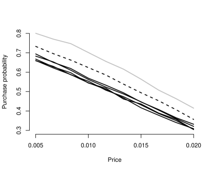
Figure 3: Estimated purchase probabilities for All brand detergent, with all other brands’ prices fixed at the brand-specific mean observed price. The dashed curve uses All as the base category; the solid curves use all of the other possible base categories. The dotted curve results from an sMNP fit. Although the model is fit as a function of log-price, we display results as a function of dollars.

To interpret the $\beta$ parameters, we know — by the sum-to-zero property of the intercept terms — that a brand with an intercept coefficient that is persistently negative (All) is less desirable than average, in a sense (Figure 4). EraPlus and Tide are estimated to be more desirable. However, note that these intercepts do not reflect marginal purchase probabilities, as less desirable brands may also have lower prices. As economic theory would suggest, the price coefficient is strongly negative (Figure 5), which indicates that raising a detergent’s price (relative to the competitors) will lower its estimated purchase probability.

Although these interpretations of the $\beta$ parameters are accurate, we would argue that summaries of MNP results are best phrased in terms of changes in posterior predicted selection probabilities. For example, one might consider the effect of a proposed price increase on the current purchase probabilities. We advocate this because predictions take into account both $\beta$ and $\Sigma$ parameters, and the $\Sigma$ parameters can be very difficult to interpret on their own. If only the $\beta$ parameters are of interest in an application, we would argue that a model that assumes IIA may be more appropriate.

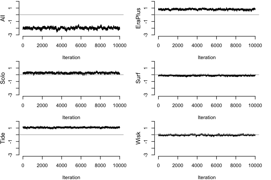
Figure 4: Trace plots of samples from the posterior distributions of the intercept terms for an sMNP fit of the detergent data.

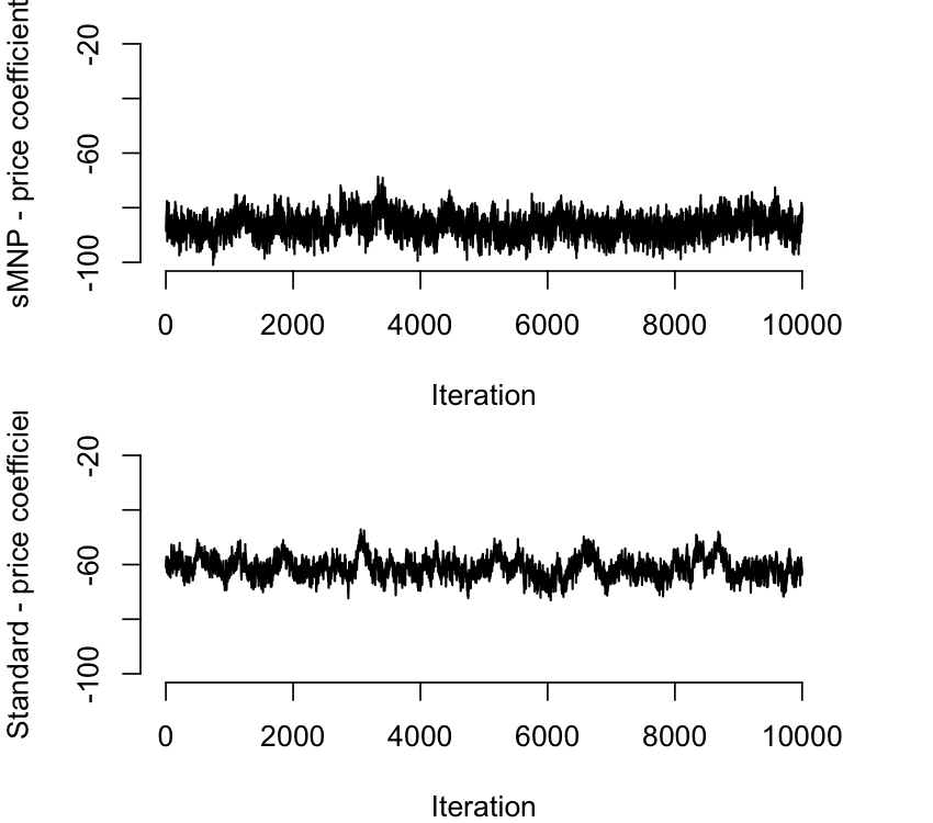
Figure 5: Trace plots of samples from the posterior distributions of the price coefficients for sMNP and standard MNP fits of the detergent data.

We also highlight the mixing behavior of the sMNP algorithm. For example, the faux base parameter $b$ mixes extremely well, as indicated by the near constant switching between its six possible values (Figure 6). Further, the mixing of the price parameter in the symmetric MNP algorithm compares favorably to the base category MNP in fits of these data (Figure 5). Imai and van Dyk (2005a) used these data to demonstrate improved mixing performance of their model relative to earlier MNP models, so these results are a comparison against the state of the art.

Here, the posterior of $b$ remains relatively flat. However, the extent that the data are informative about $b$ is precisely because the prior, for any fixed $b$, remains asymmetric. Consequently, in any finite data set, one of the base categories will look slightly “better” by the light of the prior predictive distribution for some particular base category. The fact that the data can inform us about $b$ is precisely why including $b$ in the model is necessary. Fixing $b$ at some arbitrary value, rather than moving the posterior probability of the “faux bases”, would instead influence posterior inferences concerning the parameters of interest, such as choice probabilities themselves. Consequently, as a practical matter we do not recommend reporting posterior inferences on $b$, as they are a mere device for specifying a symmetric prior.

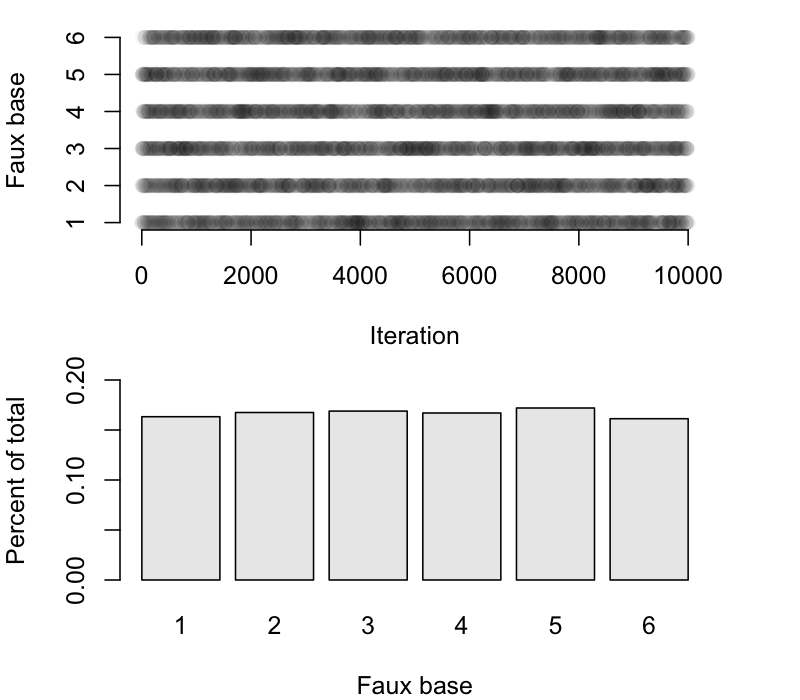
Figure 6: Trace plot and histogram of samples from the posterior distribution of faux base parameters $b$ for the detergent data. In the upper panel, points are plotted with 2% intensity. The numbers 1 through 6 correspond to All, EraPlus, Solo, Surf, Tide, and Wisk, respectively.

3.2 Margarine purchases

We also consider a similar analysis of consumer purchases of margarine that are available in the bayesm package in R. Again, our model only has intercepts and a price coefficient. Following McCulloch and Rossi (1994), we limit our analysis to purchases of Parkay, Blue Bonnet, Fleischmann’s, House brand, Generic, and Shedd Spread tub margarines. And, following Burgette and Nordheim (2012), we limit the analysis to the first purchase of one of these brands for each household. This results in a dataset with 507 observations. With the smaller sample size, there are larger differences in posterior estimated purchase probabilities when one switches from one base category to another in standard MNP fits.

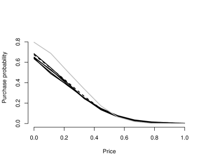
Figure 7: Estimated purchase probabilities for House brand margarine over a range of prices for that brand, with other prices fixed. The solid curves are posterior predictions from standard MNP models, and the dashed curve is from the sMNP. The gray curve uses House brand as the base category.

In Figure 7, we see that sMNP predictions again tend to be between those of standard MNP models when we consider all possible base categories, as was the case in Figure 3. The observed House brand prices are between $0.19 and $0.64, so there is significant disagreement across nearly the entire range of observed prices for that brand. (With the larger sample size in the detergent data, we only saw meaningful differences when we extrapolated out of the observed price range.) Although there is some Monte Carlo error in the estimates, it is insignificant compared to the 19% difference between the low and high estimates of House’s selection probability when it is priced at $0.20.

Thus, in both of these examples, we see that the sMNP gives predictions that are between those of the standard MNP models that are fit alternately with each base. This is compatible with the heuristic interpretation of the sMNP as a model that averages across base categories in standard MNP models.

An alternative approach to handling dependence on the base category would be to fit an Imai and van Dyk-style MNP model using each base category separately, and perform a post-hoc average of the fitted probabilities. We find this to be unappealing from several perspectives. First, the computation load is $p$ times as large as it would be for a single, standard MNP fit; the sMNP is only slightly more expensive than a single base category MNP. More importantly, the sMNP constitutes a proper Bayesian procedure, which automatically incorporates posterior uncertainty about the base category and uses a likelihood-weighted average of the possible models (bottom panel of Figure 6).

3.3 A simulation study

Here we compare the fitted probabilities of MNP models that use each of the possible base categories and the fitted probabilities that result from the base category-free sMNP. We simulate 50 datasets that are loosely based on the consumer choice examples above. We assume that $n=750$ consumers are choosing from $p=6$ products. The simulated product-specific intercepts and mean prices have correlation $0.9$ so that more desirable products are more expensive, as one would expect. The price coefficient was drawn uniformly from $[-1.25,-.75]$ so that if a product is relatively less expensive, it will be more popular. Finally, a $p\times p$ covariance matrix with expectation $I$ is drawn from an inverse-Wishart distribution with 50 degrees of freedom. The simulation parameters were chosen so that each “brand” is chosen with high probability. Note that the data parameters were chosen without regard to any set of identifying restrictions.

We measure performance via the total variation between the estimated and true purchase probabilities, averaged over the first 10 sets of prices in each simulated dataset. We expect that the sMNP will be less prone to making “extreme” predictions in the sense of Figure 7. The results are summarized in Figure 8, and are consistent with this notion. The plot gives the average total variation from the true purchase probabilities for each of the base category MNP models (hollow circles) and the sMNP (solid circles). Note that the sMNP is never the worst among the various base category models. In 18 of the 50 simulated cases, sMNP outperformed all of the base category models. In 41 out of 50 of the simulations, the sMNP performed better than the median base category performance.

Figure 8: Simulation results. Points give the average percent total variation between true and estimated purchase probabilities. Solid black circles are from the sMNP. Hollow gray circles are from MNP models that use each of the six possible base category identifying restrictions. The sMNP is almost never worse than every base category model, only 1 out of 50 cases, and in 41 out of 50 cases it beats the median performing base category.

4 Identification

A potential downside to our model is that it is not formally identified. In particular, the model would be identified if we were able to restrict the trace of $\Sigma$, rather than the trace of $\Sigma_{b}$. If one of the diagonal elements of $\Sigma$ is estimated to be substantially larger than 1, then the scale of $\beta$ will depend on $b$. Although a fully identified model may be preferable, we argue that little is lost in this case.

First — from the perspective of prior specification/elicitiation — the model is identified conditional on the discrete parameter $b$. If the analyst wishes to specify an informative prior, this can be done conditionally for each $b=1,\ldots,p$. If the model were only identified conditional on a continuous working parameter, this process becomes more difficult. Second — on the side of interpretation — we would argue that $\beta$ parameters should be interpreted while taking $\Sigma$ into account, and vice versa. Since marginal summaries do not do this, we feel that the best model summaries are changes of fitted probabilities as a function of key outcome variables such as in Figure 7, which are not impacted by this identification issue. If the analyst truly is interested in features of the marginal posterior distribution of $\beta$ or $\Sigma$, it is possible to post-process the results into a single, identified scale by re-scaling the sampled values at each iteration of the MCMC such that, for example, the trace of $\Sigma$ is equal to $p$. However, the signs of the estimated $\beta$ parameters are not impacted by the under-identification of our model.

Post-processing in order to identify Bayesian MNP models was popularized by McCulloch et al. (2000), in the context of specifying a prior for $\tilde{\Sigma}^{*}$, rather than the identified $\Sigma^{*}$. As an aside, we note that a related idea for solving the base category problem would be to specify a full-rank inverse-Wishart prior for $\Sigma$, without worrying about the conditional identifying restriction on the location of the $W_{i}$. However, this approach proves to be numerically unusable. The $p$-dimensional inverse-Wishart prior pushes the sampled values of $\Sigma$ toward the edge of the parameter space, which quickly results in numerical problems that result from sampling poorly-conditioned covariance matrices.

5 Conclusion

The analyses in this paper demonstrate that careful handling of the prior is necessary in order to obtain reliable predictions from the Bayesian MNP. As with any proper Bayesian model, our estimates are biased, but they are not biased against any particular outcome category in the prior. The same can not be said of previous MNP models that estimate the covariance of the utilities.

With the prior for the regression coefficients centered on zero, the sMNP estimates should be pulled toward more moderate estimates. Since multinomial data are quite coarse (in the sense that each observation contributes little information compared to a multivariate normal regression where the utilities are observed) we would argue that this prior-induced regularization toward moderate predictions is highly desirable.

When building more advanced MNP models, symmetry may take on even greater importance. For example, Cripps et al. (2010) proposed an MNP model that allows for a sparse representation of the precision matrix of the latent utilities. However, they induce sparsity in the precision of the base-subtracted utilities, not in the precision of the original utilities. This seems very likely to exacerbate the problem of posterior estimates changing across different specifications of the base category. Further, it is unclear that sparsity in the base-subtracted precision corresponds to a meaningful data-generating process. That said, it is likely that favorable bias/variance tradeoffs can be made by specifying a prior that pulls the precision toward a well-chosen, sparse structure.

More broadly, the regularizing effect of a Bayesian prior distribution is at its most powerful when the likelihood is poorly behaved in some way: when it is flat or spiky; when identification is weak; when the number of parameters is large relative to the sample size. However, in each of these situations, we should be worried that if our prior has undesirable features, they may be preserved in the posterior. For example, MNP likelihoods can be quite flat, and therefore the asymmetry of previously-proposed priors can propagate to the posterior. Data analysts may hope that such undesirable features of the prior would be overwhelmed by the likelihood. This research suggests that while we cannot always count on the data to cover flaws of our priors, we may be able to design priors that lack the flaw in the first place, without giving up computational tractability.

Appendix

Full conditional distributions for the Gibbs sampler

In the following sections, we provide expressions for the conditional distributions used in the Gibbs sampler. The full conditionals that are standard distributions are determined by extracting relevant components from the joint distribution of all parameters. The means and variances for the truncated univariate normal distributions follow from McCulloch and Rossi (1994).

Step 1: Draw $\tilde{W}\mid Y,\tilde{\beta}_{b},b,\Sigma_{b},\alpha$

To sample $\tilde{W}$, we iterate one-by-one through the elements of $\tilde{W}_{i,b}$. Note that $\tilde{w}_{i,b}$ is known given $b$ and $\tilde{W}_{i,b}$. After dropping the $b$th element of $\tilde{W}_{i}$ and the corresponding elements in $X_{i}$ and $\beta$, the full conditionals of elements of $\tilde{W}_{i,b}$ are truncated univariate normal. The conditional means and variances can be calculated as described by McCulloch and Rossi (1994), using $\tilde{\beta}_{b}$ as the coefficient vector and $\alpha^{2}\Sigma_{b}$ as the covariance. The truncations are:

• If $Y_{i}=j\neq b$, sample $\tilde{w}_{ij}$ from a truncated normal so that $\tilde{w}_{ij}>-.5\sum_{k\notin\{j,b\}}\tilde{w}_{ik}$ and $\tilde{w}_{ij}>\max(\tilde{w}_{ik}:k\notin\{j,b\})$.

• If $Y_{i}\neq b$ and $Y_{i}=k\neq j$, sample $w^{\star}_{ij}$ from a truncated normal so that $\tilde{w}_{ij}<\tilde{w}_{ik}$ and $\tilde{w}_{ij}>-\sum_{l\neq b}\tilde{w}_{il}-\tilde{w}_{ik}$.

• If $Y_{i}=b$, sample $\tilde{w}_{ij}$ from a truncated univariate normal such that

  $$\tilde{w}_{ij}<\min\{-.5\sum_{k\not\in\{b,j\}}\tilde{w}_{ik},-1(\max\{\tilde{W}_{-\{j,b\}}\}+\sum_{k\not\in\{b,j\}}\tilde{w}_{ik})\}.$$

Step 2: Draw $\tilde{\beta}_{b}\mid Y,b,\Sigma_{b},\tilde{W},\alpha$

The transformed coefficient vector is drawn according to a normal distribution. This arises from the normal likelihood coupled with the normal prior specified for the coefficient vector, and standard Bayesian linear regression analysis specifies the conditional moments in closed form. They are as follows:

$$\hat{\beta}_{b} = [\sum_{i=1}^{n}X_{i,b}^{\top}\Sigma_{b}^{-1}X_{i,b}+A^{-1}]^{-1}[\sum_{i=1}^{n}X_{i,b}^{\top}\Sigma_{b}^{-1}\tilde{W}_{i,b}],$$

$$\tilde{\beta}_{b} \sim \mbox{normal}\bigg{(}\hat{\beta}_{b},\alpha^{2}\big{(}\sum_{i=1}^{n}X_{i,b}^{\top}\Sigma_{b}^{-1}X_{i,b}+A^{-1}\big{)}^{-1}\bigg{)}.$$

This update follows from the fact that if $\beta_{b}\sim\mbox{normal}(0,A)$, then $\tilde{\beta}_{b}\sim\mbox{normal}(0,\alpha^{2}A)$.

Step 3: Draw $\alpha,\Sigma_{b},b\mid Y,\tilde{\beta}_{b},\tilde{W}$

The draw from this distribution is divided into a couple steps. First, draw $b\mid\tilde{\beta},\tilde{W}$. Second, by working with the intermediate quantity $\tilde{\Sigma}_{b}$, draw $\tilde{\Sigma}_{b}\mid b,\tilde{\beta},\tilde{W}$. Once obtained, set $\alpha=\sqrt{\operatorname{tr}(\tilde{\Sigma}_{b})/(p-1)}$, followed by $\Sigma_{b}=\tilde{\Sigma}_{b}/\alpha^{2}$. In this way, $\operatorname{tr}(\Sigma_{b})=p-1$ at each iteration as in Burgette and Nordheim (2012).

Computationally, the major change from Burgette and Nordheim (2012) is the draw from $(b,\tilde{\Sigma}_{b})$. We derive this draw by first noting that from the full conditional we have:

$$p(b,\tilde{\Sigma}_{b}|\mbox{all}) \propto \exp\{-.5\sum(\tilde{W}_{i,b}-X_{i,b}\tilde{\beta}_{b})^{\top}\tilde{\Sigma}_{b}^{-1}(\tilde{W}_{i,b}-X_{i,b}\tilde{\beta}_{b})\}$$

$$\times|\tilde{\Sigma}_{b}|^{-n/2}p(\tilde{\Sigma}_{b}|b)p(b)$$

$$\propto \exp\{-.5\operatorname{tr}(\tilde{\Sigma}^{-1}(S_{b}+\sum(\tilde{W}_{i,b}-X_{i,b}\tilde{\beta}_{b})(\tilde{W}_{i,b}-X_{i,b}\tilde{\beta}_{b})^{\top}))\}$$

$$\times|\tilde{\Sigma}_{b}|^{-.5(n+\nu_{0}+p)}.$$

Integrating over the variance, we obtain the multinomial draw for $b$ as:

$$p(b|\tilde{\beta},\tilde{W}) \propto \int p(b,\tilde{\Sigma}_{b}|\mbox{all})d\tilde{\Sigma}_{b}$$

$$\propto |S_{b}+\sum(\tilde{W}_{i,b}-X_{i,b}\tilde{\beta}_{b})(\tilde{W}_{i,b}-X_{i,b}\tilde{\beta}_{b})^{\top}|^{-(n+\nu_{b})/2}$$

Then, conditional on $b$, $\tilde{\Sigma}_{b}$ can be sampled from an inverse-Wishart distribution as shown in the full conditional above and described by Imai and van Dyk (2005a).

References

- (1)
- Albert and Chib (1993) Albert, J., and Chib, S. (1993), “Bayesian analysis of binary and polychotomous response data,” Journal of the American Statistical Association, 88(422), 669–679.
- Burgette and Nordheim (2012) Burgette, L., and Nordheim, E. (2012), “The trace restriction: An alternative identification strategy for the Bayesian multinomial probit model,” Journal of Business and Economic Statistics, 30(3), 404–410.
- Cripps et al. (2010) Cripps, E., Fiebig, D., and Kohn, R. (2010), “Parsimonious estimation of the covariance matrix in multinomial probit models,” Econometric Reviews, 29(2), 146–157.
- Fong et al. (2016) Fong, D. K., Kim, S., Chen, Z., and DeSarbo, W. S. (2016), “A Bayesian multinomial probit model for the analysis of panel choice data,” Psychometrika, 81(1), 161–183.
- Garrido and Mahmassani (2000) Garrido, R., and Mahmassani, H. (2000), “Forecasting freight transportation demand with the space-time multinomial probit model,” Transportation Research Part B: Methodological, 34(5), 403–418.
- Hoff (2009) Hoff, P. (2009), “Simulation of the Matrix Bingham–von Mises–Fisher distribution, with applications to multivariate and relational data,” Journal of Computational and Graphical Statistics, 18(2), 438–456.
- Imai and van Dyk (2005a) Imai, K., and van Dyk, D. (2005a), “A Bayesian analysis of the multinomial probit model using marginal data augmentation,” Journal of Econometrics, 124(2), 311–334.
- Imai and van Dyk (2005b) Imai, K., and van Dyk, D. (2005b), “MNP: R package for fitting the multinomial probit model,” Journal of Statistical Software, 14(3), 1–32.
- Jiao and van Dyk (2015) Jiao, X., and van Dyk, D. A. (2015), “A corrected and more efficient suite of MCMC samplers for the multinomal probit model,” arXiv preprint arXiv:1504.07823, .
- McCulloch et al. (2000) McCulloch, R., Polson, N., and Rossi, P. (2000), “A Bayesian analysis of the multinomial probit model with fully identified parameters,” Journal of Econometrics, 99(1), 173–193.
- McCulloch and Rossi (1994) McCulloch, R., and Rossi, P. (1994), “An exact likelihood analysis of the multinomial probit model,” Journal of Econometrics, 64(1), 207–240.
- McFadden (1974) McFadden, D. (1974), “The measurement of urban travel demand,” Journal of Public Economics, 3(4), 303–328.
- Rossi et al. (2005) Rossi, P., Allenby, G., and McCulloch, R. (2005), Bayesian Statistics and Marketing, Chichester, West Sussex, England: Wiley.
- Rudolph (2003) Rudolph, T. (2003), “Who’s responsible for the economy? The formation and consequences of responsibility attributions,” American Journal of Political Science, 47(4), 698–713.
- Tanner and Wong (1987) Tanner, M., and Wong, W. (1987), “The calculation of posterior distributions by data augmentation,” Journal of the American Statistical Association, 82(398), 528–540.
- Train (2003) Train, K. (2003), Discrete Choice Methods with Simulation, Cambridge: Cambridge University Press.