A high-order discontinuous Galerkin pressure robust splitting scheme for incompressible flows
Dedicated to Mary F. Wheeler in honour of her 80th birthday

Abstract

The accurate numerical simulation of high Reynolds number incompressible flows is a challenging topic in computational fluid dynamics. Classical inf-sup stable methods like the Taylor-Hood element or only $L^{2}$-conforming discontinuous Galerkin (DG) methods relax the divergence constraint in the variational formulation. However, unlike divergence-free methods, this relaxation leads to a pressure-dependent contribution in the velocity error which is proportional to the inverse of the viscosity, thus resulting in methods that lack pressure robustness and have difficulties in preserving structures at high Reynolds numbers. The present paper addresses the discretization of the incompressible Navier-Stokes equations with high-order DG methods in the framework of projection methods. The major focus in this article is threefold: i) We present a novel postprocessing technique in the projection step of the splitting scheme that reconstructs the Helmholtz flux in $H(\text{div})$. In contrast to the previously introduced $H(\text{div})$ postprocessing technique, the resulting velocity field is pointwise divergence-free in addition to satisfying the discrete continuity equation. ii) Based on this Helmholtz flux $H(\text{div})$ reconstruction, we obtain a high order in space, pressure robust splitting scheme as numerical experiments in this paper demonstrate. iii) With this pressure robust splitting scheme, we demonstrate that a robust DG method for underresolved turbulent incompressible flows can be realized.

1 Introduction

Navier-Stokes fluid flow at high Reynolds numbers plays an increasing role also for the detailled understanding of subsurface flow processes. Our original interest was in contributing to the understanding of the surface renewal effect at the interface of subsurface and atmosphere [1, 2] which is attributed to coherent turbulent structures interacting with the atmospheric boundary layer at the surface. Other applications include Navier-Stokes flow in rock fractures [3, 4], flow in wellbores [5] as well as flows on the pore-scale [6, 7].

The numerical simulation of flows at high Reynolds numbers is still a challenging task. Most classical finite element methods relax the divergence constraint and only enforce the condition weakly. Recently, it has been understood that the relaxation of the incompressibility constraint introduces a pressure-dependent contribution in the velocity error for inf-sup stable methods like the Taylor-Hood element or only $L^{2}$-conforming DG methods. This insight has led to distinguish between pressure robust and non pressure robust space discretizations, respectively, where a method is called pressure robust if the velocity error is independent of the continuous pressure. The study of pressure robust methods is a current, active research topic [8, 9, 10, 11, 12]. It is connected to the Helmholtz decomposition of vector fields and consequently, a fundamental invariance property of the incompressible Navier-Stokes equations if the boundary conditions do not depend on the pressure: Let $(v,p)$ be the solution of the equations with right-hand side $f$, then a transformation of the body force $f\mapsto f+\nabla\psi$ changes the Navier-Stokes solution $(v,p)\mapsto(v,p+\psi)$, i.e. the velocity field does not change and the additional forcing is balanced by the pressure gradient. A desirable property of a discretization scheme is to maintain an unchanged velocity field under such irrotational force translation. As a simple example let us consider the stationary Stokes equations

$$-\nu\Delta v+\nabla p =f\hskip 8.99994pt\textup{in}\;\Omega$$

$$\nabla\cdot v =0\quad\textup{in}\;\Omega$$

$$v =g\quad\textup{on}\;\partial\Omega$$

$$\int_{\Omega}p\mathrm{d}x =0\;.$$

Employing a $k$-th order mixed finite element DG discretization, the following error estimate in [13, 14] was shown:

$$\bigl{[}\!\|v-v_{h}\|\!\bigr{]}\leq Ch^{k}\left(|v|_{k+1}+\frac{1}{\nu}|p|_{k}\right)$$ (1)

with constant $C$ independent on $h$ and $\nu$, and with the mesh-dependent norm $\bigl{[}\!\|\cdot\|\!\bigr{]}$ for the Stokes problem. The right-hand side in the a-priori estimate (1) is a standard bound for classical mixed finite element methods. Observe that the velocity error depends on the pressure scaled by the inverse of viscosity. This has the consequence that the velocity approximation is not robust with respect to irrotational force translations that would solely change the pressure in the continuous case and therefore this method is not pressure robust. In fact, a consistency error is hidden in the discrete Helmholtz projector such that discretely divergence-free functions need not be $L^{2}$-orthogonal to the irrotational fields. The consistency error is reflected in the pressure term $\frac{1}{\nu}\left|p\right|_{k}$ and renders such space discretizations inaccurate at handling correctly large irrotational parts in a flow, or preserving flow structures, for high Reynolds numbers, especially in an underresolved turbulence computation. In contrast, the pressure-dependent term on the right-hand side disappears if a divergence-free method is employed.

It is thus important for a space discretization to preserve physical properties at the discrete level. To name only a few, inf-sup stable divergence-free mixed methods [15], inf-sup stable $H(\text{div})$ conforming DG methods [16, 17], inf-sup stable finite element methods with appropriately modified velocity test functions [18, 19, 20, 21, 22, 23], and inf-sup stable $L^{2}$-conforming DG methods with additional consistent stabilization terms [24, 25] have been found lately in order to realize this.

High-order DG methods are increasingly important for a wide range of applications including computational fluid dynamics given recent development in modern computer architectures. Their block structure, compact stencils, and high ratio of computation to communication make them well-suited on modern, many-core, memory-constrained architectures. To this extent, there has been recent work on high-order DG methods for the incompressible Navier-Stokes equations, see e.g. [26, 27] for coupled solution approaches, [28], and [24, 29, 30] for discretizations using projection methods. In [28] we have presented a postprocessing technique in the Helmholtz projection step based on $H(\text{div})$ reconstruction of the pressure correction. The obtained velocity field has been shown to satisfy the discrete continuity equation so that the procedure defines a discrete projection operator.

Extending this solution approach, we present in this work a novel postprocessing technique that reconstructs the Helmholtz flux $w_{h}-\nabla_{h}\psi_{h}$ in the Raviart-Thomas space where $w_{h}$ denotes the tentative velocity and $\nabla_{h}\psi_{h}$ is the irrotational correction. The resulting velocity field satisfies the discrete continuity equation, and is also pointwise divergence-free, the latter property not being satisfied by the previously introduced $H(\text{div})$ postprocessing technique. The reconstruction picks up the notion of a divergence-preserving reconstruction operator for discontinuous velocity and pressure ansatz spaces. As numerical experiments demonstrate, exactly the improvement on the pointwise divergence renders the approach to be pressure robust like a divergence-free mixed method. We thereby substantiate the recently made statement [8] that the need for pressure robustness emanates from an improved understanding of mixed methods and the divergence constraint in incompressible flows.

Outline

The article is organized as follows: In Section 2 we introduce the notation for the discontinuous Galerkin formulation and describe the DG discretization of the incompressible Navier-Stokes equations. In Section 3 we introduce splitting methods where we concentrate on the pressure correction scheme in rotational form (RIPCS) throughout this work. Then, several variants of discrete Helmholtz decompositions in the framework of projection methods are reviewed and later compared in the numerical experiments. In Section 4 we present the novel postprocessing technique in the projection step of the splitting scheme that reconstructs the Helmholtz flux $w_{h}-\nabla_{h}\psi_{h}$ in $H(\text{div})$. It is shown that the resulting velocity field satisfies the discrete continuity equation and is pointwise divergence-free. We assess the numerical conservation properties and temporal convergence of the obtained splitting scheme by benchmarks that have been used in a previous publication [28]. In Section 5 the aforementioned variants of discrete Helmholtz decomposition are tested and compared within the pressure correction scheme. The numerical examples include the time-dependent Stokes equations and vortex-dominated flows for small viscosities, and the Beltrami flow. The tests serve to verify pressure robustness and the ability of the methods to preserve structures. Furthermore, the 3D Taylor-Green vortex is utilized as a working horse to demonstrate that with a pressure robust DG method, a robust method for underresolved turbulent incompressible flows can be realized. At the end we conclude in Section 6.

2 Discontinuous Galerkin spatial discretization

The instationary incompressible Navier-Stokes equations in an open and bounded domain $\Omega\subset\mathbb{R}^{d}$ ($d=2,3$) and time interval $(0,T]$ with velocity $v$ and pressure $p$ as unknowns for given right-hand side $f$, viscosity $\mu$ and density $\rho$ are given by

$$\rho\partial_{t}v-\mu\Delta v+\rho(v\cdot\nabla)v+\nabla p =f \textup{in}\;\Omega\times(0,T]$$ (2a)

$$\nabla\cdot v =0 \textup{in}\;\Omega\times(0,T]$$ (2b)

$$v =v_{0} \textup{for}\;t=0\;.$$ (2c)

Either Dirichlet boundary condition for the velocity:

$$v =g \textup{on}\;\Gamma_{D},t\in(0,T]$$ (2d)

and free-slip boundary condition in addition if $$\Gamma_{D}\neq\partial\Omega$$:

$$v\cdot n=0\quad\textup{and}\quad\mu\nabla vn\times n =0 \textup{on}\;\Gamma_{S}=\partial\Omega\setminus\Gamma_{D},t\in(0,T]$$ (2e)

together with

$$\int_{\Omega}p\mathrm{d}x =0 \textup{for all}\;t\in(0,T]$$ (2f)

or mixed boundary conditions:

$$v =g \textup{on}\;\Gamma_{D}\neq\{\partial\Omega,\emptyset\}$$ (2g)

$$v\cdot n=0\quad\textup{and}\quad\mu\nabla vn\times n =0 \textup{on}\;\Gamma_{S}\;\textup{disjoint to}\;\Gamma_{D}$$ (2h)

$$\mu\nabla vn-pn-\rho\beta(v\cdot n)_{-}v =0 \textup{on}\;\Gamma_{N}=\partial\Omega\setminus(\Gamma_{D}\cup\Gamma_{S})$$ (2i)

are supplemented with the system. For pure Dirichlet boundary conditions $g$ is required to satisfy the compatibility condition $\int_{\partial\Omega}g\cdot n\mathrm{d}s=0$ and in addition of free-slip boundary conditions $\int_{\Gamma_{D}}g\cdot n\mathrm{d}s=0$. On $\Gamma_{N}$, $(v\cdot n)_{-}=\min(0,v\cdot n)$ denotes the negative part of the flux across the boundary. The parameter $\beta$ can take the values $\beta=0$ (classical do-nothing, CDN) or $\beta=\frac{1}{2}$ (directional do-nothing, DDN), [31]. In the numerical examples below we will also consider periodic boundary conditions in addition. Under appropriate assumptions the Navier-Stokes problem in weak form has a solution in $(H^{1}(\Omega))^{d}\times L^{2}(\Omega)$ for $t\in(0,T]$, [32, 33]. In absence of do-nothing conditions the pressure is only determined up to a constant and is in the space $L^{2}_{0}(\Omega)=\{q\in L^{2}(\Omega)\mid\int_{\Omega}q\mathrm{d}x=0\}$.

For the discretization let $\mathcal{E}_{h}$ be a quadrilateral mesh (in dimension $d=2$) or a hexahedral mesh (in dimension $d=3$) with maximum diameter $h$. We denote by $\Gamma_{h}^{\mathrm{int}}$ the set of all interior faces, by $\Gamma_{h}^{D}$ the set of all faces intersecting with the Dirichlet boundary $\Gamma_{D}$, by $\Gamma_{h}^{S}$ the set of all faces intersecting with the free-slip boundary and by $\Gamma_{h}^{N}$ the set of all faces intersecting with the mixed boundary $\Gamma_{h}^{N}$. We set $\Gamma_{h}=\Gamma_{h}^{\mathrm{int}}\cup\Gamma_{h}^{D}\cup\Gamma_{h}^{S}\cup\Gamma_{h}^{N}$. To an interior face $e\in\Gamma_{h}^{\mathrm{int}}$ shared by elements $E_{e}^{1}$ and $E_{e}^{2}$ we define an orientation by its unit normal vector $n_{e}$ pointing from $E_{e}^{1}$ to $E_{e}^{2}$. The jump and average of a scalar-valued function $\phi$ on a face is then defined by

$$[\phi] =\phi\mid_{E_{e}^{1}}-\phi\mid_{E_{e}^{2}}\quad\;=\phi^{\mathrm{int}}-\phi^{\mathrm{ext}},$$ (3)

$$\{\phi\} =\frac{1}{2}\phi\mid_{E_{e}^{1}}+\frac{1}{2}\phi\mid_{E_{e}^{2}}=\frac{1}{2}\phi^{\mathrm{int}}+\frac{1}{2}\phi^{\mathrm{ext}}\;.$$

Note that the definition of jump and average can be extended in a natural way to vector and matrix-valued functions. If $e\in\partial\Omega$ then $n_{e}$ corresponds to the outer normal vector $n$. Below we make heavy use of the identities and notation, respectively:

$$[uv] =[u]\{v\}+\{u\}[v]\;, (u,v)_{0,\omega} =\int_{\omega}uv\,\mathrm{d}x\;, u,v$$ ( scalar-valued) (4)

$$[u\cdot v] =[u]\cdot\{v\}+\{u\}\cdot[v]\;, (u,v)_{0,\omega} =\int_{\omega}u\cdot v\,\mathrm{d}x\;, u,v$$ ( vector-valued)

$$[u:v] =[u]:\{v\}+\{u\}:[v]\;, (u,v)_{0,\omega} =\int_{\omega}u:v\,\mathrm{d}x\;, \text{($u,v$ matrix-valued)}.$$

where $\omega\subset\Omega$ is a $d$-dimensional subset together with the $d$-dimensional measure $\mathrm{d}x$. The same shorthand notation holds for the hypersurface measure $\mathrm{d}s$ when integrating over codimension one subsets as (parts of) the boundary or possible collection of faces. The DG discretization on hexahedral meshes is based on the non-conforming finite element space of polynomial degree $p$

$$Q_{h}^{p}=\{v\in L^{2}(\Omega)\mid v|_{E}=q\circ\mu_{E}^{-1},q\in\mathbb{Q}_{p,d},E\in\mathcal{E}_{h}\}$$ (5)

where $\mu_{E}:\hat{E}\to E$ is the transformation from the reference cube $\hat{E}$ to $E$ and $\mathbb{Q}_{p,d}$ is the set of polynomials of maximum degree $p$ in $d$ variables. The approximation spaces for velocity and pressure are then

$$X^{p}_{h}\times M_{h}^{p-1} =(Q_{h}^{p})^{d}\times(Q_{h}^{p-1}\cap L^{2}_{0}(\Omega)) \text{(Dirichlet b. c.)},$$ (6a)

$$X^{p}_{h}\times M_{h}^{p-1} =(Q_{h}^{p})^{d}\times Q_{h}^{p-1} \text{(mixed b. c.)}.$$ (6b)

We make use of the following mesh-dependent forms defined on $X_{h}^{p}\times X_{h}^{p}$, $X_{h}^{p}\times M_{h}^{p-1}$, $X_{h}^{p}$ and $M_{h}^{p-1}$, respectively:

$$a(u,v) =d(u,v)+J_{0}(u,v),\ \text{where}$$ (7a)

$$d(u,v) =\sum_{E\in\mathcal{E}_{h}}(\mu\nabla u,\nabla v)_{0,E}$$

$$\quad-\sum_{e\in\Gamma_{h}^{\mathrm{int}}}(\mu\{\nabla u\}n_{e},[v])_{0,e}-\sum_{e\in\Gamma_{h}^{D}}(\mu\nabla u^{\mathrm{int}}n_{e},v^{\mathrm{int}})_{0,e}-\sum_{e\in\Gamma_{h}^{S}}(\mu n_{e}^{T}\nabla u^{\mathrm{int}}n_{e},v^{\mathrm{int}}\cdot n_{e})_{0,e},$$ (7b)

$$J_{0}(u,v) =\epsilon\sum_{e\in\Gamma_{h}^{\mathrm{int}}}(\mu\{\nabla v\}n_{e},[u])_{0,e}+\epsilon\sum_{e\in\Gamma_{h}^{D}}(\mu\nabla v^{\mathrm{int}}n_{e},u^{\mathrm{int}})_{0,e}+\epsilon\sum_{e\in\Gamma_{h}^{S}}(\mu n_{e}^{T}\nabla v^{\mathrm{int}}n_{e},u^{\mathrm{int}}\cdot n_{e})_{0,e}$$

$$\quad+\sum_{e\in\Gamma_{h}^{\mathrm{int}}}\mu\frac{\sigma}{h_{e}}([u],[v])_{0,e}+\sum_{e\in\Gamma_{h}^{D}}\mu\frac{\sigma}{h_{e}}(u^{\mathrm{int}},v^{\mathrm{int}})_{0,e}+\sum_{e\in\Gamma_{h}^{S}}\mu\frac{\sigma}{h_{e}}(u^{\mathrm{int}}\cdot n_{e},v^{\mathrm{int}}\cdot n_{e})_{0,e},$$ (7c)

$$b(v,q) =-\sum_{E\in\mathcal{E}_{h}}(\nabla\cdot v,q)_{0,E}+\sum_{e\in\Gamma_{h}^{\mathrm{int}}}([v]\cdot n_{e},\{q\})_{0,e}+\sum_{e\in\Gamma_{h}^{D}\cup\Gamma_{h}^{S}}(v^{\mathrm{int}}\cdot n,q^{\mathrm{int}})_{0,e},$$ (7d)

$$l(v;t) =\sum_{E\in\mathcal{E}_{h}}(f(t),v)_{0,E}+\epsilon\sum_{e\in\Gamma_{h}^{D}}(\mu\nabla v^{\mathrm{int}}n_{e},g(t))_{0,e}+\sum_{e\in\Gamma_{h}^{D}}\mu\frac{\sigma}{h_{e}}(g(t),v^{\mathrm{int}})_{0,e},$$ (7e)

$$r(q;t) =\sum_{e\in\Gamma_{h}^{D}}(g(t)\cdot n,q^{\mathrm{int}})_{0,e}\;.$$ (7f)

Here we made the time dependence of the right hand side functionals explicit. For ease of writing this will be omitted mostly below. In the interior penalty parameter $\sigma/h_{e}$, the denominator accounts for the mesh dependence. The formula for $h_{e}$,

$$h_{e}=\begin{cases}\frac{\min\left(\left|E^{\mathrm{int}}(e)\right|,\left|E^{\mathrm{ext}}(e)\right|\right)}{\left|e\right|}&,E^{\mathrm{int}}(e)\cap E^{\mathrm{ext}}(e)=e\\ \frac{\left|E^{\mathrm{int}}(e)\right|}{\left|e\right|}&,E^{\mathrm{int}}(e)\cap\Gamma_{D}=e\end{cases}\;,$$

has been stated in [34] where it was proven that this choice ensures coercivity of the bilinear form for anisotropic meshes. For $\sigma$ we choose $\sigma=\alpha p(p+d-1)$ as in [35] with $\alpha$ a user-defined parameter to be chosen $\alpha=3$ in the computations reported below. In $J_{0}$ the SIPG ($\epsilon=-1$) method is preferred since the matrix of the linear system in absence of the convection term is then symmetric. Other choices are the NIPG ($\epsilon=1$) or IIPG ($\epsilon=0$) method.

[36] presents a rigorous analysis on the optimal penalty parameter where exact bounds from the trace inverse inequality for triangles, tetrahedra, quadrilaterals, hexahedra, wedges and pyramids are derived. See Table 3.1 in his doctoral dissertation. There are two conditions mentioned to ensure coercivity, Equation (3.22) and Equation (3.23). [36] also verifies that an optimal penalty parameter is not sharply confined by these equations. The condition expressed in (3.22) is used in [24] and a related series of publications. The condition expressed in (3.23) gives the same mesh dependence on the penalty parameter as the formula for $h_{e}$. It is cheaper than the former condition which requires to iterate over all faces in the adjacent elements for each face. Further in Equation (3.23) setting the number of faces per element ($n_{e}$ in his notation where $e$ denotes an element) equal to $2d$ for quadrilaterals and hexahedra, and our choice of $\alpha=3$, yields a good agreement compared to the penalty parameter $\sigma/h_{e}$ introduced above.

The convective term in the Navier-Stokes equations can be written in conservative form as $\nabla\cdot F(v)$ with the convective flux matrix $F(v)=v\otimes v$. In the DG method this term is then treated with an upwind scheme introduced in [28]:

$$\begin{split}c(v,\varphi)&=-\sum_{E\in\mathcal{E}_{h}}(F(v),\nabla\varphi)_{0,E}+\sum_{e\in\Gamma_{h}^{\text{int}}}(\hat{F}_{e}(v,n_{e}),[\varphi])_{0,e}+\sum_{e\in\Gamma_{h}^{D}\cup\Gamma_{h}^{N}}(\hat{F}_{e}(v,n_{e}),\varphi)_{0,e}\;,\end{split}$$ (8)

with the numerical fluxes

$$\hat{F}_{e}(v,n_{e})=\left\{\begin{array}[]{ll}\max(0,\{v\}\cdot n_{e})v^{\text{int}}+\min(0,\{v\}\cdot n_{e})v^{\text{ext}}&e\in\Gamma_{h}^{\text{int}}\\ \max(0,v^{\text{int}}\cdot n_{e})v^{\text{int}}+\min(0,v^{\text{int}}\cdot n_{e})g&e\in\Gamma_{h}^{D}\\ \max(0,v^{\text{int}}\cdot n_{e})v^{\text{int}}&e\in\Gamma_{h}^{N}\end{array}\right.\;.$$

On the outflow boundary the variational form of the DDN contribution is

$$s_{o}(u,v)=\sum_{e\in\Gamma_{h}^{N}}((u\cdot n)_{-}u,v)_{0,e}\;.$$ (9)

The discrete in space, continuous in time formulation of the Navier-Stokes problem (2) now seeks to find $v_{h}(t):(0,T]\to X_{h}^{p}$, $p_{h}(t):(0,T]\to M_{h}^{p-1}$:

$$\rho(\partial_{t}v_{h},\varphi)_{0,\Omega}+a(v_{h},\varphi)+\rho c(v_{h},\varphi)-\rho\beta s_{o}(v_{h},\varphi)+b(\varphi,p_{h}) =l(\varphi;t),$$ (10a)

$$b(v_{h},q) =r(q;t),$$ (10b)

for all $(\varphi,q)\in X_{h}^{p}\times M_{h}^{p-1}$. It can be shown that the scheme satisfies the local mass conservation property

$$\sum_{e\in\Gamma_{h}^{\text{int}}\cap\partial E}(\{v\}\cdot n_{e},1)_{0,e}+\sum_{e\in\Gamma_{h}^{N}\cap\partial E}(v\cdot n_{e},1)_{0,e}+\sum_{e\in\Gamma_{h}^{D}\cap\partial E}(g\cdot n,1)_{0,e}=0.$$ (11)

3 Splitting method

The splitting method for solving (10) relies on the Helmholtz decomposition of the velocity field to correct for the divergence constraint (10b). In this section we introduce at first the notation needed for the description of the Navier-Stokes splitting method. We summarize the entire fractional stepping, and towards the end of this section we review some of the discrete Helmholtz decompositions available in the literature. The novel $H(\text{div})$ postprocessing technique is presented afterwards in Section 4.

3.1 Helmholtz decomposition

The Helmholtz decomposition states that any vector field in $L^{2}(\Omega)^{d}$ can be decomposed into a divergence-free contribution and an irrotational contribution. In order to define the decomposition, boundary conditions on the pressure need to be enforced which are not part of the underlying Navier-Stokes equations. Consider for simplicity $\Gamma_{N}=\emptyset$, no mixed boundary conditions, and let us denote the space of weakly divergence-free functions by

$$H(\Omega):=\{v\in L^{2}(\Omega)^{d}\mid(v,\nabla f)_{0,\Omega}-(g\cdot n,f)_{0,\Gamma_{D}}=0\;\forall f\in H^{1}(\Omega)\}\;.$$

In addition, we employ the pressure space

$$\Psi_{D}(\Omega):=\{q\in H^{1}(\Omega)\mid(q,1)_{0,\Omega}=0\}\;.$$

Then the fundamental theorem of vector calculus states that for any $w\in L^{2}(\Omega)^{d}$ there are unique functions $v\in H(\Omega)$ and $\psi\in\Psi_{D}(\Omega)$ such that

$$w=v+\nabla\psi\;.$$

The irrotational contribution is computed by solving the variational problem

$$(\nabla\psi,\nabla q)_{0,\Omega}=(w,\nabla q)_{0,\Omega}-(g\cdot n,q)_{0,\Gamma_{D}}\qquad\forall q\in\Psi_{D}(\Omega)$$

and it can be readily checked that $v=w-\nabla\psi$ is in the space $H(\Omega)$. The equation for $\psi$ is the weak formulation of a Poisson equation with homogeneous Neumann boundary conditions on $\partial\Omega=\Gamma_{h}^{D}\cup\Gamma_{h}^{S}$. Note that in a pressure correction scheme the Helmholtz decomposition is divided by the time step to obtain the physical pressure $p$ in the Navier-Stokes system.

All the variants of discrete Helmholtz decomposition covered in this article are based on the solution of a pressure Poisson equation, as in the continuous case. Therefore we define the form

$$\begin{split}\alpha(\psi_{h},q_{h})&=\sum_{E\in\mathcal{E}_{h}}(\nabla\psi_{h},\nabla q_{h})_{0,E}-\sum_{e\in\Gamma_{h}^{\text{int}}}(\{\nabla\psi_{h}\}\cdot n_{e},[q_{h}])_{0,e}-\sum_{e\in\Gamma_{h}^{N}}(\nabla\psi_{h}\cdot n_{e},q_{h})_{0,e}\\ &\hskip 15.00002pt-\sum_{e\in\Gamma_{h}^{\text{int}}}(\{\nabla q_{h}\}\cdot n_{e},[\psi_{h}])_{0,e}+\sum_{e\in\Gamma_{h}^{\text{int}}}\frac{\sigma}{h_{e}}([\psi_{h}],[q_{h}])_{0,e}\\ &\hskip 15.00002pt-\sum_{e\in\Gamma_{h}^{N}}(\nabla q_{h}\cdot n_{e},\psi_{h})_{0,e}+\sum_{e\in\Gamma_{h}^{N}}\frac{\sigma}{h_{e}}(\psi_{h},q_{h})_{0,e}\;,\quad\psi_{h},q_{h}\in M_{h}^{p-1}\;,\end{split}$$ (12)

with $\sigma=\alpha(p-1)(p+d-2)$ the penalty parameter for the space $M_{h}^{p-1}$. This corresponds to the SIPG formulation, see [37], of Poisson’s equation with homogeneous Neumann boundary conditions on $\Gamma_{h}^{D}\cup\Gamma_{h}^{S}$ and homogeneous Dirichlet boundary conditions on $\Gamma_{h}^{N}$ (which might be empty), c.f. [28].

3.2 Rotational Incremental Pressure Correction Scheme

For ease of writing the DDN-term is omitted in the summary of the fractional step technique. The incremental pressure correction scheme in rotational form [38, 28] for solving (10) reads:

Given $v_{h}^{k},p_{h}^{k}$ at time $t^{k}$, compute $v_{h}^{k+1},p_{h}^{k+1}$ at time $t^{k+1}=t^{k}+\Delta t^{k+1}$ as follows:

1. Choose explicit extrapolation of pressure $p_{h}^{\bigstar,k+1}$ at time $t^{k+1}$ and compute tentative velocity $\tilde{v}_{h}^{k+1}$ by temporal advancement of

   $$\rho(\partial_{t}v_{h},\varphi_{h})_{0,\Omega}+a(v_{h},\varphi_{h})+\rho c(v_{h},\varphi_{h})+b(\varphi_{h},p_{h}^{\bigstar,k+1})=l(\varphi_{h};t)\quad\forall\varphi_{h}\in X_{h}^{p}\;.$$

   with either Alexander’s second order strongly S-stable scheme [39] or the Fractional-Step $\theta$-method.

2. Perform discrete Helmholtz decomposition to obtain $v_{h}^{k+1}=\mathcal{P}_{h}\tilde{v}_{h}^{k+1}$ and pressure correction $\delta p_{h}^{k+1}$ using Algorithm 3.3, 3.3, 3.4 or Algorithm 4, to be described below.

   This involves the solution of a pressure Poisson equation with unknown $\delta p_{h}^{k+1}=\psi_{h}/\Delta t^{k+1}$ :

   $$\alpha(\delta p_{h}^{k+1},q_{h}) =\frac{1}{\Delta t^{k+1}}(b(\tilde{v}_{h}^{k+1},q_{h})-r(q_{h};t^{k+1}))\quad\forall q_{h}\in M_{h}^{p-1},$$

   and a postprocessing step.

3. Update to new pressure $p_{h}^{k+1}$:

   $$(p_{h}^{k+1},q_{h})=(\omega\delta p_{h}^{k+1}+p_{h}^{\bigstar,k+1},q_{h})+\mu(b(\tilde{v}_{h}^{k+1},q_{h})-r(q_{h};t^{k+1}))\quad\forall q_{h}\in M_{h}^{p-1}\;.$$

For the second order formulation of the splitting method, we set $\omega=\frac{3}{2}$ and $p_{h}^{\bigstar,k+1}=p_{h}^{k}$. The last term in the pressure update is specific for the rotational form of the incremental pressure correction scheme. It ensures that the splitting reproduces stationary solutions of the Navier-Stokes equations.

3.3 Stabilization enhanced projections

The authors of [24] have proposed discrete Helmholtz decompositions using stabilization terms. One such variant adds the same term to the solenoidal projection step as grad-div stabilization to the momentum equation whereupon the latter is commonly used within coupled solution approaches in order to weakly enforce exactly divergence-free solutions. We refer to this variant as div-div projection. Another variant further adds a normal continuity penalty term to the solenoidal projection step that weakly enforces $H(\text{div})$-conformity. We refer to this variant as div-div-conti projection.

Algorithm 1 The div-div projection is given by the following algorithm:

1. For any tentative velocity $w_{h}\in X_{h}^{p}$ and fixed $t$ solve

   $$\psi_{h}\in M_{h}^{p-1}:\quad\alpha(\psi_{h},q_{h})=b(w_{h},q_{h})-r(q;t)\quad\forall q_{h}\in M_{h}^{p-1}.$$

2. Set $\mathcal{P}_{h}w_{h}=v_{h}$ where $v_{h}$ solves

   $$(v_{h},\varphi_{h})_{0,\Omega}+\sum_{E\in\mathcal{E}_{h}}\tau_{D,E}(\nabla\cdot v_{h},\nabla\cdot\varphi_{h})_{0,E}=(w_{h},\varphi_{h})_{0,\Omega}-(\nabla\psi_{h},\varphi_{h})_{0,\Omega}\quad\forall\varphi_{h}\in X_{h}^{p}$$ (13)

   where $\tau_{D,E}$ is a per-cell penalization constant.

   This requires the solution of an element-local system which is not diagonal. As reported in [24, 25, 28] this gives good results with quite small pointwise divergence. However, the projected velocity does not satisfy a local mass conservation property and $(\mathcal{P}_{h})^{2}\neq\mathcal{P}_{h}$.

Algorithm 2 The div-div-conti projection is given by the following algorithm:

1. For any tentative velocity $w_{h}\in X_{h}^{p}$ and fixed $t$ solve (same as before)

   $$\psi_{h}\in M_{h}^{p-1}:\quad\alpha(\psi_{h},q_{h})=b(w_{h},q_{h})-r(q;t)\quad\forall q_{h}\in M_{h}^{p-1}.$$

2. Set $\mathcal{P}_{h}w_{h}=v_{h}$ where $v_{h}$ solves

   $$\begin{split}(v_{h},\varphi_{h})_{0,\Omega}+&\sum_{E\in\mathcal{E}_{h}}\tau_{D,E}(\nabla\cdot v_{h},\nabla\cdot\varphi_{h})_{0,E}+\sum_{e\in\Gamma_{h}^{\mathrm{int}}}\tau_{C,e}([v_{h}]\cdot n_{e},[\varphi_{h}]\cdot n_{e})_{0,e}\\ &\hskip 15.00002pt=(w_{h},\varphi_{h})_{0,\Omega}-(\nabla\psi_{h},\varphi_{h})_{0,\Omega}\quad\forall\varphi_{h}\in X_{h}^{p}\end{split}$$ (14)

   where $\tau_{D,E}$ is a per-cell penalization and $\tau_{C,e}$ is a per interior face penalization constant.

   This gives good results with small pointwise divergence as well. The authors of [25] further demonstrate that a robust DG method for underresolved turbulent flow can be realized. However, the projected velocity does not satisfy a local mass conservation property and $(\mathcal{P}_{h})^{2}\neq\mathcal{P}_{h}$.

The continuity penalty introduces inter-element couplings such that the system is not block-diagonal. This system has the same stencil as a Poisson operator and the convergence of the CG solver employed with an iterative block Jacobi preconditioner [40] does deteriorate. We will mostly utilize the div-div projection in this work.

3.4 Pressure Poisson Raviart-Thomas projection

Another variant has been proposed by the authors [28]. It reconstructs the negative gradient of the pressure correction in the Raviart-Thomas space of degree $k$ before subtracting the irrotational contribution. On hexahedral meshes these spaces are given by [41]:

$$\text{RT}_{h}^{k}=\{v\in H(\text{div};\Omega)\mid v|_{E}\in\text{RT}_{E}^{k}\,\forall E\in\mathcal{E}_{h}\}$$ (15)

with the Raviart-Thomas space on element $E$ given by

$$\text{RT}_{E}^{k}=\{v\in H(\text{div};E)\mid v=T_{E}(\hat{v}),(\hat{v})_{i}=\sum_{\{\alpha\mid 0\leq\alpha_{j}\leq k+\delta_{ij}\}}c_{i,\alpha}\hat{x}^{\alpha}\}$$ (16)

where we made use of the Piola transformation to the element $E\in\mathcal{E}_{h}$, i.e. for $\mu_{E}(\hat{x}):\hat{E}\rightarrow E$ defined as

$$T_{E}(\hat{v})(x)=\frac{1}{|\det\nabla\mu_{E}(\hat{x})|}\nabla\mu_{E}(\hat{x})\hat{v}(\hat{x})\;.$$

For $k>0$ the construction needs also the space

$$\Psi_{E}^{k}=\{v\in H(\text{div};E)\mid v=T_{E}(\hat{v}),(\hat{v})_{i}=\sum_{\{\alpha\mid 0\leq\alpha_{j}\leq k-\delta_{ij}\}}c_{i,\alpha}\hat{x}^{\alpha}\}\;.$$ (17)

Note that in contrast to (16) the polynomial degree in direction $i$ in component $i$ is decreased instead of increased.

Assume that $\psi_{h}\in M_{h}^{p-1}$ solves the DG-discretized pressure Poisson equation. Following [42] we now compute $\gamma_{h}=G_{h}\psi_{h}\in\text{RT}_{h}^{k}$ as reconstruction of $-\nabla\psi_{h}$ as follows. On element $E\in\mathcal{E}_{h}$ with faces $e\in\partial E$ define

$$(\gamma_{h}\cdot n_{e},q)_{0,e} =(-\{\nabla\psi_{h}\}\cdot n_{e}+\frac{\sigma}{h_{e}}[\psi_{h}],q)_{0,e} e\in\Gamma_{h}^{\text{int}},q\in Q^{k}_{e},$$ (18a)

$$(\gamma_{h}\cdot n_{e},q)_{0,e} =(-\nabla\psi_{h}\cdot n_{e}+\frac{\sigma}{h_{e}}\psi_{h},q)_{0,e} e\in\Gamma_{h}^{N},q\in Q^{k}_{e},$$ (18b)

$$(\gamma_{h}\cdot n_{e},q)_{0,e} =0 e\in\Gamma_{h}^{D}\cup\Gamma_{h}^{S},q\in Q^{k}_{e},$$ (18c)

and for $$k>0$$ define in addition

$$\begin{split}(\gamma_{h},r)_{0,E}&=-(\nabla\psi_{h},r)_{0,E}+\frac{1}{2}\sum_{e\in\partial E\cap\Gamma_{h}^{\text{int}}}(r\cdot n_{e},[\psi_{h}])_{0,e}+\sum_{e\in\partial E\cap\Gamma_{h}^{N}}(r\cdot n_{e},\psi_{h})_{0,e},\hskip 7.5pt\forall r\in\Psi_{E}^{k}\;.\end{split}$$ (18d)

We can now define this discrete Helmholtz decomposition:

Algorithm 3 The pressure Poisson Raviart-Thomas projection is given by the following algorithm:

1. For any tentative velocity $w_{h}\in X_{h}^{p}$ and fixed $t$ solve (same as before)

   $$\psi_{h}\in M_{h}^{p-1}:\quad\alpha(\psi_{h},q_{h})=b(w_{h},q_{h})-r(q_{h};t)\quad\forall q_{h}\in M_{h}^{p-1}.$$

2. Reconstruct $\gamma_{h}=G_{h}\psi_{h}\in\text{RT}_{h}^{k}$.

3. Set $\mathcal{P}_{h}w_{h}=v_{h}$ where $v_{h}$ solves

   $$(v_{h},\varphi_{h})_{0,\Omega}=(w_{h},\varphi_{h})_{0,\Omega}+(G_{h}\psi_{h},\varphi_{h})_{0,\Omega}\quad\forall\varphi_{h}\in X_{h}^{p}.$$

   This requires the solution of a (block-) diagonal system.

In [28] it was shown on rectangular quadrilateral/hexahedral meshes that if the flux is reconstructed in $\text{RT}_{h}^{k},\;k=p-1$, $v_{h}=\mathcal{P}_{h}w_{h}$ satisfies the discrete continuity equation exactly, i.e.

$$b(\mathcal{P}_{h}w_{h},q_{h})=r(q_{h};t)\quad\forall q_{h}\in M_{h}^{p-1}\;,$$

and the operator $\mathcal{P}_{h}$ therefore defines a projection. However, the pointwise divergence of $v_{h}$ is not zero, with values larger than obtained by div-div projection (c.f. [28]). Note that the variant to be introduced in Section 4 successfully remedies on this point. In terms of local mass conservation, it has been observed that it is sufficient to reconstruct the negative pressure gradient in the Raviart-Thomas space of degree $k=p-2$, and thus we will consider $\text{RT}_{h}^{p-2}$ for the pressure Poisson flux in this work.

4 Helmholtz flux Raviart-Thomas projection

In this section we present a reconstruction of the Helmholtz flux $w_{h}-\nabla_{h}\psi_{h}$ in the Raviart-Thomas of degree $p-1$ that does not only satisfy the discrete continuity equation but is also pointwise divergence-free. The development of Helmholtz flux Raviart-Thomas projection originated from studying pressure robust discretizations of the incompressible Navier-Stokes equations. In fact, as the numerical experiments show, the splitting scheme obtained by Helmholtz flux Raviart-Thomas projection evidences to be pressure robust. We start the derivation by considering a reconstruction operator that is divergence-preserving. With the help of a divergence-preserving reconstruction operator, recently, the following discretizations were shown to give pressure robustness: [19] presents a modified Crouzeix-Raviart element for the incompressible Navier-Stokes equations. The authors of [21] derive a reconstruction operator for the mixed finite element pair on triangles consisting of conforming $\mathcal{P}_{2}$ space for velocity enriched with bubble functions and discontinuous $\mathcal{P}_{1}$ for pressure. In [20] a higher order reconstruction operator for a discontinuous method is presented on simplicial meshes where the cell-based unknowns are eliminated by static condensation. The authors of [43] develop a reconstruction for pressure robust Stokes discretizations with continuous pressure finite elements. However, to the best of our knowledge, no results have been presented on quadrilateral/hexahedral meshes for discontinuous velocity and pressure spaces.

In order to present a divergence-preserving operator for both discontinuous velocity and pressure spaces, let us recapitulate the notion of the discrete divergence operator $B_{h}$. It is a map $B_{h}:X_{h}^{p}\rightarrow Q_{h}^{p-1}$ satisfying

$$(B_{h}w_{h},q_{h})_{0,\Omega}=-b(w_{h},q_{h})+r(q_{h})\quad\forall q_{h}\in Q_{h}^{p-1}\;.$$ (19)

The kernel of $B_{h}$ is denoted by $X_{h,div}^{p}$ and called the set of discretely divergence-free vector fields. Next, we introduce the reconstruction operator $\Pi_{h}^{\text{RT}_{h}^{p-1}}$ that maps elements of the velocity space $X_{h}^{p}$ to the Raviart-Thomas space $\text{RT}_{h}^{p-1}$ of degree $p-1$. Based on the results presented in [19, 21, 20], we define $v_{h}=\Pi_{h}^{\text{RT}_{h}^{p-1}}(w_{h}),\,w_{h}\in X_{h}^{p},$ as follows: On element $E\in\mathcal{E}_{h}$ with faces $e\in\partial E$ compute

$$(v_{h}\cdot n_{e},q)_{0,e} =(\{w_{h}\}\cdot n_{e},q)_{0,e} e\in\Gamma_{h}^{\text{int}},q\in Q^{p-1}_{e}\;,$$ (20a)

$$(v_{h}\cdot n_{e},q)_{0,e} =(g\cdot n_{e},q)_{0,e} e\in\Gamma_{h}^{D},q\in Q^{p-1}_{e}\;,$$ (20b)

$$(v_{h}\cdot n_{e},q)_{0,e} =0 e\in\Gamma_{h}^{S},q\in Q^{p-1}_{e}\;,$$ (20c)

$$(v_{h}\cdot n_{e},q)_{0,e} =(w_{h}\cdot n_{e},q)_{0,e} e\in\Gamma_{h}^{N},q\in Q^{p-1}_{e}$$ (20d)

and in addition for $$p-1>0$$

$$(v_{h},r)_{0,E} =(w_{h},r)_{0,E} \forall r\in\Psi_{E}^{p-1}\;.$$ (20e)

Obviously this defines a projection. On rectangular quadrilateral/hexahedral meshes we are able to show:

Theorem 1.

The velocity reconstruction operator $\Pi_{h}^{\text{RT}_{h}^{p-1}}$ defined by the equations (20a)- (20e) is divergence-preserving. In explicit it holds

$$\nabla\cdot\Pi_{h}^{\text{RT}_{h}^{p-1}}=B_{h}\;.$$ (21)

Proof.

Let $v_{h}=\Pi_{h}^{\text{RT}_{h}^{p-1}}(w_{h})$ for $w_{h}\in X_{h}^{p}$. Essential steps in the proof are that for any $q_{h}\in Q_{h}^{p-1}\Rightarrow\nabla q_{h}|_{E}\in\Psi_{E}^{p-1}$, and the alternative definition of the form $b$ using integration by parts.

$$(\nabla\cdot v_{h},q_{h})_{0,\Omega} =\sum_{E\in\mathcal{E}_{h}}(\nabla\cdot v_{h},q_{h})_{0,E}$$

$$=\sum_{E\in\mathcal{E}_{h}}-(v_{h},\nabla q_{h})_{0,E}+\sum_{e\in\partial E}(v_{h}\cdot n_{e},q_{h})_{0,e}$$

$$=-\sum_{E\in\mathcal{E}_{h}}(v_{h},\nabla q_{h})_{0,E}+\sum_{e\in\Gamma_{h}}(v_{h}\cdot n_{e},[q_{h}])_{0,e}$$

$$\stackrel{{\scriptstyle\leavevmode\nobreak\ (\ref{eq:velocityrt_volume})}}{{=}}-\sum_{E\in\mathcal{E}_{h}}(w_{h},\nabla q_{h})_{0,E}+\sum_{e\in\Gamma_{h}^{N}}(w_{h}\cdot n_{e},q_{h})_{0,e}$$

$$\qquad+\sum_{e\in\Gamma_{h}^{\mathrm{int}}}(\{w_{h}\}\cdot n_{e},[q_{h}])_{0,e}+\sum_{e\in\Gamma_{h}^{D}}(g(t)\cdot n_{e},q_{h})_{0,e}$$

$$=-b(w_{h},q_{h})+r(q_{h})$$

$$=(B_{h}w_{h},q_{h})_{0,\Omega}\;.$$

Since $\nabla\cdot v_{h}\in Q_{h}^{p-1}$, we finally obtain $\nabla\cdot\Pi_{h}^{\text{RT}_{h}^{p-1}}=B_{h}$. ∎

Lemma 1.

The operator $\Pi_{h}^{\text{RT}_{h}^{p-1}}$ maps discretely divergence-free vector fields to divergence-free vector fields. The image also satisfies the discrete continuity equation.

Proof.

Let $v_{h}=\Pi_{h}^{\text{RT}_{h}^{p-1}}(w_{h})$ for $w_{h}\in X_{h,div}^{p}$. Then according to Theorem 1 $\nabla\cdot v_{h}=B_{h}w_{h}=0$. To show that $v_{h}$ satisfies the discrete continuity equation, we use $[v_{h}]\cdot n_{e}=0$ on $e\in\Gamma_{h}^{\mathrm{int}}$ and (20c) to add zeroes

$$0 =(\nabla\cdot v_{h},q_{h})_{0,\Omega}$$

$$=(\nabla\cdot v_{h},q_{h})-\sum_{e\in\Gamma_{h}^{\mathrm{int}}}([v_{h}]\cdot n_{e},\{q_{h}\})_{0,e}-\sum_{e\in\Gamma_{h}^{S}}(v_{h}\cdot n_{e},q_{h})_{0,e}$$

$$\hskip 15.00002pt-\sum_{e\in\Gamma_{h}^{D}}(v_{h}\cdot n_{e},q_{h})_{0,e}+\sum_{e\in\Gamma_{h}^{D}}(v_{h}\cdot n_{e},q_{h})_{0,e}$$

$$=-b(v_{h},q_{h})+r(q_{h})\;.$$

∎

The key idea for Helmholtz flux Raviart-Thomas projection originates from improving the divergence of $v_{h}=w_{h}+G_{h}\psi_{h}$, the velocity field obtained by pressure Poisson Raviart-Thomas projection. In [28], Lemma 2, it was shown that the divergence does not vanish pointwise but is controlled in an integral sense by the jumps of the tentative velocity. Based on the discussion above, a straightforward choice is to take the image of the divergence-preserving reconstruction operator. This will lead to a velocity field that is pointwise divergence-free. Hence, the proposition for Helmholtz flux Raviart-Thomas projection consists of combining the reconstruction operator for the velocity field with the accurate pressure Poisson flux reconstruction: $v_{h}=\Pi_{h}^{\text{RT}_{h}^{p-1}}(w_{h})+G_{h}\psi_{h}$.

Explicitly: On element $E\in\mathcal{E}_{h}$ with faces $e\in\partial E$ compute

$$(v_{h}\cdot n_{e},q)_{0,e} =(\{w_{h}\}\cdot n_{e},q)_{0,e}+(-\{\nabla\psi_{h}\}\cdot n_{e}+\frac{\sigma}{h_{e}}[\psi_{h}],q)_{0,e} e\in\Gamma_{h}^{\text{int}},q\in Q^{p-1}_{e}\;,$$ (22a)

$$(v_{h}\cdot n_{e},q)_{0,e} =(g\cdot n_{e},q)_{0,e} e\in\Gamma_{h}^{D},q\in Q^{p-1}_{e}\;,$$ (22b)

$$(v_{h}\cdot n_{e},q)_{0,e} =0 e\in\Gamma_{h}^{S},q\in Q^{p-1}_{e}\;,$$ (22c)

$$(v_{h}\cdot n_{e},q)_{0,e} =(w_{h}\cdot n_{e},q)_{0,e}+(-\nabla\psi_{h}\cdot n_{e}+\frac{\sigma}{h_{e}}\psi_{h},q)_{0,e} e\in\Gamma_{h}^{N},q\in Q^{p-1}_{e}$$ (22d)

and in addition for $$p-1>0$$

$$(v_{h},r)_{0,E} =(w_{h},r)_{0,E}-(\nabla\psi_{h},r)_{0,E}$$

$$\qquad+\frac{1}{2}\sum_{e\in\partial E\cap\Gamma_{h}^{\text{int}}}(r\cdot n_{e},[\psi_{h}])_{0,e}+\sum_{e\in\partial E\cap\Gamma_{h}^{N}}(r\cdot n_{e},\psi_{h})_{0,e} \forall r\in\Psi_{E}^{p-1}\;.$$ (22e)

Then the discrete Helmholtz decomposition is defined as:

Algorithm 4 The Helmholtz flux Raviart-Thomas projection is given by the following algorithm:

1. For any tentative velocity $w_{h}\in X_{h}^{p}$ and fixed $t$ solve (same as above)

   $$\psi_{h}\in M_{h}^{p-1}:\quad\alpha(\psi_{h},q_{h})=b(w_{h},q_{h})-r(q_{h};t)\quad\forall q_{h}\in M_{h}^{p-1}\;.$$

2. Reconstruct $\Pi_{h}^{\text{RT}_{h}^{p-1}}(w_{h})+G_{h}\psi_{h}\in\text{RT}_{h}^{p-1}$.

3. Set $\mathcal{P}_{h}w_{h}=v_{h}$ where $v_{h}$ solves

   $$(v_{h},\varphi_{h})_{0,\Omega}=\big{(}\Pi_{h}^{\text{RT}_{h}^{p-1}}(w_{h})+G_{h}\psi_{h},\varphi_{h}\big{)}_{0,\Omega}\quad\forall\varphi_{h}\in X_{h}^{p}\;.$$

   This requires the solution of a (block-) diagonal system.

We are now able to prove the following theorem given on rectangular quadrilateral/hexahedral meshes.

Theorem 2.

The operator $\mathcal{P}_{h}$ introduced in Algorithm 4 is a projection. The image $v_{h}=\mathcal{P}_{h}w_{h}$ is pointwise divergence-free and satisfies the discrete continuity equation exactly.

Proof.

First consider the divergence of $v_{h}$. Owing to $\nabla\cdot(G_{h}\psi_{h})=-B_{h}w_{h}$ (shown in [28]) and to Theorem 1

$$(\nabla\cdot v_{h},q_{h})_{0,\Omega} =\big{(}\nabla\cdot\Pi_{h}^{\text{RT}_{h}^{p-1}}(w_{h})+\nabla\cdot(G_{h}\psi_{h}),q_{h}\big{)}_{0,\Omega}$$

$$=-b(w_{h},q_{h})+r(q_{h})+b(w_{h},q_{h})-r(q_{h})$$

$$=0\quad\forall q_{h}\in Q_{h}^{p-1}\;.$$

Using this and following the line of argument in Lemma 1, we can further conclude

$$b(v_{h},q_{h}) =b\big{(}\Pi_{h}^{\text{RT}_{h}^{p-1}}(w_{h}),q_{h}\big{)} +b(G_{h}\psi_{h},q_{h})$$

$$=\sum_{e\in\Gamma_{h}^{D}}(g\cdot n_{e},q_{h})_{0,e} +0 =r(q_{h})\quad\forall q_{h}\in Q_{h}^{p-1}\;.$$

A second application of $\mathcal{P}_{h}$ produces at first a zero Helmholtz correction and leaves the input velocity unchanged since $\Pi_{h}^{\text{RT}_{h}^{p-1}}$ is a projection. ∎

In contrast to the sole pressure Poisson flux reconstruction, those conservation properties cannot be achieved when reconstructing in a Raviart-Thomas space of degree $k<p-1$. For lower degrees accuracy and especially divergence-preservation are lost. In the following two sections we will illustrate conservation properties and temporal convergence of this splitting scheme.

4.1 Numerical conservation properties

We redo the numerical experiments on local mass conservation that have been carried out in [28], here for the novel Helmholtz flux Raviart-Thomas reconstruction. We consider again the instationary Navier-Stokes equations on the domain $\Omega=(-1,1)^{2}$ and take the vortex decay given by the analytical solution of the 2D Taylor-Green vortex. We set $\nu=1/100$ and do computations, as before, on a $160\times 160$ rectangular mesh.

As a comparison to the other discrete Helmholtz decompositions, figure 1 shows the pointwise divergence and the local mass conservation error on each mesh element for $p=2$, the same time snapshot and same time step size. Note that the error on local mass conservation is considered here as the right-hand side of (11). We observe that the pointwise divergence is lower than in the case of div-div projection, and therefore lower as well than in the case of pressure Poisson Raviart-Thomas reconstruction. The error on local mass conservation, however, has the same order of magnitude as pressure Poisson $H(\text{div})$ postprocessing, and is therefore lower than div-div projection.

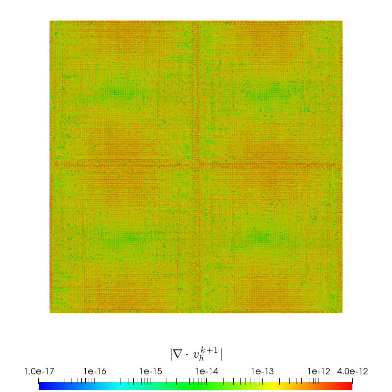
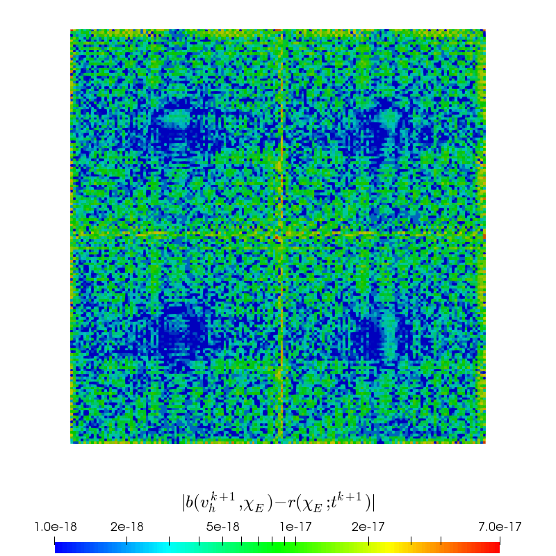
Figure 1: Pointwise divergence (left) and local mass conservation (right) of the 2D Taylor-Green vortex solution at time $t=1$, $\Delta t=0.025$ with the $\mathcal{Q}_{2}/\mathcal{Q}_{1}$ discretization and Helmholtz flux reconstruction in $\text{RT}_{h}^{1}$.
For comparison, the results of the other two discrete Helmholtz decompositions can be found in [28].

4.2 Temporal convergence within the RIPCS

We repeat the numerical convergence tests on the RIPCS that have been carried out in [28], here for the novel Helmholtz flux Raviart-Thomas reconstruction as well. As already indicated by the previous results, the temporal error dominates in the range of those measurements, and hence the errors do not change significantly and convergence rates in time are retained. Thus, we only present an updated analysis with the Beltrami flow in three dimensions using Helmholtz flux reconstruction. For the description of Beltrami flow refer to Section 5.4. Again we set $\rho=\mu=1$ and run computations on $50^{3}$ cubic mesh.

Figure 2 shows the errors and convergence rates as a function of $\Delta t$. The green curves show the $L^{2}$-error for the velocity, the red curves the $H_{0}^{1}$-error for the velocity and the blue curves the $L^{2}$-error for the pressure obtained by the polynomial degrees $p=2,3,4$. Note that for $p=2$ the spatial error in the splitting scheme becomes all-dominant. This emerges at first for the $H_{0}^{1}$-error and $L^{2}$-error on the velocity. For polynomial degree 4, however, the spatial error is negligible and the two error norms on the velocity are perfectly second order convergent in time. The convergence for the pressure in $L^{2}$-norm is close to $\mathcal{O}(\Delta t^{2})$.

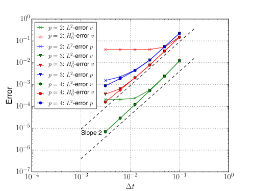
Figure 2: Errors and convergence rates at final time $T=0.5$ for the Beltrami test problem using the spatial discretizations $\mathcal{Q}_{p}/\mathcal{Q}_{p-1}$, $p\in\{2,3,4\}$, and Helmholtz flux reconstruction in $\text{RT}_{h}^{p-1}$.
Previously obtained results with div-div projection can be found in [28].

5 Numerical results

5.1 Implementation

The parallel solver has been implemented in a high-performance C++ code using the object-oriented DUNE finite element framework [44, 45]. The incompressible Navier-Stokes solver described uses the spectral discontinuous Galerkin method on quadrilateral/hexahedral meshes where sum-factorization can be most easily applied to. The complexity reduction in the computation coming from sum-factorization leads to a significant speedup especially for high-order DG methods. Matrix-free methods are thereby put in a superior position to traditional matrix-based methods as matrix entries can be computed faster on-the-fly than loaded from memory. For the representation of function spaces we use tensor product bases built from Gauss-Lobatto-Lagrange polynomials, for the evaluation of integrals we use (non-collocated) Gauss-Legendre quadrature. The pressure Poisson equation, and Helmholtz equation in case of the Stokes equations, are solved with the Conjugate Gradient method and a hybrid AMG-DG preconditioner. This particular DG multigrid algorithm is based on a correction in the conforming piecewise linear subspace where only the low order components are explicitly assembled and the operations on the DG level are done matrix-free. In case of the Navier-Stokes equations, the arising equations in the viscous substep are solved with matrix-free Newton-GMRes. Postprocessing steps like the pressure update that involve a mass matrix only, are solved with the matrix-free inverse mass matrix operator. As preconditioners in the GMRes method or as DG smoothers within the multigrid algorithm, respectively, we employ block Jacobi, Gauss-Seidel or symmetric Gauss-Seidel methods for use in domain decomposition. In order to solve the diagonal blocks, the following approaches have been implemented. In the first (named partially matrix-free), these diagonal blocks are factorized and during preconditioning a forward/backward solve is used. In the second approach the diagonal blocks are solved iteratively using matrix-free sum-factorization. Both of these variants have been developed in [40]. The third variant, however, implements the tensor product preconditioners [46] which are based on Kronecker singular value decomposition (KSVD) of the diagonal blocks.

5.2 Potential flow

We consider the potential flow [12] of the form $v(x,y,t)=t\nabla\chi(x,y)$ with the harmonic potential $\chi(x,y)=5x^{4}y+y^{5}-10x^{2}y^{3}$ such that $\Delta\chi(x,y)=0$. By construction, $v$ is divergence-free and also harmonic. The velocity field solves the instationary Stokes equations on $\Omega=(0,1)^{2}$

$$\partial_{t}v-\nu\Delta v+\nabla p =0$$

$$\nabla\cdot v =0$$

for any viscosity $\nu$ with pressure $p=-\chi$. Global Dirichlet boundary conditions are imposed by the analytical solution. This test case serves as a investigation on pressure robustness for the three variants of Helmholtz decomposition within the RIPCS. It is intended to demonstrate how the velocity errors may depend (or may not depend) on the viscosity. For a pressure robust method, it is expected that these errors are independent on the viscosity.

We simulate the potential flow problem starting from time $t_{0}=0$ up to $T=1$ for different viscosity values $\nu\in\{10^{-1},10^{-2},10^{-3},10^{-4},10^{-5}\}$. We consider the cumulative velocity errors $L^{2}(t_{0},T;L^{2}(\Omega)^{d})$ and $L^{2}(t_{0},T;H_{0}^{1}(\Omega)^{d})$, and the cumulative pressure error $L^{2}(t_{0},T;L^{2}(\Omega))$ for varying spatial resolutions where the time integral is approximated by a trapezoidal rule. Therefore we carry out computations on rectangular meshes with $2^{l+2}$ cells per direction where the level $l$ ranges over $\{1,...,5\}$. To eliminate the temporal error we use a fixed time step size of $\Delta t=5\cdot 10^{-3}$. The upcoming numerical analysis is performed for the polynomial degrees $p=2,3$ as the corresponding velocity ansatz spaces do not represent the exact solution yet.

Table 1 shows the convergence behavior in space for $\nu=10^{-1}$ obtained by the div-div projection. The order of convergence in $L^{2}$ and $H^{1}$ for the velocity, respectively, and for the pressure in $L^{2}$ is optimal as predicted by classical theory. The rates do not deteriorate for smaller viscosity values, though the velocity errors exhibit a growth proportional to the factor $1/\nu$ that comes with the bound including the pressure as can be seen in figure 3. In all the figures presented the green curves show the velocity $L^{2}$-error for 16, 32, 64 cells per direction. The curves in red color show the velocity $H_{0}^{1}$-error, the curves in blue color the pressure $L^{2}$-error for the same spatial resolutions. The numerical results thus indicate that the div-div projection utilized within the RIPCS does not provide a pressure robust splitting scheme. The same conclusion can be drawn from pressure Poisson Raviart-Thomas reconstruction, c.f. with the Table 2 and figure 4. Although not explicitly shown here, we have performed the numerical experiments with the div-div-conti projection. In [47] it was proven for mixed DG discretizations that the viscosity growth of the pressure term in the velocity estimate is reduced to $\nu^{-\frac{1}{2}}$, if both stabilization terms are simultaneously added on quadrilateral/hexahedral meshes. In fact, we observe an increase of the velocity errors close to $\nu^{-\frac{1}{2}}$ for decreasing $\nu$.

level	$L^{2}$-error $v$	$L^{2}$-rate $v$	$H_{0}^{1}$-error $v$	$H_{0}^{1}$-rate $v$	$L^{2}$-error $p$	$L^{2}$-rate $p$
1	1.518e-03		9.307e-02		9.681e-03
2	1.901e-04	2.997	2.343e-02	1.990	2.406e-03	2.009
3	2.371e-05	3.003	5.871e-03	1.996	6.013e-04	2.000
4	2.959e-06	3.002	1.469e-03	1.999	1.503e-04	2.000
5	3.695e-07	3.001	3.675e-04	1.999	3.758e-05	2.000

level	$L^{2}$-error $v$	$L^{2}$-rate $v$	$H_{0}^{1}$-error $v$	$H_{0}^{1}$-rate $v$	$L^{2}$-error $p$	$L^{2}$-rate $p$
1	1.723e-05		1.740e-03		2.927e-04
2	1.089e-06	3.984	2.201e-04	2.983	3.653e-05	3.002
3	6.807e-08	4.000	2.752e-05	3.000	4.544e-06	3.007
4	4.254e-09	4.000	3.439e-06	3.000	5.674e-07	3.001
5	2.661e-10	3.999	4.299e-07	3.000	7.091e-08	3.000

Table 1: Errors accumulated over time and convergence rates for the potential flow problem with $\nu=10^{-1}$ utilizing div-div projection. The top shows results for polynomial degree 2, the bottom for polynomial degree 3.

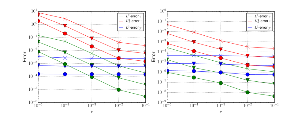
Figure 3: Errors accumulated over time vs. the viscosity parameter $\nu\in\{10^{-5},...,10^{-1}\}$ for the div-div projection on different mesh refinement levels and fixed time step size $\Delta t=5\cdot 10^{-3}$. $(\times)$ denotes the errors for 16 cells per direction (level 2) on the unitsquare,$(\blacktriangledown)$ for 32 cells per direction (level 3) and $(\bullet)$ for 64 cells per direction (level 4).
Left subfigure shows results for $p=2$, right subfigure $p=3$.

level	$L^{2}$-error $v$	$L^{2}$-rate $v$	$H_{0}^{1}$-error $v$	$H_{0}^{1}$-rate $v$	$L^{2}$-error $p$	$L^{2}$-rate $p$
1	9.165e-04		5.165e-02		9.874e-03
2	1.116e-04	3.038	1.256e-02	2.039	2.453e-03	2.009
3	1.368e-05	3.028	3.092e-03	2.023	6.015e-04	2.028
4	1.691e-06	3.016	7.667e-04	2.012	1.503e-04	2.000
5	2.102e-07	3.008	1.909e-04	2.006	3.758e-05	2.000

level	$L^{2}$-error $v$	$L^{2}$-rate $v$	$H_{0}^{1}$-error $v$	$H_{0}^{1}$-rate $v$	$L^{2}$-error $p$	$L^{2}$-rate $p$
1	9.862e-06		8.080e-04		2.902e-04
2	5.635e-07	4.129	9.016e-05	3.164	3.631e-05	2.999
3	3.324e-08	4.083	1.042e-05	3.113	4.539e-06	3.000
4	2.010e-09	4.048	1.242e-06	3.068	5.673e-07	3.000
5	1.237e-10	4.023	1.513e-07	3.037	7.091e-08	3.000

Table 2: Errors accumulated over time and convergence rates for the potential flow problem with $\nu=10^{-1}$ utilizing pressure Poisson Raviart-Thomas projection in $\text{RT}_{h}^{p-2}$. The top shows results for polynomial degree 2, the bottom for polynomial degree 3.

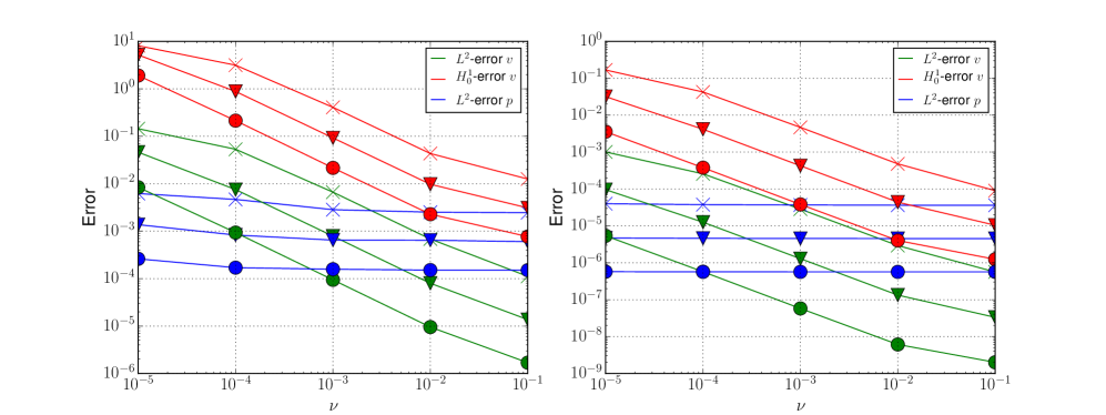
Figure 4: Errors accumulated over time vs. the viscosity parameter $\nu\in\{10^{-5},...,10^{-1}\}$ for the pressure Poisson Raviart-Thomas projection in $\text{RT}_{h}^{p-2}$ on different mesh refinement levels and fixed time step size $\Delta t=5\cdot 10^{-3}$. $(\times)$ denotes the errors for 16 cells per direction (level 2) on the unitsquare,$(\blacktriangledown)$ for 32 cells per direction (level 3) and $(\bullet)$ for 64 cells per direction (level 4).
Left subfigure shows results for $p=2$, right subfigure $p=3$.

level	$L^{2}$-error $v$	$L^{2}$-rate $v$	$H_{0}^{1}$-error $v$	$H_{0}^{1}$-rate $v$	$L^{2}$-error $p$	$L^{2}$-rate $p$
1	1.720e-02		9.861e-01		1.917e-02
2	4.014e-03	2.100	4.929e-01	1.000	2.653e-03	2.853
3	9.950e-04	2.012	2.465e-01	1.000	6.085e-04	2.124
4	2.486e-04	2.001	1.233e-01	1.000	1.508e-04	2.013
5	6.216e-05	2.000	6.163e-02	1.000	3.760e-05	2.004

level	$L^{2}$-error $v$	$L^{2}$-rate $v$	$H_{0}^{1}$-error $v$	$H_{0}^{1}$-rate $v$	$L^{2}$-error $p$	$L^{2}$-rate $p$
1	3.530e-04		3.543e-02		2.958e-04
2	4.357e-05	3.018	9.079e-03	1.964	3.761e-05	2.975
3	5.447e-06	3.000	2.270e-03	2.000	4.686e-06	3.005
4	6.798e-07	3.002	5.652e-04	2.006	5.718e-07	3.035
5	8.496e-08	3.000	1.410e-04	2.002	7.100e-08	3.010

Table 3: Errors accumulated over time and convergence rates for the potential flow problem with $\nu=10^{-1}$ utilizing Helmholtz flux Raviart-Thomas projection in $\text{RT}_{h}^{p-1}$. The top shows results for polynomial degree 2, the bottom for polynomial degree 3.

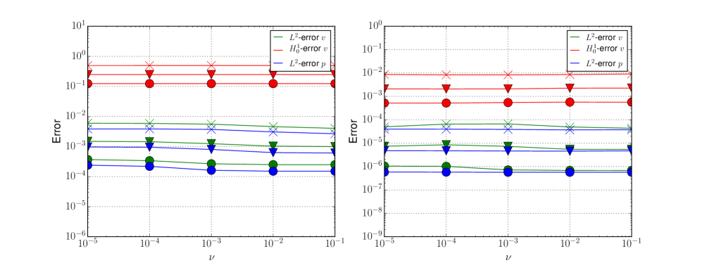
Figure 5: Errors accumulated over time vs. the viscosity parameter $\nu\in\{10^{-5},...,10^{-1}\}$ for the Helmholtz flux Raviart-Thomas projection in $\text{RT}_{h}^{p-1}$ on different mesh refinement levels and fixed time step size $\Delta t=5\cdot 10^{-3}$. $(\times)$ denotes the errors for 16 cells per direction (level 2) on the unitsquare,$(\blacktriangledown)$ for 32 cells per direction (level 3) and $(\bullet)$ for 64 cells per direction (level 4).
Left subfigure shows results $p=2$, right subfigure $p=3$.

Figure 5 shows the dependence of the errors on the viscosity obtained by Helmholtz flux reconstruction, and Table 3 the convergence behavior in space for $\nu=10^{-1}$. Importantly, as can be seen in the figure, the dependence of the velocity errors on the viscosity is visually absent for Helmholtz flux reconstruction. The implementation, however, currently computes a tentative velocity in $X_{h}^{3}$ in order to reconstruct a solenoidal velocity in $\text{RT}_{h}^{2}$, a subject that we will discuss in Section 6. The space $X_{h}^{3}$ delivers one additional approximation order for the velocity compared to $\text{RT}_{h}^{2}$ and therefore we will compare the accuracy to $p=2$ methods. Note that the approximation order for the pressure is unaffected by Helmholtz flux reconstruction. The right subfigure of 5 shows the dependence of errors on $\nu$ for Helmholtz flux reconstruction in $\text{RT}_{h}^{2}$, the left subfigure of 3 the dependence for the spatial discretization with $p=2$ and div-div projection employed. It can be seen that the $H^{1}$- and $L^{2}$-errors for those two methods are of equal magnitude for the largest viscosity value $\nu=10^{-1}$. But eventually for decreasing $\nu$, Helmholtz flux reconstruction in $\text{RT}_{h}^{2}$ outperforms div-div projection with polynomial degree $p=2$ as the $H^{1}$- and $L^{2}$-errors exhibit no growth. The same conclusion can be drawn when comparing to pressure Poisson flux reconstruction.

We have also performed the same tests on a parallelepiped domain $\Omega$. We observe that the velocity errors still remain constant in $\nu$ for domains constructed by affine transformations. The corresponding results have been left out since they do not differ significantly compared to those in figure 5. The numerical experiments thereby indicate that Helmholtz flux Raviart-Thomas projection utilized within the RIPCS provides a pressure robust splitting scheme.

Potential flow with irrotational force translation

To see how a discretization scheme fulfills the invariance property, consider the potential flow problem with a irrotational source term $f=\nabla\psi$. As proposed in [48], we choose $\psi(x,y)=\exp(-10(1-x+2y))$. With this source term the instationary Stokes equations

$$\partial_{t}v-\nu\Delta v+\nabla p =f$$

$$\nabla\cdot v =0\;.$$

have the exact solution $v=t\nabla\chi$ and $p=-\chi+\psi$. We have repeated the numerical experiments to verify if the splitting schemes offer a invariance property or how far they deviate from it depending on the viscosity. The numerical results demonstrate that the div-div and pressure Poisson Raviart-Thomas projection do not yield a pressure robust splitting scheme because the velocity errors are constantly higher as for the zero right-hand side. Moreover, the velocity errors show the same growth in inverse proportion to the viscosity. In contrast, the velocity errors for the Helmholtz flux Raviart-Thomas projection appear to be robust in pressure and viscosity.

5.3 Gresho vortex

The Gresho vortex has been recently proposed as model problem in [8] for investigating how well a discretization scheme preserves structures. It is argued that a pressure robust method in this regard is in general superior to a non pressure robust method such that the latter has certain difficulties preserving the vortex structure of this flow. Centered at $c=(0.5,0.5)^{T}$ with constant translational velocity $w_{0}\in\mathbb{R}^{2}$ (called wind), the setup is described by the initial condition

$$v_{0}(x)=w_{0}+\begin{cases}(-5\tilde{x}_{2},5\tilde{x}_{1})^{T}&,0\leq r<0.2\\ \left(-\frac{2\tilde{x}_{2}}{r}+5\tilde{x}_{2},\frac{2\tilde{x}_{1}}{r}-5\tilde{x}_{1}\right)^{T}&,0.2\leq r<0.4\\ 0&,0.4\leq r\end{cases}$$ (23)

with shifted coordinates $\tilde{x}=x-c$ towards the center, $r=\left\|\tilde{x}\right\|_{2}$. The initial Gresho vortex satisfies $\nabla\cdot v_{0}=0$. In the core $r<0.2$ the vorticity $\nabla\times v_{0}$ is constantly 10.0, decreases linearly in the circular ring $0.2\leq r<0.4$, and vanishes for $r\geq 0.4$. The initial vorticity is displayed in figure 6 where the discontinuities at the two aforementioned shells are visible.

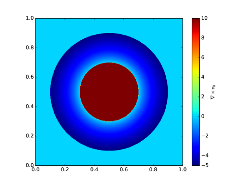
Figure 6: Vorticity of the initial Gresho vortex state.

The initial state is evolved in time by the Navier-Stokes equations

$$\partial_{t}v-\nu\Delta v+(v\cdot\nabla)v+\nabla p =0$$

$$\nabla\cdot v =0$$

in the periodic square $\Omega=(0,1)^{2}$. As in [8] we set the viscosity to $\nu=10^{-5}$. For the standing Gresho vortex with $w_{0}=0$ the convection term $(v_{0}\cdot\nabla)v_{0}$ can be balanced by the gradient of a pressure $p_{0}$, $(v_{0}\cdot\nabla)v_{0}=-\nabla p_{0}$, and, consequently, the standing Gresho vortex describes a steady solution to the instationary Euler equations. With the diffusion term $-\nu\Delta v$ added, the Navier-Stokes problem smoothes out the discontinuities from the initial condition. Now, the choice $w_{0}=(1/3,1/3)^{T}$ is referred to as the moving Gresho vortex that we will consider in this work. In this case the vorticity distribution is transported in the top-right direction through the periodic domain such that the vortex at time $T=3$ is intended to be again centered around $c=(0.5,0.5)^{T}$.

We simulate the moving Gresho vortex problem from time $t_{0}=0$ up to $T=3$ utilizing the three variants of discrete Helmholtz decomposition within the RIPCS for the polynomial degrees 4 and 8. For $p=4$ we use a spatial resolution of 32 cells per direction, for $p=8$ 16 cells per direction. All runs have been performed with a fixed time step size of $\Delta t=2\cdot 10^{-3}$.

Let us start the discussion on the numerical results by considering important flow quantities for each of the simulation performed. In figure 7 the kinetic energy $E(t)=\frac{1}{2}(v_{h},v_{h})_{0,\Omega}$ and enstrophy $\mathcal{E}(t)=\frac{1}{2}(\nabla_{h}\times v_{h},\nabla_{h}\times v_{h})_{0,\Omega}$ are displayed over time.

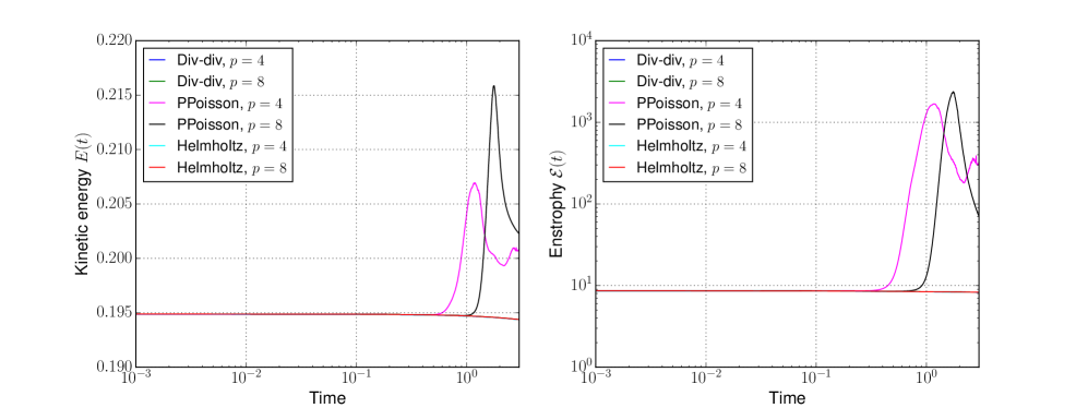
Figure 7: Evolution of kinetic energy (left) and enstrophy (right) for the $\mathcal{Q}_{p}/\mathcal{Q}_{p-1}$ pairs $(p\in\{4,8\})$ and respective discrete Helmholtz decompositions. Helmholtz in the legend abbreviates the reconstruction of the Helmholtz flux in $\text{RT}_{h}^{p-1}$, and PPoisson the reconstruction of the pressure Poisson flux in $\text{RT}_{h}^{p-2}$. Note that the evolution obtained by div-div projection and Helmholtz flux reconstruction are almost indistinguishable.

At the beginning all kinetic energy curves remain very close to constant as expected for this low viscosity value. However, towards the end, the computations performed with the pressure Poisson Raviart-Thomas reconstruction show an increase which is nonphysical for this freely evolving system. The same observation can be made for the enstrophy which in theory cannot increase as well in two dimensions. The div-div projection and Helmholtz flux Raviart-Thomas reconstruction deliver stable results which are close to the Scott-Vogelius computations in [8]. This comparison shows that in terms of conserved quantities for inviscid flows, the splitting scheme realized by pressure Poisson Raviart-Thomas projection is outperformed by the other two variants.

Now, let us investigate the vorticity plots at time $T=3$ for the three discrete Helmholtz decompositions. Figure 8- 10 show the results for the polynomial degree 4 (left subfigures) and $p=8$ (right subfigures). One

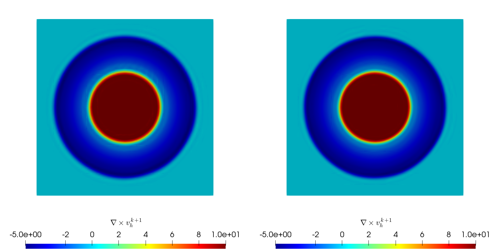
Figure 8: Vorticity of moving Gresho vortex at time $T=3$ by $\mathcal{Q}_{p}/\mathcal{Q}_{p-1}$ discretization with div-div projection. Left part shows $p=4$ method (32 cells per direction), right part the $p=8$ method (16 cells per direction).

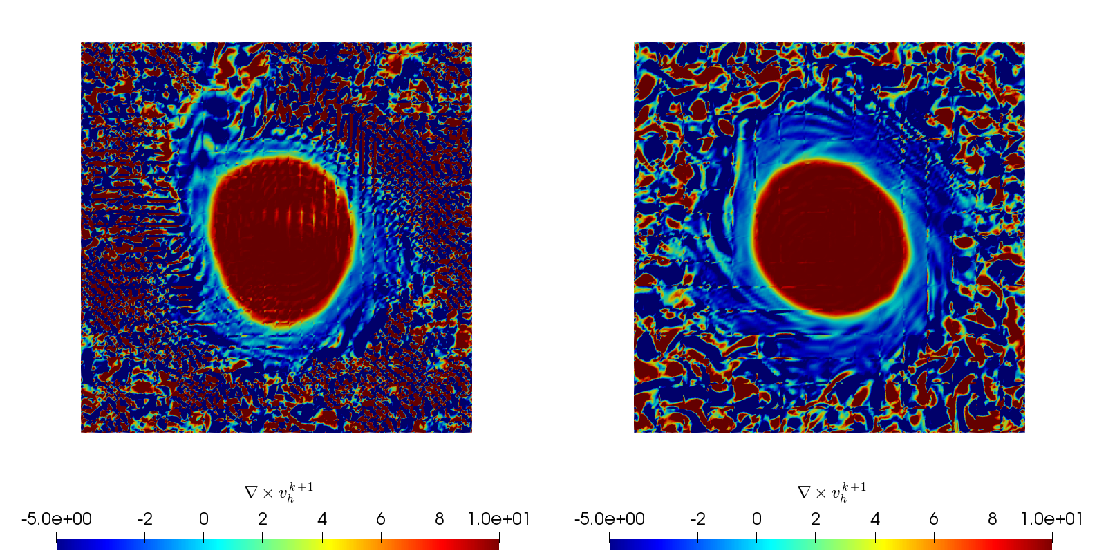
Figure 9: Vorticity of moving Gresho vortex at time $T=3$ by $\mathcal{Q}_{p}/\mathcal{Q}_{p-1}$ discretization with pressure Poisson Raviart-Thomas reconstruction in $\text{RT}_{h}^{p-2}$. Left part shows $p=4$ method (32 cells per direction), right part the $p=8$ method (16 cells per direction).

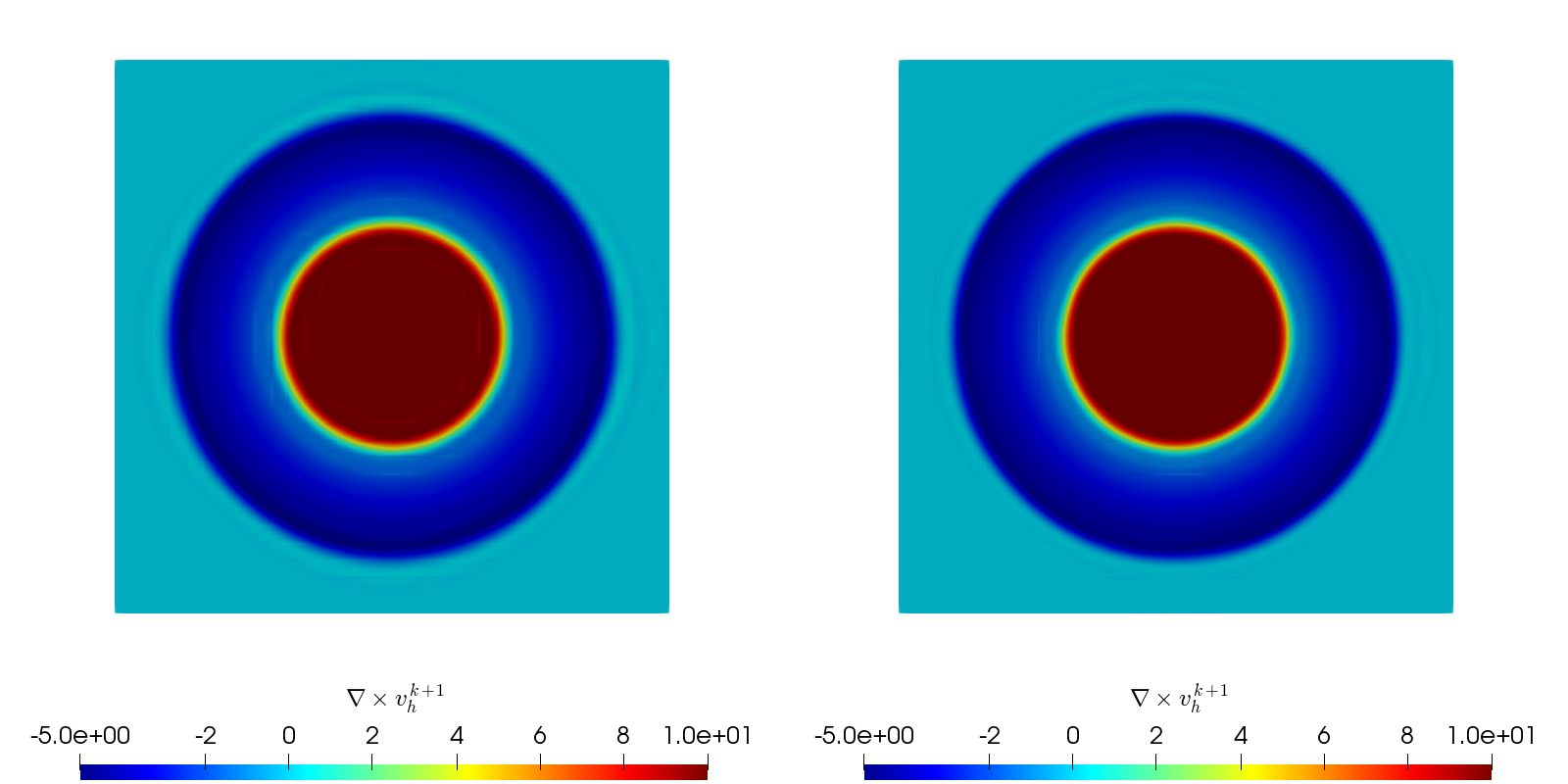
Figure 10: Vorticity of moving Gresho vortex at time $T=3$ by $\mathcal{Q}_{p}/\mathcal{Q}_{p-1}$ discretization with Helmholtz flux Raviart-Thomas projection in $\text{RT}_{h}^{p-1}$. Left part shows $p=4$ method (32 cells per direction), right part the $p=8$ method (16 cells per direction).

can observe that div-div projection and Helmholtz flux Raviart-Thomas projection are able to preserve the structure of the initial condition whereas the simulations with pressure Poisson reconstruction are interspersed with instabilities away from the vortex core. These numerical artifacts are eventually responsible for the nonphysical growth in kinetic energy and enstrophy. Furthermore, one can see that the higher order method with $p=8$ gives for both stable variants slightly better results in terms of over-/under-shoots. On the one hand, this is surprising as the initial condition is discontinuous and the flow is governed by inviscid vortex transport, but on the other hand viscous diffusion - no matter how small - eventually provides sufficient regularity of the problem. As above we can conclude that the non pressure robust splitting scheme with pressure Poisson reconstruction is inferior in preserving structures with large gradient parts. We also want to point out that the effect of div-div stabilization gives similar results to those obtained by a pressure robust method, c.f. figures 8 and 10. This observation has been made with respect to grad-div stabilization in the literature.

5.4 Beltrami flow

The Beltrami flow is one of the rare test problems that describes a fully three-dimensional solution of the instationary Navier-Stokes equations. It has been derived as a class of analytical solutions in [49] by separation of variables. The velocity field and pressure read

$$\begin{split}v_{1}(x,y,z,t)&=-a\,e^{-\nu d^{2}\,t}\,\left(e^{a\,x}\,\sin\left(d\,z+a\,y\right)+\cos\left(d\,y+a\,x\right)\,e^{a\,z}\right)\\ v_{2}(x,y,z,t)&=-a\,e^{-\nu d^{2}\,t}\,\left(e^{a\,x}\,\cos\left(d\,z+a\,y\right)+e^{a\,y}\,\sin\left(a\,z+d\,x\right)\right)\\ v_{3}(x,y,z,t)&=-a\,e^{-\nu d^{2}\,t}\,\left(e^{a\,y}\,\cos\left(a\,z+d\,x\right)+\sin\left(d\,y+a\,x\right)\,e^{a\,z}\right)\\ p(x,y,z,t)&=p_{0}(t)-0.5\,a^{2}\,\rho\,e^{-2\nu d^{2}\,t}\,(2\,\cos\left(d\,y+a\,x\right)\,e^{a\,\left(z+x\right)}\,\sin\left(d\,z+a\,y\right)\\ &\quad+2\,e^{a\,\left(y+x\right)}\,\sin\left(a\,z+d\,x\right)\,\cos\left(d\,z+a\,y\right)\\ &\quad+2\,\sin\left(d\,y+a\,x\right)\,e^{a\,\left(z+y\right)}\,\cos\left(a\,z+d\,x\right)+e^{2\,a\,z}+e^{2\,a\,y}+e^{2\,a\,x})\end{split}$$ (24)

where $p_{0}(t)$ is chosen to ensure $\int_{\Omega}p(x,y,z,t)\mathrm{d}x\mathrm{d}y\mathrm{d}z=0$ over time. The Beltrami flow solves the instationary Navier-Stokes equations for any positive viscosity $\nu>0$. The computational domain is given by $\Omega=(-1,1)^{3}$. On $\partial\Omega$ Dirichlet boundary conditions for the velocity are imposed by the exact solution. The Beltrami flow has the property that the velocity and vorticity vectors are aligned, i.e. $d\;v-\nabla\times v=0$, and that the nonlinear convection term is balanced by the pressure gradient, $\rho(v\cdot\nabla)v=-\nabla p$. It is therefore interesting to see how a discretization handles the irrotational part for $\nu\ll 1$.

Inspired by the tests in [9, 8] we set the parameters $a=\pi/4,\;d=\pi/2$ and simulate the Beltrami problem for $\nu\in\{1,10^{-3}\}$ from time $t_{0}=0$ up to $T=1$. We set the polynomial degree for the velocity DG space to $p=4$ and use a mesh resolution of 8 cells per direction. To eliminate instabilities from the time-stepping we set $\Delta t=10^{-3}$. Figure 11 shows the $|(v-v_{h})(t)|_{1,\Omega}$ errors over time for the three variants of discrete Helmholtz decomposition. The progression of the $L^{2}$-norm only differs in absolute values and has been omitted.

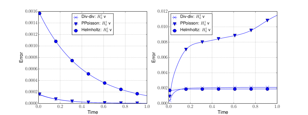
Figure 11: Plots of time versus $H_{0}^{1}(\Omega)$-velocity error for the three variants of discrete Helmholtz decomposition. Left part shows progression for $\nu=1$, right part for $\nu=10^{-3}$

One can observe that with $\nu=1$ all splitting methods remain accurate (at the level of spatial approximation error) up to the end time. The right subfigure shows the corresponding results for viscosity $10^{-3}$ where no such rapid exponential decay of the errors is expected. Note that the initial errors are the same for all runs but the y-scale has been enlarged accordingly. However, we observe that the $H^{1}$-seminorm errors for pressure Poisson Raviart-Thomas projection grow in time and the solution becomes inaccurate. As stated in the previous section, div-div projection improves the results such that only at the beginning an increase is visible. In contrast, Helmholtz flux Raviart-Thomas projection within the RIPCS provides constant $|(v-v_{h})(t)|_{1,\Omega}$ errors and, apart from the first time steps, outperforms the div-div projection in this measure. We conclude that Helmholtz flux reconstruction which is indicated to give a pressure robust splitting scheme reproduces well this (seemingly) easy flow problem.

5.5 3D Taylor-Green vortex

The three-dimensional Taylor-Green vortex is aimed at testing the accuracy and performance of high-order methods in a DNS. The flow starts from a simple large scale initial condition. In the early phase it undergoes vortex stretching until laminar breakdown before the maximum dissipation of the fluid is reached. The flow then transitions to turbulence followed by a decay phase of eventually Homogeneous Isotropic Turbulence (HIT). The problem originates from [50] where classes of sinusoidal fields were considered as an initial condition that satisfy the continuity equation $\nabla\cdot v=0$. It has been proposed as a reference benchmark since the first edition of the international workshop on High-Order CFD Methods and is quoted in [51], C3.5, for instance.

The simulation domain is $\Omega=(-\pi L,\pi L)^{3}$ with periodic boundary conditions in all directions and no external forcing, $f=0$. The initial flow field is given by

$$\begin{split}v_{0}(x)\cdot e_{1}&=V_{0}\sin\left(\frac{x_{1}}{L}\right)\cos\left(\frac{x_{2}}{L}\right)\cos\left(\frac{x_{3}}{L}\right)\\ v_{0}(x)\cdot e_{2}&=-V_{0}\cos\left(\frac{x_{1}}{L}\right)\sin\left(\frac{x_{2}}{L}\right)\cos\left(\frac{x_{3}}{L}\right)\\ v_{0}(x)\cdot e_{3}&=0\end{split}$$ (25)

$$p_{0}(x) =p_{0}+\frac{\rho_{0}V_{0}^{2}}{16}\left(\cos\left(\frac{2x_{1}}{L}\right)+\cos\left(\frac{2x_{2}}{L}\right)\right)\left(\cos\left(\frac{2x_{3}}{L}\right)+2\right)\;.$$ (26)

The Reynolds number of the flow here is defined as $\text{Re}=\frac{\rho_{0}V_{0}L}{\mu}$. As in the references [51, 52] we set $L=1,\;V_{0}=1,\;\rho_{0}=\rho=1,\;p_{0}=0,\;\textup{Re}=1600$.

Using this problem we want to demonstrate that with a pressure robust DG method, a robust method for underresolved turbulent incompressible flows can be realized. To this end, we have done computations on a series of uniformly refined, equidistant cuboid meshes for different polynomial degrees. There are detailed reference data available which contain the temporal evolution of

• kinetic energy $E(t)=\frac{1}{\rho_{0}\left|\Omega\right|}\frac{1}{2}(\rho v_{h},v_{h})_{0,\Omega}$,

• dissipation rate $\epsilon(t)=\frac{\nu}{\left|\Omega\right|}(\nabla_{h}v_{h},\nabla_{h}v_{h})_{0,\Omega}$,

• enstrophy $\mathcal{E}(t)=\frac{1}{\rho_{0}\left|\Omega\right|}\frac{1}{2}(\rho\nabla_{h}\times v_{h},\nabla_{h}\times v_{h})_{0,\Omega}$

in the time interval $[0,20t_{c}]$ where $t_{c}=\frac{L}{V_{0}}$ is the convective time unit. The reference values were obtained with a dealiased pseudo-spectral code run on $512^{3}$ grid, time integration was performed with a low-storage three-step Runge-Kutta method and a time step $\Delta t=10^{-3}\,t_{c}$. We will concentrate on the results of kinetic energy dissipation $\epsilon(t)$, and the spectral distribution of kinetic energy $E(k,t)$ s.t. $E(t)=\int_{0}^{\infty}E(k,t)\mathrm{d}k$ at $t=9t_{c}$, close to the maximum amount of dissipation. Table 4 summarizes configurations, including variant of discrete Helmholtz decomposition, number of cells per direction, polynomial degree and velocity DOFs.

Helmholtz flux reconstruction	Cells per direction	$p$	Velocity DOFs
	8	7	64
	16	3	64
	16	7	128
	32	3	128
	48	4	240
	64	3	256
	128	3	512
Pressure Poisson reconstruction	Cells per direction	$p$	Velocity DOFs
	16	3	64
	32	3	128
	40	3	160
	64	3	256
	128	3	512

Table 4: Grid configurations for 3D Taylor-Green problem.

We compare the results with the reference solution in figure 12. The top left shows dissipation curves for different grid sizes and polynomial degree 3, including a fully resolved simulation with $p=4$ and 240 velocity DOFs. The dashed lines here refer to pressure Poisson Raviart-Thomas projection. It can be seen that the corresponding underresolved simulations (dashed lines, black color) are unstable which is caused by a crash of the computation during build-up phase. The runs with 40 and 64 cells per direction (dashed lines in orange and magenta color) describe essentially resolved simulations and already capture the shape from the reference solution. The progression of the curves are similar to the ones obtained in [25] by a standard DG discretization with no additional stabilization terms (c.f. figure 6 in this publication). In contrast, Helmholtz flux Raviart-Thomas projection provides successful underresolved simulations for the two configurations: $p=3$, 16 and 32 cells per direction. The solid lines show the progression using this variant and one can observe that kinetic energy dissipation is stronger underpredicted, the lower the spatial resolution is (c.f. with figure 6 in [25]). The lop left plot shows a zoom around the maximum amount of dissipation where the underresolved runs have been left out.

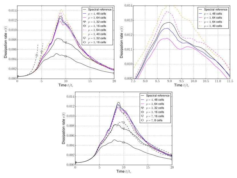
Figure 12: Time evolution of kinetic energy dissipation for the 3D Taylor-Green vortex. Comparison of various DG configurations with reference solution: In the upper plots the dashed lines refer to pressure Poisson Raviart-Thomas projection, and the solid lines using Helmholtz flux reconstruction. In the bottom center plot the solid lines correspond to the same configuration as above, but the dashed lines now correspond to a $p=7$ run with Helmholtz flux reconstruction employed as well.

The bottom center plot shows simulations with the Helmholtz flux reconstruction only employed. Here, the dashed lines show the results of the order $p=7$ method with the same number of velocity DOFs as for the $p=3$ underresolved computations. One can see that the $p=7$ method with 64 velocity DOFs gives results with the same accuracy as the $p=3$ with 128 velocity DOFs. Moreover, the $p=7$ method with 128 velocity DOFs closely matches the simulations with $p=4$, 240 velocity DOFs, which itself is more accurate than the simulation with $p=3$, 256 velocity DOFs. Hence, we also observe the improved accuracy per degree of freedom for higher polynomial $p$ which motivates the use of high-order methods for smooth problems. We further point out that the behavior of our dissipation curves for different $p$ and grid size $h$ matches the enstrophy curves presented in [46].

The kinetic energy spectra computed at $t=9t_{c}$ for the above presented grid configurations are displayed in the figures 13- 15. An approximation quality of a CFD method is to at first reproduce the schematic distribution of spectral energy caused by the three regimes in a turbulent flow. In explicit, a curve shall exhibit an integral range at smallest wavenumbers, a power law in wavenumbers representing the inertial range and a rapid decay at smallest wavenumbers used for the computation.

Figure 13 shows the spectral distribution at time $t=9t_{c}$ for polynomial degree $p=3$ under $h$-coarsening. A DNS simulation with 512 velocity

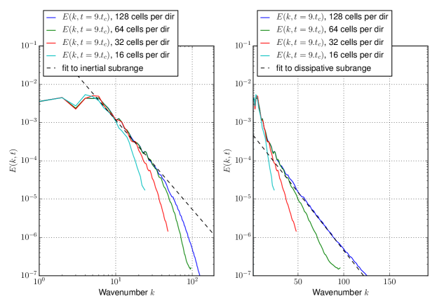
Figure 13: Kinetic energy spectra of the 3D Taylor-Green vortex at $t=9t_{c}$ for polynomial degree $p=3$ under $h$-coarsening, with fits to the inertial and dissipative subrange. All DG configurations here use Helmholtz flux reconstruction in $\text{RT}_{h}^{p-1}$.

DOFs has been added including fits to the inertial and dissipative subrange, respectively. The distribution of $E(k,t)$ should ideally be a decaying power law in the numerically resolved inertial subrange, smaller scales below the effective resolution should be suppressed as if they belong to the dissipative subrange. This is indeed the case as largest scales that are resolved by all configurations, give the same progression at smallest wavenumbers. There are no oscillations for the underresolved computations in the shorter inertial range. Moreover, the higher modes below each discretization resolution are suppressed by an exponential drop which can be seen in a log-lin plot of the same range on the right half. The lower the accuracy is, preferably the more corresponding wavenumbers get dissipated in the grid convergence results.

Figure 14 shows $E(k,t=9t_{c})$ under simultaneous $p$-refinement and $h$-coarsening. As in the previous plot, the green curve represents the

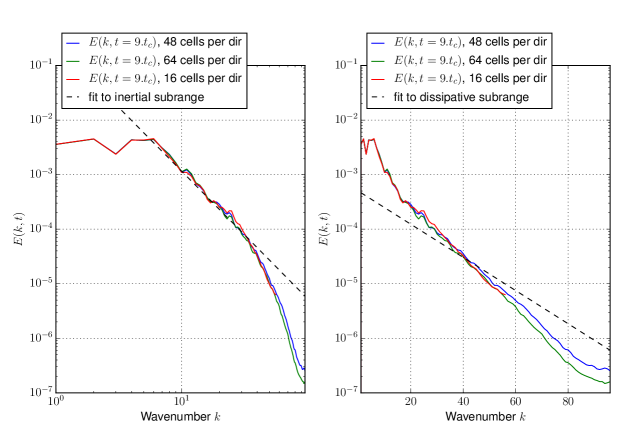
Figure 14: Kinetic energy spectra at $t=9t_{c}$ under simultaneous $p$-refinement and $h$-coarsening. Green curve: $p=3$ and 256 velocity DOFs. Blue curve: $p=4$ and 240 velocity DOFs. Red curve: $p=7$ and 128 velocity DOFs. All DG configurations here use Helmholtz flux reconstruction in $\text{RT}_{h}^{p-1}$.

spectrum with effective resolution of 256 velocity DOFs for $p=3$. We observe that the spectra are almost identical. The $p=7$ method with about half velocity DOFs closely matches the spectral distribution of the other shown configurations up to the beginning of the dissipative subrange. Since the $p=7$ configuration has approximately half as many velocity DOFs, observe that fewer wavenumbers are considered for the Fourier transform.

In figure 15 the distribution of spectral energy for configurations with same amount of velocity DOFs is displayed. For comparison, the fully resolved

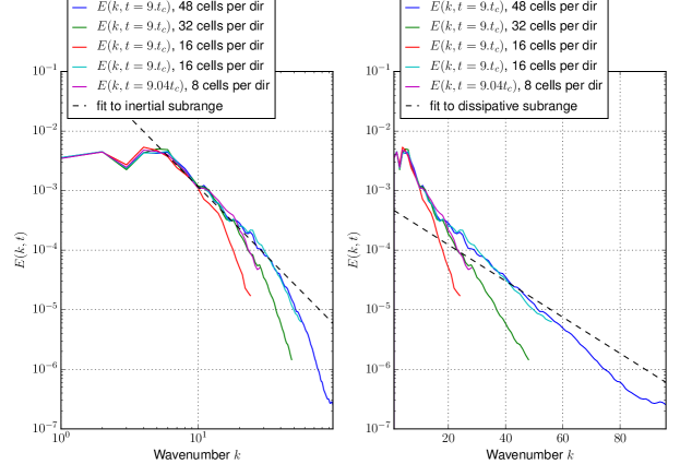
Figure 15: Kinetic spectra at $t=9t_{c}$ computed for varying $p$ and $h$, but same number of velocity DOFs. The fully resolved simulation with $p=4$ has been added for comparison. All DG configurations here use Helmholtz flux reconstruction in $\text{RT}_{h}^{p-1}$.

simulation with $p=4$ has been added as in the previous plot (both curves in blue color). Similar to the $h$-coarsening study, the underresolved computations preferably have the same kinetic energy spectrum up to the corresponding numerical dissipation wavenumber, followed by a rapid decay afterwards. As already observed for the dissipation rate, the result for $p=7$ with 64 velocity DOFs closely matches the result for $p=3$ with twice the velocity DOFs. The configuration $p=7$ with 128 velocity DOFs furthermore reproduces the spectral energy of a resolved simulation ($p=4$, 240 velocity DOFs)

Based on the overall results, we conclude that the DG splitting scheme with Helmholtz flux Raviart-Thomas projection - which evidences to be pressure robust - can be used as a turbulence model in a large-eddy simulation with no additional modification.

6 Conclusion and outlook

We described a novel postprocessing technique in the projection step of splitting schemes for incompressible flow that reconstructs the Helmholtz flux in $H(\text{div})$ and is computed locally. The resulting velocity field satisfies the discrete continuity equation, and is pointwise divergence-free. We performed several numerical experiments with the pressure correction scheme realized by this discrete Helmholtz decomposition, and compared to other discrete Helmholtz decompositions with respect to accuracy in space. The other variants include a previously introduced $H(\text{div})$ postprocessing based on reconstructing the solution to the pressure Poisson equation, and stabilization-enhanced projections. The $H(\text{div})$ postprocessing technique presented in this paper shows to give a high-order DG, pressure robust in space, splitting scheme. Employing sole reconstruction of the pressure Poisson flux in contrast has been found to provide a non pressure robust splitting scheme. The results of the numerical tests illustrate that pressure robust methods outperform non pressure robust methods, especially at high Reynolds numbers. The main reason is that in the incompressible Euler limit for $f=0$, the material derivative is a gradient field which can be handled more appropriately by pressure robust methods. We have also observed that penalized as div-div projection do not cure a lack of pressure robustness, but can counteract so in order to give similar results to those obtained by a pressure robust method. With the 3D Taylor-Green vortex we have included a commonly used benchmark for underresolved turbulence computations. We compared the stability of the two considered reconstruction approaches for various resolutions. The results demonstrate that explicit turbulence modeling in a DG method is not needed, but pressure robustness is a essential ingredient to realize a robust method for underresolved turbulent incompressible flows.

Apart from the growth of the velocity errors for $\nu\rightarrow 0$, the numerical results in this article obtained by div-div projection are equally comparable to Helmholtz flux reconstruction. For the Helmholtz flux reconstruction in the Raviart-Thomas space of degree $p-1$, the implementation currently computes a tentative velocity which is in the DG space of polynomial degree $p$. A possible direction for future work is thus to discretize the viscous substep with the anisotropic tensor product polynomials spanning the local Raviart-Thomas space of degree $p-1$. However, the change to anisotropic tensor product polynomials in our spectral DG implementation would produce a significant amount of additional low-level optimizations leading to sophisticated code which is hard to maintain. Simultaneous work on a Python-based code generator that can transform a very abstract description of the variational form into highly optimized code has been shown to give promising results, [53].

References

-
[1]
G. Katul, A. Porporato, D. Cava, M. Siqueira,
An
analysis of intermittency, scaling, and surface renewal in atmospheric
surface layer turbulence, Physica D: Nonlinear Phenomena 215 (2) (2006) 117
– 126.
doi:https://doi.org/10.1016/j.physd.2006.02.004.
URL http://www.sciencedirect.com/science/article/pii/S0167278906000613 - [2] S.-M. Piatkowski, A Spectral Discontinuous Galerkin method for incompressible flow with Applications to turbulence, Ph.D. thesis, Heidelberg University (2019). doi:https://doi.org/10.11588/heidok.00026674.
-
[3]
A. H. Al-Yaarubi, C. C. Pain, C. A. Grattoni, R. W. Zimmerman,