Seek and You Will Find: A New Optimized Framework for Efficient Detection of Pedestrian

Abstract.

Studies of object detection and localization, particularly pedestrian detection have received considerable attention in recent times due to its several prospective applications such as surveillance, driving assistance, autonomous cars, etc. Also, a significant trend of latest research studies in related problem areas is the use of sophisticated Deep Learning based approaches to improve the benchmark performance on various standard datasets. A trade-off between the speed (number of video frames processed per second) and detection accuracy has often been reported in the existing literature. In this article, we present a new but simple deep learning based strategy for pedestrian detection that improves this trade-off. Since training of similar models using publicly available sample datasets failed to improve the detection performance to some significant extent, particularly for the instances of pedestrians of smaller sizes, we have developed a new sample dataset consisting of more than 80K annotated pedestrian figures in videos recorded under varying traffic conditions. Performance of the proposed model on the test samples of the new dataset and two other existing datasets, namely Caltech Pedestrian Dataset (CPD) and CityPerson Dataset (CD) have been obtained. Our proposed system shows nearly 16% improvement over the existing state-of-the-art result.

1. Introduction

In the area of computer vision and related research, pedestrian detection is an important object localization problem due to its notable application potentials. Acceptably accurate detection of pedestrians in video frames of road scenes still remains a challenging problem due to the enormous variations in the instances of pedestrians with respect to their size, pose, lighting condition, proportion of the occluded parts etc. Study of recent literature shows that deep learning based models are capable of producing improved results over the traditional methods. However, there are a few important concerns related to deep learning based strategies. One of them is the complexity of the model in terms of the number of its trainable parameters and consequently requirement of the computational resources. Often such a model requires multiple processing units, considerably large amount of memory and an efficient parallel computation framework for its simulation. Also, a large amount of labelled data is crucial for effective training of the network. Another issue is the trade-off between computational speed measured by FPS (frames processed per second) and the accuracy of estimation of bounding box around the pedestrian figures which is expressed as Miss Rate (MR). It is clear that simultaneous improvement of both FPS and MR is a challenging task. Contribution of the present study is threefold. Firstly, it describes a new deep architecture (detailed in Sec. 4) requiring less computational resources compared to the existing state-of-the-art models. Secondly, our model is capable of optimizing the trade-off between FPS and MR providing significant improvement in accuracy over existing heavy weight models. This has been described in details in Sec. 5. Finally, we have developed a new sample dataset consisting of little more than 80K annotated pedestrian figures. The images in this dataset are high resolution video frames captured under various traffic conditions. Further details of this new dataset are provided in Sec. 3.

A state of the art Pedestrian Detection system should have the following qualities:

• Precision of recognition in each frame of a video must be guaranteed. This is measured by the well known metric Miss Rate. In real life scenarios precision of recognition is affected due to unknown number of pedestrians, different size of pedestrian images due to physical dimension and their varying distances from the focus of the camera. Also, recognition accuracy plummets due to poor lighting condition and proportion of occluded part (Fig. 1).

  

  

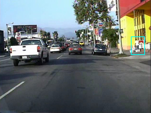
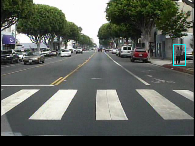
  Variation in lighting condition

  

  

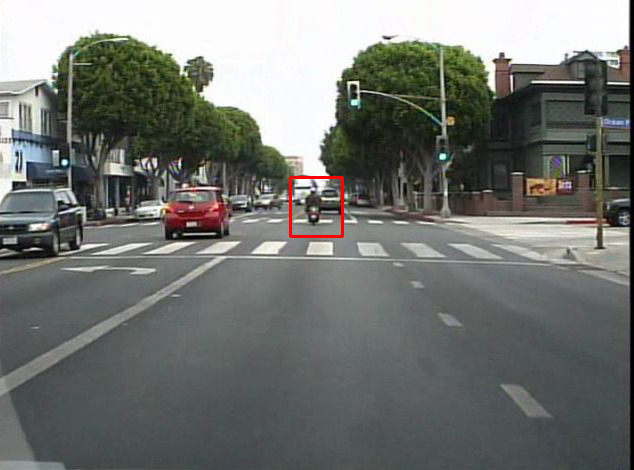
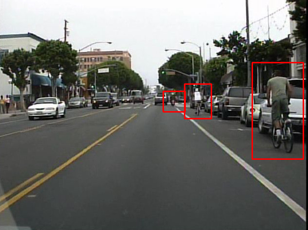
  Variation in pedestrian size

  

  

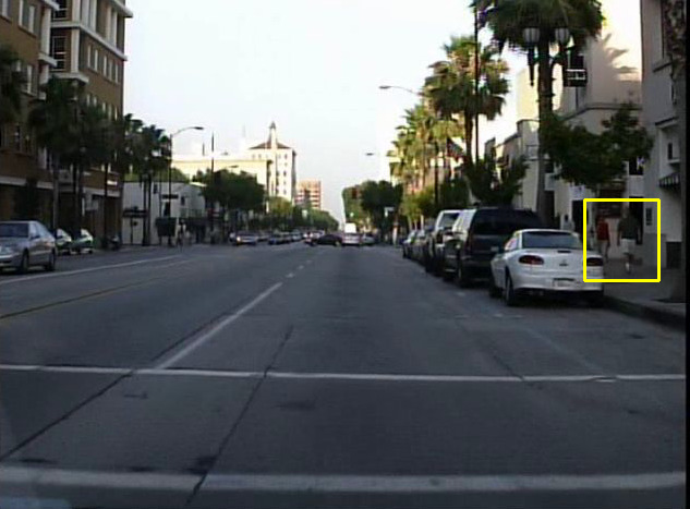
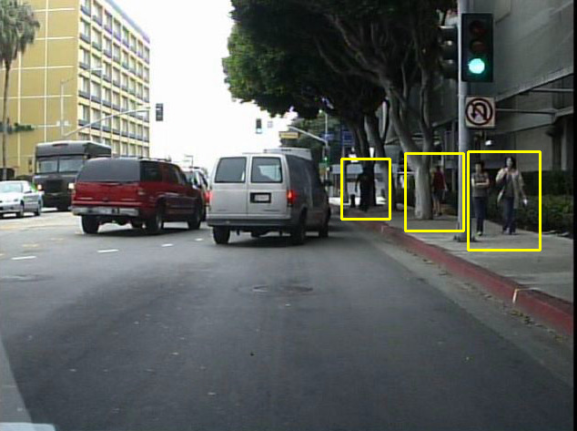
  Variation in occlusion by human body

  

  

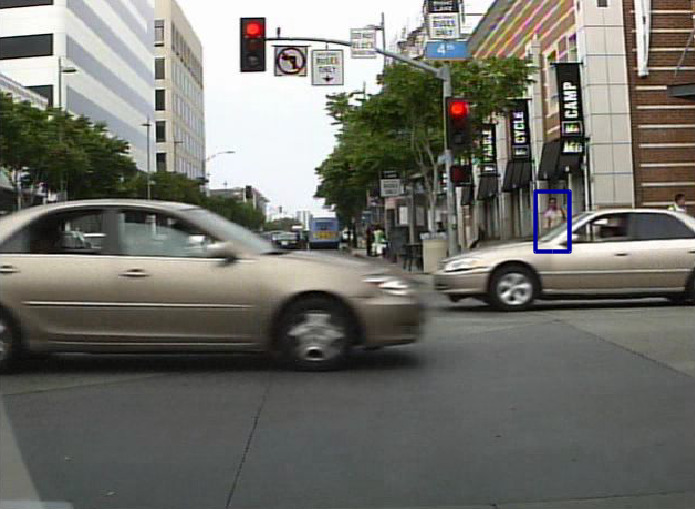
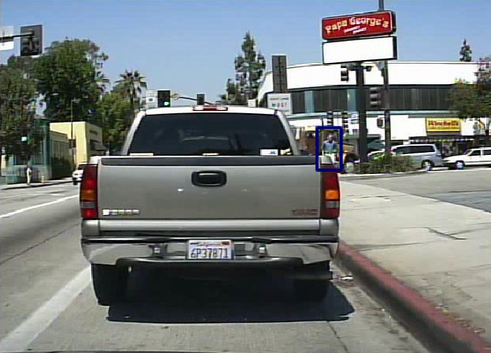
  Variation of occlusion by non-human body

  Figure 1. A few examples of the challenges of existing Caltech Pedestrian Dataset

  Also detecting pedestrians in a dynamic background (camera set in a moving car) is more difficult than detecting the same in a static background (fixed traffic camera). It is noteworthy that the resolution of the camera is also an important factor to accurately detect a pedestrian. Many traditional and deep learning based approaches are exploited to find a generic solution of this problem.

• Real time detection of pedestrian is an even more challenging task. But this is required if we need to incorporate the detection algorithm in a real life system. This is usually measured by Frames per Second (FPS). It is very challenging to implement a network that produce results with a very low MR (high recognition accuracy, for an ideal system this should be 0) and at the same time very high FPS. It is obvious that higher recognition accuracy needs more processing time per frame which on the other hand decreases FPS. This trade-off can be managed to some extent by providing large computational resources which is not available in general purpose systems.

In the present work we have taken care of both these issues and compared the performance of our model with respect to FPS and MR to other benchmark results.

2. Related Works

The relevant studies in this field aim for optimizing miss-rate and real time processing performance. A number of strategies of pedestrian detection have been proposed in the literature. But it is hard to improve both miss-rate and processing speed simultaneously. SVM (Support Vector Machine) trained on HOG (histogram oriented gradients) features is a popularly chosen classifier and some significant studies under this framework had been reported in (Dollar et al., 2012), (Alonso et al., 2007) and (Xu et al., 2005). Some other similar studies were reported in (Tuzel et al., 2008) and (Dalal and Triggs, 2005) as well. Benenson et al. (Benenson et al., 2012) proposed a method without using any deep learning architecture for real time processing which could process 135 frames per second but the miss-rate was noted to be as high as 42%. Ding et al. and Xiao et al. had used certain Contextual Boost method (Ding and Xiao, 2012) with the help of an AdaBoost Classifier (Freund, 2001) to improve the performance of pedestrian detection based on contextual information and achieved a miss-rate of 25%. Convolutional neural network (CNN) based classifiers have already established their efficiency in pedestrian detection tasks (Luo et al., 2014) (Ren et al., 2015) (Angelova et al., 2015). Vanilla Faster R-CNN had performance limitation on Caltech pedestrian dataset due to smaller sizes of pedestrians. Later, He et al. improved this Faster R-CNN strategy with the help of the (RPN + BF(Appel et al., 2013)) (Zhang et al., 2016) to reduce the miss rate but it could process only 2 frames per second with a miss-rate of 9.6% which is the present state-of-the-art of pedestrian detection. Several deep learning based models have been proposed to speedup the processing. A recent approach introduced by Angelova et al. (Angelova et al., 2015) could process at 15 FPS but the miss-rate was reported to be 26.21%.

During the last decade a number of video / image datasets of pedestrian samples have been made available for research purposes. MIT pedestrian dataset consisting of 924 instances of pedestrians was first introduced by Papageorgiou et al. (Papageorgiou and Poggio, 2000) towards initiation of systematic studies of pedestrian detection. Some of the well-known pedestrian datasets include INRIA (Dalal and Triggs, 2005), Daimler (Enzweiler and Gavrila, 2008), ETH (Ess et al., 2008), PPSS (Luo et al., 2013) etc. The two widely popular datasets containing large number of samples include Caltech Pedestrian dataset (Dollár et al., 2009) and KITTI dataset (Geiger et al., 2012). Recently, Zhang et al. (Zhang et al., 2017) has introduced Citypersons, a pedestrian dataset consisting of a diverse set of stereo video sequences recorded in streets of different cities.

3. Development of a New Pedestrian Dataset

As mentioned in Sec.1, usually a large volume of training samples is required for proper training of a CNN based deep network. Also, the training samples should contain sufficient variations with respect to different factors as described before. Therefore, we took an initiative to develop a new sample dataset for supplementing the existing popular Caltech Pedestrian Dataset (CPD). We call this new dataset ISI Pedestrian Dataset (ISIPD) and the same will be freely distributed on request from academic researchers. This new ISIPD contains 13,129 annotated video frames and its annotation includes 82.3K pedestrian bounding boxes. The distribution of height and width of these bounding boxes are shown in Fig. 2.

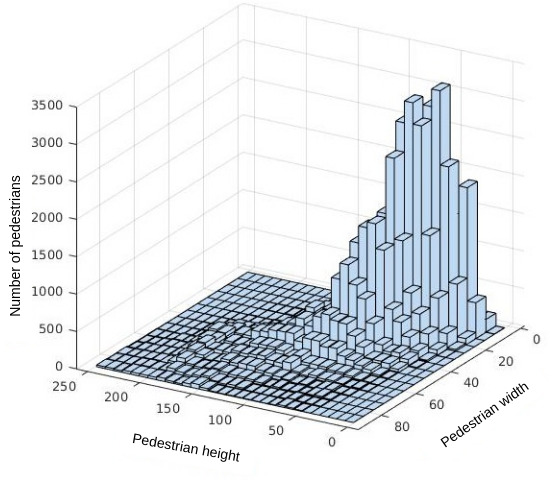
Figure 2. Histogram of height and width of bounding boxes of pedestrians of the present sample database

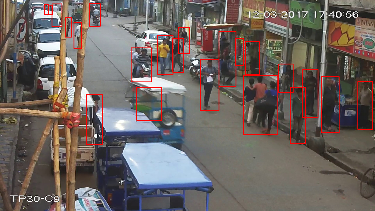
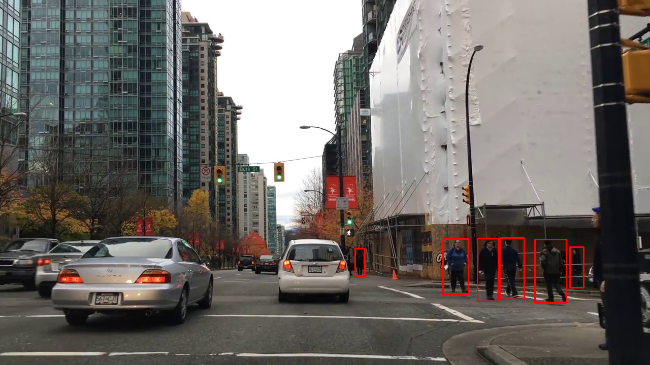
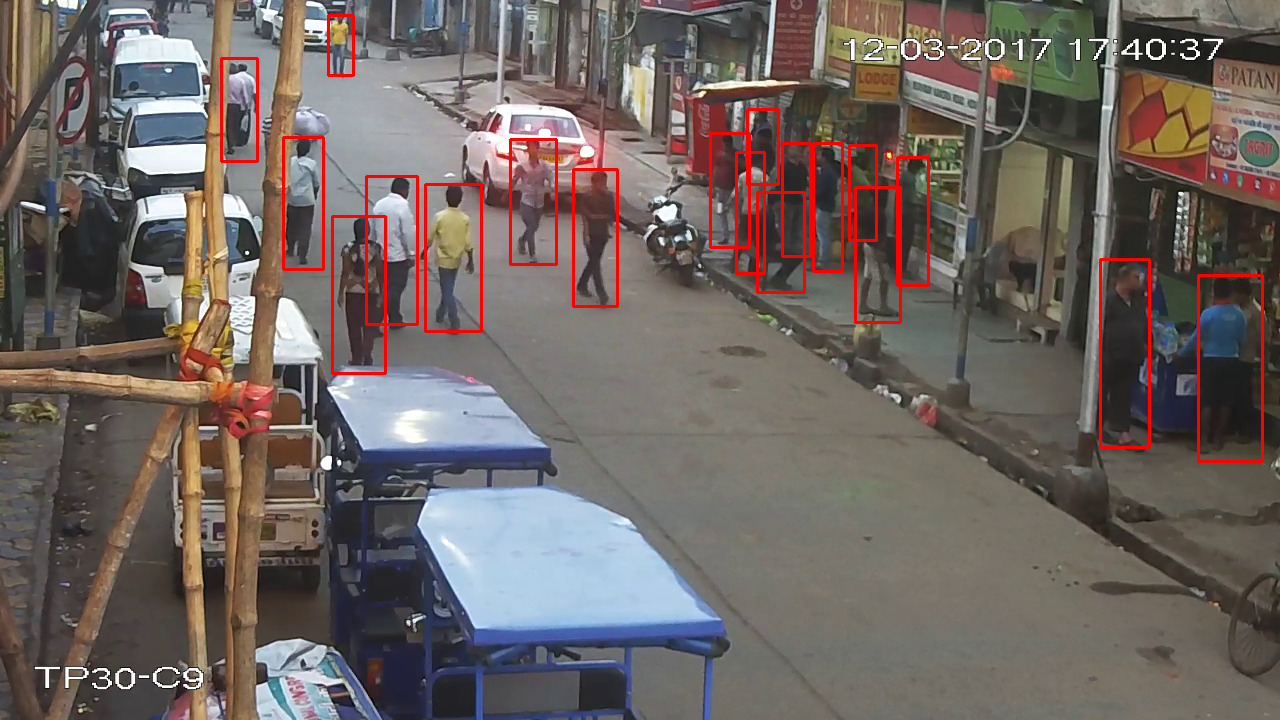
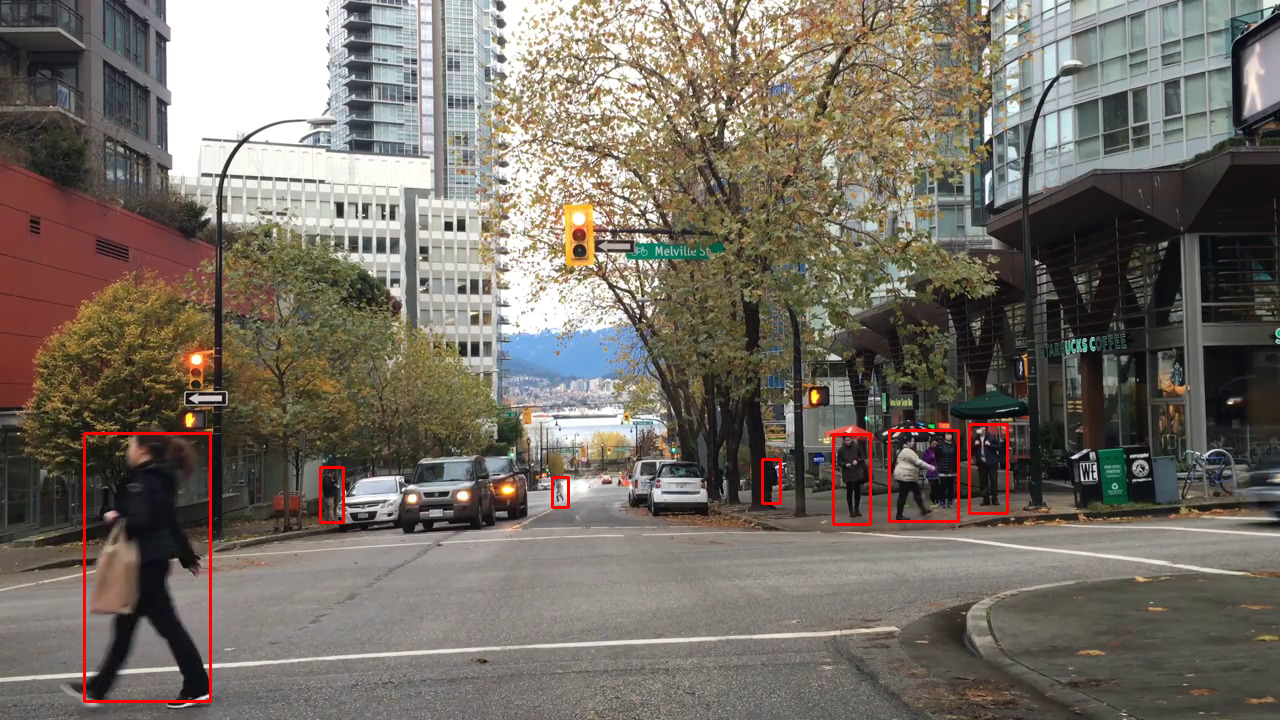
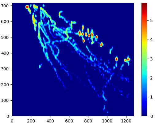
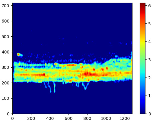
Figure 3. Two columns shows two different camera angles, traffic conditions and pedestrian variations. Corresponding distribution heat map is given in last row of each column.

The resolution of the video frames of CPD is $640\times 480$ pixels whereas the same of ISIPD is $1280\times 720$ pixels. We have kept the resolution higher to facilitate the detection of smaller pedestrian figures. Several video segments captured by different cameras fitted in different vehicles and a number of traffic surveillance cameras under normal traffic conditions of different urban areas of India, North America and Germany have been used to develop this new dataset. The video segments are so selected that various possible characteristics of the crowd or pedestrians get represented in this new dataset. On the contrary, the existing CPD consists of approximately 10 hours of continuous video taken from a particular vehicle driving through regular traffic of certain urban environment. There are video frames in the CPD which do not have any pedestrian. On the other hand, each video frame of ISIPD has at least one pedestrian. The pedestrian bounding boxes of each image of ISIPD has been manually annotated using a tailor made software tool. In Fig. 3, two different traffic scenario is presented along with the heat-map of log-normalized distribution of the center positions of pedestrians.

The training set of existing CPD consists of 128K images and 192K pedestrian bounding boxes. The development of new ISIPD is aimed at capturing more variations in the training samples towards efficient training of the network. A few pedestrian image samples of ISIPD are shown in Fig. 4.

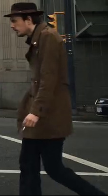
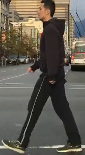
Figure 4. A few pedestrian samples of ISIPD representing its wide variations with respect to clothing, lighting condition, pose, resolution etc.

Volumes of training sets of different sample databases used in the present study are shown in Table 1.

Table 1. Training set size of different sample datasets used in the present study

Dataset Name	Total Frames	BBoxs	Resolution
CPD	128K	192K	$640\times 480$
CityPersons (Zhang et al., 2017)	2.9K	19.6K	$2048\times 1024$
ISIPD	13.1K	82.3K	$1280\times 720$

4. Proposed Model

An important feature of the proposed model is its simplicity. In the proposed strategy, we first look for potential zones (Seek) where pedestrian figures may exist. Such a potential zone is an area of the frame where the following situations may occur,

• It may contain pedestrian figures of very small size (due to its distance from the camera).

• It may contain pedestrian figures of very large size (due to its proximity to the camera). A few such figures may be so large that it may be distributed over multiple adjacent regions.

• Multiple pedestrians may appear in a single region. Some of these pedestrian figures may appear connected.

Once a zone is identified as a potential one, we further scan it (using a sliding window) to compute the bounding box of each pedestrian or connected pedestrian(s) (Find). We name this architecture as Seek and You will Find (SaYwF). The advantage of this strategy is that the parts of the frame which are unlikely to have a pedestrian figure can be rejected as non-potential zone. Thus we can restrict the number of expensive sliding window operations and subsequently improve the overall FPS. The only issue that remains is the correct identification of a potential zone. Errors in this detection stage may drop the MR heavily. We have solved the problem by introducing a simple feed-forward multi-layer classifier that can distinguish between potential and non-potential zones. We term this classifier as Zone Classifier ($C_{z}$). It is based on a CNN based Inception style network (Szegedy et al., 2015) details of which have been discussed in Sec. 4.1. Training of $C_{z}$ is accomplished by dividing each training frame image in $4\times 4$ grids (as shown in Fig. 5) yielding $16$ sub-images from each frame. The annotation groundtruth is consulted to label each such sub-image. If any part of a pedestrian figure falls within a sub-image, it is considered as a positive sample and otherwise the same is treated as a negative sample. Some positive training samples are shown in Fig. 6. It may be noted that some of the positive samples contain multiple pedestrians or only a part of a pedestrian.

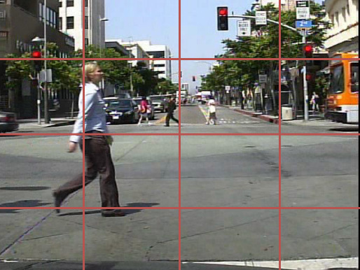
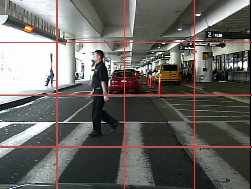
Figure 5. 4$\times$4 grid views of two original image frames. The frame to the left has eight positive sub-images while the frame to the right has three positive sub-images.

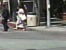
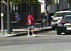
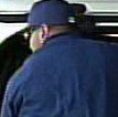
Figure 6. A few positive training samples for classifier $C_{z}$.

Once the zone classifier is ready the detection can be done in three phases. In the first phase we use ($C_{z}$) to identify an area of the frame as a potential zone. As we have no prior information about the number, size and position of pedestrian figures, we again sub divide original frame by a grid (yielding multiple sub-images). Feeding each one of the sub-image to ($C_{z}$) result confidence score of that region. Based on these scores we select a region for further processing. This is explained in Sec. 4.3.

In the second phase, we need to find the exact bounding box around each pedestrian from the potential zones suggested in phase I. To achieve this we trained another deeper binary classifier (referred as Pedestrian Classifier or $C_{p}$) based on the similar architecture as said earlier, that identifies the pedestrian and this trained classifier is fed with regions taken from a sliding window over a potential zone. Note that the sliding window size and stride are two important parameters to correctly find a pedestrian figure.

In the third phase, we used a Non-Maximum Suppression (NMS) method to reject multiple bounding box suggestions for same pedestrian and finally draw the bounding box. Instead of densely scanning all possible regions of an input video frame, we densely scan only proposed potential zones.

4.1. Modified Inception Architecture

We propose a densely connected CNN based modified Inception architecture to build a classifier. One such inception block is shown in Fig. 7. In our architecture we have appended multiple such blocks sequentially. This is illustrated in Fig. 9 and Fig. 10. A few important attributes of the inception block includes the following:

• Two filters having different orientation is used. One of them is horizontal ($1\times 3$) and the other one is vertical ($3\times 1$). Instead of using a traditional ($3\times 3$) filter, we have used these two asymmetric filters to reduce the computation time. Number of multiplications in our scheme with two filters are $6$. Whereas the same for a ($3\times 3$) filter is 9. As the computation time is proportional to number of multiplications we achieve a 1.5 times faster computation in our scheme.

• First layer of our inception block is to reduce the dimension (channels only) of the input coming from previous layers. This reduced feature map is processed by an expensive (3 $\times$3) and (5 $\times$ 5) filters followed by a max pooling layer with (4 $\times$4) with 1 stride.

• A residual connection to reuse the original context of the information from previous layer is used. This also prevents the problem of vanishing or exploding gradient during gradient descent optimization as mentioned in (He et al., 2016). It also reduces the time to convergence than the traditional Inception network (Huang et al., 2017).

• Smaller filters ($1\times 3$) are used prior to larger filters ($3\times 3$) as smaller filters preserves the special context and larger filters extract higher dimensional features.

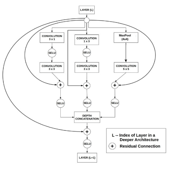
Figure 7. Inception style CNN architecture

We incorporated Batch Normalization (BN) layer as a regularizer (Ioffe and Szegedy, 2015) which helps for faster learning. In the original paper (He et al., 2016), He et al. applied BN in $Convolution\rightarrow BN\rightarrow ReLU$ order.

Consider x is feature vector, W is weight matrix and b is the bias,

$$z\leftarrow ReLU(BN(Wx+b))$$

(1) $$y\leftarrow BN(Wx+b)$$

$$E[z]=E[ReLU(y)]>E[y]=0,$$

(2) $$Var[z]=var[Relu(y)]<var[y]=1$$

But the variance and mean of normalized output from $BN$ layer is altered by the ReLU (Krizhevsky et al., 2012) operation as ReLU function transforms all the negative value to positive. For this reason, In our architecture we have used Scaled Exponential Linear Unit (SELU) (Klambauer et al., 2017) activation function (refer to Eqn. 3) after Convolution to avoid this inconsistency.

(3) $$SELU(x)=\lambda\begin{cases}x&\text{if $x>0$}\\ \alpha^{x}-\alpha&\text{if $x\leq 0$}\end{cases}$$

where $\lambda$ and $\alpha$ are fixed parameters. The negative and positive value output of the Convolution layer remain same in this SELU activation function to control the zero mean and unit variance. It helps for faster learning because of approximately zero mean and avoid the vanishing/exploding gradient problem.

4.2. Phase I: Seek if any pedestrian is there

As mentioned earlier this phase consists of a binary classifier ($C_{z}$) that can classify a region of the image as potential zone. We have used our modified Inception block to build this classifier. This is shown in Fig. 9. Size of the input RGB color image is $64\times 64$. Details of the classifier network is described bellow.

The frame is divided into $16$ regions by a $4\times 4$ grid. Each one of these regions yields a confidence score as a potential zone when given as input to our zone classifier $C_{z}$. If a region is not a potential zone (there are no pedestrian or part of pedestrian in this region) it is discarded, otherwise it is marked by a special flag and passed to Phase II. We have sampled 100K positive images and 180k negative images to train $C_{z}$.

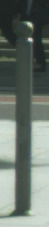
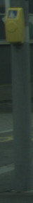
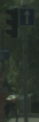
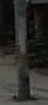
Figure 8. A few hard-negative training samples.

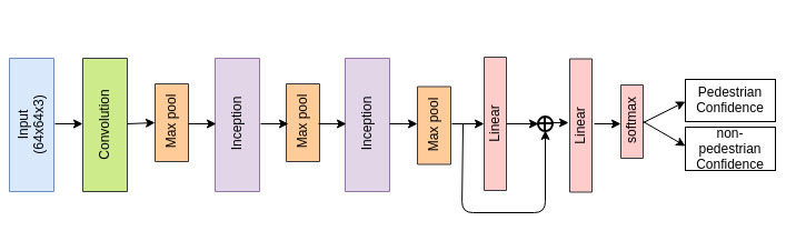
Figure 9. Potential Zone Classifier $C_{z}$

Table 2. Details of the Zone Classifier.

Type	Patch size/stride	Output Size	# $1\times 1$ residual	#$1\times 3$	#$3\times 3$	#$1\times 1$ residual	#$3\times 1$	#$3\times 3$	#residual $1\times 1$	$5\times 5$	bridge residual	params
convolution	3$\times$3/2	$32\times 32$/32	-	-	-	-	-	-	-	-	-	896
max Pool	4$\times$4/2	16$\times$16/32	-	-	-	-	-	-	-	-	-	-
inception	-	16$\times$16/64	16	8	16	16	8	16	32	32	64	33744
max Pool	4$\times$4/2	8$\times$8/64	-	-	-	-	-	-	-	-	-	-
inception	-	8$\times$8/96	32	16	32	32	16	32	64	64	128	79168
max Pool	4$\times$4/2	4$\times$4/96	-	-	-	-	-	-	-	-	-	-
linear	-	128	-	-	-	-	-	-	-	-	-	196736
residual	-	128	-	-	-	-	-	-	-	-	-	196736
linear	-	2	-	-	-	-	-	-	-	-	-	514
softmax	-	2	-	-	-	-	-	-	-	-	-	-

Table 3. Details of the Pedestrian Classifier.

Type	Patch size/stride	Output Size	# $1\times 1$ residual	#$1\times 3$	$\#3\times 3$	#$1\times 1$ residual	#$3\times 1$	#$3\times 3$	#residual $1\times 1$	$5\times 5$	bridge residual	params
convolution	3$\times$3/1	64$\times$64/32	-	-	-	-	-	-	-	-	-	896
max Pool	4$\times$4/2	32$\times$32/32	-	-	-	-	-	-	-	-	-	-
inception	-	32$\times$32/64	32	16	32	32	16	32	16	16	64	24080
max Pool	4$\times$4/2	16$\times$16/64	-	-	-	-	-	-	-	-	-	-
inception	-	16$\times$16/128	48	32	48	48	32	48	32	32	128	91584
inception	-	16$\times$16/128	48	32	48	48	32	48	32	32	128	111040
max Pool	4$\times$4/2	8$\times$8/128	-	-	-	-	-	-	-	-	-	-
inception	-	8$\times$8/200	80	40	80	80	40	80	40	40	200	226320
inception	-	8$\times$8/200	80	40	80	80	40	80	40	40	200	226320
max Pool	4x4/2	4x4/200	-	-	-	-	-	-	-	-	-	-
linear	-	512	-	-	-	-	-	-	-	-	-	1638912
linear	-	256	-	-	-	-	-	-	-	-	-	131328
residual	-	256	-	-	-	-	-	-	-	-	-	819456
linear	-	2	-	-	-	-	-	-	-	-	-	514
softmax	-	2	-	-	-	-	-	-	-	-	-	-

4.3. Phase II: Find where are the pedestrians

The classifier $C_{z}$ of Phase I has already provided a collection of potential zones $Z_{1},Z_{2},\ldots$. Now, a sliding window of size 16 $\times$ 16 is densely moved (small step size) over each $Z_{i}$. Use of a larger step size should plummet the MR while it may cause increased FPS. Here, a step size of 5 has been empirically selected. The effect of step size on MR and FPS has been discussed in Sec. 5. The region or area cropped by the sliding window is re-scaled to feed the same as input to the pedestrian detection classifier $C_{p}$ (Fig. 10).

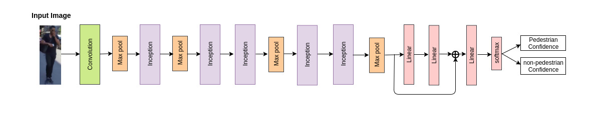
Figure 10. Pedestrian Detection Classifier $C_{p}$

A detail configuration of the classification model is given in Table 3. Total number of parameters of our deep architecture is $\sim$3.3 Million which is much less than Deep Network Cascades (DNC) which consists of $\sim$50 million parameters. The processing as done in Phase I and II are shown graphically in Fig. 11.

4.4. Phase III: One and only one

The image region covered in one sliding window position within a potential zone is processed by the classifier ($C_{p}$) trained previously (refer to Sec. 4.3). When the scan is complete we get a heatmap of the frame denoting existence of pedestrians (detection window). It should be noted that after the sliding window completes the scan of a single potential zone. We may get multiple overlapping detection windows inside a potential zone for a single pedestrian position. Thus redundant bounding boxes are eliminated by Non-Maximum Suppression (NMS). It is done by not considering image regions (corresponds to different sliding window positions) that are overlapping with some detection window by 50% IOU (Intersection over Union).

Now we face an interesting situation when a pedestrian figure is distributed over multiple adjacent potential zones. One such scenario is shown in Fig. 12, where $C_{z}$ has detected $Z_{1}$, $Z_{2}$, $Z_{3}$ and $Z_{4}$ as potential zones. $C_{p}$ has estimated the bounding boxes (say, $W_{1}$, $W_{2}$, $W_{3}$ and $W_{4}$) for individual parts of the pedestrian lying in each of these zones. Our task is to identify the occurrence of a similar situation and merge the corresponding bounding boxes. Towards the same, we first detect pairs of adjacent potential zones. For each such pair, we run a sliding window ($S_{w}$) of size $32\times 32$ with its center on the common boundary. $S_{w}$ is resized to $64\times 64$ to feed it to the classifier $C_{p}$. If $S_{w}$ is classified as pedestrian, then we further compute its overlaps with pedestrian bounding boxes (if any) of both the adjacent zones. If at least one such $S_{w}$ has significant overlap with a pedestrian bounding box lying in each of the two zones, then the corresponding pedestrian bounding boxes of the two zones are merged.

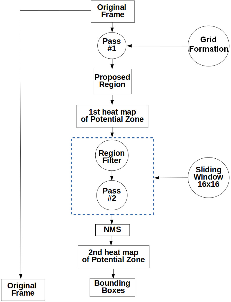
Figure 11. Flow chart of the proposed method.

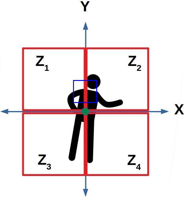
Figure 12. A single pedestrian figure is distributed over four adjacent regions each of which has been identified as a potential zone by the classifier $C_{z}$. The sliding window (blue) centered on the boundary of $Z_{1}$ and $Z_{2}$ has significant overlap with pedestrian bounding boxes of both of the two zones.

5. Experimental Results

There are many interesting aspects related to pedestrian detection problem using CNN based deep learning methods. Some of them include (i) the trade off between FPS and MR, (ii) effect of stride size on FPS and MR, (iii) effect of selection of training and test sets etc. We have explored quite a few of these aspects through experiments.

As mentioned earlier, our model uses two classifiers $C_{z}$ (Fig. 9) and $C_{p}$ (Fig. 10). These two were trained using training sets $D_{z}$ and $D_{p}$ respectively which were formed from training samples of three datasets viz., CPD, CityPersons and ISIPD. Training and test set details including the numbers of positive and negative samples have been provided in Table 4. Training was executed on a system consisting of three Nvidia Tesla P6 GPU and for each mini batch of size 2048, it takes  700 milliseconds. Training is continued until training loss is saturated.

Table 4. Dataset ($D_{z}$ and $D_{p}$) Details.

Model	Training set		Test set
Type of Sample	Positive	Negative	Positive	Negative
$D_{z}$	100k	180k	50k	50k
$D_{p}$	210k	1.2 million	90k	90k

The performance of the proposed end-to-end pedestrian detection system has been measured based on MR and FPS. MR is computed by comparing the IOU of bounding boxes from original annotated image with the predicted bounding boxes. If the overlap between actual and predicted bounding box is more than 50% then we consider this as a hit. Miss can occur if either we positively detect a region with out pedestrian or fail to detect a region with pedestrian. Miss rate is computed based on these outcome. Our model can process 20 frames on Nvidia Titan XP GPU. To compare the performance of our model is compared with some existing state of the art deep CNN based architectures. Note that only those models that can process at least 10 frames per second (10 FPS and above) are chosen.

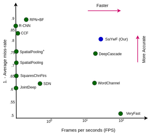
Figure 13. Performance of different model on Caltech Pedestrian Dataset.

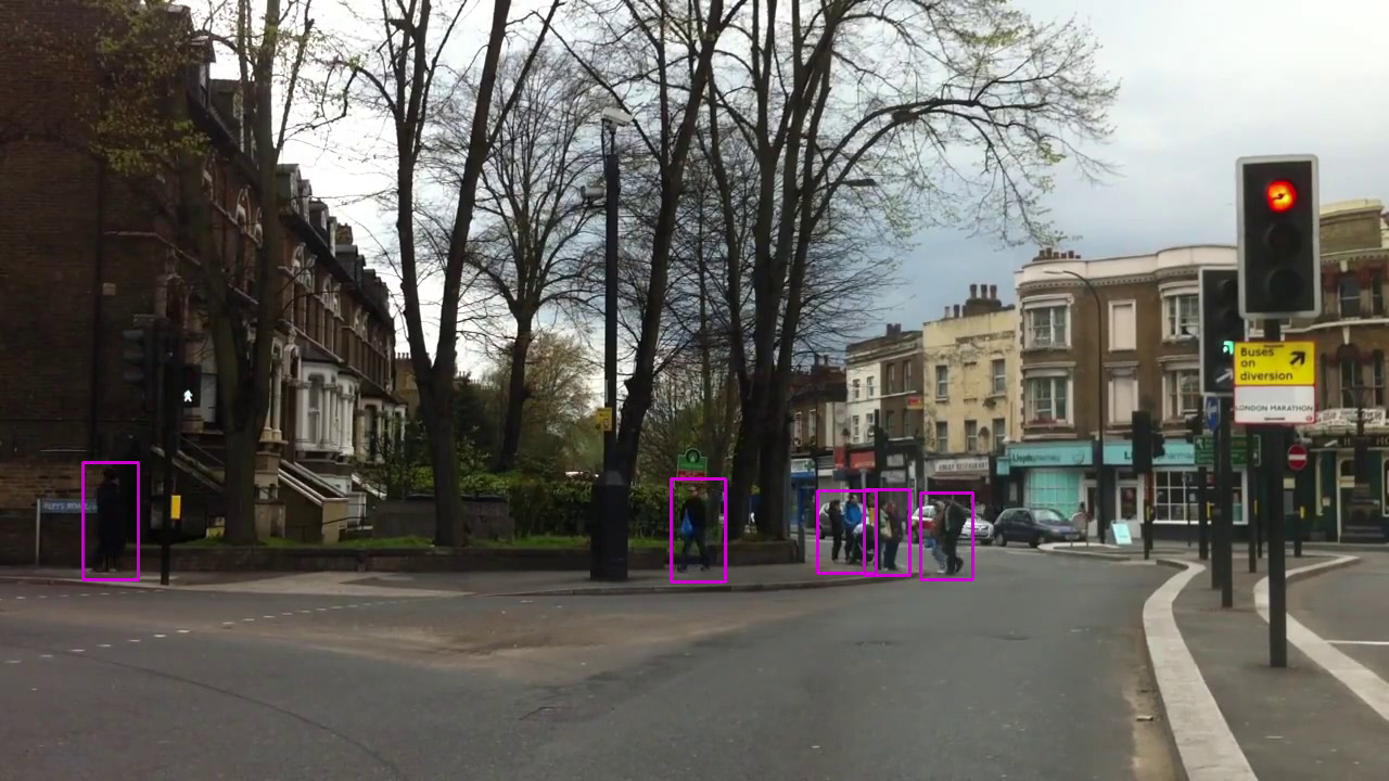
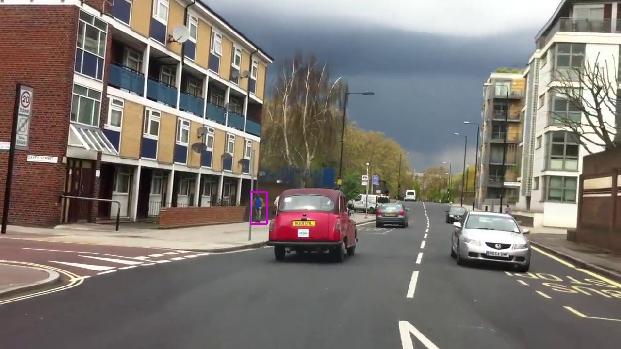
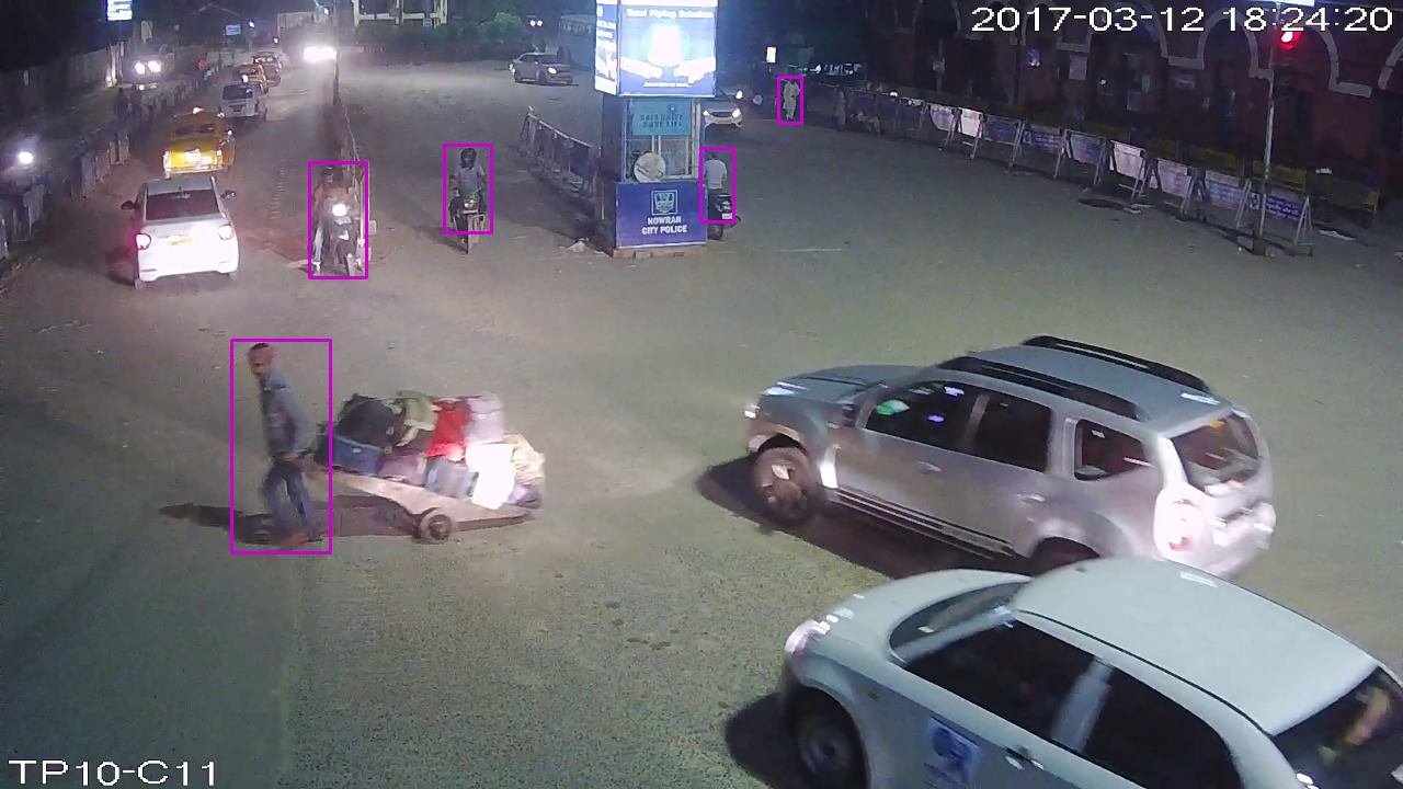
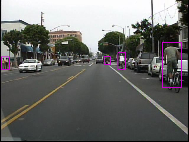
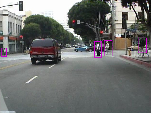
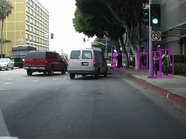
Figure 14. Some Output Image Generated from SaYwF.

The outcome of our experimentation (shown in Table 6.) clearly suggests that the proposed model SaYwF obtained better accuracy. Also, its processing speed (FPS) is very close to the DNC benchmark. On the other hand, SaYwF did not perform up to the mark in terms of FPS for the newly created dataset as the video resolution of the new dataset is nearly double to that of CPD. We plan to do studies to improve the performance of our model for high resolution video processing.

As FPS depends on the stride of the sliding window we also performed several experiments to observe the variation of FPS against stride and also variation of FPS against MR to justify the FPS MR trade-off. This is illustrated in Fig. 15 where MR and FPS are normalized in range (0,1). Note that the distance of pedestrian from camera is categorized in three classes and they are Near, Medium and Far.

As mentioned earlier, we have opted for SELU activation function over RELU, a more popular variety. This choice has been prompted by extensive experimentation and here, in Fig. 16, we have shown the comparative performance in terms of network loss on the combined training sets of the three databases used in the present study.

Another set of experiments has been performed with different train set and test set combinations. We have used negative mining to increase the volume of the train set of previously specified binary classifiers. Here, we have taken false negative from SaYwF output and included them as negative samples in the training set to improve overall accuracy. These results are provided in Tables 5 and 6. Also, the recall values of both the classifiers are provided in Table 7.

Table 5. MR of different models corresponding to different combinations of train and test sets

Model	Test $\downarrow$	Train
		CPD	CityPersons	ISIPD
DNC	CPD	39.37	41.77	35.53
	CityPersons	43.19	44.92	33.79
	ISIPD	45.48	48.67	33.43
googleNet	CPD	37.49	38.93	35.53
	CityPersons	40.93	42.63	31.08
	ISIPD	43.51	46.18	31.58
SaYwF(Our)	CPD	37.28	38.43	32.31
	CityPersons	39.58	40.52	29.31
	ISIPD	42.98	44.73	29.93

Table 6. Experimental results (MR and FPS) of different models trained using CPD, CityPersons, ISIPD datasets

Architecture	Dataset
	CPD		City Person		ISIPD
	MR	FPS	MR	FPS	MR	FPS
DNC	25.39	15	28.77	7	31.43	10
googleNet	21.49	21	25.93	10	28.58	13
SaYwF	18.11	20	23.78	8	27.33	11

Table 7. Recall at different stages of classification.

Phase	Pedestrian Recall
$C_{z}$ (Phase I)	93.04
$C_{p}$ (Phase II) and NMS (Phase III)	88.01

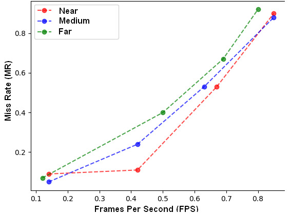
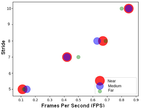
Figure 15. Dependency between MR, FPS and stride size.

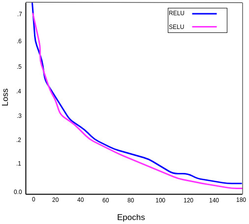
Figure 16. Comparison of losses provided by RELU vs. SELU.

Here it may be noted that the first stage eliminates a large number of candidate windows (non-potential zones) for improving the processing time. In this phase one can also use some non-CNN based algorithms like exhaustive search (Harzallah et al., 2009), selective search (Uijlings et al., 2013) or BPM (Felzenszwalb et al., 2010) techniques, but our experiment shows that $C_{z}$ classifier based approach is both accurate and faster. In the first stage (that uses the $C_{z}$ network) it takes 7.2 ms to detect possible potential zones among 16 regions of an input frame (refer to Sec 4.2). The second stage (with $C_{p}$ classifier) takes around 40.7 ms to predict all bounding boxes. Overall execution time is 52 ms (including NMS) for a 640 $\times$ 480 frame consequently yielding 20 FPS processing time.

6. Conclusions

Considering real life applications of pedestrian detection systems, its execution in real time with high accuracy is crucial. However, there is hardly any available system that is optimized with respect to both execution speed (FPS) and detection accuracy (measured in terms of miss rate or MR). In view of the same we have designed the proposed Seek and You will Find (SaYwF) architecture. It first looks (Seek) for potential zones of a video frame where a pedestrian or its part may exist. Next, it identifies (You will Find) the part of such a zone where the pedestrian or its part actually appears. An instance of a pedestrian may lie in one or more such neighbouring regions. The final non-maximum suppression stage combines the parts of these regions to obtain the bounding box of the instance of a pedestrian. For effective training of the proposed model we have developed a new sample dataset (ISIPD) to capture wide variations among the training samples. This database will be distributed freely for academic research purposes.

References

- (1)
- Alonso et al. (2007) Ignacio Parra Alonso, David Fernández Llorca, Miguel Ángel Sotelo, Luis M Bergasa, Pedro Revenga de Toro, Jess Nuevo, Manuel Ocaña, and Miguel Ángel García Garrido. 2007. Combination of feature extraction methods for SVM pedestrian detection. IEEE Transactions on Intelligent Transportation Systems 8, 2 (2007), 292–307.
- Angelova et al. (2015) Anelia Angelova, Alex Krizhevsky, Vincent Vanhoucke, Abhijit S Ogale, and Dave Ferguson. 2015. Real-Time Pedestrian Detection with Deep Network Cascades.. In BMVC, Vol. 2. 4.
- Appel et al. (2013) Ron Appel, Thomas Fuchs, Piotr Dollár, and Pietro Perona. 2013. Quickly boosting decision trees–pruning underachieving features early. In International conference on machine learning. 594–602.
- Benenson et al. (2012) Rodrigo Benenson, Markus Mathias, Radu Timofte, and Luc Van Gool. 2012. Pedestrian detection at 100 frames per second. In Computer Vision and Pattern Recognition (CVPR), 2012 IEEE Conference on. IEEE, 2903–2910.
- Dalal and Triggs (2005) Navneet Dalal and Bill Triggs. 2005. Histograms of oriented gradients for human detection. In Computer Vision and Pattern Recognition, 2005. CVPR 2005. IEEE Computer Society Conference on, Vol. 1. IEEE, 886–893.
- Ding and Xiao (2012) Yuanyuan Ding and Jing Xiao. 2012. Contextual boost for pedestrian detection. In Computer Vision and Pattern Recognition (CVPR), 2012 IEEE Conference on. IEEE, 2895–2902.
- Dollár et al. (2009) Piotr Dollár, Christian Wojek, Bernt Schiele, and Pietro Perona. 2009. Pedestrian detection: A benchmark. In IEEE conference on computer vision and pattern recognition, 2009. CVPR 2009. IEEE Conference on. IEEE, 304–311.
- Dollar et al. (2012) Piotr Dollar, Christian Wojek, Bernt Schiele, and Pietro Perona. 2012. Pedestrian detection: An evaluation of the state of the art. IEEE transactions on pattern analysis and machine intelligence 34, 4 (2012), 743–761.
- Enzweiler and Gavrila (2008) Markus Enzweiler and Dariu M Gavrila. 2008. Monocular pedestrian detection: Survey and experiments. IEEE Transactions on Pattern Analysis & Machine Intelligence 12 (2008), 2179–2195.
- Ess et al. (2008) Andreas Ess, Bastian Leibe, Konrad Schindler, and Luc Van Gool. 2008. A mobile vision system for robust multi-person tracking. In Computer Vision and Pattern Recognition, 2008. CVPR 2008. IEEE Conference on. IEEE, 1–8.
- Felzenszwalb et al. (2010) Pedro F Felzenszwalb, Ross B Girshick, David McAllester, and Deva Ramanan. 2010. Object detection with discriminatively trained part-based models. IEEE transactions on pattern analysis and machine intelligence 32, 9 (2010), 1627–1645.
- Freund (2001) Yoav Freund. 2001. An adaptive version of the boost by majority algorithm. Machine learning 43, 3 (2001), 293–318.
- Geiger et al. (2012) Andreas Geiger, Philip Lenz, and Raquel Urtasun. 2012. Are we ready for autonomous driving? the kitti vision benchmark suite. In Computer Vision and Pattern Recognition (CVPR), 2012 IEEE Conference on. IEEE, 3354–3361.
- Harzallah et al. (2009) Hedi Harzallah, Frédéric Jurie, and Cordelia Schmid. 2009. Combining efficient object localization and image classification. In Computer Vision, 2009 IEEE 12th International Conference on. IEEE, 237–244.
- He et al. (2016) Kaiming He, Xiangyu Zhang, Shaoqing Ren, and Jian Sun. 2016. Deep residual learning for image recognition. In Proceedings of the IEEE conference on computer vision and pattern recognition. 770–778.
- Huang et al. (2017) Gao Huang, Zhuang Liu, Kilian Q Weinberger, and Laurens van der Maaten. 2017. Densely connected convolutional networks. In Proceedings of the IEEE conference on computer vision and pattern recognition, Vol. 1. 3.
- Ioffe and Szegedy (2015) Sergey Ioffe and Christian Szegedy. 2015. Batch normalization: Accelerating deep network training by reducing internal covariate shift. arXiv preprint arXiv:1502.03167 (2015).
- Klambauer et al. (2017) Günter Klambauer, Thomas Unterthiner, Andreas Mayr, and Sepp Hochreiter. 2017. Self-normalizing neural networks. In Advances in Neural Information Processing Systems. 972–981.
- Krizhevsky et al. (2012) Alex Krizhevsky, Ilya Sutskever, and Geoffrey E Hinton. 2012. Imagenet classification with deep convolutional neural networks. In Advances in neural information processing systems. 1097–1105.
- Luo et al. (2014) Ping Luo, Yonglong Tian, Xiaogang Wang, and Xiaoou Tang. 2014. Switchable deep network for pedestrian detection. In Proceedings of the IEEE Conference on Computer Vision and Pattern Recognition. 899–906.
- Luo et al. (2013) Ping Luo, Xiaogang Wang, and Xiaoou Tang. 2013. Pedestrian parsing via deep decompositional network. In Proceedings of the IEEE international conference on computer vision. 2648–2655.
- Papageorgiou and Poggio (2000) Constantine Papageorgiou and Tomaso Poggio. 2000. A trainable system for object detection. International journal of computer vision 38, 1 (2000), 15–33.
- Ren et al. (2015) Shaoqing Ren, Kaiming He, Ross Girshick, and Jian Sun. 2015. Faster r-cnn: Towards real-time object detection with region proposal networks. In Advances in neural information processing systems. 91–99.
- Szegedy et al. (2015) Christian Szegedy, Wei Liu, Yangqing Jia, Pierre Sermanet, Scott Reed, Dragomir Anguelov, Dumitru Erhan, Vincent Vanhoucke, and Andrew Rabinovich. 2015. Going Deeper With Convolutions. In The IEEE Conference on Computer Vision and Pattern Recognition (CVPR).
- Tuzel et al. (2008) Oncel Tuzel, Fatih Porikli, and Peter Meer. 2008. Pedestrian detection via classification on riemannian manifolds. IEEE transactions on pattern analysis and machine intelligence 30, 10 (2008), 1713–1727.
- Uijlings et al. (2013) Jasper RR Uijlings, Koen EA Van De Sande, Theo Gevers, and Arnold WM Smeulders. 2013. Selective search for object recognition. International journal of computer vision 104, 2 (2013), 154–171.
- Xu et al. (2005) Fengliang Xu, Xia Liu, and Kikuo Fujimura. 2005. Pedestrian detection and tracking with night vision. IEEE Transactions on Intelligent Transportation Systems 6, 1 (2005), 63–71.
- Zhang et al. (2016) Liliang Zhang, Liang Lin, Xiaodan Liang, and Kaiming He. 2016. Is faster r-cnn doing well for pedestrian detection?. In European Conference on Computer Vision. Springer, 443–457.
- Zhang et al. (2017) Shanshan Zhang, Rodrigo Benenson, and Bernt Schiele. 2017. Citypersons: A diverse dataset for pedestrian detection. arXiv preprint arXiv:1702.05693 (2017).