The Gor’kov and Melik-Barkhudarov correction to the mean-field critical field transition to Fulde-Ferrell-Larkin-Ovchinnikov states

Abstract

The Fulde-Ferrell-Larkin-Ovchinnikov (FFLO) states, characterized by Cooper pairs condensed at finite-momentum are, at the same time, exotic and elusive. It is partially due to the fact that the FFLO states allow superconductivity to survive even in strong magnetic fields at the mean-field level. The effects of induced interactions at zero temperature are calculated in both clean and dirty cases, and it is found that the critical field at which the quantum phase transition to an FFLO state occurs at the mean-field level is strongly suppressed in imbalanced Fermi gases. This strongly shrinks the phase space region where the FFLO state is unstable and more exotic ground state is to be found. In the presence of high level impurities, this shrinkage may destroy the FFLO state completely. Ann. Phys. (Berlin) 2020, 2000222; DOI: 10.1002/andp.202000222

I Introduction

Fermionic particles with two different spins occupying states of momenta with equal size but in opposite directions close to their common Fermi surface form Cooper pairs, when subject to a pairing interaction. This is successfully explained by the Bardeen-Cooper-Schrieffer (BCS) theory of superconductivity Bardeen et al. (1957). The presence of an imbalance between the two spin configurations prevents this mechanism, since there are now two Fermi surfaces that do not coincide so that pairing with zero total momentum for the BCS state is energetically unfavorable, as the formation of Cooper pairs implies equal densities of the two spin species Chen et al. (2007); Giorgini et al. (2008); Inguscio et al. (2007); Bloch et al. (2008).

The difficulty of BCS pairing caused by spin imbalance led to the proposal of possible energetically more favorable Fulde-Ferrell-Larkin-Ovchinnikov (FFLO) states  Fulde and Ferrell (1964); Larkin and Ovchinnikov (1965), which Bose condense into a finite momentum $\mathbf{q}$ or a pair of momenta $\pm\mathbf{q}$ (for FF and LO states, respectively). The FF state features a single-plane-wave superfluid order parameter, $\Delta_{\mathbf{R}}=\Delta e^{i\mathbf{q}\cdot\mathbf{R}}$, which has a spatially uniform amplitude. And the LO phase has a standing-wave-like order parameter, $\Delta_{\mathbf{R}}=\Delta\cos(\mathbf{q}\cdot\mathbf{R})$, which is a superposition of two counterpropagating plane waves, and is inhomogeneous in both amplitude and phase. The LO phase can be generalized to higher order crystalline states with multiple plane-wave components. While a stable FFLO state may exist in an anisotropic system Shimahara (1999, 1998) or in a lattice Samokhin and Mar’enko (2006a); Shimahara (1998); Kinnunen et al. (2018), especially in a low dimensions Koponen et al. (2008); Ptok (2017); Revelle et al. (2016), however, it has been shown that the FFLO states are intrinsically unstable in clean homogeneous three-dimensional (3D) and 2D continuum systems Wang et al. (2018). Instead, noncondensed pairing with the lowest pair energy at finite momenta is expected, which may lead to exotic ground states. Thus it is important to find the true solution where the unstable mean-field FFLO solutions exist. While this is a very difficult issue, in this paper, we aim to further constrain the phase space region where exotic pairing state may live. In particular, we find that particle-hole fluctuations help to significantly reduce the critical field transition window for the mean-field FFLO states. This also implies that the regions that otherwise have a mean-field FFLO solution should now exhibit more conventional solutions, such as polaronic normal phase Schirotzek et al. (2009); Nascimbène et al. (2009) and phase separation Shin et al. (2006); Partridge et al. (2006).

At the mean-field (MF) level, for small asymmetries between the two spin species, and at zero temperature $T$, the system persists as a BCS superfluid of zero momentum. However, when the imbalance between the two Fermi surfaces is too large, superfluid pairing is broken apart so that the system undergoes a quantum phase transition to the normal state. Therefore, for a given imbalance, there exists a lower threshold of pairing strength for the BCS pairing solution to exist. On the other hand, for a given interaction strength, there exists an upper bound for the imbalance before pairing is broken. The existence of such a transition at a critical value of the polarization was first realized by Clogston Clogston (1962) and Chandrasekhar Chandrasekhar (1962), who independently predicted the occurrence of a first-order phase transition from the superfluid to the normal state. This is known as the Clogston-Chandrasekhar (CC) limit of superfluidity, and was originally proposed in the context of conventional superconductivity.

Stability analysis based on energetic considerations reveals that the mean-field BCS solution at $T=0$ is not stable in the presence of imbalance until the system enters the Bose-Einstein condensation (BEC) regime where the gap and hence the condensation energy become large Chien et al. (2006); Pao et al. (2006); Chen et al. (2006); Sheehy and Radzihovsky (2006). Indeed, the momentum of the minority fermions would have to be lifted up to match that of their majority partners, but the energy cost is larger than the condensation energy gain when the pairing gap is small. As a consequence, thermal smearing of the Fermi surfaces leads to possible intermediate temperature superfluidity, at both the mean-field level and with fluctuations included Chien et al. (2006).

Theoretical investigations with ultracold imbalanced Fermi gases, where the numbers of atoms in the two spin states are different, have predicted that the first order transition between the superfluid at equal spin population and the imbalanced normal mixture brings about a phase separation between coexisting normal and superfluid phases Bedaque et al. (2003); Caldas (2004). Recent experiments of Fermi gases in a trap using tomographic techniques have found a sharp separation between a superfluid core at the trap center and a partially polarized normal phase outside the core Shin et al. (2006); Partridge et al. (2006). So far, the exploration of a two-component Fermi gas with imbalanced populations remains a current and active area of research in the field of ultracold atoms in both theory Giorgini et al. (2008); Radzihovsky and Sheehy (2010); Chevy and Mora (2010); Zwerger (2012) and experiment Zwierlein et al. (2006); Partridge et al. (2006); Nascimbène et al. (2010); Navon et al. (2010); Nascimbène et al. (2011), which gives to this field the unprecedented opportunity for mimicking and simulating condensed matter systems Lewenstein et al. (2007); Osterloh et al. (2002). Particularly, population imbalance in atomic Fermi gases can access the full range between 0 and 100%, making it an ideal platform for studying the FFLO physics.

The FFLO superfluid state was proposed independently by Fulde and Ferrell Fulde and Ferrell (1964), and Larkin and Ovchinnikov Larkin and Ovchinnikov (1965), to address the possibility for the Cooper pairs in an $s$-wave superconductor in the presence of a Fermi surface mismatch caused by a Zeeman field to have a non-zero total momentum $\vec{q}$, with a spatially modulated superfluid order parameter. In this intriguing pairing mechanism, the superfluidity “perseveres” in the form of an FFLO state, with a spatial modulation of the phase and amplitude of the order parameter for the FF and LO states, respectively. In the last 55 years many groups have tried to find the FFLO phase experimentally, and some have found only indirect signatures as, for example, in the heavy fermion superconductor CeCoIn₅ Bianchi et al. (2003); Radovan et al. (2003); Kenzelmann et al. (2008); Kumagai et al. (2006); Koutroulakis et al. (2010); Tokiwa et al. (2012); Kim et al. (2016); Hatakeyama and Ikeda (2015), organic superconductors Mayaffre et al. (2014); Koutroulakis et al. (2010); Varelogiannis (2002); Lortz et al. (2007); Yonezawa et al. (2008); Bergk et al. (2011); Coniglio et al. (2011); Singleton et al. (2000); Agosta et al. (2017); Wosnitza (2018); Agosta (2018); Sugiura et al. (2019), as well as iron-based superconductors Ptok and Crivelli (2013); Cho et al. (2011, 2017). Theoretical studies have found that the FFLO states become unstable in various situations Samokhin and Mar’enko (2006b); Radzihovsky and Vishwanath (2009); Radzihovsky (2011). In particular, it is shown in Ref. Wang et al. (2018) that due to the inevitable pairing fluctuations (including both amplitude and phase), the FFLO states are intrinsically unstable in isotropic 3D and 2D systems, and thus exotic pairing state may emerge.

So far, the true stable solution is still unknown, where the above mean-field FFLO solution is stable against phase separation but unstable due to pairing fluctuations. As a first step, in the present paper, we consider the contributions of particle-hole fluctuations and study their effect on the relevant phases.

It has been known that particle-hole fluctuations may have a strong effect in the solution of the superfluid transition temperature $T_{\text{c}}$ in the BCS–BEC crossover Chen et al. (2005); Chen (2016). Namely, there is a change in the coupling of the interaction due to screening of the interspecies (or induced) interaction, known as the Gor’kov and Melik-Barkhudarov (GMB) correction Gor’kov and Melik-Barkhudarov (1961). On the BEC side of the unitarity, where the two-body scattering length diverges , fluctuations in the pairing channel are dominant, while the GMB fluctuations become weaker towards the BEC side and usually is taken as vanishing in this region due to the disappearance of the Fermi surface.

The effect of induced interactions was first considered by Gor’kov and Melik-Barkhudarov, who found that in a dilute 3D balanced spin-$1/2$ Fermi gas the (overestimated) MF transition temperature is suppressed by a factor $(4e)^{1/3}\approx 2.2$ Gor’kov and Melik-Barkhudarov (1961).

Quite generally, the calculation of the GMB correction has been restricted to the balanced case, with the Zeeman field $h=(\mu_{\uparrow}-\mu_{\downarrow})/2=0$, where $\mu_{\uparrow}$ and $\mu_{\downarrow}$ are the chemical potential of the spin-up and spin-down fermions, respectively. Previous investigations with $h\neq 0$ were focused on the effects of the induced interactions on the tricritical point $(p_{\text{t}},T_{\text{t}}/T_{\text{F}})$ of imbalanced Fermi gases in 3D Yu and Yin (2010) and 2D Resende et al. (2012). Here $p_{\text{t}}$ and $T_{\text{t}}$ are the polarization and the temperature at the tricritical point, and $T_{\text{F}}$ is the Fermi temperature. (And we define Fermi energy and Fermi momentum via $E_{\text{F}}=k_{\text{B}}T_{\text{F}}=\hbar^{2}k_{\text{F}}^{2}/2m$). More sophisticated calculations involving self-consistent feedback effect from both particle-particle and particle-hole channels can be found in Ref. Chen (2016).

Another important factor that has a strong impact on the superfluid phase is disorder and impurity scattering. The effects of disorder on an FFLO state have been investigated in $s$- Aslamazov (1959); Takada (1970); Bulaevskii and Guseinov (1976); Agterberg and Yang (2001); Ikeda (2010); Cui and Yang (2008) and $d$-wave Agterberg and Yang (2001); Adachi and Ikeda (2003); Wang et al. (2007); Vorontsov et al. (2008); Yanase (2009); Datta et al. (2019) superconductors. While weak nonmagnetic impurities have been benign to $s$-wave BCS superconductors a la the Anderson’s theorem Anderson (1959), they may suppress or destroy an FFLO state Ptok (2010); Cui and Yang (2008).

In this paper, we investigate at the mean-field level the effects of the GMB correction on the FFLO transition that may occur in Fermi gases with imbalanced spin populations, in the clean limit and in the presence of nonmagnetic impurities. We study the continuous phase transition that is triggered by an increase in the chemical potential imbalance $h$, in homogeneous 3D systems. We find the GMB correction to the critical chemical potential imbalance $h_{\text{s}}$ responsible for the phase transitions from the partially polarized (PP) FFLO phase to a fully polarized (FP) normal state. In the presence of high level impurities, we show that short lifetimes necessarily further decrease $h_{\text{s}}$ and, consequently, reduce or even completely destroy the predicted FFLO region of existence. To our knowledge, this is the first time that the GMB correction is considered in the context of FFLO physics.

The paper is organized as follows. In Sec. II we first calculate the generalized pair susceptibility in the clean case, associated with the onset of the instability of the PP normal phase. In Sec. III we obtain the induced interactions and find its effects on the critical chemical potential imbalance $h_{\text{s}}$ which sets the transition to the FFLO phase. In Sec. IV we show how the GMB correction further reduces the FFLO window in the presence of nonmagnetic impurities. Finally, we conclude in Sec. VI.

II The Intermediate Normal-Mixed Phase

We consider a generic system of fermions characterized by an effective, short range pairing interaction $-g$, (where $g>0$), with grand canonical Hamiltonian in momentum space Chen et al. (1999, 2007)

$$H = \sum_{\mathbf{k}\sigma}\xi_{\mathbf{k}\sigma}c^{{\dagger}}_{\mathbf{k}\sigma}c^{\ }_{\mathbf{k}\sigma}$$ (1)

$$-g\sum_{\mathbf{k}\mathbf{k}^{\prime}\mathbf{q}}c^{{\dagger}}_{\mathbf{k}+\mathbf{q}/2\uparrow}c^{{\dagger}}_{-\mathbf{k}+\mathbf{q}/2\downarrow}c^{\ }_{-\mathbf{k}^{\prime}+\mathbf{q}/2\downarrow}c^{\ }_{\mathbf{k}^{\prime}+\mathbf{q}/2\uparrow},$$

where the bare dispersion $\xi_{\mathbf{k}\sigma}=\epsilon_{\mathbf{k}}-\mu_{\sigma}=\mathbf{k}^{2}/2m-\mu_{\sigma}$, and $\sigma=\uparrow,\downarrow$ is the spin index. Here $c^{\dagger}$ ($c$) is the fermion creation (annihilation) operator, and we have set the system volume to unity. We shall also take the natural units, $\hbar=k_{\text{B}}=1$. The average chemical potential $\mu=(\mu_{\uparrow}+\mu_{\downarrow})/2$. The population imbalance is defined as the relative spin density difference, $p=(n_{\uparrow}-n_{\downarrow})/(n_{\uparrow}+n_{\downarrow})$. At the mean-field level, the reduced Hamiltonian for one-plane-wave FFLO state with pairing between $\mathbf{k}$ and $-\mathbf{k}+\mathbf{q}$ states is given by He et al. (2007)

$$H^{\text{MF}} = \sum_{\mathbf{k}}\Big{\{}\xi_{\mathbf{k}\uparrow}c_{\mathbf{k}\uparrow}^{{\dagger}}c_{\mathbf{k}\uparrow}+\xi_{\mathbf{k}-\mathbf{q}\downarrow}c_{-\mathbf{k}+\mathbf{q}\downarrow}^{{\dagger}}c_{-\mathbf{k}+\mathbf{q}\downarrow}$$ (2)

$${}+\Delta_{\mathbf{q}}c_{-\mathbf{k}+\mathbf{q}\downarrow}^{{\dagger}}c_{\mathbf{k}\uparrow}^{{\dagger}}+\Delta_{\mathbf{q}}^{*}c_{\mathbf{k}\uparrow}c_{-\mathbf{k}+\mathbf{q}\downarrow}\Big{\}}\,.$$

Here the order parameter carries momentum $\mathbf{q}$, with the self-consistency condition $\Delta_{\mathbf{q}}=g\sum_{\mathbf{k}}\langle c_{\mathbf{k}\downarrow}c_{-\mathbf{k}+\mathbf{q}\uparrow}\rangle$. As usual, the constant term related to the condensation energy has been dropped from the reduced Hamiltonian Eq. (2). Setting $\mathbf{q}=0$ will reduce to the polarized BCS case Sarma (1963).

As mentioned in Ref. Frank et al. (2018), a very important, and still open issue, is the precise nature of the ground state in the regime $h_{\text{c}}<h<h_{\text{s}}$, where $h_{\text{c}}=\Delta_{0}/\sqrt{2}$ sets the CC transition. Let us now investigate the possible FFLO phase that may arise in the intermediate region. Suppose we are in the normal FP phase at some $h>h_{\text{s}}$, and the “field” $h$ is decreased until it enters the PP phase. In order to have a qualitative and quantitative description of this picture, for small $|\Delta_{\mathbf{q}}|$ one may expand the action in fluctuations $|\Delta_{\vec{q}}|$ a la Landau, since the transition from the FP to the normal-mixed phase is continuous Samokhin and Mar’enko (2006b); Conduit et al. (2008); Caldas and Continentino (2012). We then expand the action up to the second order in the order parameter $|\Delta_{q}|$ Samokhin and Mar’enko (2006b); Conduit et al. (2008); Caldas and Continentino (2012), and obtain

$$S_{\text{eff}}=\sum_{\vec{q},\Omega}\alpha({|\vec{q}|},\Omega)|\Delta_{\vec{q}}|^{2}+\mathcal{O}\left(|\Delta_{\vec{q}}|^{4}\right)\,,$$ (3)

where $\alpha(|{\vec{q}}|,\Omega)={1}/{g}-\chi({\vec{q}},\Omega)$, with $({\vec{q}},\Omega)$ being the four momentum of pairs, and $\chi({\vec{q}},\Omega)$ is the bare pair susceptibility without feedback effect,

$$\chi({\vec{q}},\Omega)=\sum_{\vec{k}}\frac{1-f(\xi_{\vec{k}-\vec{q}/2,\uparrow})-f(\xi_{\vec{k}+\vec{q}/2,\downarrow})}{\xi_{\vec{k}-\vec{q}/2,\uparrow}+\xi_{\vec{k}+\vec{q}/2,\downarrow}-\Omega},$$ (4)

where $f(x)=1/(e^{\beta x}+1)$ is the Fermi distribution function with $\beta\equiv 1/k_{\text{B}}T$. Here $\chi({\vec{q}},\Omega)$ can be obtained from analytical continuation of the thermal pair susceptibility, $\chi(Q)\equiv\chi(\mathbf{q},i\Omega_{l})$,

$$\chi(Q)=\frac{1}{\beta}\sum_{\mathbf{k},i\omega_{l}}\mathcal{G}_{0}^{\uparrow}(K)\mathcal{G}_{0}^{\downarrow}(Q-K)\,,$$ (5)

where $\mathcal{G}_{0}^{\sigma}(K)=(i\omega_{l}-\xi_{\mathbf{k}\sigma})^{-1}$ is the bare thermal Green’s function. Here the four-vector $K\equiv(\mathbf{k},i\omega_{l})$ and $Q\equiv(\mathbf{q},i\Omega_{l})$, where $\omega_{l}=(2l+1)\pi/\beta$ and $\Omega_{l}=2l\pi/\beta$ are the fermionic and bosonic Matsubara frequencies, respectively.

Apparently, for an isotropic system, $\chi({\vec{q}},\Omega)$ does not depend on the direction of $\mathbf{q}$. Evaluation of the equation above is straightforward. At zero temperature we find that $\chi({\vec{q}},\Omega)$ at zero frequency is given by

$$\chi({\vec{q}},0) = N(0)\left\{1+\ln\left(\frac{2\omega_{\text{c}}}{2h}\right)\right.$$ (6)

$${}-\left.\frac{1}{2}\left[\ln\left|1-{\bar{q}}^{2}\right|+\frac{1}{\bar{q}}\ln\left|\frac{1+{\bar{q}}}{1-{\bar{q}}}\right|\right]\right\},$$

where $\omega_{\text{c}}$ is an energy cutoff, $N(0)=\dfrac{mk_{\text{F}}}{2\pi^{2}}$ is the density of states at the Fermi level for a single spin component, $\bar{q}\equiv\dfrac{v_{\text{F}}q}{2h}$ is the dimensionless “measure” of the pair momentum, with $q\equiv|\vec{q}|$ and $v_{\text{F}}$ is the Fermi velocity.

The Thouless criterion for pairing instability, which corresponds to the divergence of the $T$ matrix $t(\mathbf{q},\Omega)$,

$$t^{-1}(\mathbf{q},0)=-\frac{1}{g}+\chi({\vec{q}},0)=0,$$ (7)

yields,

$$\frac{h}{\Delta_{0}}=\frac{e}{2|1+\bar{q}|}\left|\frac{1+\bar{q}}{1-\bar{q}}\right|^{\frac{\bar{q}-1}{2\bar{q}}}=\frac{1}{2}+\frac{\bar{q}^{2}}{12}+\mathcal{O}(\bar{q}^{3}),$$ (8)

where $\Delta_{0}=2\omega_{\text{c}}{\rm exp}(-1/N(0)g)$ is the zero temperature BCS gap. For a contact potential in 3D, which is relevant for Fermi gases, one needs to replace the interaction strength $g$ with the dimensionless parameter $1/k_{\text{F}}a$ via the Lippmann-Schwinger equation, ${m}/{4\pi a}=-1/g+\sum_{\mathbf{k}}1/2\epsilon_{\mathbf{k}}$, where $a$ is the two-body scattering length. Then the zero temperature gap is given by $\Delta_{0}=\frac{8}{e^{2}}e^{\pi/2k_{\text{F}}a}$. Note that the exact expression for $\Delta_{0}$ is not crucial here, although these specific expressions are appropriate only for the weak coupling BCS regime. At the same time, it has been known that a possible FFLO phase mainly exists on the BCS side of unitarity. As shown in the inset of Fig. 1, at high imbalances, it extends slightly into the BEC side Wang et al. (2017).

We determine the critical reduced momentum $\bar{q}_{\text{c}}$ by imposing an extremal condition on the pair susceptibility. Thus, extremizing $\bar{\chi}(\bar{q})\equiv\chi({\vec{q}},0)$ with respect to $\bar{q}$ yields

$$2\bar{q}_{\text{c}}=\ln\left|\frac{1+\bar{q}_{\text{c}}}{1-\bar{q}_{\text{c}}}\right|.$$ (9)

A numerical solution of the equation above gives $\bar{q}_{\text{c}}=0$, and $\bar{q}_{\text{c}}\simeq 1.2$. However, the locus of continuous transitions may be determined from the value of $\bar{q}_{\text{c}}$ at which $\alpha(\bar{q}_{\text{c}})$ is both minimized and passes through zero, and this happens only for $\bar{q}_{\text{c}}\simeq 1.2$ Conduit et al. (2008) or, equivalently, at a wave-vector $q_{\text{c}}\simeq 2.4h/v_{\text{F}}$.

The $\bar{q}=\bar{q}_{\text{c}}$ limit of $\bar{\chi}(\bar{q}_{\text{c}})$ gives $N(0)\left[1-0.59+\ln\left(\frac{2\omega_{\text{c}}}{2h}\right)\right]$, so that $\alpha(q=q_{\text{c}},0)=0$ is $-1/g+\bar{\chi}(\bar{q}=\bar{q}_{\text{c}})=-1/g+N(0)\left[0.41+\ln\left(\frac{2\omega_{\text{c}}}{2h}\right)\right]=0$, which leads to $h_{\text{s}}\simeq 0.75\Delta_{0}$, for the location of the FFLO transition, agreeing with the findings of Shimahara Shimahara (1994), Burkhardt and Rainer Burkhardt and Rainer (1994), and Combescot and Mora Combescot and Mora (2005).

The critical $h_{\text{s}}$ in turn yields the magnitude of the wave-vector $q_{\text{c}}\simeq 1.8\Delta_{0}/v_{\text{F}}$. These results also agree with the ones obtained in Ref. Shimahara (1994) by a variational approach for a three-dimensional FF superconductor with a spherical symmetric Fermi surface. The FFLO window is then $h_{\text{c}}<h<h_{\text{s}}$, where the phase transition at $h_{\text{c}}=h_{\text{CC}}\approx 0.71\Delta_{0}$, is of first order, and that at $h_{\text{s}}\simeq 0.75\Delta_{0}$ is of second order. The same results and conclusions are obtained when the calculations are performed with the interaction $g$ replaced by $1/k_{\text{F}}a$ which is appropriate for a short range interaction Hu and Liu (2006), as they should.

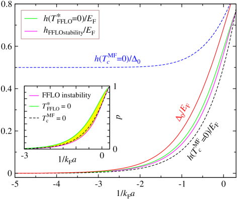
Figure 1: Gap $\Delta_{0}$ (red, as labeled) and $h$ along different lines, all in units of $E_{\text{F}}$, as well as their ratio $h(T_{\text{c}}^{\text{MF}}=0)/\Delta_{0}$ (blue dashed line), as a function of $1/k_{\text{F}}a$ for a 3D homogeneous Fermi gas. The calculation was done at the mean-field level without the particle-hole channel, which does not affect the ratio. Shown in the inset is the phase diagram of the stable FFLO phase. The upper boundary (green curve) is given by $T^{*}_{\text{FFLO}}=T_{\text{c}}^{\text{FFLO}}(\Delta=0)$, and the lower boundary (magenta curve) is given by the instability condition against phase separation. The Sarma $T_{\text{c}}^{\text{MF}}=0$ line (black dashed) lies within the FFLO phase. The $h$ value along these lines are shown in the main figure with the same color coding and line shapes.

It should be mentioned that the original Clogston derivation equates the free energy of the superfluid state at zero-field (i.e., $h=0$) with that of a polarized normal state at the threshold $h_{\text{c}}$, both at $T=0$. This approach is expected to be valid for the small $\Delta_{0}$ case in the perturbative sense. However, we argue that the balanced and the imbalanced cases are really distinct and cannot connect to each other continuously. This can be told from the fact that in the BCS regime, an arbitrarily small but nonzero population imbalance is sufficient to destroy superfluidity at precisely $T=0$ in the 3D homogeneous case (when stability is taken into account) Chien et al. (2006). For a finite $\Delta_{0}$, the “magnetic field” $h$ would have to jump from 0 of the balanced case to a value comparable to $\Delta_{0}$, implying that $h$ should not be treated perturbatively. Furthermore, there is no guarantee that the normal state in Clogston’s approach is a solution of the BCS gap equation in the zero gap limit. To check the CC limit, we calculate for a 3D homogeneous Fermi gas the gap $\Delta_{0}$ in the balanced case at zero $T$ and the field $h$ in the imbalanced case when the mean-field $T_{\text{c}}$ (also referred to as $T^{*}$) approaches 0, both as a function of pairing strength. The result is shown in Fig. 1, where we plot $\Delta_{0}$ for $h=0$ (red curve) and $h$ along the $T_{\text{c}}^{\text{MF}}=0$ curve (black dashed), as well as their ratio $h(T_{\text{c}}^{\text{MF}}=0)/\Delta_{0}$ (blue dashed), as a function of $1/k_{\text{F}}a$. This $h$ should be taken as $h_{\text{c}}$ since it is the boundary between a normal phase and polarized superfluid (also referred to as Sarma phase Sarma (1963)) with $q=0$ at $T=0$. The $T_{\text{c}}^{\text{MF}}=0$ curve for the Sarma phase in the $p$ – $1/k_{\text{F}}a$ plane can be easily obtained from the BCS-like mean-field $T_{\text{c}}$ equation with $\mathbf{q}=0$ and $T_{\text{c}}=0$, along with the fermion number constraints He et al. (2007). The figure indicates that the exact mean-field solution yields $h_{\text{c}}/\Delta_{0}=0.5$ in the BCS regime, substantially different from $1/\sqrt{2}$ given by CC, and this ratio increases to about 0.733 at unitarity. This result suggests that exact calculation is needed in order to obtain quantitatively accurate value for $h_{\text{c}}$. It corresponds to the $q=0$ limit of Eq. (8) and is not stable. The difference between this result and that of CC can likely be attributed to the possibility that the CC normal state does not satisfy the Thouless criterion while the present case does.

In the inset of Fig. 1, we show the stable FFLO phase at the mean-field level, as the yellow shaded region. The upper boundary (green curve) is given by the zero gap solution, $T^{*}_{\text{FFLO}}=0$, with a finite $q$ vector, which separates the FFLO phase from the normal Fermi gases. The lower phase boundary (magenta curve) is given by the instability condition of the FFLO phase against phase separation. Both boundary lines were taken from Ref. He et al. (2007). Next to but on the lower right side of this boundary are phase separated states. It is clear that the Sarma mean-field $T_{\text{c}}$ curve line (black dashed) lies completely within the stable FFLO phase, in agreement with the fact that the Sarma states along this curve are unstable against FFLO. We plot $h$ along these two boundaries (green and magenta solid curves) in the main figure. Interestingly, it turns out that, in the BCS limit, the ratio $h/\Delta_{0}$ along the lower boundary is close to $1/\sqrt{2}$, in agreement with Ref. Casalbuoni and Nardulli (2004). Meanwhile, the ratio along the upper boundary is close to 0.75. This leaves us with roughly the same FFLO window of $0.71<h/\Delta_{0}<0.75$ in the absence of the induced interactions.

Figure 2: The lowest-order diagram representing the induced interaction $U_{\text{ind}}(p_{1},p_{4})$. The solid and dashed lines represent fermion propagators and the interaction $g$ between fermions, respectively.

III Effects of the Induced Interaction on the FFLO window

The induced interaction was obtained originally by GMB in the BCS limit by the second-order perturbation Gor’kov and Melik-Barkhudarov (1961). For a scattering process with $p_{1}+p_{2}\rightarrow p_{3}+p_{4}$, the induced interaction for the diagram in Fig. 2 is expressed as

$$U_{\text{ind}}(p_{1},p_{4})=-g^{2}\chi_{\text{ph}}(p_{1}-p_{4}),$$ (10)

where $p_{i}=(\vec{k}_{i},\omega_{l_{i}})$ is a four vector. Including the induced interaction, the effective pairing interaction between atoms with different spins is given by

$$U_{\text{eff}}(p_{1},p_{4})\equiv U_{\text{eff}} = -g+U_{\text{ind}}(p_{1},p_{4})$$

$$= -g-g^{2}\chi_{\text{ph}}(p_{1}-p_{4}).$$

The polarization function $\chi_{\text{ph}}(p^{\prime})$ is given by

$$\chi_{\text{ph}}(p^{\prime}) = \sum_{p}\mathcal{G}_{0}^{b}(p)\mathcal{G}_{0}^{a}(p+p^{\prime})$$ (12)

$$= \int{{\rm{d}}^{3}k\over(2\pi)^{3}}\frac{f_{{\vec{k}}}^{b}-f_{{\vec{k}}+{\vec{q}}}^{a}}{i\Omega_{l}+\xi_{{\vec{k}},a}-\xi_{{\vec{k}}+{\vec{q}},b}},$$

where $f_{{\vec{k}}}^{\sigma}\equiv f(\xi_{\vec{k},\sigma})$, and $p^{\prime}=(\vec{q},\Omega_{l})$. This means that $U_{\text{eff}}$ is a function of momentum and frequency. The static polarization function is then,

$$\chi_{\text{ph}}(q,h) = -\frac{2m}{(2\pi)^{2}}\int\frac{\mathrm{d}k\,k^{2}}{2qk}\left[f_{k}^{\downarrow}\ln\left(\frac{q^{2}-4mh+2kq}{q^{2}-4mh-2kq}\right)+f_{k}^{\uparrow}\ln\left(\frac{q^{2}+4mh+2kq}{q^{2}+4mh-2kq}\right)\right],$$ (13)

where $q\equiv|\vec{q}|$. The above expression is usually computed in the zero temperature limit, with $f_{k}^{\downarrow,\uparrow}\to\Theta(k_{\text{F}}^{\downarrow,\uparrow}-k)$, where $\Theta(x)$ is the step function, such that the induced correction to the coupling $g$ is a (temperature independent) constant.

$$\chi_{\text{ph}}(q,h) \equiv \chi^{\downarrow}(q,h)+\chi^{\uparrow}(q,h)$$

$$= -\frac{m}{(2\pi)^{2}q}\int_{0}^{k_{\text{F}}^{\downarrow}}\mathrm{d}k\,k\ln\left(\frac{q^{2}-4mh+2kq}{q^{2}-4mh-2kq}\right){}-\frac{m}{(2\pi)^{2}q}\int_{0}^{k_{\text{F}}^{\uparrow}}\mathrm{d}k\,k\ln\left(\frac{q^{2}+4mh+2kq}{q^{2}+4mh-2kq}\right).$$

Equation (III) shows that the static polarization function in the case of a spin imbalanced Fermi gas separates into contributions from the spin-down and the spin-up like susceptibilities. The integration in $k$ gives

$$\chi_{\text{ph}}^{\downarrow}(q,h) = -\frac{m}{8\pi^{2}q}\left\{\left[{k_{\text{F}}^{\downarrow}}^{2}-\left(\frac{q^{2}-4mh}{2q}\right)^{2}\right]\ln\left|\frac{q^{2}-4mh+2qk_{\text{F}}^{\downarrow}}{q^{2}-4mh-2qk_{\text{F}}^{\downarrow}}\right|+k_{\text{F}}^{\downarrow}\left(\frac{q^{2}-4mh}{q}\right)\right\},$$ (15)

$$\chi_{\text{ph}}^{\uparrow}(q,h) = -\frac{m}{8\pi^{2}q}\left\{\left[{k_{\text{F}}^{\uparrow}}^{2}-\left(\frac{q^{2}+4mh}{2q}\right)^{2}\right]\ln\left|\frac{q^{2}+4mh+2qk_{\text{F}}^{\uparrow}}{q^{2}+4mh-2qk_{\text{F}}^{\uparrow}}\right|+k_{\text{F}}^{\uparrow}\left(\frac{q^{2}+4mh}{q}\right)\right\}.$$ (16)

The equations above can be put in a more convenient form, $\tilde{\chi}_{\text{ph}}^{\sigma}(x,y)\equiv\chi_{\text{ph}}^{\sigma}(q,h)$, where

$$\tilde{\chi}_{\text{ph}}^{\downarrow}(x,y) = -\frac{N(0)}{4}\left\{\sqrt{1-y}\left(1-\frac{y}{2x^{2}}\right)-\frac{1}{2x}\left[1-y-x^{2}\left(1-\frac{y}{2x^{2}}\right)^{2}\right]\ln\left|\frac{\sqrt{1-y}+\frac{y}{2x}-x}{\sqrt{1-y}-\frac{y}{2x}+x}\right|\right\}$$

$$= -N(0)L^{\downarrow}(x,y),$$

and

$$\tilde{\chi}_{\text{ph}}^{\uparrow}(x,y) = -\frac{N(0)}{4}\left\{\sqrt{1+y}\left(1+\frac{y}{2x^{2}}\right)-\frac{1}{2x}\left[1+y-x^{2}\left(1+\frac{y}{2x^{2}}\right)^{2}\right]\ln\left|\frac{\sqrt{1+y}-\frac{y}{2x}-x}{\sqrt{1+y}+\frac{y}{2x}+x}\right|\right\}$$

$$= -N(0)L^{\uparrow}(x,y),$$

where $x\equiv\frac{q}{2k_{\text{F}}}$, and $y\equiv\frac{h}{\mu}$. This allows us to write the polarization function of an imbalanced Fermi gas as

$$\tilde{\chi}_{\text{ph}}(x,y)=-N(0)L(x,y),$$ (19)

where $L(x,y)\equiv L^{\downarrow}(x,y)+L^{\uparrow}(x,y)$ is the generalized Lindhard function.

Notice that in the $y\to 0$ limit, $k_{\text{F}}^{\downarrow}=k_{\text{F}}^{\uparrow}=k_{\text{F}}$, such that $\tilde{\chi}_{\text{ph}}^{\downarrow}(x,0)=\tilde{\chi}_{\text{ph}}^{\uparrow}(x,0)\equiv\tilde{\chi}_{\text{ph}}(x)/2$ and we obtain the well-known (balanced) result

$$\tilde{\chi}_{\text{ph}}(x) = -\frac{m}{4\pi^{2}q}\left[k_{\text{F}}q-\left(k_{\text{F}}^{2}-\frac{q^{2}}{4}\right)\ln\left|\frac{q^{2}-2qk_{\text{F}}}{q^{2}+2qk_{\text{F}}}\right|\right]$$ (20)

$$= -N(0)L(x),$$

where $L(x)\equiv L(x,0)$ is the standard Lindhard function,

$$L(x)=\frac{1}{2}-\frac{1}{4x}(1-x^{2})\ln\left|\frac{1-x}{1+x}\right|.$$ (21)

In the scattering process the conservation of total momentum implies that $\vec{k}_{1}+\vec{k}_{2}=\vec{k}_{3}+\vec{k}_{4}$, with $\vec{k}_{1}=-\vec{k}_{2}$ and $\vec{k}_{3}=-\vec{k}_{4}$. The momentum $q$ is equal to the magnitude of $\vec{k}_{1}+\vec{k}_{3}$, so that $q=\sqrt{(\vec{k}_{1}+\vec{k}_{3}).(\vec{k}_{1}+\vec{k}_{3})}=\sqrt{\vec{k}_{1}^{2}+\vec{k}_{3}^{2}+2\vec{k}_{1}.\vec{k}_{3}}=\sqrt{\vec{k}_{1}^{2}+\vec{k}_{3}^{2}+2|\vec{k}_{1}||\vec{k}_{3}|\cos\phi}$, where $\phi$ is the angle between $\vec{k}_{1}$ and $\vec{k}_{3}$. Since both particles are at the Fermi surface, $|\vec{k}_{1}|=|\vec{k}_{3}|=k_{\text{F}}=\sqrt{2m\mu}$, thus, $q=k_{\text{F}}\sqrt{2(1+\cos\phi)}$, and consequently $x=\sqrt{2(1+\cos\phi)}/2$, which sets $0\leq x\leq 1$.

The s-wave part of the effective interaction is approximated by averaging the polarization function $\chi_{\text{ph}}(q)$ over the Fermi sphere, which means an average of the angle $\phi$ Heiselberg et al. (2000); Chen (2016); Petrov et al. (2003); Baranov et al. (2008); Yu et al. (2009); Kim et al. (2009); Yu and Yin (2010),

$$\langle\tilde{\chi}_{\text{ph}}(x,y)\rangle = \frac{1}{2}\int_{-1}^{1}\mathrm{d}\cos\phi~{}\tilde{\chi}_{\text{ph}}(x,y)$$ (22)

$$= -N(0)\left[\frac{1}{2}\int_{-1}^{1}\mathrm{d}\cos\phi~{}L(x,y)\right]$$

$$\equiv -N(0)\bar{L}(y),$$

where we have made use of Eq. (19). The quantity $\bar{L}$ characterizes the magnitude of GMB corrections in the presence of population imbalance. Shown in the inset of Fig. 4 is the behavior of $\bar{L}(y)$ as a function of imbalance $y$. In the $y\rightarrow 0$ limit, we have precisely $\bar{L}(0)=(1+2\ln 2)/3=0.795431454$, as given in Ref. Chen (2016) and other papers Yu and Yin (2010) for the balanced case. As $y$ increases from 0 to 1, $\bar{L}(y)$ decreases to 0.69, indicating that the particle-hole fluctuation effect becomes weaker due to the Fermi surface mismatch caused by population imbalance. This result is identical to that of Ref. Yu and Yin (2010).

Taking into account the GMB correction, the divergence of the $T$ matrix in Eq. (7) is now given by

$$t^{-1}(\mathbf{q},0)=\left(-\frac{1}{g}+\langle\tilde{\chi}_{\text{ph}}(x,y)\rangle\right)+\chi({\vec{q}},0)=0,$$ (23)

which can be obtained by replacing $g$ in Eq. (7) with $U_{\text{eff}}$, as given in Eq. (III). This expression has been shown to be correct when the more complicate $T$ matrix in the particle-hole channel is included self-consistently Chen (2016). This yields a GMB corrected solution $\Delta_{0}^{\text{GMB}}$ satisfying $\dfrac{h(y)}{\Delta_{0}^{\text{GMB}}}=\left(\dfrac{h(y)}{\Delta_{0}}\right)^{\text{MF}}$ and $\Delta^{\text{GMB}}(y)=\Delta(y)e^{-\bar{L}(y)}$, with $\Delta_{0}\equiv\Delta(y=0,T=0)$ and $\Delta_{0}^{\text{GMB}}=\Delta^{\text{GMB}}(y=0,T=0)$. This amounts to

$$\frac{h_{\text{s}}}{\Delta_{0}}=\left(\frac{h_{\text{s}}}{\Delta_{0}}\right)^{\text{MF}}e^{-\bar{L}(y_{\text{s}})},$$ (24)

where $y_{\text{s}}=h_{\text{s}}/\mu$, and $\left(\frac{h_{\text{s}}}{\Delta_{0}}\right)^{\text{MF}}\simeq 0.75$ is the MF result without the GMB corrections.

It is well known that the zero temperature BCS pairing gap (at $y=0$) is modified due to the particle-hole channel effect (or GMB correction) as Heiselberg et al. (2000); Chen (2016)

$$\Delta_{0}^{\text{GMB}} = \frac{\Delta_{0}}{(4e)^{1/3}}=\frac{8}{e^{2}}\frac{1}{(4e)^{1/3}}\mu e^{-\pi/2k_{\text{F}}|a|}$$ (25)

$$= \left(\frac{2}{e}\right)^{7/3}\mu e^{-\pi/2k_{\text{F}}|a|}.$$

Note here that in the expression for $\Delta_{0}$, the chemical potential $\mu$ plays the role of $E_{\text{F}}$. This can be readily obtained following the standard derivation in the BCS framework, but allowing the Fermi level to evolve continuously as one does for the BCS-BEC crossover Leggett (1980). This automatically corrects the moving density of states as the Fermi level changes, even though the approximation becomes less accurate by replacing the full momentum space integral by an energy integral with the density of states fixed at the Fermi level. Shown in Fig. 3 is a comparison between the calculated $\Delta_{0}$ and different analytical approximations. The blue dot-dashed line is the expression in the weak coupling limit, with $\mu$ pinned at $E_{F}$. Our corrected expression is shown as the red solid curve. Both are to be compared with $\Delta_{0}$ (green solid curve), which is calculated self-consistently in the context of BCS-BEC crossover. It is evident that our corrected expression is quantitatively good all the way from the BCS through the unitary limit.

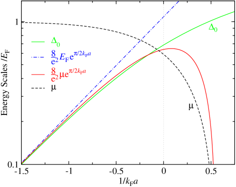
Figure 3: Behavior of self-consistently calculated zero temperature $\mu$ (black dashed) and $\Delta_{0}$ (green solid), as well as the weak coupling BCS expression (blue dot-dashed) and our corrected approximation (red solid line) for $\Delta_{0}$, in units of $E_{F}$, as a function of $1/k_{F}a$ for a 3D homogeneous Fermi gas.

In order to find the appropriate $y$ for consistently evaluating Eq. (24), we take the expression for the GMB gap at unitarity, $1/k_{\text{F}}a=0$, and obtain

$$\Delta_{0}^{\text{GMB}}=\left(\frac{2}{e}\right)^{7/3}\!\!\!\mu\simeq 0.49\mu$$ (26)

for $y=0$. Note that this is very close to the more complete solution of $\Delta_{0}^{\text{GMB}}=0.42E_{\text{F}}=0.50\mu$ with $\mu=0.837E_{\text{F}}$, calculated with the full particle-hole $T$ matrix included at the $G_{0}G_{0}$ level Chen (2016). According to Eq. (25), when taking into account the GMB correction, the original $h_{\text{c}}/\Delta_{0}=1/\sqrt{2}$ is transformed to $h_{\text{c}}^{\text{GMB}}/\Delta_{0}^{\text{GMB}}=1/\sqrt{2}$, which, with Eq. (26), yields $h_{\text{c}}^{\text{GMB}}/\mu\equiv y_{\text{c}}=\left(\frac{2}{e}\right)^{7/3}\frac{1}{\sqrt{2}}=0.3455$ at unitarity.

In Eq. (24), we approximate $y_{\text{s}}\equiv h_{\text{s}}/\mu$ by $y_{\text{c}}$ in $\bar{L}(y_{\text{s}})$, and obtain $\bar{L}=0.7857$, and thus

$$\frac{h_{\text{s}}^{\text{GMB}}}{\Delta_{0}}=0.4558\left(\frac{h_{\text{s}}}{\Delta_{0}}\right)^{\text{MF}}\simeq 0.342.$$ (27)

Alternatively, one can take $\dfrac{h_{\text{s}}^{\text{GMB}}}{\Delta_{0}^{\text{GMB}}}=\left(\dfrac{h_{\text{s}}}{\Delta_{0}}\right)^{\text{MF}}$ and obtain immediately

$$\frac{h_{\text{s}}^{\text{GMB}}}{\Delta_{0}}=\frac{1}{(4e)^{1/3}}0.75=0.339,$$ (28)

which agrees with Eq. (27). On the other hand, with the shifted interaction strength, the CC limit is modified to

$$\frac{h_{\text{c}}^{\text{GMB}}}{\Delta_{0}} = \frac{1}{(4e)^{1/3}}\frac{1}{\sqrt{2}}=0.319.$$ (29)

Combining Eq. (27) and Eq. (29), we conclude that the screening of the medium (i.e., the induced interactions) has shrunk the FFLO window to

$$0.32\lesssim h/\Delta_{0}\lesssim 0.34\,.$$ (30)

IV Effects of induced interactions in the presence of impurities

The above calculations in Section III have been done assuming the system is clean. However, this is not always true, especially for a superconductor, for which impurities and dislocations are easy to find. Impurities may cause a finite lifetime for the quasiparticles. In quasi-one-dimensional organic superconductors, for instance, the issue of lifetime effects arise from nonmagnetic impurities or defects Ardavan et al. (2012). These impurities may add to the complexity of the effect of particle-hole fluctuations, and thus deserve careful inspection.

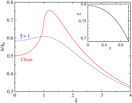
Figure 4: The ratio $h/\Delta_{0}$ as a function of $q$. The solid curve is for $\gamma=0$, and attains its maximum value $\simeq 0.75$, at $\bar{q}=\bar{q}_{\text{c}}\simeq 1.2$. The dashed curve is for $\tilde{\gamma}=1$ and shows a significant reduction of the maximum value of $h/\Delta_{0}$. Shown in the inset is the behavior of $\bar{L}$ as a function of $y=h/\mu$.

In this section we show that, indeed, the FFLO window may be strongly affected by impurity effects Agterberg and Yang (2001). We shall only consider nonmagnetic weak impurities in the Born limit Che et al. (2017), which mainly lead to a spectral broadening $\gamma$ for the fermions . Then we rederive everything in the presence of the spectral broadening. For the nonmagnetic impurities which we consider, possible modification to the real part of quasiparticle dispersion may be absorbed into the chemical potential. Along with the simplification of the imaginary part by a constant parameter $\gamma$, these nonmagnetic impurities satisfy the Anderson’s theorem in the BCS regime Anderson (1959). As the gap becomes large, the small gap approximation assumed by Anderson’s theorem is no longer valid. However, a large $s$-wave gap itself is very robust against weak impurities Che et al. (2017). In Fig. 4, we show the numerical solutions of $h/\Delta_{0}$ as a function of $\bar{q}$ from Eqs. (8) and (32), for both the clean limit i.e., $\gamma=0$ (red curve), and the dirty case with $\tilde{\gamma}\equiv\gamma/2h=1$ (blue dashed line), where $\gamma=\tau^{-1}$ is the inverse of the lifetime of a quasiparticle in the normal phase. The clean case has a maximum value at $\bar{q}=\bar{q}_{\text{c}}\simeq 1.2$, which gives $h/\Delta_{0}=h_{\text{s}}/\Delta_{0}\simeq 0.75$, as obtained by the analytical calculations in Section II. In the dirty case, the maximum has shifted toward lower $\bar{q}$, and the maximum ratio $h_{\text{s}}/\Delta_{0}$ has decreased significantly. This inevitably narrows the FFLO window. When this ratio drops below $1/\sqrt{2}$, the FFLO window will be gone and thus the FFLO phase will disappear at the mean-field level.

Impurities in principle have an effect on the GMB correction, mainly via changing the chemical potential $\mu$. However, we point out this is only a minor secondary effect, since the change in $\mu$ due to impurities is often very small, especially for Born impurities, which cannot induce an impurity band outside the Fermi sphere Chen and Schrieffer (2002). The GMB correction used in the present calculation has been done at the lowest level approximation Chen (2016), without considering the gap effect at the Fermi level. Therefore, we believe that at this level, one can safely neglect the impurity effect on the GMB correction to the pairing strength. Therefore, we conclude that the effect of particle-hole fluctuations may be largely taken care of by assuming that it is encoded in an effective pairing strength, a la Eq. (23). One only needs to roughly rescale $h_{s}$ obtained in the presence of impurities by same factors $(4e)^{-1/3}$ as in the clean case. Hence, it does not have to appear explicitly in our impurity derivations below. It should be noted, however, that $h_{\text{c}}$ is unaffected by impurities, for two reasons. As given by the Anderson’s theorem, $\Delta_{0}$ is unaffected by the weak nonmagnetic impurities. The thermodynamics calculation of $h_{\text{c}}$, which involves the free energy density of magnetic field, $H_{0}^{2}/8\pi$, as given by Clogston Clogston (1962), is insensitive to impurities. Therefore, $h_{\text{c}}$ is only subject to the GMB correction.

Considering the finite lifetime of the quasi-particle states in the momentum representation, the pair susceptibility $\chi$ is found, via Eqs. (5) and (23), by the standard method of including a finite imaginary part to the Green’s function Leung (1975); Abrikosov et al. (1963), $\mathcal{G}_{0}^{\sigma}(K)=1/(i\omega_{l}-\xi_{\vec{k}\sigma}+i\gamma\,\mathrm{sgn}(\xi_{\vec{k}\sigma}))$. After somewhat lengthy but straightforward derivations (as shown in Appendix A), the real part of the particle-particle dynamic pair susceptibility can be written as,

$$\mathrm{Re}\bar{\chi}({\bar{q}}) = N(0)\left[1+\ln\left(\frac{2\omega_{\text{c}}}{2h}\right)+\frac{1}{4\bar{q}}\left(1-{\bar{q}}\right)\ln\left((1-{\bar{q}})^{2}+\tilde{\gamma}^{2}\right)-\frac{1}{4\bar{q}}\left(1+{\bar{q}}\right)\ln\left((1+{\bar{q}})^{2}+\tilde{\gamma}^{2}\right)\right],$$ (31)

which is the counterpart of Eq. (6). This approach is formally close to that used to investigate the effect of non-magnetic impurities in one dimensional imbalanced Fermi gases Caldas and Continentino (2013), and in two Houzet and Mineev (2006) and three Takada (1970) dimensional FFLO superconductors.

With $\text{Re}\bar{\chi}({\bar{q}})$ from Eq. (31) the divergence of the $T$ matrix now yields

$$\frac{h}{\Delta_{0}}=\frac{e}{2}\left[(1-\bar{q})^{2}+\tilde{\gamma}^{2}\right]^{{\frac{1-\bar{q}}{4\bar{q}}}}\left[(1+\bar{q})^{2}+\tilde{\gamma}^{2}\right]^{-{\frac{1+\bar{q}}{4\bar{q}}}}.\hskip 28.45274pt$$ (32)

Notice that in the limit $\tilde{\gamma}\to 0$ in Eqs. (31) and (32), the standard results in Eqs. (6) and (8) are recovered.

Instead of being a solution of Eq. (9), the critical reduced momentum $\bar{q}_{\text{c}}$ is now given by the solution of

$$2\bar{q}_{\text{c}}\left[\frac{(1+\bar{q}_{\text{c}})^{2}}{(1+\bar{q}_{\text{c}})^{2}+\tilde{\gamma}^{2}}\right. + \left.\frac{(1-\bar{q}_{\text{c}})^{2}}{(1-\bar{q}_{\text{c}})^{2}+\tilde{\gamma}^{2}}\right]$$

$$=\ln\left[\frac{(1+\bar{q}_{\text{c}})^{2}+\tilde{\gamma}^{2}}{(1-\bar{q}_{\text{c}})^{2}+\tilde{\gamma}^{2}}\right].$$

For $\tilde{\gamma}=1$, for instance, the numerical solution of the equation above yields $\bar{q}_{\text{c}}\simeq 1.01$, besides the trivial solution $\bar{q}_{\text{c}}=0$. This leads to $h_{\text{s}}\simeq 0.61\Delta_{0}$ for the location of the FFLO transition, (which transforms to $h_{\text{s}}^{\text{GMB}}\approx 0.28\Delta_{0}$), in agreement with Fig. 4. However, this value is beyond the critical value $\tilde{\gamma}_{\text{c}}=0.3$, which gives $h_{\text{s}}^{\text{critical}}/\Delta_{0}\simeq 0.71=h_{\text{c}}/\Delta_{0}$, or $h_{\text{s}}^{\text{GMB,critical}}=0.32\Delta_{0}=h_{\text{c}}^{\text{GMB}}$, for closing the FFLO window. This means that at this critical value of $\gamma$ the system undergoes a first-order quantum phase transition from the BCS to the polarized normal phase. Conversely, with infinite life time ($\gamma=0$) the FFLO window remains open with the “unperturbed” limits $h_{\text{c}}^{\text{GMB}}<h<h_{\text{s}}^{\text{GMB}}$, as given by Eq. (30). This nontrivial result comes from the fact that $h_{\text{c}}$ and $h_{\text{s}}$ respond to impurities differently.

V Further Discussions

It should be noted that we have in fact considered only the FF case. This is justified in that there is no self-consistent way to calculate the LO and higher order crystalline LOFF phases when the pairing gap is large. In the original LO paper Larkin and Ovchinnikov (1965), the LO state order parameter is treated as a small perturbation to the noninteracting fermion propagator so that in the evaluation of all the diagrams, the Green’s function is treated at the noninteracting level. Such a perturbative treatment necessarily breaks down in the unitary regime, where the gap is large, comparable to the Fermi energy. In addition, in the presence of two wavevectors $\pm\mathbf{q}$, a simple diagrammatic analysis shows that it will generate an infinite series of components of wavevector $\pm n\mathbf{q}$ ($n=0,1,2,...$) in the order parameter Datta et al. (2019). Indeed, many later works on LO and higher order crystalline states treat the order parameters as an expansion parameter, in a Ginzburg-Landau type of formalism Buzdin and Kachkachi (1997); Agterberg and Yang (2001); Adachi and Ikeda (2003); Vorontsov et al. (2008), and thus they are appropriate only in the weak pairing regime. Therefore, unlike the FF case, there is no simple field-theoretical approach to the LO and higher order crystalline phases beyond the perturbative mean-field treatment with a truncation of the series of the wavevectors Chen et al. (2007). This makes it more difficult to include the GMB or particle-hole fluctuation effect using field-theoretical techniques Yu et al. (2009); Yu and Yin (2010); Chen (2016). It remains a challenging issue for the future to treat self-consistently the effect of particle-hole fluctuations on the LO and higher order crystalline FFLO states beyond the mean-field level.

In the presence of inhomogeneity, the Bogoliubov – de Gennes (BdG) treatment is often used Cui and Yang (2008). It is particularly useful for treating Fermi gases in a trap. However, it should be emphasized that BdG is also a mean-field treatment, albeit in real space. In the presence of multiple wavevectors, the complexity of the generalized formalism increases rapidly (see, e.g., Datta et al. (2019)). There has been thus far no report in the literature of incorporating particle-hole fluctuations in the BdG formalism.

It should be pointed out that, for population imbalanced Fermi gases in a trap, the local population imbalance $p$ varies as a function of the radius. While an inverted density distribution is possible Liao et al. (2010); Wang et al. (2013), in most cases, $p$ increases from zero (or nearly zero depending on the temperature) at the trap center to unity at the trap edge. One may think of the radius as an equivalent of the imbalance $p$ in the inset of Fig. 1. At low $T$, except for the BEC regime, one may find that the FFLO solution exists at certain radius, or inside a narrow shell near this radius, under the local density approximation (LDA). The thickness of the shell, relative to the coherence length, may have a strong influence as to whether a FFLO solution exists. In such a case, BdG may have an advantage over LDA.

Our impurity treatment has been restricted to nonmagnetic impurities in the Born limit, following the approach of Anderson Anderson (1959) and Abrikosov and Gor’kov Abrikosov and Gor’kov (1959); Abrikosov et al. (1963). This assumes randomly distributed weak impurities, whose effect can mainly be simplified as a finite life time effect in the quasiparticles. Recent works Han and Sa de Melo (2011); Che et al. (2017) show that weak disorders do not significantly affect $T_{c}$ of an $s$-wave BCS superfluid in accordance with Anderson’s theorem Anderson (1959), and the superfluid is more robust to the presence of disorder in the unitary regime. There has been treatment beyond the Born limit, in the context of $d$-wave high $T_{c}$ superconductors Hirschfeld et al. (1988); Chen and Schrieffer (2002); Balatsky et al. (2006) and $s$-wave atomic Fermi gases in the BCS-BEC crossover Palestini and Strinati (2013); Che et al. (2017). There are of course also treatments of pair breaking, magnetic disorders or impurities in superconductors Fowler and Maki (1970); Maki (1972); Bickers and Zwicknagl (1987); Vernier et al. (2011); Riegger et al. (2018). It would be interesting to investigate how an FFLO phase responds to magnetic impurities. Apparently, the impurity averaging technique has been widely applied to the impurity treatment for the FFLO states as well Aslamazov (1959); Takada (1970); Agterberg and Yang (2001); Adachi and Ikeda (2003); Vorontsov et al. (2008).

Beside treating random impurities in an averaged fashion, some studies treat impurities locally Wang et al. (2007); Cui and Yang (2008); Yanase (2009); Datta et al. (2019), especially in the case of single, few, or non-uniformly distributed impurities. Such impurities, if strong enough, may lead to localized states Vernier et al. (2011). When averaged over a large number of uniform random distributions, it is expected that, for weak impurities, these two approaches yield compatible results. Indeed, our result is in agreement with the BdG based findings of Ref. Cui and Yang (2008) for $s$-wave pairing, in that the FFLO state is much more sensitive to disorders than the BCS state, and that it can survive moderate disorder strength but may be fully suppressed by higher impurity levels. Both results indicate that a low impurity level, or equivalently a long mean free path, is needed for the FFLO state to survive the disorder effect.

It should be noted that, BdG calculations are usually done in a discretized lattice, which necessarily needs to be much larger than the coherence length $\xi_{0}$ of the superfluid, of the order of $\hbar v_{\textbf{F}}/\Delta$. In the BCS regime, the gap is small so that $\xi_{0}$ is huge. For a $d$-wave superconductor, due to the nonlocal effect Kosztin and Leggett (1997), $\xi_{0}$ diverges in the nodal directions. Both these cases raise a concern about the quantitative reliability for BdG calculations, when the lattice size is not big enough.

While we consider the ground state only, the treatment in principle can be extended to finite temperatures at the mean-field level. Without considering the FFLO state, the GMB effect acts essentially as a reduction of the pairing interaction strength (with a small temperature dependence) Chen (2016). This would thus lead to a reduction to both $T_{\text{c}}$ and $\Delta_{0}$, with a slight difference between finite and zero $T$. (This difference vanishes in the BCS limit). In this case, there should be a GMB-reduced pairing temperature, $T^{*,\text{GMB}}$, at which pairs form but do not Bose condense. Then, at a lower temperature, $T_{\text{c}}^{\text{GMB}}$, phase coherence sets in and pairs start to Bose condense. The situation is different with a nonzero FFLO wavevector $\mathbf{q}$, which is pertinent to a high population imbalance or a high magnetic field. While the FFLO mean-field solution usually exists at low $T$, when pairing fluctuations, which usually lead to the formation of a pseudogap, are taken into account, the mean-field FFLO states become unstable, in the absence of extrinsic symmetry breaking factors such as spatial anisotropy and lattices, as found in Ref. Wang et al. (2018). Similar results were found by others as well Samokhin and Mar’enko (2006b); Radzihovsky and Vishwanath (2009); Radzihovsky (2011). Even at the mean-field level, there may exist an intermediate temperature pseudogap regime, between $T^{*,\text{GMB}}$ and $T_{\text{c}}^{\text{MF,GMB}}$. An example of such a pseudogap regime, calculated in the absence of the GMB corrections, can be found in Ref. Chen (2016).

Finally, it is known that in the $H$–$T$ phase diagram of a superconductor, the existence of the mean-field FFLO phase extends the $H_{\text{c,2}}$ line at low $T$ towards the high field side of its BCS counterpart, leading to a kink-like feature at the tricritical point which signals the onset of the FFLO state. Since the field strength $H$ is proportionally related to the population imbalance $p$, a counterpart $T$–$p$ phase diagram can often be found in the atomic Fermi gas literature, e.g., Refs. He et al. (2006); Wang et al. (2017). Now that the GMB effect leads mainly to a reduction of the pairing interaction strength, it is expected that the $T$–$p$ phase diagram looks qualitatively similar to its clean counterpart at the reduced pairing strength.

VI Conclusion

In summary, we have investigated in homogeneous 3D systems the GMB correction to the chemical potential difference $h/\Delta_{0}$, which is responsible for the transition to the FFLO phase. We find at the mean-field level that the window for the FFLO phase to exist has been reduced by a factor of $(4e)^{-1/3}$. Therefore, the region in the phase space that otherwise possesses an FFLO order will take alternative solutions, such as phase separation and polaronic normal state. This shall thus further confine the phase space where the true stable solution is yet to be determined.

We have also considered the GMB effect on the FFLO window in the presence of weak (nonmagnetic) impurities or defects, in terms of a finite lifetime $\tau=1/\gamma$ of the quasi-particle excitations. We find that a high impurity level leads to a reduction in the critical field $h_{\text{s}}$ of the continuous phase transition between the FFLO and the normal phase. This will shrink or completely destroy the FFLO window.

Appendix A Calculation of the pair susceptibility $\chi$ in the presence of impurities

The dynamic pair susceptibility is given by,

$$\chi({\vec{q}},\Omega) = \sum_{\vec{k}}\frac{1-f(\xi_{\vec{k}-\vec{q}/2,\uparrow})-f(\xi_{\vec{k}+\vec{q}/2,\downarrow})}{\xi_{\vec{k}-\vec{q}/2,\uparrow}+\xi_{\vec{k}+\vec{q}/2,\downarrow}-\Omega}$$

$$= \frac{1}{2}\sum_{\vec{k}}\frac{\tanh(\beta\xi_{\vec{k}-\vec{q}/2,\uparrow})+\tanh(\beta\xi_{\vec{k}+\vec{q}/2,\downarrow})}{\xi_{\vec{k}-\vec{q}/2,\uparrow}+\xi_{\vec{k}+\vec{q}/2,\downarrow}-\Omega}\,,$$

which can be rewritten as

$$\chi({\vec{q}},\Omega)=\frac{1}{2}\sum_{\vec{k}}\left[\frac{\tanh(\beta\xi_{\vec{k},\uparrow})}{\xi_{\vec{k},\uparrow}+\xi_{\vec{k}+\vec{q},\downarrow}-\Omega}+\frac{\tanh(\beta\xi_{\vec{k},\downarrow})}{\xi_{\vec{k}-\vec{q},\uparrow}+\xi_{\vec{k},\downarrow}-\Omega}\right]\,.$$ (35)

The denominators can be approximated as $\xi_{\vec{k},\uparrow}+\xi_{\vec{k}+\vec{q},\downarrow}-\Omega\simeq 2(\xi_{\vec{k},\uparrow}+h+a\cos\theta-\Omega/2)$ and $\xi_{\vec{k}-\vec{q},\uparrow}+\xi_{\vec{k},\downarrow}-\Omega\simeq 2(\xi_{\vec{k},\downarrow}-h-a\cos\theta-\Omega/2)$, where $a\equiv kq/2m$, and and $\theta$ is the angle between $\vec{k}$ and $\vec{q}$. Terms of order $q^{2}$ and higher have been neglected. Then we obtain

$$\chi({\vec{q}},\Omega) = \frac{1}{4}\sum_{\vec{k}}\Bigg{[}\frac{\tanh(\beta\xi_{\vec{k},\uparrow})}{\xi_{\vec{k},\uparrow}+h+a\cos\theta-\Omega/2}$$ (36)

$${}+\frac{\tanh(\beta\xi_{\vec{k},\downarrow})}{\xi_{\vec{k},\downarrow}-h-a\cos\theta-\Omega/2}\Bigg{]}.$$

Now we first integrate out $\theta$ over a narrow momentum shell with an energy cutoff $\omega_{c}$ near the Fermi level, followed by analytical continuation, $\Omega\to\Omega+i\gamma$. Then we arrive in the static limit at

$$\mathrm{Re} \chi({\vec{q}},\gamma)$$

$${}=\frac{m^{2}}{4\pi^{2}q}\int_{0}^{\omega_{c}}\!\!\!\!\mathrm{d}\omega\;\tanh\left(\!\frac{\beta\omega}{2}\right)\,\ln\frac{(\omega+h+a)^{2}+\gamma^{2}/4}{(\omega+h-a)^{2}+\gamma^{2}/4},$$

where $a\to v_{\text{F}}q/2$, and $v_{\text{F}}=k_{\text{F}}/m$ is the Fermi velocity. Taking now the zero temperature limit, and integrating over $\omega$ we obtain Eq. (31).

References

- Bardeen et al. (1957) J. Bardeen, L. N. Cooper, and J. R. Schrieffer, Theory of superconductivity, Phys. Rev. 108, 1175 (1957).
- Chen et al. (2007) Q. J. Chen, Y. He, C.-C. Chien, and K. Levin, Theory of superfluids with population imbalance: Finite-temperature and BCS-BEC crossover effects, Phys. Rev. B 75, 014521 (2007).
- Giorgini et al. (2008) S. Giorgini, L. P. Pitaevskii, and S. Stringari, Theory of ultracold atomic Fermi gases, Rev. Mod. Phys. 80, 1215 (2008).
- Inguscio et al. (2007) M. Inguscio, W. Ketterle, and C. Salomon, eds., Proceedings of the International School of Physics ”Enrico Fermi” Course CLXIV (IOS Press, Amsterdam, 2007).
- Bloch et al. (2008) I. Bloch, J. Dalibard, and W. Zwerger, Many-body physics with ultracold gases, Rev. Mod. Phys. 80, 885 (2008).
- Fulde and Ferrell (1964) P. Fulde and R. A. Ferrell, Superconductivity in a strong spin-exchange field, Phys. Rev. 135, A550 (1964).
- Larkin and Ovchinnikov (1965) A. I. Larkin and Y. N. Ovchinnikov, Inhomogeneous state of superconductors, Sov. Phys. JETP 20, 762 (1965), [Zh. Eksp. Teor. Fiz. 47, 1136 (1964)].
- Shimahara (1999) H. Shimahara, Stability of Fulde-Ferrell-Larkin-Ovchinnikov state in type-II superconductors against the phase fluctuations, Physica B 259-261, 492 (1999).
- Shimahara (1998) H. Shimahara, Structure of the Fulde-Ferrell-Larkin-Ovchinnikov state in two-dimensional superconductors, J. Phys. Soc. Jpn. 67, 736 (1998).
- Samokhin and Mar’enko (2006a) K. V. Samokhin and M. S. Mar’enko, Quantum fluctuations in Larkin-Ovchinnikov-Fulde-Ferrell superconductors, Phys. Rev. B 73, 144502 (2006a).
- Kinnunen et al. (2018) J. J. Kinnunen, J. E. Baarsma, J.-P. Martikainen, and P. Törmä, The Fulde–Ferrell–Larkin–Ovchinnikov state for ultracold fermions in lattice and harmonic potentials: a review, Reports on Progress in Physics 81, 046401 (2018).
- Koponen et al. (2008) T. K. Koponen, T. Paananen, J.-P. Martikainen, M. R. Bakhtiari, and P. Törmä, FFLO state in 1-, 2- and 3-dimensional optical lattices combined with a non-uniform background potential, New Journal of Physics 10, 045014 (2008).
- Ptok (2017) A. Ptok, The influence of the dimensionality of the system on the realization of unconventional Fulde–Ferrell–Larkin–Ovchinnikov pairing in ultra-cold Fermi gases, Journal of Physics: Condensed Matter 29, 475901 (2017).
- Revelle et al. (2016) M. C. Revelle, J. A. Fry, B. A. Olsen, and R. G. Hulet, 1D to 3D crossover of a spin-imbalanced Fermi gas, Phys. Rev. Lett. 117, 235301 (2016).
- Wang et al. (2018) J. B. Wang, Y. M. Che, L. F. Zhang, and Q. J. Chen, Instability of Fulde-Ferrell-Larkin-Ovchinnikov states in atomic Fermi gases in three and two dimensions, Phys. Rev. B 97, 134513 (2018), and references therein.
- Schirotzek et al. (2009) A. Schirotzek, C.-H. Wu, A. Sommer, and M. W. Zwierlein, Observation of Fermi polarons in a tunable Fermi liquid of ultracold atoms, Phys. Rev. Lett. 102, 230402 (2009).
- Nascimbène et al. (2009) S. Nascimbène, N. Navon, K. J. Jiang, L. Tarruell, M. Teichmann, J. McKeever, F. Chevy, and C. Salomon, Collective oscillations of an imbalanced Fermi gas: Axial compression modes and polaron effective mass, Phys. Rev. Lett. 103, 170402 (2009).
- Shin et al. (2006) Y. Shin, M. W. Zwierlein, C. H. Schunck, A. Schirotzek, and W. Ketterle, Observation of phase separation in a strongly interacting imbalanced Fermi gas, Phys. Rev. Lett. 97, 030401 (2006).
- Partridge et al. (2006) G. B. Partridge, W. Li, R. I. Kamar, Y. A. Liao, and R. G. Hulet, Pairing and phase separation in a polarized Fermi gas, Science 311, 503 (2006).
- Clogston (1962) A. M. Clogston, Upper limit for the critical field in hard superconductors, Phys. Rev. Lett. 9, 266 (1962).
- Chandrasekhar (1962) B. S. Chandrasekhar, A note on the maximum critical field of high-field superconductors, Appl. Phys. Lett. 1, 7 (1962).
- Chien et al. (2006) C. C. Chien, Q. J. Chen, Y. He, and K. Levin, Intermediate temperature superfluidity in a Fermi gas with population imbalance, Phys. Rev. Lett. 97, 090402 (2006).
- Pao et al. (2006) C.-H. Pao, S.-T. Wu, and S.-K. Yip, Superfluid stability in the BEC-BCS crossover, Phys. Rev. B 73, 132506 (2006).
- Chen et al. (2006) Q. J. Chen, Y. He, C.-C. Chien, and K. Levin, Stability conditions and phase diagrams for two-component Fermi gases with population imbalance, Phys. Rev. A 74, 063603 (2006).
- Sheehy and Radzihovsky (2006) D. E. Sheehy and L. Radzihovsky, BEC-BCS crossover in “magnetized” Feshbach-resonantly paired superfluids, Phys. Rev. Lett. 96, 060401 (2006).
- Bedaque et al. (2003) P. F. Bedaque, H. Caldas, and G. Rupak, Phase separation in asymmetrical fermion superfluids, Phys. Rev. Lett. 91, 247002 (2003).
- Caldas (2004) H. Caldas, Cold asymmetrical fermion superfluids, Phys. Rev. A 69, 063602 (2004).
- Radzihovsky and Sheehy (2010) L. Radzihovsky and D. E. Sheehy, Imbalanced Feshbach-resonant Fermi gases, Rep. Prog. Phys. 73, 076501 (2010).
- Chevy and Mora (2010) F. Chevy and C. Mora, Ultra-cold polarized Fermi gases, Rep. Prog. Phys. 73, 112401 (2010).
- Zwerger (2012) W. Zwerger, ed., The BCS-BEC Crossover and the Unitary Fermi Gas, Lecture Notes in Physics, Vol. 836 (Springer Berlin Heidelberg, Berlin, Heidelberg, 2012).
- Zwierlein et al. (2006) M. W. Zwierlein, C. H. Schunck, A. Schirotzek, and W. Ketterle, Direct observation of the superfluid phase transition in ultracold Fermi gases, Nature (London) 442, 54 (2006).
- Nascimbène et al. (2010) S. Nascimbène, N. Navon, K. J. Jiang, F. Chevy, and C. Salomon, Exploring the thermodynamics of a universal Fermi gas, Nature 463, 1057 (2010).
- Navon et al. (2010) N. Navon, S. Nascimbene, F. Chevy, and C. Salomon, The equation of state of a low-temperature Fermi gas with tunable interactions, Science 328, 729 (2010).
- Nascimbène et al. (2011) S. Nascimbène, N. Navon, S. Pilati, F. Chevy, S. Giorgini, A. Georges, and C. Salomon, Fermi-liquid behavior of the normal phase of a strongly interacting gas of cold atoms, Phys. Rev. Lett. 106, 215303 (2011).
- Lewenstein et al. (2007) M. Lewenstein, A. Sanpera, V. Ahufinger, B. Damski, A. Sen(De), and U. Sen, Ultracold atomic gases in optical lattices: mimicking condensed matter physics and beyond, Adv. Phys. 56, 243 (2007).
- Osterloh et al. (2002) A. Osterloh, L. Amico, G. Falci, and R. Fazio, Scaling of entanglement close to a quantum phase transition, Nature 416, 608–610 (2002).
- Bianchi et al. (2003) A. Bianchi, R. Movshovich, C. Capan, P. G. Pagliuso, and J. L. Sarrao, Fulde-Ferrell-Larkin-Ovchinnikov Superconducting State in CeCoIn5, Phys. Rev. Lett. 91, 187004 (2003).
- Radovan et al. (2003) H. A. Radovan, N. A. Fortune, T. P. Murphy, S. T. Hannahs, E. C. Palm, S. W. Tozer, and D. Hall, Magnetic enhancement of superconductivity from electron spin domains, Nature 425, 51 (2003).
- Kenzelmann et al. (2008) M. Kenzelmann, T. Straessle, C. Niedermayer, M. Sigrist, B. Padmanabhan, M. Zolliker, A. D. Bianchi, R. Movshovich, E. D. Bauer, J. L. Sarrao, and J. D. Thompson, Coupled superconducting and magnetic order in CeCoIn5, Science 321, 1652 (2008).
- Kumagai et al. (2006) K. Kumagai, M. Saitoh, T. Oyaizu, Y. Furukawa, S. Takashima, M. Nohara, H. Takagi, and Y. Matsuda, Fulde-Ferrell-Larkin-Ovchinnikov state in a perpendicular field of quasi two-dimensional CeCoIn5, Phys. Rev. Lett. 97, 227002 (2006).
- Koutroulakis et al. (2010) G. Koutroulakis, M. D. Stewart, V. F. Mitrović, M. Horvatić, C. Berthier, G. Lapertot, and J. Flouquet, Field evolution of coexisting superconducting and magnetic orders in CeCoIn5, Phys. Rev. Lett. 104, 087001 (2010).
- Tokiwa et al. (2012) Y. Tokiwa, E. D. Bauer, and P. Gegenwart, Quasiparticle entropy in the high-field superconducting phase of CeCoIn5, Phys. Rev. Lett. 109, 116402 (2012).
- Kim et al. (2016) D. Y. Kim, S.-Z. Lin, F. Weickert, M. Kenzelmann, E. D. Bauerm, F. Ronning, J. D. Thompson, and R. Movshovich, Intertwined orders in heavy-fermion superconductor CeCoIn5, Phys. Rev. X 6, 041059 (2016).
- Hatakeyama and Ikeda (2015) Y. Hatakeyama and R. Ikeda, Antiferromagnetic order oriented by Fulde-Ferrell-Larkin-Ovchinnikov superconducting order, Phys. Rev. B 91, 094504 (2015).
- Mayaffre et al. (2014) H. Mayaffre, S. Krämer, M. Horvatić, C. Berthier, K. Miyagawa, K. Kanoda, and V. F. Mitrović, Evidence of Andreev bound states as a hallmark of the FFLO phase in -(BEDT-TTF)2Cu(NCS)2, Nat. Phys. 10, 928 (2014).
- Varelogiannis (2002) G. Varelogiannis, Small-q phonon-mediated superconductivity in organic -BEDT-TTF compounds, Phys. Rev. Lett. 88, 117005 (2002).
- Lortz et al. (2007) R. Lortz, Y. Wang, A. Demuer, P. H. M. Böttger, B. Bergk, G. Zwicknagl, Y. Nakazawa, and J. Wosnitza, Calorimetric evidence for a Fulde-Ferrell-Larkin-Ovchinnikov superconducting state in the layered organic superconductor , Phys. Rev. Lett. 99, 187002 (2007).
- Yonezawa et al. (2008) S. Yonezawa, S. Kusaba, Y. Maeno, P. Auban-Senzier, C. Pasquier, K. Bechgaard, and D. Jérome, Anomalous in-plane anisotropy of the onset of superconductivity in (TMTSF)2ClO4, Phys. Rev. Lett. 100, 117002 (2008).
- Bergk et al. (2011) B. Bergk, A. Demuer, I. Sheikin, Y. Wang, J. Wosnitza, Y. Nakazawa, and R. Lortz, Magnetic torque evidence for the fulde-ferrell-larkin-ovchinnikov state in the layered organic superconductor -(BEDT-TTF)2Cu(NCS)2, Phys. Rev. B 83, 064506 (2011).
- Coniglio et al. (2011) W. A. Coniglio, L. E. Winter, K. Cho, C. C. Agosta, B. Fravel, and L. K. Montgomery, Superconducting phase diagram and FFLO signature in -(BETS)2GaCl4 from rf penetration depth measurements, Phys. Rev. B 83, 224507 (2011).
- Singleton et al. (2000) J. Singleton, J. A. Symington, M.-S. Nam, A. Ardavan, M. Kurmoo, and P. Day, Observation of the Fulde-Ferrell-Larkin-Ovchinnikov state in the quasi-two-dimensional organic superconductor -(BEDT-TTF)2cu(NCS)2(BEDT-TTF=bis(ethylene-dithio)tetrathiafulvalene), Journal of Physics: Condensed Matter 12, L641 (2000).
- Agosta et al. (2017) C. C. Agosta, N. A. Fortune, S. T. Hannahs, S. Gu, L. Liang, J.-H. Park, and J. A. Schleuter, Calorimetric measurements of magnetic-field-induced inhomogeneous superconductivity above the paramagnetic limit, Phys. Rev. Lett. 118, 267001 (2017).
- Wosnitza (2018) J. Wosnitza, FFLO states in layered organic superconductors, Annalen der Physik 530, 1700282 (2018).
- Agosta (2018) C. C. Agosta, Inhomogeneous superconductivity in organic and related superconductors, Crystals 8, 285 (2018).
- Sugiura et al. (2019) S. Sugiura, T. Isono, T. Terashima, S. Yasuzuka, J. A. Schlueter, and S. Uji, Fulde-Ferrell-Larkin-Ovchinnikov and vortex phases in a layered organic superconductor, npj Quant. Mater. 4, 7 (2019).
- Ptok and Crivelli (2013) A. Ptok and D. Crivelli, The Fulde-Ferrell-Larkin-Ovchinnikov state in pnictides, Journal of Low Temperature Physics 172, 226 (2013).
- Cho et al. (2011) K. Cho, H. Kim, M. A. Tanatar, Y. J. Song, Y. S. Kwon, W. A. Coniglio, C. C. Agosta, A. Gurevich, and R. Prozorov, Anisotropic upper critical field and possible Fulde-Ferrel-Larkin-Ovchinnikov state in the stoichiometric pnictide superconductor LiFeAs, Phys. Rev. B 83, 060502 (2011).
- Cho et al. (2017) C.-w. Cho, J. H. Yang, N. F. Q. Yuan, J. Shen, T. Wolf, and R. Lortz, Thermodynamic evidence for the Fulde-Ferrell-Larkin-Ovchinnikov state in the superconductor, Phys. Rev. Lett. 119, 217002 (2017).
- Samokhin and Mar’enko (2006b) K. V. Samokhin and M. S. Mar’enko, Quantum fluctuations in Larkin-Ovchinnikov-Fulde-Ferrell superconductors, Phys. Rev. B 73, 144502 (2006b).
- Radzihovsky and Vishwanath (2009) L. Radzihovsky and A. Vishwanath, Quantum liquid crystals in an imbalanced Fermi gas: Fluctuations and fractional vortices in Larkin-Ovchinnikov states, Phys. Rev. Lett. 103, 010404 (2009).
- Radzihovsky (2011) L. Radzihovsky, Fluctuations and phase transitions in Larkin-Ovchinnikov liquid crystal states of population-imbalanced resonant Fermi gas, Phys. Rev. A 84, 023611 (2011).
- Chen et al. (2005) Q. J. Chen, J. Stajic, S. N. Tan, and K. Levin, BCS-BEC crossover: From high temperature superconductors to ultracold superfluids, Phys. Rep. 412, 1 (2005).
- Chen (2016) Q. J. Chen, Effect of the particle-hole channel on BCS–Bose-Einstein condensation crossover in atomic Fermi gases, Sci. Rep. 6, 25772 (2016).
- Gor’kov and Melik-Barkhudarov (1961) L. P. Gor’kov and T. K. Melik-Barkhudarov, Contribution to the theory of superconductivity in an imperfect Fermi gas, Sov. Phys. JETP 13, 1018 (1961), [Zh. Eksp. Teor. Fiz. 40, 1452-1458 (1961)].
- Note (1) The unitary limit also corresponds to the threshold interaction strength at which a bound state starts to emerge in vacuum.
- Yu and Yin (2010) Z.-Q. Yu and L. Yin, Induced interaction in a spin-polarized Fermi gas, Phys. Rev. A 82, 013605 (2010).
- Resende et al. (2012) M. A. Resende, A. L. Mota, R. L. S. Farias, and H. Caldas, Finite-temperature phase diagram of quasi-two-dimensional imbalanced Fermi gases beyond mean field, Phys. Rev. A 86, 033603 (2012).
- Aslamazov (1959) L. G. Aslamazov, Influence of impurities on the existence of an inhomogeneous state in a ferromagnetic superconductor, Sov. Phys. JETP 28, 773 (1959).
- Takada (1970) S. Takada, Superconductivity in a Molecular Field. II: Stability of Fulde-Ferrel Phase, Progress of Theoretical Physics 43, 27 (1970).
- Bulaevskii and Guseinov (1976) L. N. Bulaevskii and A. A. Guseinov, Effects of impurities on the existence of a nonuniform state in layered superconductors, Sov. J. Low Temp. Phys. 2, 140 (1976), fizika Nizkikh Temperatur 2, 283-288 (1976).
- Agterberg and Yang (2001) D. F. Agterberg and K. Yang, The effect of impurities on Fulde-Ferrell-Larkin-Ovchinnikov superconductors, Journal of Physics: Condensed Matter 13, 9259 (2001).
- Ikeda (2010) R. Ikeda, Impurity-induced broadening of the transition to a Fulde-Ferrell-Larkin-Ovchinnikov phase, Phys. Rev. B 81, 060510(R) (2010).
- Cui and Yang (2008) Q. Cui and K. Yang, Fulde-Ferrell-Larkin-Ovchinnikov state in disordered s-wave superconductors, Phys. Rev. B 78, 054501 (2008).
- Adachi and Ikeda (2003) H. Adachi and R. Ikeda, Effects of Pauli paramagnetism on the superconducting vortex phase diagram in strong fields, Phys. Rev. B 68, 184510 (2003).
- Wang et al. (2007) Q. Wang, C.-R. Hu, and C.-S. Ting, Impurity-induced configuration-transition in the Fulde-Ferrell-Larkin-Ovchinnikov state of a -wave superconductor, Phys. Rev. B 75, 184515 (2007).
- Vorontsov et al. (2008) A. B. Vorontsov, I. Vekhter, and M. J. Graf, Pauli-limited upper critical field in dirty -wave superconductors, Phys. Rev. B 78, 180505 (2008).
- Yanase (2009) Y. Yanase, The disordered Fulde–Ferrel–Larkin–Ovchinnikov state in -wave superconductors, New Journal of Physics 11, 055056 (2009).
- Datta et al. (2019) A. Datta, K. Yang, and A. Ghosal, Fate of a strongly correlated -wave superconductor in a Zeeman field: The Fulde-Ferrel-Larkin-Ovchinnikov perspective, Phys. Rev. B 100, 035114 (2019).
- Anderson (1959) P. W. Anderson, Theory of dirty superconductors, J. Phys. Chem. Solids 11, 26 (1959).
- Ptok (2010) A. Ptok, The Fulde-Ferrell-Larkin-Ovchinnikov superconductivity in disordered systems, Acta Physica Polonica A 118, 420 (2010).
- Chen et al. (1999) Q. J. Chen, I. Kosztin, B. Jankó, and K. Levin, Superconducting transitions from the pseudogap state: -wave symmetry, lattice, and low-dimensional effects, Phys. Rev. B 59, 7083 (1999).
- He et al. (2007) Y. He, C.-C. Chien, Q. J. Chen, and K. Levin, Single-plane-wave Larkin-Ovchinnikov-Fulde-Ferrell state in BCS-BEC crossover, Phys. Rev. A 75, 021602(R) (2007).
- Sarma (1963) G. Sarma, On the influence of a uniform exchange field acting on the spins of the conduction electrons in a superconductor, J. Phys. Chem. Solids 24, 1029 (1963).
- Frank et al. (2018) B. Frank, J. Lang, and W. Zwerger, Universal phase diagram and scaling functions of imbalanced Fermi gases, J. Exp. Theor. Phys. 127, 812–825 (2018).
- Conduit et al. (2008) G. J. Conduit, P. H. Conlon, and B. D. Simons, Superfluidity at the BEC-BCS crossover in two-dimensional Fermi gases with population and mass imbalance, Phys. Rev. A 77, 053617 (2008).
- Caldas and Continentino (2012) H. Caldas and M. A. Continentino, Quantum normal-to-inhomogeneous superconductor phase transition in nearly two-dimensional metals, Phys. Rev. B 86, 144503 (2012).
- Wang et al. (2017) J. B. Wang, Y. M. Che, L. F. Zhang, and Q. J. Chen, Enhancement effect of mass imbalance on Fulde-Ferrell-Larkin-Ovchinnikov type of pairing in Fermi-Fermi mixtures of ultracold quantum gases, Sci. Rep. 7, 39783 (2017).
- Shimahara (1994) H. Shimahara, Fulde-ferrell state in quasi-two-dimensional superconductors, Phys. Rev. B 50, 12760 (1994).
- Burkhardt and Rainer (1994) H. Burkhardt and D. Rainer, Fulde-Ferrell-Larkin-Ovchinnikov state in layered superconductors, Annalen der Physik 506, 181 (1994).
- Combescot and Mora (2005) R. Combescot and C. Mora, Transitions to the Fulde-Ferrell-Larkin-Ovchinnikov phases at low temperature in two dimensions., Eur. J. Phys. B 44, 189–202 (2005).
- Hu and Liu (2006) H. Hu and X.-J. Liu, Mean-field phase diagrams of imbalanced Fermi gases near a Feshbach resonance, Phys. Rev. A 73, 051603(R) (2006).
- Casalbuoni and Nardulli (2004) R. Casalbuoni and G. Nardulli, Inhomogeneous superconductivity in condensed matter and QCD, Rev. Mod. Phys. 76, 263 (2004), and references therein.
- Heiselberg et al. (2000) H. Heiselberg, C. J. Pethick, H. Smith, and L. Viverit, Influence of induced interactions on the superfluid transition in dilute Fermi gases, Phys. Rev. Lett. 85, 2418 (2000).
- Petrov et al. (2003) D. S. Petrov, M. A. Baranov, and G. V. Shlyapnikov, Superfluid transition in quasi-two-dimensional Fermi gases, Phys. Rev. A 67, 031601(R) (2003).
- Baranov et al. (2008) M. A. Baranov, C. Lobo, and G. V. Shlyapnikov, Superfluid pairing between fermions with unequal masses, Phys. Rev. A 78, 033620 (2008).
- Yu et al. (2009) Z.-Q. Yu, K. Huang, and L. Yin, Induced interaction in a Fermi gas with a BEC-BCS crossover, Phys. Rev. A 79, 053636 (2009).
- Kim et al. (2009) D.-H. Kim, P. Törmä, and J.-P. Martikainen, Induced interactions for ultracold Fermi gases in optical lattices, Phys. Rev. Lett. 102, 245301 (2009).
- Leggett (1980) A. J. Leggett, Diatomic Molecules and Cooper Pairs, in Modern Trends in the theory of Condensed Matter Physics (Springer-Verlag, Berlin, Heidelberg, 1980) pp. 13–27.
- Ardavan et al. (2012) A. Ardavan, S. Brown, S. Kagoshima, K. Kanoda, K. Kuroki, H. Mori, M. Ogata, S. Uji, and J. Wosnitza, Recent topics of organic superconductors, J. Phys. Soc. Jpn. 81, 011004 (2012).
- Che et al. (2017) Y. M. Che, L. F. Zhang, J. B. Wang, and Q. J. Chen, Impurity effects on BCS-BEC crossover in ultracold atomic Fermi gases, Phys. Rev. B 95, 014504 (2017).
- Note (2) For nonmagnetic impurities in the Born limit, one has , where is the impurity density, and is the impurity scattering strength. See, e.g., Ref. Abrikosov et al. (1963) for details.
- Note (3) Such simplification is appropriate only for nonmagnetic impurities in the Born limit. One may see, e.g., Ref. Chen and Schrieffer (2002) for an example how Anderson’s theorem may be broken when going beyond this simplified approximation.
- Chen and Schrieffer (2002) Q. J. Chen and J. R. Schrieffer, Pairing fluctuation theory of high- superconductivity in the presence of nonmagnetic impurities, Phys. Rev. B 66, 014512 (2002).
- Leung (1975) M. C. Leung, Peierls instability in pseudo-one-dimensional conductors, Phys. Rev. B 11, 4272 (1975).
- Abrikosov et al. (1963) A. A. Abrikosov, L. P. Gor’kov, and I. E. Dzyaloshinski, Methods of quantum field theory in statistical physics (Prentice-Hall, Englewood Cliffs, N.J., 1963).
- Caldas and Continentino (2013) H. Caldas and M. A. Continentino, Nesting and lifetime effects in the FFLO state of quasi-one-dimensional imbalanced Fermi gases, J. Phys. B: At. Mol. Opt. Phys. 46, 155301 (2013).
- Houzet and Mineev (2006) M. Houzet and V. P. Mineev, Interplay of paramagnetic, orbital, and impurity effects on the phase transition of a normal metal to the superconducting state, Phys. Rev. B 74, 144522 (2006).
- Buzdin and Kachkachi (1997) A. Buzdin and H. Kachkachi, Generalized Ginzburg-Landau theory for non-uniform FFLO superconductors, Phys. Lett. A 225, 341 (1997).
- Liao et al. (2010) Y.-A. Liao, A. S. C. Rittner, T. Paprotta, W. Li, G. B. Partridge, R. G. Hulet, S. K. Baur, and E. J. Mueller, Spin-imbalance in a one-dimensional Fermi gas, Nature 467, 567 (2010).
- Wang et al. (2013) J. B. Wang, H. Guo, and Q. J. Chen, Exotic phase separation and phase diagrams of a Fermi-Fermi mixture in a trap at finite temperature, Phys. Rev. A 87, 041601 (2013).
- Abrikosov and Gor’kov (1959) A. A. Abrikosov and L. P. Gor’kov, On the theory of superconducting alloys; I. The electrodynamics of alloys at absolute zero, Sov. Phys. JETP 8, 1090 (1959).
- Han and Sa de Melo (2011) L. Han and C. A. R. Sa de Melo, Evolution from Bardeen-Cooper-Schrieffer to Bose-Einstein condensate superfluidity in the presence of disorder, New J. Phys. 13, 055012 (2011).
- Hirschfeld et al. (1988) P. J. Hirschfeld, P. Wölfle, and D. Einzel, Consequences of resonant impurity scattering in anisotropic superconductors: Thermal and spin relaxation properties, Phys. Rev. B 37, 83 (1988).
- Balatsky et al. (2006) A. V. Balatsky, I. Vekhter, and J.-X. Zhu, Impurity-induced states in conventional and unconventional superconductors, Rev. Mod. Phys. 78, 373 (2006).
- Palestini and Strinati (2013) F. Palestini and G. C. Strinati, Systematic investigation of the effects of disorder at the lowest order throughout the BCS-BEC crossover, Phys. Rev. B 88, 174504 (2013).
- Fowler and Maki (1970) M. Fowler and K. Maki, Conditions for bound states in a superconductor with a magnetic impurity. II, Physical Review B 1, 181 (1970).
- Maki (1972) K. Maki, Type II superconductors containing magnetic impurities, Journal of Low Temperature Physics 6, 505 (1972).
- Bickers and Zwicknagl (1987) N. E. Bickers and G. E. Zwicknagl, Depression of the superconducting transition temperature by magnetic impurities: Effect of Kondo resonance in the f density of states, Physical Review B 36, 6746 (1987).
- Vernier et al. (2011) E. Vernier, D. Pekker, M. W. Zwierlein, and E. Demler, Bound states of a localized magnetic impurity in a superfluid of paired ultracold fermions, Physical Review A 83, 033619 (2011).
- Riegger et al. (2018) L. Riegger, S. Fölling, N. Darkwah Oppong, M. Höfer, D. R. Fernandes, and I. Bloch, Localized magnetic moments with tunable spin exchange in a gas of ultracold fermions, Physical Review Letters 120, 143601 (2018).
- Kosztin and Leggett (1997) I. Kosztin and A. J. Leggett, Nonlocal effects on the magnetic penetration depth in -wave superconductors, Physical Review Letters 79, 135 (1997).
- He et al. (2006) L. He, M. Jin, and P. Zhuang, Finite-temperature phase diagram of a two-component Fermi gas with density imbalance, Phys. Rev. B 74, 214516 (2006).