Switching systems with dwell time: computation of the maximal Lyapunov exponent

Abstract

We study asymptotic stability of continuous-time systems with mode-dependent guaranteed dwell time. These systems are reformulated as special cases of a general class of mixed (discrete-continuous) linear switching systems on graphs, in which some modes correspond to discrete actions and some others correspond to continuous-time evolutions. Each discrete action has its own positive weight which accounts for its time-duration. We develop a theory of stability for the mixed systems; in particular, we prove the existence of an invariant Lyapunov norm for mixed systems on graphs and study its structure in various cases, including discrete-time systems for which discrete actions have inhomogeneous time durations. This allows us to adapt recent methods for the joint spectral radius computation (Gripenberg’s algorithm and the Invariant Polytope Algorithm) to compute the Lyapunov exponent of mixed systems on graphs.

37B25, 37M25, 15A60, 15-04

1 Introduction

Stability of continuous-time linear switching systems with fixed or guaranteed mode-dependent dwell time has generated a large amount of work in recent years, both from the theoretical and the numerical viewpoint, due to their widespread use in industry (see, for instance, [1] as regards multilevel power converters and [20] for on-line trajectory generation in robotics). These systems represent an important class of hybrid dynamical systems, i.e., exhibit both continuous and discrete dynamic behavior [10]. They usually consist of a finite number of subsystems and a discrete rule which dictates switching between them. From the theoretical perspective, the studies devoted to guaranteed (positive) dwell time started with the seminal works of Hespanha, Liberzon, and Morse and (see [16, 22, 26] and also [21]) and range from sufficient conditions for stability or stabilizability to $L_{2}$-stability [6]. Works considering guaranteed mode-dependent dwell time also provide sufficient conditions for stability or stabilizability in terms of LMIs or looped-functionals [3, 9], which can be also extended to uncertain switching systems [33, 34]. More generally, when the dwell time is not fixed, the systems under consideration fall into the class of switching systems on non-uniform time domains or time scales (see [30]). On the numerical perspective for such issues, it turns out that the results of many of the previous works, since they deal with sufficient conditions for stability, also yield algorithms providing (only) upper bounds for the minimal dwell time insuring stability. These algorithms usually are based on LMIs or sum of squares programs [5], but also on homogeneous rational Lyapunov functions [4]. An important feature of such algorithms is that the provided upper bounds are guaranteed to converge to the minimal dwell time ensuring stability if one lets the degree of the approximating Lyapunov function (polynomial or rational) tend to infinity.

In this paper, we propose new algorithms for computing the maximal Lyapunov exponent of continuous-time linear switching systems with fixed or guaranteed mode-dependent dwell time, which provide arbitrarily tight upper and lower bounds for the minimal dwell time ensuring stability. To this end we first introduce and analyse weighted discrete-time switching systems (Section 2), which are discrete-event switching systems with arbitrary switching for which the time-duration of every discrete event (the weight) depends on the mode. Weights clearly affect the value of the joint spectral radius which can be associated with such systems. If all the matrices are nondegenerate, then a weighted system can be interpreted as a continuous-time switching system with fixed dwell times for each mode. Such systems behave similarly to classical discrete-time switching systems (which correspond to the case of unit weights), but exhibit some significant distinctive feature. Nevertheless, we will see that the concept of invariant norm and the main algorithms of the joint spectral radius computation (Gripenberg’s algorithm [11] and the invariant polytope algorithm [15, 13, 23]) can be extended to weighted systems after some modifications.

Then in Section 3 we introduce and study mixed systems, which are a special class of hybrid systems: some modes correspond to discrete actions and some others correspond to continuous-time evolutions. With each discrete action is associated a weight which accounts for its time-duration. This type of systems with hybrid time domain is closely related to another important class of switching systems, namely that of impulsive switching systems [2, 35]. Again, when all discrete actions are nondegenerate, a mixed system can be interpreted as a continuous-time system with fixed dwell time for some modes and free dwell time for the others. We show in Theorem 3.12 how to extend to mixed systems existence results of extremal and invariant norms known for discrete-time and continuous-time systems.

Even mixed systems are not enough to tackle our original problem of efficiently computing Lyapunov exponents for continuous-time systems with guaranteed mode-dependent dwell time. In Section 4 we make the next step by introducing constrained mixed systems or, more generally, mixed systems on graphs. They allow one to model constrains imposed on the order of activation of the modes along a trajectory. Such constraints on the order are encoded in a multigraph $G$. For classical discrete-time switching systems, this generalization has been actively studied in the recent literature [7, 8, 19, 27, 28, 29] and such models are special occurrences of hybrid automata (cf. [31]). We extend the theory to the case including both discrete-time and continuos-time dynamics, introducing a rather general class of mixed systems on graphs, proving existence of extremal multinorms and characterizing them in terms of invariant polytopes. As a consequence, we extend the main algorithms for computing the Lyapunov exponent to such mixed systems on graphs.

Then in Section 5 we eventually address our main problem. We show that a continuous-time switching system with guaranteed mode-dependent dwell time can be seen as a special case of a mixed system on a certain graph. Using the techniques elaborated in Section 4 we show how to decide the stability for those systems and how to compute their Lyapunov exponents. Several illustrative examples are considered along with statistics of the efficiency of the algorithms depending on the dimension of the system.

2 Discrete-time weighted systems and continuous-time systems with fixed dwell times

2.1 Theoretical aspects

We begin with the simplest case of restricted dwell times, when they are fixed for all modes, that is, we consider a continuous-time linear switching system $\dot{x}\,=\,B(t)x,\,t\in[0,+\infty)$, $x\in\mathbb{R}^{d}$, where at each time $t$, the matrix $B(t)$ belongs to a finite family ${\cal{B}}=\{B_{1},\ldots,B_{m}\}$ of $d\times d$ matrices. We now impose the main restriction: each matrix $B_{j}$ is associated with its fixed dwell time $\tau_{j}>0$, and the switching law $B(\cdot)$ is a piecewise-constant function such that each value $B_{j}$ is attained in a segment of length $\tau_{j}$. In other words, every matrix $B_{j}$ is switched on for a time exactly equal to $\tau_{j}$, after which it switches to another matrix $B_{i}$ for a time $\tau_{i}$ (the case $i=j$ is allowed), and so on. This can be actually seen as a discrete-time switching system $x(k)=A(k)x(k-1),\,k\in{\mathbb{N}}$, where the $d\times d$ matrices $A(k)$ are taken from the set ${\cal{A}}=\{A_{1}=e^{\,\tau_{1}B_{1}},\ldots,A_{m}=e^{\,\tau_{m}B_{m}}\}$. However, from the point of view of the rate of convergence or divergence of the system, by contrast with the classical framework of discrete-time switching systems where all modes are associated with a unit time duration, here the time duration of each action $A_{j}$ can be different. We now formally introduce the main concept.

Let ${\cal{A}}\,=\,\{A_{1},\ldots,A_{m}\}$ be a family of $d\times d$-matrices (the modes) and ${\boldsymbol{\alpha}}=\{\alpha_{1},\ldots,\alpha_{m}\}$ be a family of strictly positive real numbers (the weights). By $({\cal{A}},{\boldsymbol{\alpha}})$ we denote the family of pairs $(A_{j},\alpha_{j})$, i.e., each matrix is equipped with its weight.

Definition .

For a given family $({\cal{A}},{\boldsymbol{\alpha}})$ as above, the corresponding weighted discrete-time switching system (or, simply, weighted system) is

$$x(k)\ =\ A(k)x(k-1)\,,\qquad A(k)\in{\cal{A}}\,,k\in{\mathbb{N}},$$

and the transfer from $x(k-1)$ to $x(k)$ takes time $\alpha(k)$, where $\alpha(k)\in{\boldsymbol{\alpha}}$ is the weight of the matrix $A(k)$.

Thus, a classical discrete-time switching system is a weighted system with unit weight for each mode. The stability and asymptotic stability are defined in the same way as for the classical case. Note that stability, asymptotic stability, and instability of a weighted system do not depend on the weights, as they are entirely defined by the boundedness of all trajectories (or their convergence to zero, for the asymptotic stability). What really depends on weights is the rate of growth of the trajectory which is defined next.

Definition .

For a given weighted system $({\cal{A}},{\boldsymbol{\alpha}})$, the ${\boldsymbol{\alpha}}$-weighted joint spectral radius (${\boldsymbol{\alpha}}$-spectral radius, for short) of ${\cal{A}}$ is defined as

(1) $$\rho({\cal{A}},{\boldsymbol{\alpha}})\quad=\quad\limsup_{k\to\infty}\quad\max_{A(j)\in{\cal{A}},\,j=1,\ldots,k}\quad\bigl{\|}A(k)\cdots A(1)\bigr{\|}^{\ \frac{1}{\alpha(k)+\cdots+\alpha(1)}}.$$

Note that the definition of ${\boldsymbol{\alpha}}$-spectral radius of ${\cal{A}}$ does not depend on a specific norm on $\mathbb{R}^{d}$.

Let us first show that the $\limsup$ in (1) is actually a limit. This is the object the following result, which is based on a variant of Fekete’s lemma presented in the appendix (Lemma 5.4).

Lemma 2.1.

Given a weighted system $({\cal{A}},{\boldsymbol{\alpha}})$, define

$$\rho_{k}=\max_{A(j)\in{\cal{A}},\,j=1,\ldots,k}\quad\bigl{\|}A(k)\cdots A(1)\bigr{\|}^{\ \frac{1}{\alpha(k)+\cdots+\alpha(1)}},$$

for every $k\in\mathbb{N}$. Then $\rho_{k}$ converges to $\inf_{j\in\mathbb{N}}\rho_{j}$.

Proof 2.2.

For $j,k\in\mathbb{N}$, let $A(1),\dots,A(j+k)$ be such that

$$\rho_{j+k}=\bigl{\|}A(j+k)\cdots A(1)\bigr{\|}^{\ \frac{1}{\alpha(j+k)+\cdots+\alpha(1)}}.$$

Hence,

$$\log(\rho_{j+k}) =\frac{1}{\alpha(j+k)+\cdots+\alpha(1)}\log\left(\bigl{\|}A(j+k)\cdots A(1)\bigr{\|}\right)$$

$$\leq\frac{1}{\alpha(j+k)+\cdots+\alpha(1)}\left(\log\left(\bigl{\|}A(j+k)\cdots A(k+1)\bigr{\|}\right)+\log\left(\bigl{\|}A(k)\cdots A(1)\bigr{\|}\right)\right)$$

$$\leq \frac{\alpha(j+k)+\cdots+\alpha(k+1)}{\alpha(j+k)+\cdots+\alpha(1)}\log(\rho_{j})+\frac{\alpha(k)+\cdots+\alpha(1)}{\alpha(j+k)+\cdots+\alpha(1)}\log(\rho_{k}).$$

As a consequence, for every $j,k\in\mathbb{N}$ there exists $\nu_{j,k}\in(0,1)$ such that

$$\log(\rho_{j+k})\leq\nu_{j,k}\log(\rho_{j})+(1-\nu_{j,k})\log(\rho_{k}),$$

with $\nu_{j,k}\leq\frac{\alpha_{\max}}{\alpha_{\min}}\frac{j}{j+k}$. The conclusion then follows from Lemma 5.4 applied to $f(k)=\log(\rho_{k})$.

In the classical case, when each $\alpha_{j}$ is equal to one, we keep the notation $\rho({\cal{A}})$. The weighted joint spectral radius is equal to the biggest rate of asymptotic growth of trajectories. However, the weighted joint spectral radius is not a positively homogeneous function of a matrix family ${\cal{A}}$ as in the classical case. Instead, as stated in the next proposition, it is a homogeneous function of degree one with respect to ${\boldsymbol{\alpha}}$.

Proposition 1.

For an arbitrary weighted system $({\cal{A}},{\boldsymbol{\alpha}})$ and for every $\lambda>0$, we have

(2) $$\rho\,\bigl{(}\delta_{\lambda}^{{\boldsymbol{\alpha}}}({\cal{A}})\,,{\boldsymbol{\alpha}}\bigr{)}\quad=\quad\lambda\,\rho\,\bigl{(}{\cal{A}}\,,{\boldsymbol{\alpha}}\bigr{)},$$

where $(\delta_{\lambda}^{{\boldsymbol{\alpha}}})_{\lambda>0}$ is the family of dilations associated with ${\boldsymbol{\alpha}}$, i.e.,

$$\delta_{\lambda}^{{\boldsymbol{\alpha}}}(A_{1},\ldots,A_{m})=(\lambda^{\alpha_{1}}A_{1},\ldots,\lambda^{\alpha_{m}}A_{m}).$$

Proof 2.3.

For every matrix product, we have

$$\Bigl{[}\,\lambda^{\alpha(k)}A(k)\cdots\lambda^{\alpha(1)}A(1)\Bigl{]}^{\frac{1}{\alpha(k)+\cdots+\alpha(1)}}\quad=\quad\lambda\,\Bigl{[}\,A(k)\,\cdots\,A(1)\Bigl{]}^{\frac{1}{\alpha(k)+\cdots+\alpha(1)}}\,.$$

Taking the maximum over all products of length $k$ and the limit as $k\to\infty$, we deduce (2).

On the other hand, the sign of $\rho({\cal{A}},{\boldsymbol{\alpha}})-1$ does not depend on ${\boldsymbol{\alpha}}$, as stated in the next proposition.

Proposition 2.

Let $({\cal{A}},{\boldsymbol{\alpha}})$ be an arbitrary weighted system. Then $\rho({\cal{A}},{\boldsymbol{\alpha}})=1$ (respectively, $>1$ or $<1$) if and only if $\rho({\cal{A}})=1$ (respectively, $>1$ or $<1$).

Proof 2.4.

Notice that

$$\left(\|A(k)\cdots A(1)\|^{\frac{1}{k}}\right)^{\frac{1}{\alpha_{\max}}}\leq\|A(k)\cdots A(1)\|^{\frac{1}{\alpha(k)+\cdots+\alpha(k)}}\leq\left(\|A(k)\cdots A(1)\|^{\frac{1}{k}}\right)^{\frac{1}{\alpha_{\min}}}$$

if $\|A(k)\cdots A(1)\|\geq 1$ and

$$\left(\|A(k)\cdots A(1)\|^{\frac{1}{k}}\right)^{\frac{1}{\alpha_{\min}}}\leq\|A(k)\cdots A(1)\|^{\frac{1}{\alpha(k)+\cdots+\alpha(k)}}\leq\left(\|A(k)\cdots A(1)\|^{\frac{1}{k}}\right)^{\frac{1}{\alpha_{\max}}}$$

if $\|A(k)\cdots A(1)\|\leq 1$. In particular,

$$\rho({\cal{A}})^{\frac{1}{\alpha_{\max}}} \leq\rho({\cal{A}},{\boldsymbol{\alpha}})\leq\rho({\cal{A}})^{\frac{1}{\alpha_{\min}}},\quad \mbox{if $\rho({\cal{A}})>1$},$$

$$\rho({\cal{A}})^{\frac{1}{\alpha_{\min}}} \leq\rho({\cal{A}},{\boldsymbol{\alpha}})\leq\rho({\cal{A}})^{\frac{1}{\alpha_{\max}}}, \mbox{if $\rho({\cal{A}})<1$},$$

and $\rho({\cal{A}},{\boldsymbol{\alpha}})=1$ if $\rho({\cal{A}})=1$, proving the proposition.

Remark 2.5.

Proposition 2 allows one to generalize to weighted systems the following property of the joint spectral radius: a weighted system $({\cal{A}},{\boldsymbol{\alpha}})$ is asymptotically stable if and only if $\rho({\cal{A}},{\boldsymbol{\alpha}})<1$. Indeed, as already noticed, $({\cal{A}},{\boldsymbol{\alpha}})$ is asymptotically stable if and only if the discrete-time switching system associated with ${\cal{A}}$ is asymptotically stable, which in turns happens if and only if $\rho({\cal{A}})<1$ (see, for instance, [18, Corollary 1.1]).

Combining Propositions 1 and 2, we obtain the following.

Theorem 2.6.

The weighted joint spectral radius $\rho({\cal{A}},{\boldsymbol{\alpha}})$ is equal to $\lambda^{-1}$, where $\lambda$ is found as the unique solution of the equation

(3) $$\rho\ \bigl{(}\delta_{\lambda}^{\boldsymbol{\alpha}}({\cal{A}})\bigr{)}\quad=\quad 1.$$

Equality (3) expresses implicitly the weighted joint spectral radius in terms of the joint spectral radius. The left hand side of (3) is an increasing function in $\lambda$, hence the root of this equation can be found merely by bisection in $\lambda$. This, however, requires several computations of the joint spectral radius (of the family $\delta_{\lambda}^{\boldsymbol{\alpha}}({\cal{A}})$ for different values of $\lambda$). Therefore, it would be more efficient to compute the weighted joint spectral radius directly. The invariant polytope algorithm gives this opportunity. This issue is addressed at the end of this section.

Theorem 2.6 allows us to adapt many notions and results on the joint spectral radius to the weighted joint spectral radius.

Definition 2.7.

A weighted system $({\cal{A}},{\boldsymbol{\alpha}})$ is said to be

• non-defective if there exists a constant $C>0$ such that

  (4) $$\max_{A(j)\in{\cal{A}}}\,\|A(k)\cdots A(1)\|\quad\leq\quad C\,\rho^{\,\alpha(k)+\cdots+\alpha(1)},\qquad k\in{\mathbb{N}}\,,$$

  where $\rho=\rho({\cal{A}},{\boldsymbol{\alpha}})$;

• irreducible if ${\cal{A}}$ is irreducible, i.e., there exist no proper subspace $V\subset\mathbb{R}^{d}$ such that $A_{j}V\subset V$ for every $A_{j}\in{\cal{A}}$.

Proposition 3.

Let $({\cal{A}},{\boldsymbol{\alpha}})$ be a weighted system and $\rho=\rho({\cal{A}},{\boldsymbol{\alpha}})$. If $\delta_{1/\rho}^{{\boldsymbol{\alpha}}}({\cal{A}})$ is non-defective, then $({\cal{A}},{\boldsymbol{\alpha}})$ also is.

Proof 2.8.

Let ${\cal{A}}^{\prime}=\delta_{1/\rho}^{{\boldsymbol{\alpha}}}({\cal{A}})$. Since $\rho({\cal{A}}^{\prime},{\boldsymbol{\alpha}})=\rho({\cal{A}}^{\prime})=1$, the non-defectiveness of ${\cal{A}}^{\prime}$ reads

$$\max_{A^{\prime}(j)\in{\cal{A}}^{\prime}}\ \|A^{\prime}(k)\cdots A^{\prime}(1)\|\quad\leq\quad C\,\qquad k\in\mathbb{N}.$$

From the definition of ${\cal{A}}^{\prime}$, one recovers (4).

As an immediate consequence, since irreducibility implies non-defectiveness for discrete-time switching systems, one gets the following.

Corollary 4.

If the family of matrices ${\cal{A}}$ is irreducible, then the weighted system $({\cal{A}},{\boldsymbol{\alpha}})$ is non-defective for every weight ${\boldsymbol{\alpha}}$.

Remark 2.9.

The proof of Proposition 3 is based on the remark that non-defectiveness of $({\cal{A}},{\boldsymbol{\alpha}})$ is independent of the weight ${\boldsymbol{\alpha}}$ if $\rho({\cal{A}})=1$. Corollary 4 identifies another class of families of matrices for which non-defectiveness is independent of the weight. The property is however false for a general family ${\cal{A}}$, as illustrated by the following example.

Consider ${\cal{A}}=\{A_{1},A_{2}\}$ with

$$A_{1}=\begin{pmatrix}3&1\\ 0&3\end{pmatrix},\qquad A_{2}=\begin{pmatrix}2&0\\ 0&2\end{pmatrix}.$$

Notice that the two matrices commute. For a weight ${\boldsymbol{\alpha}}$, a positive integer $k$, and $A(j)\in{\cal{A}}$, $j=1,\ldots,k$, one has that

(5) $$\bigl{\|}A(k)\cdots A(1)\bigr{\|}^{\ \frac{1}{\alpha(k)+\cdots+\alpha(1)}}=\Big{(}2^{m}3^{k-m}\left\|\begin{pmatrix}1&\frac{k-m}{3}\\ 0&1\end{pmatrix}\right\|\Big{)}^{\frac{1}{m\alpha_{2}+(k-m)\alpha_{1}}},$$

for some integer $m\leq k$. The right-hand side of (5) can be rewritten as $e^{f_{{\boldsymbol{\alpha}}}(x)+\zeta(k)}$, where $x=m/k\in[0,1]$, $f_{{\boldsymbol{\alpha}}}$ is defined by

$$f_{{\boldsymbol{\alpha}}}(x)=\frac{1}{\alpha_{1}+x(\alpha_{2}-\alpha_{1})}\left(\ln(3)+\ln\left(\frac{2}{3}\right)x\right),$$

and $\zeta(k)\to 0$ as $k\to\infty$. A simple computation shows that the maximum of $f_{{\boldsymbol{\alpha}}}(\cdot)$ is reached at $x=0$ if ${\boldsymbol{\alpha}}=(1,1)$ and at $x=1$ if ${\boldsymbol{\alpha}}=(2,1)$. As a consequence, $\rho({\cal{A}},(1,1))=3$ and $\rho({\cal{A}},(2,1))=2$. Moreover, the maximum in (5) goes as $\|A_{1}^{k}\|^{\frac{1}{k}}$ as $k\to\infty$ if ${\boldsymbol{\alpha}}=(1,1)$ and as $\|A_{2}^{k}\|^{\frac{1}{k}}$ if ${\boldsymbol{\alpha}}=(2,1)$. Hence, $({\cal{A}},(1,1))$ is defective since $3^{-k}A_{1}^{k}$ is not bounded as $k$ tends to infinity, while $({\cal{A}},(2,1))$ is non-defective since $2^{-k}A_{2}^{k}$ does not depend on $k\geq 1$.

The following theorem extends the main facts on extremal and invariant norms from classical discrete-time switching systems to weighted systems.

Theorem 2.10.

a) For a weighted system $({\cal{A}},{\boldsymbol{\alpha}})$ and $\lambda>0$, we have $\rho({\cal{A}},{\boldsymbol{\alpha}})<\lambda$ if and only if there exists a norm in $\mathbb{R}^{d}$ such that, in the corresponding operator norm, we have $\|A_{j}\|\,<\,\lambda^{\,\alpha_{j}},\,j=1,\ldots,m$;

b) If a weighted system is non-defective, then it possesses an extremal norm, for which

$$\max_{j=1,\ldots,m}\|\rho^{-\alpha_{j}}A_{j}\|\quad\leq\quad 1,$$

where $\rho=\rho({\cal{A}},{\boldsymbol{\alpha}})$;

c) If a weighted system is irreducible, then it possesses an invariant norm, for which

$$\max_{j=1,\ldots,m}\|\rho^{-\alpha_{j}}A_{j}x\|\quad=\quad\|x\|,\qquad x\in{\mathbb{R}}^{d},$$

where $\rho=\rho({\cal{A}},{\boldsymbol{\alpha}})$.

Proof 2.11.

a) If $\|A_{j}\|<\lambda^{\alpha_{j}}$ for all $A_{j}\in{\cal{A}}$, then this inequality still holds after replacing $\lambda$ by $\lambda-\varepsilon$, whenever $\varepsilon>0$ is small enough. Using submultiplicativity of the matrix norm, we obtain for all matrix products: $\|A(k)\cdots A(1)\|<(\lambda-\varepsilon)^{\,\alpha(k)+\cdots+\alpha(1)}$. Hence, $\rho({\cal{A}},{\boldsymbol{\alpha}})\leq\lambda-\varepsilon<\lambda$. Conversely, if $\rho({\cal{A}},{\boldsymbol{\alpha}})<\lambda$, then the family ${\cal{A}}^{\prime}=\delta^{{\boldsymbol{\alpha}}}_{\lambda}({\cal{A}})$ has joint spectral radius smaller than one. Hence, there is a norm in ${\mathbb{R}}^{d}$ such that $\|A^{\prime}\|<1$ for every $A^{\prime}\in{\cal{A}}^{\prime}$. Therefore, $\|A_{j}\|<\lambda^{\alpha_{j}}$ for $j=1,\dots,m$.

In the same way we prove the existence of the extremal and invariant norms in items b) and c) merely by passing to the system $\delta_{\rho^{-1}}^{\alpha}({\cal{A}})$, whose joint spectral radius is equal to one and by applying the classical existence results of extremal and invariant norms of usual discrete-time switching systems.

2.2 Numerical aspects

2.2.1 The algorithm of Gripenberg adapted for weighted systems

Theorem 2.10 allows one to compute the weighted joint spectral radius by constructing the corresponding norm in ${\mathbb{R}}^{d}$. We begin with the branch-and-bound algorithm of Gripenberg [11] for the approximate computation of the joint spectral radius and then consider the invariant polytope algorithm for its exact computation. To generalize Gripenberg’s algorithm to weighted systems we need an extension of Item a) of Theorem 2.10 to cut sets of matrix products (defined below).

Consider the tree ${\boldsymbol{T}}$ of matrix products. The root is the identity matrix $\mathrm{Id}$. It has $m$ children $A_{j},\,j=1,\ldots,m$. They form the first level of the tree. The further levels are constructed by induction. Every vertex (product) in the $k$th level $\Pi=A(k)\cdots A(1)$ has $m$ children $A_{j}\Pi$, $j=1,\dots,m$, in the $(k+1)$-th level. For a vertex $\Pi=A(k)\cdots A(1)$, we denote

$$|\Pi|=\alpha(k)+\cdots+\alpha(1).$$

A finite set of vertices on positive levels is called a cut set if it intersects every infinite path starting at the root (all paths are without backtracking). It is shown easily that for every cut set ${\cal{S}}$, each infinite product of matrices from ${\cal{A}}$ is an infinite product of vertices from ${\cal{S}}$.

Proposition 5.

If the tree ${\boldsymbol{T}}$ of a weighted system $({\cal{A}},{\boldsymbol{\alpha}})$ possesses a cut set ${\cal{S}}$ such that for every vertex $\Pi\in{\cal{S}}$, we have $\|\Pi\|\,<\,\lambda^{\,|\Pi|}\,$ for some $\lambda>0$, then $\,\rho({\cal{A}},{\boldsymbol{\alpha}})<\lambda$.

Proof 2.12.

The inequalities $\|\Pi\|\,<\,\lambda^{\,|\Pi|}\,$ still hold after replacing $\lambda$ by $\lambda-\varepsilon$, whenever $\varepsilon>0$ is small enough. Let $n$ be the maximal level of vertices from ${\cal{S}}$. Then every product $\Pi_{N}$ of length $N>n$ can be presented as a product $\Pi$ of several vertices from ${\cal{S}}$ times some product $\Pi_{r}$ of length $r<n$. Using submultiplicativity of the matrix norm, we obtain $\|\Pi\|\,<\,(\lambda-\varepsilon)^{|\Pi|}$. Therefore,

$$\|\Pi_{N}\|\ \leq\ (\lambda-\varepsilon)^{|\Pi|}\|\Pi_{r}\|\ =\ (\lambda-\varepsilon)^{|\Pi_{N}|}\|\Pi_{r}\|\,(\lambda-\varepsilon)^{\,-|\Pi_{r}|}\ \leq\ C\,(\lambda-\varepsilon)^{|\Pi_{N}|},$$

where $C$ is the maximum of numbers $\|\Pi_{r}\|\,(\lambda-\varepsilon)^{\,-|\Pi_{r}|}$ over all products $\Pi_{r}$ of length $\leq n$. Since this holds for all long products $\Pi_{N}$, we conclude that $\rho({\cal{A}},{\boldsymbol{\alpha}})\leq\lambda-\varepsilon<\lambda$.

We now provide details of the algorithm. We choose a small $\varepsilon>0$ and define the starting value of $\lambda$ as $\lambda=\max\{[\rho(A_{i})]^{1/\alpha_{i}}\mid i=1,\ldots,m\}$, where $\rho(A)$ denotes the spectral radius of the matrix $A$. Then we go through the tree ${\boldsymbol{T}}$ starting from the first level.

For every vertex $\Pi=A(k)\cdots A(1)$ on ${\boldsymbol{T}}$, we compute $\|\Pi\|^{1/|\Pi|}$ and if it is smaller than $\lambda+\varepsilon$, then we remove from ${\boldsymbol{T}}$ the vertex $\Pi$ together with the whole branch starting from it. This vertex is said to be dead and it does not produce children. Otherwise, we keep $\Pi$ and we go to the next vertex.

If the value $\bigl{[}\rho\bigl{(}\Pi\bigr{)}\bigr{]}^{1/|\Pi|}$ is bigger than $\lambda$, then we replace $\lambda$ by this value and continue. Otherwise, $\lambda$ stays the same.

The algorithm terminates when there are no new alive vertices. Then we have $\lambda\leq\rho({\cal{A}},{\boldsymbol{\alpha}})\leq\lambda+\varepsilon$. For the last alive vertex-product $\Pi_{n}$, we have

$$\bigl{[}\rho\bigl{(}\Pi_{n}\bigr{)}\bigr{]}^{1/|\Pi_{n}|}\quad\leq\quad\rho({\cal{A}},{\boldsymbol{\alpha}})\quad\leq\quad\bigl{\|}\Pi_{n}\bigr{\|}^{1/|\Pi_{n}|}\quad+\quad\varepsilon\,.$$

2.2.2 The invariant polytope algorithm

The algorithm tries to find a s.m.p. (spectral maximizing product), i.e., a product $\Pi=A(k)\cdots A(1)$ such that $\rho({\cal{A}},{\boldsymbol{\alpha}})\,=\,\bigl{[}\rho(\Pi)\bigr{]}^{1/|\Pi|}$. If this is done, then the weighted joint spectral radius is found. For discrete-time switching systems, numerical experiments demonstrate [13, 14, 23] that for a vast majority of matrix families, a s.m.p. exists and the invariant polytope algorithm finds one.

The first step is to fix some integer $\ell$ and find a simple product (i.e., a product which is not a power of a shorter product) $\Pi=A(n)\cdots A(1)$ with the maximal value $[\rho(\Pi_{n})]^{\frac{1}{|\Pi_{n}|}}$ among all products $\Pi_{n}$ of lengths $n\leq\ell$. We denote this value by $\rho_{c}$ and call this product a candidate for s.m.p.. Next, we try to prove that it is a real s.m.p.. We normalize all the matrices $A_{i}$ as $\tilde{A}_{i}=\rho_{c}^{-\alpha_{i}}A_{i}$. Thus we obtain the system $(\tilde{A},{\boldsymbol{\alpha}})$ and the product $\tilde{\Pi}=\tilde{A}(n)\cdots\tilde{A}(1)$ such that $\rho(\tilde{\Pi})=1$. We are going to check whether $\rho(\tilde{\cal{A}},{\boldsymbol{\alpha}})\leq 1$. If this is the case, then $\rho(\tilde{\cal{A}},{\boldsymbol{\alpha}})=1$. By Theorem 2.6, we equivalently need to show that $\rho(\tilde{\cal{A}})\leq 1$. This can be done by presenting a polytope $P\subset{\mathbb{R}}^{d}$ such that $\tilde{A}_{i}P\subset P$ for all $i=1,\ldots,m$. The construction is provided in [13]. If the algorithm terminates within finite time, then it produces the desired polytope $P$. Otherwise, we need to look for a different candidate for s.m.p..

The criterion for terminating the algorithm in a finite number of steps uses the notion of dominant product which is a strengthening of the s.m.p. property. A product $\Pi=A(n)\cdots A(1)$ is called dominant for the weighted family $({\cal{A}},{\boldsymbol{\alpha}})$ if there exists a constant $\gamma<1$ such that the spectral radius of each product of matrices from the normalized family $\tilde{\cal{A}}$ which is neither a power of $\tilde{\Pi}$ nor that of its cyclic permutation is smaller than $\gamma$. A dominant product is an s.m.p., but, in general, the converse is not true.

Theorem 2.13.

For a given weighted system and for a given initial product $\Pi$, the invariant polytope algorithm (Algorithm 1) terminates within finite time if and only if $\Pi$ is dominant and its leading eigenvalue is unique and simple.

The proof of the theorem is similar to the proof of the corresponding theorem for usual discrete-time systems [13] and we omit it.

The algorithm follows (here absco denotes the absolutely convex hull of a set).

Data: ${\cal{A}}=\{A_{1},\ldots,A_{m}\},\ {\boldsymbol{\alpha}}=\{\alpha_{1},\ldots,\alpha_{m}\},\ k_{\max}>0$ ($k_{\max}$ may be very large), and a candidate spectrum maximizing product $\Pi$

Result: The invariant polytope $P$, spectrum maximizing products, the weighted joint spectral radius $\rho({\cal{A}},{\boldsymbol{\alpha}})$

begin

      1 Set $\rho_{c}:=\rho(\Pi)^{1/|\Pi|}$ and $\tilde{{\cal{A}}}:=\delta_{\rho_{c}^{-1}}^{\boldsymbol{\alpha}}({\cal{A}})$;

      2 Compute $v_{0}$, leading eigenvector of $\Pi$;

      3 Set $k=1$;

      4 Set $E=0$ and ${\cal{V}}_{0}=\{v_{0}\}$;

      5 while $E=0$  and  $k\leq k_{\max}$ do

            6 Set ${\cal{V}}_{k}={\cal{V}}_{k-1},\,{\cal{R}}_{k}=\emptyset$;

            7 for $v\in{\cal{R}}_{k-1},\,\mbox{{\rm{and for}}}\ i=1,\ldots,m$ do

                  8 if $\tilde{A}_{i}v\in{\rm int}({\rm absco}({\cal{V}}_{k}))$ then

                        9 Leave ${\cal{V}}_{k},{\cal{R}}_{k}$ as they are;

                  else

                        10 Set ${\cal{V}}_{k}:={\cal{V}}_{k}\cup\{\tilde{A}_{i}v\},\,{\cal{R}}_{k}:={\cal{R}}_{k}\cup\{\tilde{A}_{i}v\}$;

                  

            11if ${\cal{R}}_{k}=\emptyset$ then

                  12 Set $E=1$ (the algorithm halts) ;

                  

            else

                  13 Set $k:=k+1$ ;

            

      14if $E=1$ then

            15 return $P:={\rm absco}({\cal{V}}_{k})\$ is an invariant polytope;

             $\hskip 39.83385pt\Pi$ is a s.m.p.;

             $\hskip 39.83385pt\rho({\cal{A}},{\boldsymbol{\alpha}})=\rho_{c}$ is the weighted joint spectral radius;

            

      else

            print Maximum number of iterations reached;

      

Algorithm 1 The invariant polytope algorithm

Variants for Algorithm 1 can be considered in the case where there are several spectrum maximizing products.

Example 2.14.

Consider the weighted system $({\cal{A}},{\boldsymbol{\alpha}})$ with ${\cal{A}}=\{A_{1},A_{2}\}$ and ${\boldsymbol{\alpha}}=\{\alpha_{1},\alpha_{2}\}$,

$$A_{1}=\left(\begin{array}[]{rr}1&1\\ 0&1\end{array}\right),\qquad A_{2}=\frac{4}{5}\left(\begin{array}[]{rr}1&0\\ 1&1\end{array}\right).$$

In the usual case when $\alpha_{1}=\alpha_{2}=1$ it is well-known that

$$\rho_{0}=\rho({\cal{A}},\{1,1\})=\rho\left(A_{1}A_{2}\right)^{\frac{1}{2}}=1+\frac{\sqrt{5}}{5}=1.44721\ldots$$

which implies that $A_{1}A_{2}$ is a spectral maximizing product.

However, setting $\alpha_{1}=1$ and $\alpha_{2}=2$ we compute the s.m.p. $\Pi=A_{1}^{2}A_{2}$, that gives $|\Pi|=4$,

$$\rho_{c}=\rho({\cal{A}},\{1,2\})=\rho(\Pi)^{\frac{1}{4}}=1.314496347291999:=\frac{1}{\lambda},\lambda=0.760747644571326.$$

This gives the normalized product

$$\tilde{\Pi}=\left(\lambda^{\alpha_{1}}A_{1}\right)^{2}\lambda^{\alpha_{2}}A_{2}={\tilde{A}}_{1}^{2}\,{\tilde{A}}_{2}$$

such that $\rho(\tilde{\Pi})=1$, where ${\tilde{A}}_{1}=\lambda^{\alpha}_{1}A_{1}$ and ${\tilde{A}}_{2}=\lambda^{\alpha}_{2}A_{2}$. As expected $\rho_{c}<\rho_{0}$.

An extremal norm is computed by the Invariant polytope algorithm and corresponds to a polytope with vertices $\{\pm v_{0},\pm v_{1},\pm v_{2},\pm v_{3},\pm v_{4},\pm v_{5},\pm v_{6}\}$ where

$$v_{0}=\left(\begin{array}[]{l}1\\ 0.366025403784439\end{array}\right)$$

is the leading eigenvector of $\tilde{\Pi}={\tilde{A}}_{1}^{2}{\tilde{A}}_{2}$ and

$$v_{1}={\tilde{A}}_{1}\,v_{0},\quad v_{2}={\tilde{A}}_{2}\,v_{0},\quad v_{3}={\tilde{A}}_{1}\,v_{1},\quad v_{4}={\tilde{A}}_{1}\,v_{2},\quad v_{5}={\tilde{A}}_{1}\,v_{3},\quad v_{6}={\tilde{A}}_{2}\,v_{4}.$$

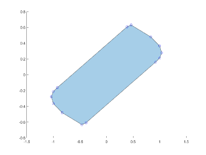
Figure 1: The figure shows the extremal polytope norm computed for Example 1.

3 Mixed (discrete-continuous) systems

3.1 Theoretical aspects

If all dwell times of a continuous-time switching system are fixed, then the latter is equivalent to a weighted system. But what if the dwell times of only a part of modes are fixed while the other dwell times have no restrictions? In this case our equivalent system includes both continuous and discrete part. This motives the following construction.

Let ${\cal{A}}=\{A_{1},\ldots,A_{m}\}$ be a finite family of $d\times d$ matrices equipped with positive weights ${\boldsymbol{\alpha}}=\{\alpha_{1},\ldots,\alpha_{m}\}$ and let ${\cal{B}}$ be a bounded set of $d\times d$ matrices. For every sequence of matrices $\{A(i)\}_{i\in{\mathbb{N}}}$, from the family ${\cal{A}}$, $\alpha(i)$ denotes the weight of $A(i)$.

Definition 3.1.

The mixed system associated with the triple $({\cal{A}},{\boldsymbol{\alpha}},{\cal{B}})$ is the linear switching system having the following set of trajectories. Consider any sequence $\bigl{\{}\,\bigl{(}\,(a_{i},b_{i})\,,A(i)\,\bigr{)}\,\bigr{\}}_{i\in D}$, where each $A(i)$ is a matrix from ${\cal{A}}$ and $(a_{i},b_{i})\subset{\mathbb{R}}_{+}$ an open interval of length $\alpha(i)$. This sequence may be infinite ($D={\mathbb{N}}$), finite ($D=\{1,\ldots,n\}$), or empty ($D=\emptyset$). The sequence of intervals increases, i.e., $b_{i}\leq a_{i+1}$ for each $i$. The union of those intervals is called a dark domain, its complement in ${\mathbb{R}}_{+}$ is called an active domain and denoted by ${\cal{T}}$. For any measurable function $B:\,{\cal{T}}\to{\cal{B}}$, we consider the system of differential and difference equations

(7) $$\left\{\begin{array}[]{cclcl}\dot{x}(t)&=&B(t)x(t)\,,&&t\in{\cal{T}},\\[2.84526pt] x(b_{i})&=&A(i)x(a_{i})\,,&&i\in D.\end{array}\right.$$

Every solution $x:{\cal{T}}\to{\mathbb{R}}^{d}$ of this system is called a trajectory of the mixed system $({\cal{A}},{\boldsymbol{\alpha}},{\cal{B}})$, whose associated switching law is given by the sequence $\bigl{\{}\,\bigl{(}\,(a_{i},b_{i})\,,A(i)\,\bigr{)}\,\bigr{\}}_{i\in D}$ together with the function $B:{\cal{T}}\to{\cal{B}}$. We use ${\it sw}$ to denote any such switching law and ${\cal{S}\cal{W}}$ for the set of all switching laws associated with $({\cal{A}},{\boldsymbol{\alpha}},{\cal{B}})$.

Clearly, the classical continuous and discrete-time switching systems are special cases of mixed systems.

Every trajectory of a mixed system is uniquely determined by the switching law ${\it sw}$ and by the initial point $x(0)$. The trajectory has its own active domain ${\cal{T}}={\cal{T}}({\it sw})$, where it is defined. Thus, for a mixed system, a trajectory is not a function from ${\mathbb{R}}_{+}$ to ${\mathbb{R}}^{d}$, but a function from a certain closed subset ${\cal{T}}\subset{\mathbb{R}}_{+}$ to ${\mathbb{R}}^{d}$. If $t\notin{\cal{T}}$, then $x(t)$ is not defined. The dark domain ${\mathbb{R}}_{+}\setminus{\cal{T}}$ consists of the union of the intervals $(a_{i},b_{i})$. The transfer of the trajectory from the state $x(a_{i})$ to $x(b_{i})=A(i)x(a_{i})$ is called a jump, and $a_{i}$ is a jump point. The set of all trajectories will be denoted by ${\cal{X}}$.

Remark 3.2.

Let $({\cal{A}},{\boldsymbol{\alpha}},{\cal{B}})$ be a mixed system. Then its set of switching laws ${\cal{S}}{\cal{W}}$ is shift-invariant and closed by concatenation on their active domains, i.e., given two switching laws ${\it sw}^{1}$ and ${\it sw}^{2}$ in ${\cal{S}}{\cal{W}}$ and a time $T\in{\cal{T}}({\it sw}^{1})$, one can concatenate the restriction to $[0,T)$ of ${\it sw}^{1}$ with ${\it sw}^{2}$, in such a way to provide a switching law ${\it sw}={\it sw}^{1}_{|[0,T)}\ast{\it sw}^{2}$ in ${\cal{S}}{\cal{W}}$.

Example 3.3.

An important special case of a mixed system is a continuous-time linear switching system $\dot{x}=B(t)x$, $t\in{\mathbb{R}}_{+}$, where for each $t$, the matrix $B(t)$ is from a finite set of matrices ${\cal{B}}=\{B_{1},\ldots,B_{n}\}$, and for several of them, say, for $B_{1},\ldots,B_{m}$, the dwell times are fixed. This means that each matrix $B_{i}$, $1\leq i\leq m,$ can be activated only for a time interval of a prescribed length $\alpha_{i}>0$ (or positive multiples of it). By setting $A_{i}=e^{\alpha_{i}B_{i}}$, $i\leq m$, we obtain a mixed system $({\cal{A}},{\boldsymbol{\alpha}},{\cal{B}})$ with ${\cal{A}}=\{A_{1},\ldots,A_{m}\}$, ${\boldsymbol{\alpha}}=\{\alpha_{1},\ldots,\alpha_{m}\}$, and ${\cal{B}}=\{B_{m+1},\ldots,B_{n}\}$. However, not every mixed system has this form, because not all matrices can be presented as matrix exponentials.

The definitions of stability and of Lyapunov exponent are directly extended to mixed systems.

Definition 3.4.

A mixed system $({\cal{A}},{\boldsymbol{\alpha}},{\cal{B}})$ is stable if every trajectory is bounded on its active domain. It is asymptotically stable if for every trajectory $x$, we have $x(t)\to 0$ as ${t\to\infty,\ t\in{\cal{T}}}$.

The previous definition makes sense since clearly ${\cal{T}}$ contains an increasing sequence of points tending to infinity.

Definition 3.5.

The Lyapunov exponent of a mixed system is the quantity

$$\sigma({\cal{A}},{\boldsymbol{\alpha}},{\cal{B}})\quad=\quad\inf\,\Bigl{\{}\beta\in{\mathbb{R}}\ \Bigr{|}\ \limsup_{t\to\infty,\ t\in{\cal{T}}}\frac{\ln(\|x(t)\|)}{t}\,\leq\,\beta\,,\ x\in{\cal{X}}\,\Bigr{\}}.$$

The properties of the Lyapunov exponent $\sigma$ are similar to those for the classical discrete-time or continuous-time linear switching systems. For example, one can easily establish the following “shift identity”: for every $\tau\in{\mathbb{R}}$, we have

(8) $$\sigma\,\Bigl{(}\delta_{\tau}^{\boldsymbol{\alpha}}({\cal{A}})\,,{\boldsymbol{\alpha}}\,,\,{\cal{B}}+\tau I\,\Bigr{)}\quad=\quad\tau\ +\ \sigma\Bigl{(}{\cal{A}},{\boldsymbol{\alpha}},{\cal{B}}\Bigr{)}\,.$$

In the following lemma, we prove a Fenichel type of result for mixed systems, namely that asymptotic stability and exponential stability are equivalent properties for a mixed system.

Lemma 3.6.

Let $({\cal{A}},{\boldsymbol{\alpha}},{\cal{B}})$ be a mixed system and define

$$\hat{\sigma}({\cal{A}},{\boldsymbol{\alpha}},{\cal{B}})=\inf\,\Bigl{\{}\beta\in{\mathbb{R}}\ \Bigr{|}\ \exists C>0\mbox{ s.t. }\|x(t)\|\leq Ce^{\beta t}\|x(0)\|\mbox{ for all }x\in{\cal{X}}\,,\ t\in{\cal{T}}\Bigr{\}}.$$

Then

a)

$\sigma({\cal{A}},{\boldsymbol{\alpha}},{\cal{B}})=\hat{\sigma}({\cal{A}},{\boldsymbol{\alpha}},{\cal{B}})$;

b)

$({\cal{A}},{\boldsymbol{\alpha}},{\cal{B}})$ is asymptotically stable if and only if $\sigma({\cal{A}},{\boldsymbol{\alpha}},{\cal{B}})<0$.

Before providing a proof, let us introduce the next definition.

Definition 3.7 (Interpolation of a trajectory of a mixed system).

Let $x:{\cal{T}}\to\mathbb{R}^{d}$ be a trajectory of a mixed system $({\cal{A}},{\boldsymbol{\alpha}},{\cal{B}})$ with active domain ${\cal{T}}$ and dark domain ${\mathbb{R}}_{+}\setminus{\cal{T}}$. The interpolation $\hat{x}$ of $x$ is the curve $\hat{x}:[0,\infty)\to\mathbb{R}^{d}$ defined as $\hat{x}=x$ on ${\cal{T}}$ and by linear interpolation on the dark domain, i.e., $\hat{x}(t)=x(a)+\frac{t-a}{b-a}(x(b)-x(a))$ for $t$ in a connected component $(a,b)$ of ${\mathbb{R}}_{+}\setminus{\cal{T}}$. We use $\widehat{{\cal{X}}}$ to denote the set of all interpolated trajectories.

It is clear that any interpolation $\hat{x}$ of a trajectory $x$ of a mixed system is continuous and piecewise $C^{1}$ with a derivative verifying the following property: there exists a positive constant $C$ only depending on $({\cal{A}},{\boldsymbol{\alpha}},{\cal{B}})$ such that $\|\dot{\hat{x}}(t)\|\leq C\|\hat{x}(t)\|$ for a.e. $t\in{\cal{T}}$ and $\|\dot{\hat{x}}(t)\|\leq C\|\hat{x}(a)\|$ if $t\in(a,b)$ for every connected component $(a,b)$ of ${\mathbb{R}}_{+}\setminus{\cal{T}}$. Based on such a property we deduce the following compactness result.

Lemma 3.8.

Let ${\cal{B}}$ be compact and convex and consider $K\subset{\mathbb{R}}^{d}$ compact. Then for every sequence $({\it sw}_{k})_{k\in\mathbb{N}}\subset{\cal S}{\cal W}$ and every sequence $(x_{k})_{k\in\mathbb{N}}\subset K$, there exist ${\it sw}\in{\cal S}{\cal W}$ and $x\in K$ such that, up to subsequence, $\hat{x}(\cdot;x_{k},{\it sw}_{k})\to\hat{x}(\cdot;x,{\it sw})$ uniformly on $[0,T]$ for every $T>0$. Moreover, for $T>0$, ${\cal{T}}({\it sw}_{k})\cap[0,T+1/k]\to{\cal{T}}({\it sw})\cap[0,T]$ in the sense of the Hausdorff distance.

Proof 3.9.

Let us start by noticing that, given $T>0$, up to subsequence, ${\cal{T}}({\it sw}_{k})\cap[0,T+1/k]$ converges to the complement in $[0,T]$ of a finite number of intervals of the type $(a,a+\alpha)\cap[0,T]$ with $\alpha\in{\boldsymbol{\alpha}}$, since the number of connected components of the dark domain ${\mathbb{R}}_{+}\setminus{\cal{T}}({\it sw}_{k})$ intersecting $[0,T]$ is uniformly bounded. By a diagonal argument, the convergence holds for every $T>0$.

Let us now deduce the first part of the statement from Arzelà–Ascoli theorem, by checking that the restrictions to $[0,T]$ of trajectories from $\widehat{{\cal{X}}}$ starting in $K$ form a closed, uniformly bounded and equicontinuous set. Uniform boundedness is clear from the finiteness of ${\cal{A}}$ and the boundedness of ${\cal{B}}$, while equicontinuity follows from the remark before the lemma. Finally, closedness is a consequence of the well-know corresponding property in the case ${\cal{A}}=\emptyset$ and the convergence up to subsequence of the active domains.

Proof 3.10 (Proof of Lemma 3.6).

It is clear that $\sigma({\cal{A}},{\boldsymbol{\alpha}},{\cal{B}})\leq\hat{\sigma}({\cal{A}},{\boldsymbol{\alpha}},{\cal{B}})$ and that $\sigma({\cal{A}},{\boldsymbol{\alpha}},{\cal{B}})<0$ implies asymptotic stability.

The lemma is proved if we show that asymptotic stability implies that $\hat{\sigma}({\cal{A}},{\boldsymbol{\alpha}},{\cal{B}})<0$. Indeed, by means of (8) and together with the trivial implication in Item a), this shows that if $\sigma({\cal{A}},{\boldsymbol{\alpha}},{\cal{B}})<\lambda$ for some $\lambda\in\mathbb{R}$, then $\hat{\sigma}({\cal{A}},{\boldsymbol{\alpha}},{\cal{B}})<\lambda$ is also true, that is, $\hat{\sigma}({\cal{A}},{\boldsymbol{\alpha}},{\cal{B}})\leq\sigma({\cal{A}},{\boldsymbol{\alpha}},{\cal{B}})$.

Let $S$ be the unit sphere of $\mathbb{R}^{d}$ for the norm $\|\cdot\|$. We claim that there exists a time $T>0$ such that, for every $x\in S$ and ${\it sw}\in{\cal S}{\cal W}$, one has $\|{x}(t;x,{\it sw})\|\leq 1/2$ for some $t\in[0,T]\cap{\cal{T}}({\it sw})$. Indeed, arguing by contradiction, one should have that for every $k\in\mathbb{N}$ there exist $x_{k}\in S$ and ${\it sw}_{k}\in{\cal S}{\cal W}$ such that

(9) $$\|{x}(t;x_{k},{\it sw}_{k})\|\geq 1/2$$

for every $t\in[0,k]\cap{\cal{T}}({\it sw}_{k})$. Denoting by $\overline{{\rm co}}({\cal{B}})$ the closure of the convex hull of ${\cal{B}}$, by Lemma 3.8 there exist a trajectory ${x}_{*}$ of $({\cal{A}},{\boldsymbol{\alpha}},\overline{{\rm co}}({\cal{B}}))$ with active domain ${\cal{T}}$ such that $\|{x}_{*}(t)\|\geq 1/2$ for every $t\in{\cal{T}}$. Hence $({\cal{A}},{\boldsymbol{\alpha}},\overline{{\rm co}}({\cal{B}}))$ is not asymptotically stable, which, by a standard approximation argument (see [17]), contradicts the asymptotic stability of $({\cal{A}},{\boldsymbol{\alpha}},{\cal{B}})$ and, thus, proves the claim.

One easily deduces from the claim and the shift-invariance property observed in Remark 3.2 that there exists $C>0$ such that $\|{x}(t)\|\leq C2^{-t/T}\|{x}(0)\|$ for every ${x}\in\widehat{{\cal{X}}}$ and every $t\in{\cal{T}}$, concluding the proof of the lemma.

The notions of non-defectiveness and irreducibility extend to mixed systems as follows.

Definition 3.11.

A mixed system $({\cal{A}},{\boldsymbol{\alpha}},{\cal{B}})$ is said to be

• non-defective if there exists a positive constant $C$ such that $\|x(t)\|\leq Ce^{\sigma t}\|x(0)\|$ for every $x\in{\cal{X}}$ and every $t\in{\cal{T}}$, where $\sigma=\sigma({\cal{A}},{\boldsymbol{\alpha}},{\cal{B}})$;

• irreducible if ${\cal{A}}\cup{\cal{B}}$ is irreducible.

Let us note that a trajectory of a mixed system may reach the origin at some time $\tilde{t}<\infty$, after which it stays at the origin forever. This situation is impossible for continuous-time systems, but for mixed systems it can happen, provided that one of the matrices $A_{j}$ is degenerate.

Given a trajectory $x(\cdot)$ of the mixed system and $f:{\mathbb{R}}^{d}\to{\mathbb{R}}_{+}$ positive define, we say that $f(x(t))$ strictly decreases in $t$ if $f(x(t_{1}))>f(x(t_{2}))$ for every $t_{1},t_{2}\in{\cal{T}}$ such that $t_{1}<t_{2}$ and $x(t_{1})\neq 0$. Thus, the value $f(x(t))$ decreases not on the whole ${\mathbb{R}}_{+}$, where it may not be defined, but on the active domain. Moreover, if the trajectory stabilizes at zero at some time $\tilde{t}$, then we require $f(x(t))$ to strictly decrease only for $t<\tilde{t}$.

We now formulate the main theorem on extremal and invariant norms for mixed systems.

Theorem 3.12.

Let $({\cal{A}},{\boldsymbol{\alpha}},{\cal{B}})$ be a mixed system and set $\sigma=\sigma({\cal{A}},{\boldsymbol{\alpha}},{\cal{B}})$. Then the following holds:

a) For $\lambda\in\mathbb{R}$, $\sigma<\lambda$ if and only if there exists a norm in ${\mathbb{R}}^{d}$ such that for every trajectory $x\in{\cal{X}}$, the function $\|e^{-\lambda t}x(t)\|$ strictly decreases on ${\cal{T}}$. In the corresponding operator norm, we have $\|A_{j}\|\,<\,e^{\alpha_{j}\lambda}\,,\,A_{j}\in{\cal{A}}$, and for each $x$ in the unit sphere of this norm, all vectors $(B-\lambda I)x,\,B\in{\cal{B}},$ starting at $x$, are directed inside the unit sphere (i.e., $\|x+\varepsilon(B-\lambda I)x\|<1$ for every $\varepsilon>0$ small enough).

b) If $({\cal{A}},{\boldsymbol{\alpha}},{\cal{B}})$ is non-defective, then it has an extremal norm, for which every trajectory possesses the property $\|x(t)\|\leq e^{\sigma t}\|x(0)\|,\,t\in{\cal{T}}$.

c) If $({\cal{A}},{\boldsymbol{\alpha}},{\cal{B}})$ is irreducible and ${\cal{B}}$ is compact and convex, then it possesses an invariant norm, for which all trajectories satisfy $\|x(t)\|\leq e^{\sigma t}\|x(0)\|,\,t\in{\cal{T}}$, and for every $x_{0}\in{\mathbb{R}}^{d}$ there exists a trajectory $\bar{x}$ starting at $x_{0}$ such that $\|\bar{x}(t)\|=e^{\sigma t}\|x_{0}\|$, $t\in{\cal{T}}$.

Item a) of Theorem 3.12, together with Item b) of Lemma 3.6, immediately implies the following.

Corollary 6.

A mixed system is asymptotically stable if and only if there exists a norm $\|\cdot\|$ in ${\mathbb{R}}^{d}$ such that for every trajectory $x\in{\cal{X}}$, $\|x(t)\|$ strictly decreases in $t$.

On the other hand, Item c) of Theorem 3.12 has the following geometrical interpretation.

Corollary 7.

Let $({\cal{A}},{\boldsymbol{\alpha}},{\cal{B}})$ be an irreducible mixed system with $\sigma({\cal{A}},{\boldsymbol{\alpha}},{\cal{B}})=0$ and $G$ be the unit ball of the invariant norm given in Item c) of Theorem 3.12. Then every trajectory starting in $G$ never leaves $G$. On the other hand, if ${\cal{B}}$ is compact and convex, then for every point $x_{0}$ in the boundary of $G$, there exists a trajectory that starts at $x_{0}$ and lies entirely on that boundary.

We next provide a proof of Theorem 3.12.

Proof 3.13 (Proof of Theorem 3.12).

We split the proof into four steps. First we construct a special positively-homogeneous monotone convex functional $\varphi$ (Step 1) and prove that it is actually a norm in ${\mathbb{R}}^{d}$ when it is finite (Step 2). As a consequence, we deduce Items a) and b). In Step 3 we show that irreducibility implies non-defectiveness, and so $\varphi$ is an extremal norm for irreducible systems. Finally, in Step 4, based on $\varphi$ we construct an invariant norm $w$. In view of (8) it suffices to consider the case $\lambda=0$ in item a) and $\sigma=0$ in items b) and c). We can also, without loss of generality, assume that ${\cal{B}}\not=\emptyset$, since otherwise $({\cal{A}},{\boldsymbol{\alpha}},{\cal{B}})$ is a weighted system, for which Theorem 2.10 applies.

Step 1. For arbitrary $t\geq 0$ and $z\in{\mathbb{R}}^{d}$, denote

$$\ell(z,t)\ =\ \sup\,\Bigl{\{}\,\|x(t)\|\,\mid\quad x\in{\cal{X}}\,,\,x(0)=z\,,\,t\in{\cal{T}}\Bigr{\}}\ .$$

The supremum is taken over those trajectories whose active domain contains $t$. The set of such trajectories is nonempty, since we are assuming that ${\cal{B}}\not=\emptyset$.

For every fixed $t$, the function $\ell(\cdot,t)$ is a seminorm on ${\mathbb{R}}^{d}$, i.e., it is positively homogeneous and convex, as a supremum of homogeneous convex functions. The function

$$\varphi(z)=\sup\limits_{t\in{\mathbb{R}}_{+}}\ell(z,t)$$

is, therefore, also a seminorm as a supremum of seminorms. Moreover, $\varphi(z)\geq\ell(z,0)=\|z\|$, hence $\varphi(z)$ is strictly positive, whenever $z\neq 0$. For every trajectory $x(t)$ the function $\varphi\bigl{(}x(t)\bigr{)}$ is non-increasing in $t$ on the set ${\cal{T}}$, by the concatenation property presented in Remark 3.2. Thus, if $\varphi(z)<+\infty$ for all $z$, then $\varphi$ is a norm which is non-decreasing along every trajectory of the system.

Step 2. If $\sigma<0$, then $\sigma<-\varepsilon$ for some positive $\varepsilon$. Consider the shifted system $(\delta^{\boldsymbol{\alpha}}_{\varepsilon}({\cal{A}}),{\boldsymbol{\alpha}},{\cal{B}}+\varepsilon I)$ and denote by $\varphi_{\varepsilon}$ the corresponding function $\varphi$ for this system.

Thanks to (8) and to Item a) of Lemma 3.6, all trajectories of $(\delta^{\boldsymbol{\alpha}}_{\varepsilon}({\cal{A}}),{\boldsymbol{\alpha}},{\cal{B}}+\varepsilon I)$ are uniformly bounded, and hence $\varphi_{\varepsilon}(z)<+\infty$ for each $z\in{\mathbb{R}}^{d}$. Therefore, $\varphi_{\varepsilon}$ is a norm, which is non-decreasing along any trajectory of the shifted system. On the other hand, every trajectory of the shifted system has the form $e^{-\varepsilon t}x(t)$, where $x\in{\cal{X}}$. For every $t_{1},t_{2}\in{\cal{T}}$ such that $t_{1}<t_{2}$, we have $\|e^{\varepsilon t_{1}}x(t_{1})\|\geq\|e^{\varepsilon t_{2}}x(t_{2})\|$. Thus, $\|x(t_{2})\|\leq e^{\varepsilon(t_{1}-t_{2})}\|x(t_{1})\|$. Hence, the norm $\varphi_{\varepsilon}$ strictly decreases along every trajectory $x\in{\cal{X}}$.

Now consider a new norm $\|\cdot\|=\varphi_{\varepsilon}(\cdot)$. For arbitrary $x_{0}\neq 0$ and $A_{j}\in{\cal{A}}$, take a switching law with $a_{1}=0,A(1)=A_{j}$, and take an arbitrary trajectory starting at $x_{0}$. We have $\|A_{j}x_{0}\|=\|x(b_{1})\|<\|x(a_{1})\|=\|x_{0}\|$. Thus, $\|A_{j}x_{0}\|<\|x_{0}\|$. Since this is true for all $x_{0}\neq 0$, we see that $\|A_{j}\|<1$. This proves the first property from a). On the other hand, as shown in [24, 25] each norm that decreases along any trajectory possesses the second property from a): for every $x$ such that $\|x\|=1$, all the vectors $Bx,\,B\in{\cal{B}}$, starting at $x$ are directed inside the unit sphere. This completes the proof of a).

To prove b) it suffices to observe that if the system is non-defective and $\sigma=0$, then $\varphi(x)<+\infty$ for all $x$. Hence, $\varphi$ is a desired extremal norm, which in non-decreasing along any trajectory $x\in{\cal{X}}$. This concludes the proof of b).

Step 3. Let us now tackle Item c). We begin by proving that if the system is irreducible, then $\varphi(x)<+\infty$ for all $x$, and so $\varphi$ is a norm. Denote by ${\cal{L}}$ the set of points $x\in{\mathbb{R}}^{d}$ such that $\varphi(x)<+\infty$. Since $\varphi$ is convex and homogeneous, it follows that ${\cal{L}}$ is a linear subspace of ${\mathbb{R}}^{d}$. Let us show that ${\cal{L}}$ is an invariant subspace for all operators from ${\cal{A}}$ and from ${\cal{B}}$. For every $z\in{\cal{L}}$, each trajectory starting at $z$ is bounded, hence each trajectory starting at $Az$, $A\in{\cal{A}}$, is bounded as well, as a part of the trajectory starting at $z$. Hence, $Az\in{\cal{L}}$ and so ${\cal{L}}$ is a common invariant subspace for the family ${\cal{A}}$. Similarly, for every $z\in{\cal{L}}$, $B\in{\cal{B}}$, and $t\geq 0$, $e^{tB}(z)$ is in ${\cal{L}}$, from which we deduce that the tangent vector $Bz$ is also in ${\cal{L}}$. Thus, ${\cal{L}}$ is a common invariant subspace for both ${\cal{A}}$ and ${\cal{B}}$. From the irreducibility it follows that either ${\cal{L}}={\mathbb{R}}^{d}$ (in which case $\varphi$ is a norm) or ${\cal{L}}=\{0\}$. It remains to show that the latter is impossible.

Consider the unit sphere $S=\{x\in{\mathbb{R}}^{d}\ |\ \|x\|=1\}$. If ${\cal{L}}=\{0\}$, then $\varphi(x)=+\infty$ for all $x\in S$. For every natural $n$ denote by ${\cal{H}}_{\,n}$ the set of points $z\in S$ for which there exist a trajectory starting at $z$ and a time $T=T(z)\leq n$ in the corresponding active domain ${\cal{T}}$ such that $\|x(T)\|>2$. Clearly, $\cup_{n=1}^{\infty}{\cal{H}}_{\,n}\,=\,S$. Since each ${\cal{H}}_{\,n}$ is open, the compactness of $S$ implies the existence of a finite subcovering, i.e., the existence of a natural $N$ such that $\cup_{n=1}^{N}{\cal{H}}_{\,n}\,=\,S$. Equivalently, $T(z)\leq N$ for all $z\in S$. Thus, starting from an arbitrary point $x_{0}\in S$ one can consequently build a trajectory $x\in{\cal{X}}$ and an increasing sequence $(t_{k})_{k\in\mathbb{N}}$ in ${\cal{T}}$ such that $\|x({t_{k+1}})\|\,>\,2\|x({t_{k}})\|$ and $|t_{k+1}-t_{k}|\leq N$ for all $k$. For this trajectory, $\|x(t_{n})\|\,>\,2^{n}$ and $t_{n}\leq nN$, hence $\|x(t_{n})\|\,>\,e^{t_{n}\ln 2/N}$. Therefore, $\sigma\geq\frac{\ln 2}{N}>0$, which contradicts the assumption. The contradiction argument allows to conclude that ${\cal{L}}={\mathbb{R}}^{d}$ and $\varphi$ is a norm.

Step 4. We have found a norm $\varphi$ which is non-increasing on the active domain along every trajectory $x\in{\cal{X}}$. By convexity of $\varphi$, this also implies that $\varphi(\hat{x}(t))\leq\varphi(\hat{x}(0))$ for every trajectory $\hat{x}\in\widehat{{\cal{X}}}$ and every $t\geq 0$. Define, for every $x\in\mathbb{R}^{d}$,

$$w(x)=\limsup_{t\to\infty}\sup_{{\it sw}\in{\cal{S}}{\cal{W}}}\varphi(\hat{x}(t;x,{\it sw})).$$

The finiteness of $w$ follows from the monotonicity of $\varphi$. Notice that, by Remark 3.2,

(10) $$w(x(t;x,{\it sw}))\leq w(x),\qquad{\it sw}\in{\cal{S}}{\cal{W}},\;t\in{\cal{T}}({\it sw}).$$

We claim that $w$ is a norm. Homogeneity is obvious and subadditivity follows form the inequality

$$\varphi(\hat{x}(t;x+y,{\it sw}))\leq\varphi(\hat{x}(t;x,{\it sw}))+\varphi(\hat{x}(t;y,{\it sw})),\ \quad{\it sw}\in{\cal{S}}{\cal{W}},\ t\geq 0.$$

Let us assume by contradiction that $w(x)=0$ for some $x\neq 0$. It follows from (10) that $w(x(t;x,{\it sw}))=0$ for all ${\it sw}\in{\cal{S}}{\cal{W}}$ and $t\in{\cal{T}}({\it sw})$. Since, moreover, the linear space generated by $\{x(t;x,{\it sw})\mid{\it sw}\in{\cal{S}}{\cal{W}},\;t\in{\cal{T}}({\it sw})\}$, is invariant for ${\cal{A}}\cup{\cal{B}}$, then it is equal to $\mathbb{R}^{d}$, which implies that $w\equiv 0$ on $\mathbb{R}^{d}$. It follows from Item b) of Lemma 3.6 that $\sigma({\cal{A}},{\boldsymbol{\alpha}},{\cal{B}})<0$, leading to a contradiction. This concludes the proof that $w$ is a norm.

Take now $x\in\mathbb{R}^{d}$ and consider two sequences $({\it sw}_{k})_{k\in\mathbb{N}}\subset{\cal S}{\cal W}$ and $(t_{k})_{k\in\mathbb{N}}\subset{\mathbb{R}}_{+}$ such that $t_{k}\to\infty$ as $k\to\infty$ and

$$w(x)=\lim_{k\to\infty}\varphi(\hat{x}(t_{k};x,{\it sw}_{k})).$$

Since $\varphi$ is non-increasing along trajectories, we have that

(11) $$\liminf_{k\to\infty}\min_{t\in[0,t_{k}]\cap{\cal{T}}({\it sw}_{k})}\varphi(x(t;x,{\it sw}_{k}))\geq w(x).$$

By Lemma 3.8, there exists ${\it sw}\in{\cal S}{\cal W}$ such that, up to subsequence, $\hat{x}(\cdot;x,{\it sw}_{k})$ converges to $\hat{x}(\cdot;x,{\it sw})$ uniformly on all compacts of ${\mathbb{R}}_{+}$. Moreover, ${\cal{T}}({\it sw}_{k})$ converges to ${\cal{T}}({\it sw})$ on compact intervals in the sense guaranteed by Lemma 3.8. Together with (11), this implies that

$$\liminf_{t\to\infty,\;t\in{\cal{T}}({\it sw})}\varphi(x(t;x,{\it sw}))\geq w(x).$$

Hence, by definition of $w$, $w(x)=\lim_{t\to\infty,\;t\in{\cal{T}}({\it sw})}\varphi(x(t;x,{\it sw}))$. We conclude the proof that $w$ is an invariant norm by deducing from (10) that $w(x(t;x,{\it sw}))=w(x)$ for every $t\in{\cal{T}}({\it sw})$.

Having proved the existence theorem for extremal and invariant norms we are now able to approximate the Lyapunov exponent numerically by constructing polytopic Lyapunov functions.

3.2 The algorithm for mixed systems

One of the methods to prove stability of mixed systems is by discretization. First we assume that ${\cal{B}}$ is finite.

It is well known that the joint spectral radius of a compact set ${\cal{B}}$ of matrices is the same as that of its convex hull ${\rm co}({\cal{B}})$. If this is finitely generated, i.e., ${\rm co}({\cal{B}})={\rm co}\left(\{B_{1},B_{2},\ldots,B_{m}\}\right)$ then we can apply our algorithm. If this is not the case, one possibility would be that of finding a nearby polyhedron containing ${\rm co}({\cal{B}})$ and apply the algorithm to the family given by the vertexes of this polyhedral set. If the set is ${\varepsilon}$-close to ${\cal{B}}$ then the computed joint spectral radius is ${\varepsilon}$-close to the joint spectral radius $\rho\left({\rm co}({\cal{B}})\right)=\rho\left({\cal{B}}\right)$.

The idea is that of constraining (7) by imposing that the time instants at which switching is allowed (the switching instants) for the free matrices (those belonging to ${\cal{B}}$) are multiple of a small time-duration $\tau$.

This procedure gives rise to a weighted system $({\cal C}_{\tau},\gamma_{\tau})$ whose corresponding modes are the elements of ${\cal{A}}$ and those of ${\cal{B}}_{\tau}=\{{\rm e}^{\tau B}\mid B\in{\cal{B}}\}$, i.e., ${\cal C}_{\tau}={\cal{A}}\cup{\cal{B}}_{\tau}$. The weight vector $\gamma_{\tau}$ is obtained associating with any element $A_{i}\in{\cal{A}}$ its corresponding $\alpha_{i}$ from ${\boldsymbol{\alpha}}$ and with any matrix in ${\cal{B}}_{\tau}$ the weight $\tau$.

We recall that Algorithm 1 tries to find a s.m.p. $\Pi_{\tau}=C(k)\cdots C(1)$, with $C(1),\dots,C(k)\in{\cal C}_{\tau}$, such that $\rho({{\cal C}}_{\tau},\gamma_{\tau})=\rho(\Pi_{\tau})^{\frac{1}{|\Pi_{\tau}|}}$. If this is done, then the weighted joint spectral radius is found.

3.3 Lower and upper bounds for the Lyapunov exponent

Note that, for any $\tau>0$ and for an arbitrary product $\Pi$ of matrices from ${{\cal C}}_{\tau}$, the Lyapunov exponent $\sigma({\cal{A}},{\boldsymbol{\alpha}},{\cal{B}})$ of system (7) is bounded below by the quantity

(12) $$\beta(\Pi)\ =\ \frac{1}{|\Pi|}\log\left(\rho(\Pi)\right).$$

Choosing the product with the biggest $\beta(\Pi)$, we find the best lower bound for the Lyapunov exponent. If Algorithm 1 finds the s.m.p. $\Pi_{\tau}$, then this product provides this best lower bound. Using the short notation $\beta(\tau)=\beta(\Pi_{\tau})$, we get

(13) $$\beta(\tau)\ \leq\ \sigma({\cal{A}},{\boldsymbol{\alpha}},{\cal{B}})\,.$$

Similarly to [12], an upper bound to $\sigma({\cal{A}},{\boldsymbol{\alpha}},{\cal{B}})$ is found as follows. For an arbitrary polytope $P\subset{\mathbb{R}}^{d}$ symmetric about the origin and for the weighted family $(C_{\tau},\gamma_{\tau})$, we define the value $\mu({\cal{B}},P)\,=\,\mu(P)$ as

(14) $$\mu(P) = \inf\ \Bigl{\{}\mu\in{\mathbb{R}}\mid\mbox{for each vertex}\ v\in P\ \mbox{and}\ B\in{\cal{B}},\Bigr{.}$$

$$\Bigl{.}\qquad\mbox{the vector}\ (B-\mu I)v\ \mbox{is directed inside}\,P\,\Bigr{\}}\,.$$

For the extremal polytope $P_{\tau}$ computed by Algorithm 1 we use the short notation $\mu(P_{\tau})=\mu(\tau)$. The following simple observation is crucial for the further results.

Proposition 8.

Let ${\cal{B}}$ be finite and $\tau>0$. Then for an arbitrary symmetric polytope $P$ and for arbitrary product $\Pi$ of matrices from the weighted family $(C_{\tau},\gamma_{\tau})$, we have

(15) $$\beta(\Pi)\ \leq\ \sigma({\cal{A}},{\boldsymbol{\alpha}},{\cal{B}})\ \leq\ \mu(P)\,.$$

In particular,

(16) $$\beta(\tau)\ \leq\ \sigma({\cal{A}},{\boldsymbol{\alpha}},{\cal{B}})\ \leq\ \mu(\tau)\,.$$

Proof 3.14.

The proof is completely analogous to the one given in [12] for classical switching systems.

If, for a polytope $P$, we have $e^{\,\tau\,B}\,P\,\subset\,\lambda^{\tau}\,P\,,\ B\in{\cal{B}}$, as well as $A_{i}P\,\subset\,\lambda^{\alpha_{i}}\,P\,,\ A_{i}\in{\cal{A}}$, then $\lambda\geq\rho({\cal C}_{\tau},\gamma_{\tau})$. Clearly, if we have an extremal polytope $P_{\tau}$ available, then we also know the value of the corresponding weighted joint spectral radius. In some cases, however, the extremality property is a too strong requirement, and computing the invariant polytope may take too much time. However, to estimate the Lyapunov exponent the following weaker version of extremality suffices:

Definition 3.15.

Given ${\varepsilon}\geq 0$, a polytope $P$ is called ${\varepsilon}$-extremal for $({\cal C}_{\tau},\gamma_{\tau})$ if

$$e^{\tau B}\,P\ \subset\ e^{\tau{\varepsilon}}\,\rho(C_{\tau},\gamma_{\tau})^{\tau}\,P\,,\qquad B\in{\cal{B}}\,,$$

and

$$A_{i}\,P\ \subset\ e^{\alpha_{i}{\varepsilon}}\,\rho(C_{\tau},\gamma_{\tau})^{\alpha_{i}}\,P\,,\qquad A_{i}\in{\cal{A}}\,.$$

When $P=P_{\tau}$ is extremal, the double inequality (16) localizes the Lyapunov exponent to the segment $[\beta(\tau)\,,\,\mu(\tau)]$. The length of this segment does not exceed a linear function of $\tau$. So, the precision of the estimate (16) is not worse than $C\tau$. The following theorem considers a more general case, when the polytope $P$ is not necessarily extremal but only ${\varepsilon}$-extremal.

Theorem 3.16.

For every finite irreducible mixed system $({\cal{A}},\alpha,{\cal{B}})$, there exists a positive constant $C$ such that for all $\,{\varepsilon}\geq 0$ and $\tau$ such that the family ${\cal C}_{\tau}$ is irreducible, we have

$$\mu(P)\ -\ \beta(\tau)\ \leq\ C\tau\,+\,{\varepsilon}\,,$$

whenever $P$ is an ${\varepsilon}$-extremal polytope for $({\cal C}_{\tau},\gamma_{\tau})$.

Thus, by inequality (15), every discretization time $\tau>0$ gives the lower bound $\beta(\Pi)$ for the Lyapunov exponent, and that discretization time with an ${\varepsilon}$-extremal polytope $P$ gives the upper bound $\mu(P)$. Theorem 3.16 ensures that at least in case $\Pi=\Pi_{\tau}$, the precision of these bounds is linear in $\tau$ and ${\varepsilon}$. In particular, for ${\varepsilon}=0$, we have the following.

Corollary 9.

If the polytope $P_{\tau}$ is extremal for $({\cal C}_{\tau},\gamma_{\tau})$, then $\mu(\tau)-\beta(\tau)\,\leq\,C\tau$.

Remark 3.17.

If one succeed in finding a “proper” polytope $P$ and a product $\Pi$ for which the difference $\mu(P)-\beta(\Pi)$ is small, then we have an a posteriori estimate (15) for the Lyapunov exponent. Theorem 3.16 shows that at least in the case when $P$ is $\varepsilon$-extremal and $\Pi$ is an s.m.p. the precision of this estimate decays linearly with $\tau$. In most of practical cases this estimate behaves even better.

Proposition 8 and Theorem 3.16 suggest the following method of approximate computation of the Lyapunov exponent $\sigma({\cal{A}},\alpha,{\cal{B}})$:

1) choose a discretization time $\tau>0$, and compute the weighted joint spectral radius $\rho({\cal C}_{\tau},\gamma_{\tau})$;

2) choose ${\varepsilon}\geq 0$ and construct an ${\varepsilon}$-extremal polytope $P$ for $({\cal C}_{\tau},\gamma_{\tau})$ (if ${\varepsilon}=0$ we intend an extremal polytope).

Then we localize the Lyapunov exponent $\sigma({\cal{A}},\alpha,{\cal{B}})$ on the segment $[\beta(\tau),\mu(P)]$, whose length tends to zero with a linear rate in $\tau$ and ${\varepsilon}$ as $\tau,{\varepsilon}\to 0$.

If we consider a product $\Pi$ which is not an s.m.p. then we have to replace $\beta(\tau)$ by $\beta(\Pi)$. Let us recall that for every product $\Pi$, $\beta(\Pi)\leq\beta(\tau)$. Therefore if $\Pi$ is not an s.m.p. then the lower bound can be worse than the optimal one considered in Theorem 3.16. In such case linear convergence as $\tau\rightarrow 0$ is not guaranteed. In practice nevertheless the difference $\mu(P)-\beta(\Pi)$ can always be made sufficiently small to provide a satisfactory approximation of the Lyapunov exponent.

Deriving the lower and upper bounds for the Lyapunov exponent. Thus, the first part of the algorithm produces an ${\varepsilon}$-extremal polytope $P$. We compute $\mu(P)$ by definition, as the infimum of those numbers $\mu$ such that the vector $(B-\mu I)v$ is directed inside $P$, for each vertex $v\in P$ and for every $B\in{\cal{B}}$. This is done by taking a small $\delta>0$ and solving the following LP problem:

$$\left\{\begin{array}[]{l}\mu\ \to\ \inf\\ v+\delta(B-\mu I)v\,\in\,P,\\ \,v\quad{\rm vertex\ of}\quad P,\ B\in{\cal{B}}\,.\end{array}\right.$$

Thus, as a result of Algorithms 1 and 2, we obtain the lower bound $\beta(\tau)$ and the upper bound $\mu(P)$ for the Lyapunov exponent. The polytope $P$ identifies the Lyapunov norm for the family. If $\mu(P)<0$, then we conclude that the system is asymptotically stable and its joint Lyapunov function has the polytope $P$ as unit ball.

Data: ${\cal{B}}=\{B_{1},\dots,B_{M}\}$, $P,V$ (system of vertices of $P=\mathrm{absco}(V)$, $\delta$ (small positive stepsize)

Result: $\mu(P)$

begin

       for $i=1,\ldots,M$ do

            1 Solve the LP problems (w.r.t. $\{t_{v},s_{v}\}$, $\mu_{i}$)

(20) $$\begin{array}[]{rl}\min&\mu_{i}\\[2.84544pt] {\rm s.t.}&v+\delta(B_{i}-\mu_{i}I)v=\sum\limits_{w\in{\cal{V}}}\,t_{w}\,w-s_{w}\,w\quad\forall v\in V\\[2.84544pt] {\rm and}&\sum\limits_{w\in V}\,t_{w}+s_{w}\leq 1,\qquad t_{w},s_{w}\geq 0\quad\forall w\in V\end{array}$$

      2Return $\mu(P):=\max\limits_{1\leq i\leq m}\mu_{i}$

      

Algorithm 2 Algorithm for computing the best upper bound $\mu(P)$

Example 3.18.

Let ${{\cal{A}}}=\{A_{1}\}$ with $\alpha_{1}=1$ and ${{\cal{B}}}=\{B_{1},B_{2}\}$ with

$$A_{1}=\left(\begin{array}[]{rr}0&-\frac{7}{5}\\ \frac{7}{5}&0\end{array}\right),\quad B_{1}=\log\left(\left(\begin{array}[]{rr}1&1\\ -1&1\end{array}\right)\right),\quad B_{2}=\log\left(\left(\begin{array}[]{rr}1&1\\ -1&0\end{array}\right)\right).$$

For $\tau=1$ we set exactly ${\cal C}_{\tau}=$ $\{A_{1},e^{B_{1}},e^{B_{2}}\}$ and $\gamma_{\tau}=(1,1,1)$.

By means of Algorithm 1 we are able to prove that the product of degree equal to $5$,

$$\Pi=e^{B_{2}}A_{1}e^{B_{1}}e^{B_{2}}A_{1}$$

is spectrum maximizing and apply Algorithm 1 with $C_{1}=A_{1}/\rho,C_{2}=e^{B_{1}}/\rho,C_{3}=e^{B_{2}}/\rho$, where $\rho=\rho({\cal C}_{\tau},\gamma_{\tau})$. As a result we obtain the polytope norm in Figure 2 whose unit ball $P$ is a polytope with $16$ vertices.

Applying Algorithm 2 we obtain the optimal shift $\mu(P)\approx 0.65$, so that we have the estimate

$$\beta(\tau)=0.38\ldots\leq\sigma({\cal{A}},{\boldsymbol{\alpha}},{\cal{B}})\leq 1.03\ldots=\mu(P_{\tau}).$$

Figure 2 illustrates the fact that the computed polytope $P$ is positively invariant for the shifted family ${\cal{B}}-\mu(P)I$.

In order to increase the accuracy of the computation one has to reduce $\tau$.

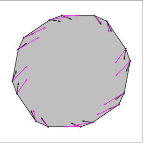
Figure 2: The figure shows the extremal polytope norm computed for Example 3.18.

4 Mixed systems on graphs

Recently many authors introduced and analysed constrained discrete-time switching systems, where not all switching laws are possible but only those satisfying certain stationary constraints [8, 19, 27, 28, 29, 32]. The concept slightly varies in different papers. One of the most general forms was considered in [7]. We describe the main construction, adapted to weighted systems (in [7] this was done for the usual discrete systems, i.e., with unit weights). Then we extend it to mixed systems.

4.1 Discrete weighted systems on graphs

Consider a directed strongly connected multigraph $G$ with $n$ vertices $g_{1},\ldots,g_{n}$. Sometimes, the vertices will be denoted by their indices. With each vertex $i$ we associate a linear space $L_{i}$ of dimension $d_{i}<\infty$. If the converse is not stated, we assume $d_{i}\geq 1$. The set of spaces $L_{1},\ldots,L_{n}$ is denoted by ${\cal{L}}$. For each vertices $i,j\in G$ (possibly coinciding), there is a set ${\cal{A}}_{ji}$ (possibly empty) of edges from $i$ to $j$. Each edge from ${\cal{A}}_{ji}$ is identified with a linear operator $A_{ji}:\,L_{i}\to L_{j}$ that has its weight $\alpha_{ji}>0$. Thus, we have a family of spaces ${\cal{L}}$ and a family of operators-edges ${\cal{A}}=\cup_{i,j}{\cal{A}}_{ji}$ that act between these spaces according to the multigraph $G$ and have weights ${\boldsymbol{\alpha}}=\{\alpha_{ji}\}_{i,j}$. We obtain a system $\,\xi=(G,{\cal{L}},{\cal{A}},{\boldsymbol{\alpha}})$ made of the multigraph, the spaces, the operators, and their weights. A path $\omega$ on the multigraph $G$ is a sequence of connected subsequent edges, its total weight (the sum of weights of edges) is denoted by $|\omega|$. With every path $\omega$ along vertices $i_{1}\rightarrow i_{2}\rightarrow\cdots\rightarrow i_{k+1}$ that consists of edges (operators) $A_{i_{s+1}i_{s}}\in{\cal{A}}_{i_{s+1}i_{s}},\,s=1,\ldots,k$, we associate the corresponding product (composition) of operators $\Pi_{\omega}=A_{i_{k+1}i_{k}}\cdots A_{i_{2}i_{1}}$. Note that $|\omega|=\alpha_{i_{k+1}i_{k}}+\cdots+\alpha_{i_{2}i_{1}}$. Let us emphasize that a path is not a sequence of vertices but edges. If $G$ is a graph, then any path is uniquely defined by the sequence of its vertices, if $G$ is a multigraph, then there may be many paths corresponding to the same sequence of vertices. If the path is closed ($i_{1}=i_{k+1}$), then $\Pi_{\omega}$ maps the space $L_{i_{1}}$ to itself. In this case $\Pi_{\omega}$ is given by a square matrix, and possesses eigenvalues, eigenvectors and a spectral radius $\rho(\Pi_{\omega})$. The set of all closed paths will be denoted by ${\cal C}(G)$. For an arbitrary $\omega\in{\cal C}(G)$ we denote by $\omega^{k}=\omega\cdots\omega$ the $k$th power of $\omega$.

In what follows we assume that all the sets ${\cal{A}}_{ji}$ are finite.

Now we recall the concept of multinorm introduced in [27] and adopted to arbitrary multigraph with arbitrary linear spaces in [7].

Definition 4.1.

If every space $L_{i}$ on the multigraph $G$ is equipped with a norm $\|\cdot\|_{i}$, then the collection of norms $\|\cdot\|_{i},\,i=1,\ldots,n$, is called a multinorm. The norm of an operator $A_{ji}\in{\cal{A}}_{ji}$ is defined as $\,\|A_{ji}\|\,=\sup\limits_{x\in L_{i},\|x\|_{i}=1}\|A_{ji}x\|_{j}$.

Note that the notation $\|x\|_{i}$ assumes that $x\in L_{i}$. In the sequel we suppose that the multigraph $G$ is equipped with some multinorm $\{\|\cdot\|_{i}\}_{i=1}^{n}$. We denote that multinorm by $\|\cdot\|$ and sometimes use the short notation $\|x\|=\|x\|_{i}$ for $x\in L_{i}$, that is, we drop the index of the norm if it is clear to which space $L_{i}$ the point $x$ belongs.

For a given $x_{0}\in L_{i}$ and for an infinite path $\omega$ starting at the vertex $i$, we consider the trajectory $\{x_{k}\}_{k\geq 0}$ of the system along this path. Here $x_{k}=\Pi_{\,\omega_{k}}\,x_{0}$, where $\omega_{k}$ is the prefix of $\omega$ of length $k$.

As usual, the system $\xi$ is called stable if every its trajectory is bounded. It is called asymptotically stable if every trajectory tends to zero as $\,k\to\infty$.

As for unconstrained weighted systems, the asymptotic behaviour is measured in terms of the weighted joint spectral radius, which in this case is defined as follows:

(22) $$\rho(\xi)\ =\ \lim_{k\to\infty}\,\max_{{\rm length}(\omega)=k}\|\Pi_{\omega}\|^{\,1/|\omega|}\,.$$

Thus, among all paths on $G$ of length $k$ we take one with the maximal value $\|\Pi_{\omega}\|^{\,1/|\omega|}$, then the limit of this value as $k\to\infty$ is the joint spectral radius. This limit always exists, as it can be proved following the same arguments as in Lemma 2.1.

A system is asymptotically stable precisely when there exists a multinorm $\|\cdot\|=\{\|\cdot\|_{i}\}_{i=1}^{n}$ decreasing along every trajectory. This means that the norms of all operators $A_{ji}$ are strictly less than one.

The concepts of extremal and invariant multinorms [27, 7] are also very similar to the corresponding norms. A multinorm $\|\cdot\|=\{\|\cdot\|_{i}\}_{i=1}^{n}$ is extremal if for every $i$ and $x\in L_{i}$, we have

(23) $$\max_{A_{ji}\in{\cal{A}}_{ji},\,j=1,\ldots,n}\,\rho(\xi)^{\,-\alpha_{ji}}\,\|A_{ji}x\|_{j}\ \leq\ \|x\|_{i}\,.$$

A multinorm is called invariant if for every $i=1,\ldots,n$ and $x\in L_{i}$, we have

(24) $$\max_{A_{ji}\in{\cal{A}}_{ji},\,j=1,\ldots,n}\,\rho(\xi)^{\,-\alpha_{ji}}\,\|A_{ji}x\|_{j}\ =\ \|x\|_{i}\,.$$

Thus, up to the normalization where one replaces every $A_{ji}$ by $\rho^{\,-\alpha_{ji}}A_{ji}$, an invariant multinorm is non-increasing along every trajectory, and for every $i$ and for every starting point $x_{i}\in L_{i}$, there exists an infinite trajectory $x_{i}=x(0)\to x(1)\to x(2)\to\cdots$ such that $\|x(0)\|=\|x(1)\|=\|x(2)\|=\cdots$.

The existence of invariant and of extremal multinorms was proved in [7] under the same assumptions as in Theorem 2.6. The algorithm constructing extremal polytope multinorms (when each norm $\|\cdot\|_{i}$ in the space $L_{i}$ is defined by a convex polytope $P_{i}$) was presented in the same paper. In examples and in statistics of numerical experiments it was shown that the algorithm is able to find precisely the joint spectral radius for a vast majority of constrained systems for reasonable time in dimensions up to $20$. For positive systems, it works much faster and is applicable in higher dimensions (several hundreds). It is interesting that the case of reducible system, when all operators share a common subspace, being very rare for unconstrained systems, becomes usual, or even generic for system on graphs. That is why a special procedure of reducibility was elaborated in [7].

4.2 Mixed systems on graphs

The constrained systems or systems on graphs appeared almost simultaneously in several works. All of them deal with discrete-time systems. To the best of our knowledge, there is no reasonable concept of a continuous-time system on a graph. Indeed, the existence of several spaces (vertices) between which the system can be transferred can naturally be realized in the discrete-time model, but any extension to continuous time seems hardly possible. Nevertheless, mixed system can be realized on graphs and for them various type of constraints can be introduced.

Let us have an arbitrary (discrete-time) system $(G,{\cal{L}},{\cal{A}},{\boldsymbol{\alpha}})$ on a multigraph $G$, with the spaces ${\cal{L}}=\{L_{1},\ldots,L_{n}\}$, operators ${\cal{A}}=\{A_{ji}\}$, and their weights ${\boldsymbol{\alpha}}=\{\alpha_{ji}\}$. Let us in addition have a family ${\cal{B}}=\{{\cal{B}}_{1},\ldots,{\cal{B}}_{n}\}$, where each ${\cal{B}}_{i}$ is a bounded set of operators acting on the space $L_{i}$. This identifies a mixed (discrete-continuous) system $\xi=(G,{\cal{L}},{\cal{A}},{\boldsymbol{\alpha}},{\cal{B}})$ on the multigraph $G$. A trajectory of this system along an infinite path $\omega:\,i_{1}\to i_{2}\to\ldots$ is a solution of the system of equations on the spaces $L_{i_{k}}$:

(25) $$\dot{x}(t)\,=\,B_{k}(t)x(t)\ ,\qquad B_{k}(t)\in{\cal{B}}_{i_{k}},\ t\in[b_{k},a_{k+1}],\quad x(b_{k})=A_{i_{k}i_{k-1}}x(a_{k}),\quad k=1,2,\ldots,$$

where $(a_{k},b_{k})$ are given time-intervals of lengths $\alpha(k)\in{\boldsymbol{\alpha}}$. In analogy with Definition 3.1, the union of those intervals is a dark domain and its complement to ${\mathbb{R}}_{+}$ is an active domain ${\cal{T}}$. Thus, for each $k$, we have a measurable function $B_{k}:[b_{k},a_{k+1}]\to{\cal{B}}_{i_{k}}$. On every space $L_{i_{k}}$ in the path $\omega$, we have a continuous-time system (25) on a segment with operators from ${\cal{B}}_{i_{k}}$ . The solutions of those systems are concatenated by edges-operators $A_{ji}$ corresponding to the path $\omega$. Such a concept of solutions extends to paths of finite length, for which continuous-time dynamics are considered on an unbounded interval of the type $[b_{k},+\infty)$.

The notions of stability, Lyapunov exponent, extremal and invariant multinorms are extended in a direct way from the case of unconstrained mixed systems introduced in Section 3. An analogue of Theorem 3.12 on the existence of the corresponding multinorms is formulated and proved in the same way. In particular, a mixed system on a graph is asymptotically stable if and only if there exists a multinorm $\{\|\cdot\|_{i}\}_{i=1}^{n}$ in which norms of all operators $A_{ji}$ are smaller than one and for every $k$ and every $x\in L_{k},\|x\|_{k}=1$, all the vectors $Bx,\,B\in{\cal{B}}_{k}$, starting at $x$ are directed inside the unit $\|\cdot\|_{k}$-sphere.

The algorithm of construction of the extremal polytope Lyapunov norm is also similar to that for unconstrained mixed systems.

5 Linear switching systems with guaranteed dwell times

Now we are able to tackle the main problem: to analyse the stability of continuous-time linear switching systems with guaranteed mode-dependent dwell times. We are going to see that this can be seen as a special case of a mixed system on a graph. In particular, its Lyapunov exponent can be approximately computed by constructing a polytope Lyapunov multinorm.

Let $\dot{x}=B(t)x,\ B(t)\in{\cal{B}}$ be a continuous-time linear switching system with finite set of modes ${\cal{B}}=\{B_{1},\ldots,B_{m}\}$. Suppose that the dwell time of each operator $B_{k}$ is bounded below by a given number $\alpha_{k}>0$. This means that the set $\{t\geq 0\,|\,B(t)=B_{k}\}$, up to a subset of measure zero, consists of intervals of lengths at least $\alpha_{k}$. This is a linear switching system with guaranteed dwell times, and it will be denoted by $[{\cal{B}},{\boldsymbol{\alpha}}]$, where ${\boldsymbol{\alpha}}=(\alpha_{1},\ldots,\alpha_{m})$.

Denote $A_{k}=e^{\,\alpha_{k}B_{k}}$ and ${\cal{A}}=\{A_{1},\ldots,A_{m}\}$. Every switching law of the system $[{\cal{B}},{\boldsymbol{\alpha}}]$ has a discrete set of switching points $\{t_{i}\}_{i\in D}$, where $D$ is either $\{1,\ldots,n\}$ or ${\mathbb{N}}$. Set $t_{0}=0$. Each segment $[t_{i-1},t_{i}]\,,\,i\in D$, corresponds to some operator $B_{k_{i}}\in{\cal{B}}$ and has length at least $\alpha_{k_{i}}$. Hence the action of the operator $B_{k_{i}}$ on this segment can be presented as the action of $A_{k_{i}}$ followed by the action of $B_{k_{i}}$ on the segment $[t_{i-1}+\alpha_{k_{i}}\,,\,t_{i}]$. We obtain a mixed system with discrete part ${\cal{A}}$ and continuous part ${\cal{B}}$. This system is constrained: the action of an operator $A_{k}\in{\cal{A}}$ is followed by a continuous-time trajectory $\dot{x}=B_{k}x$ on some segment (possibly empty), which, in turn, is followed by the next mode from ${\cal{A}}$, etc.

Therefore, this is a mixed system on a directed strongly connected graph without loops $G=\{g_{1},\ldots,g_{m}\}$, where each space ${\cal{L}}_{k}$ is equal to ${\mathbb{R}}^{d}$ and all incoming edges of the vertex $g_{k}$ are associated with $A_{k}$. Thus, ${\cal{A}}_{ji}=\{A_{j}\}$ for $i,j=1,\ldots,m$ and $i\neq j$. Each family ${\cal{B}}_{k}$ attached with the vertex $g_{k}$ contains only the operator $B_{k}$.

Thus, every vertex $g_{k}$ has $m-1$ incoming edges from the remaining $m-1$ vertices, each of them corresponding to the discrete mode $A_{k}$, and $m-1$ outgoing edges corresponding to the modes $A_{i}$, $i\neq k$, with $A_{i}$ going to $g_{i}$.

We can resume the previous remarks by the following statement, where the word isomorphic is used to express identity of trajectories up to natural identifications.

Theorem 5.1.

A system with guaranteed dwell times $[{\cal{B}},\alpha]$ is isomorphic to the mixed system on the graph $G$ defined above.

This enables us to construct an extremal polytope multinorm and to compute the Lyapunov exponent by the algorithm presented in Section 4.

Example 5.2 (Two matrices).

Let us consider ${{\cal{B}}}=\{B_{1},B_{2}\}$ with dwell times given by $\alpha_{1}$ and $\alpha_{2}$. We let $\tilde{B}_{1}=e^{\tau B_{1}}$, $\tilde{B}_{2}=e^{\tau B_{2}}$, $A_{1}=e^{\alpha_{1}B_{1}}$ and $A_{2}=e^{\alpha_{2}B_{2}}$. The general picture is illustrated by Figure 3.

Figure 3: Graph associated with Example 5.2 with general $\tau$

Figure 4: Graph associated with Example 5.3

A numerical example

Let ${{\cal{B}}}=\{B_{1},B_{2}\}$ with dwell times given by $\alpha_{1}=1/2$ and $\alpha_{2}=1$ with

$$B_{1} = \left(\begin{array}[]{rr}0&\ 0\\ 1&\ 0\end{array}\right)$$

$$B_{2} = \left(\begin{array}[]{rr}0.60459\ldots&1.20919\ldots\\ -1.20919\ldots&-0.60459\ldots\end{array}\right)$$

which are matrix logarithms,

$$B_{1}=\log\left(\left(\begin{array}[]{rr}1&0\\ 1&1\end{array}\right)\right),\quad B_{2}=\log\left(\left(\begin{array}[]{rr}1&1\\ -1&0\end{array}\right)\right).$$

• Let us first fix $\tau=1$ and set $\tilde{B}_{1}=e^{\tau B_{1}}$, $\tilde{B}_{2}=e^{\tau B_{2}}$.

  This case is compatible with $\alpha_{1}$ and $\alpha_{2}$ so that there are no constraints and the problem is a classical unconstrained joint spectral radius computation for the family $\{\tilde{B}_{1},\tilde{B}_{2}\}$. We get the following spectrum maximizing product,

  $$P_{1}=\tilde{B}_{1}^{3}\,\tilde{B}_{2}$$

  which identifies the switching signal that determines the highest growth in the trajectories of the associated linear system with no constraints, that is the periodic signal $(111211121112\ldots)$, where every value is taken on an interval of length $\tau=1$.

  We have $\rho=\rho(P)^{1/4}=1.389910663524148$, which gives a lower bound for the Lyapunov exponent:

  (29) $$\sigma\geq\beta(\tau)=0.329239474231204.$$

  Applying Algorithm 2 we obtain that the extremal polytope is invariant for the shifted vector field $B_{1,2}-(\beta(\tau)+0.425\ldots){\rm Id}$, from which we get the upper bound

  (30) $$\sigma\leq 0.754\ldots.$$

• Let us fix $\tau=2/5$. We consider the approach with $4$ matrices in Figure 3. We let $\tilde{B}_{1}=e^{\tau B_{1}}$, $\tilde{B}_{2}=e^{\tau B_{2}}$, $A_{1}=e^{\alpha_{1}B_{1}}$ and $A_{2}=e^{\alpha_{2}B_{2}}$.

  We discover that the following is a spectrum maximizing product,

  $$P=\tilde{B}_{1}^{5}\,A_{1}\,A_{2}$$

  which identifies the extremal (constrained) periodic signal

  $$(1111122)^{k}$$

  where every value is taken on an interval of length $1/2$ (see Figure 7).

  We have $\rho=\rho(P)^{2/7}=1.392483264463604$, which gives a lower bound for the Lyapunov exponent:

  (31) $$\sigma\geq 0.331088674408556=\beta(\tau),$$

  improving (29).

  The polytope algorithm takes $18$ iterations to converge and produces the multinorm in Figure 5.

  Applying Algorithm 2 we obtain that the extremal polytope is invariant for the shifted vector field $B_{1,2}-(\beta(\tau)+0.313\ldots){\rm Id}$, from which we get the upper bound

  (32) $$\sigma\leq 0.643\ldots$$

  which also improves (30).

  

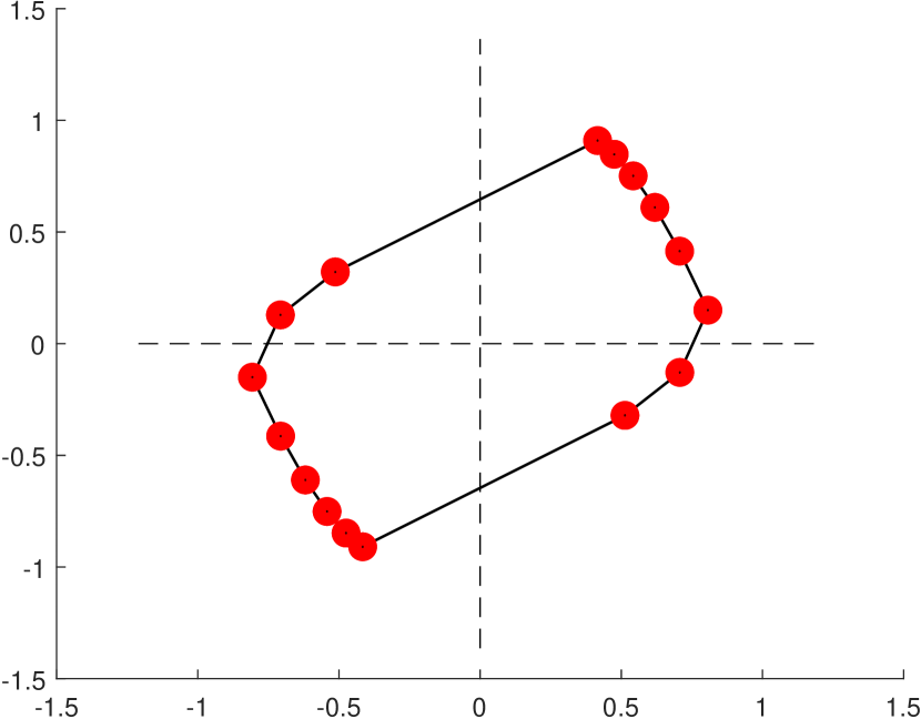
  $L_{1}$

  

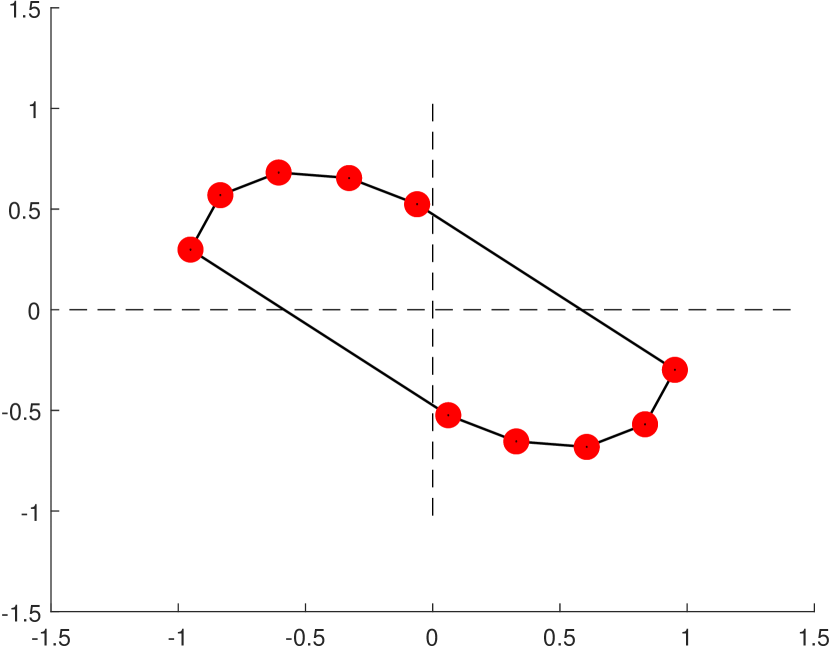
  $L_{2}$

  Figure 5: The polytope extremal multinorm for Example 5.2 with $\tau=2/5$

• Let us fix $\tau=1/10$. We consider the approach with $4$ matrices in Figure 3. We let $\tilde{B}_{1}=e^{\tau B_{1}}$, $\tilde{B}_{2}=e^{\tau B_{2}}$, $A_{1}=e^{\alpha_{1}B_{1}}$ and $A_{2}=e^{\alpha_{2}B_{2}}$.

  We discover that the following is a spectrum maximizing product,

  $$P=\tilde{B}_{1}^{21}\,A_{1}\,A_{2}$$

  which identifies the extremal (constrained) periodic signal

  $$(111111111111111111111111112222222222)^{k}$$

  where every value is taken on an interval of length $1/10$ (see Figure 7).

  We have $\rho=\rho(P)^{5/36}=1.392866831588511$, which gives a lower bound for the Lyapunov exponent:

  (33) $$\sigma\geq 0.331364091942514=\beta(\tau),$$

  improving (31).

  The polytope algorithm takes $18$ iterations to converge and produces the multinorm in Figure 6.

  Applying Algorithm 2 we obtain that the extremal polytope is invariant for the shifted vector field $B_{1,2}-(\beta(\tau)+0.279\ldots){\rm Id}$, from which we get the upper bound

  (34) $$\sigma\leq 0.610\ldots$$

  which also improves (32).

  

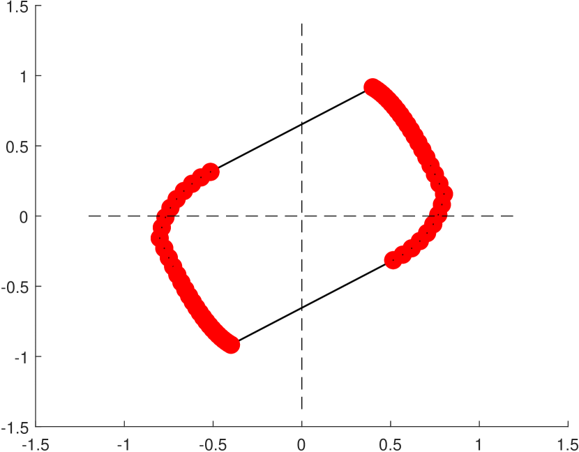
  $L_{1}$

  

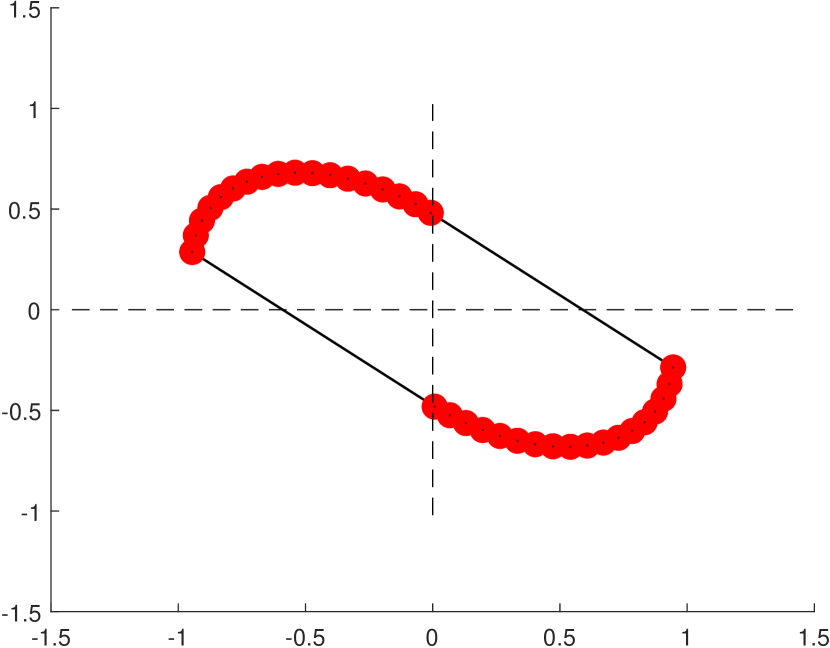
  $L_{2}$

  Figure 6: The polytope extremal multinorm for Example 5.2 with $\tau=1/10$

  

  

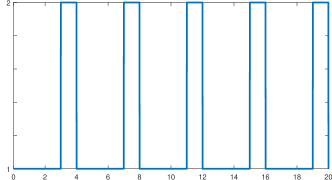
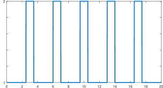
  Figure 7: Optimal signals computed for $\tau=1$ (left) and $\tau=1/2$ and $\tau=2/5$ (right). They both respect dwell times constraints; the signal on the right corresponds to a higher rate of growth.

Example 5.3 (Three matrices).

Let us consider ${{\cal{B}}}=\{B_{1},B_{2},B_{3}\}$ with dwell times given by $\alpha_{1}$, $\alpha_{2}$ and $\alpha_{3}$. We let $\tilde{B}_{1}=e^{\tau B_{1}}$, $\tilde{B}_{2}=e^{\tau B_{2}}$, $\tilde{B}_{3}=e^{\tau B_{3}}$, $A_{1}=e^{\alpha_{1}B_{1}}$ and $A_{2}=e^{\alpha_{2}B_{2}}$, $A_{3}=e^{\alpha_{3}B_{3}}$. The general picture is illustrated by Figure 4.

Appendix

Lemma 5.4.

Let $f:\mathbb{N}\to\mathbb{R}$ be such that for every $j,k\in\mathbb{N}$, $j+k>0$, there exists $\nu_{j,k}\in[0,1]$ such that $f(j+k)\leq\nu_{j,k}f(j)+(1-\nu_{j,k})f(k)$ and $\nu_{j,k}\leq c\frac{j}{j+k}$ with $c$ independent of $j$ and $k$. Then $\lim_{k\to\infty}f(k)$ exists and is equal to $\inf_{k\in\mathbb{N}}f(k)$.

Proof 5.5.

The argument follows the classical proof for sub-additive functions.

Set $f_{\min}:=\inf_{k\in\mathbb{N}}f(k)$ and consider an arbitrary real number $A>f_{\min}$. Fix a positive integer $m$ such that $f(m)<A$. Performing the Euclidean division of every integer $n\geq m$ by $m$ allows one to write $n=qm+r$ with $q\geq 1$ and $0\leq r<m$. Using the hypothesis on $f$, one has that there exists $\nu_{r,qm}\in[0,1]$ such that

$$f(n)\leq\nu_{r,qm}f(r)+(1-\nu_{r,qm})f(qm),$$

and $\nu_{r,qm}\leq c\frac{r}{n}$. A trivial induction on $q\geq 1$ yields that $f(qm)\leq f(m)$. Setting $F(m)=\max_{0\leq r<m}f(r)$, we deduce that for every $n\geq m$, one has that

(35) $$f(n)\leq c\frac{m}{n}F(m)+f(m),\quad\forall n\geq m.$$

Letting $n$ tend to infinity, we get that $\limsup_{n\to\infty}f(n)<A$. The conclusion follows letting $A$ tend to $f_{\min}$.

Acknowledgments

The second author (NG) acknowledges financial support from Italian INdAM - GNCS (Istituto Nazionale di Alta Matematica - Gruppo Nazionale di Calcolo Scientifico).

The work of the fourth author (VP) was prepared within the framework of the HSE University Basic Research Program and funded by the Russian Academic Excellence Project ‘5-100’. Scientific results of Sections 3 and 4 of this paper were obtained with support of RSF Grant 17-11-01027.

References

- [1] C. Basso. Switch-Mode Power Supplies Spice Simulations and Practical Designs. McGraw-Hill, Inc., New York, NY, USA, 1 edition, 2008.
- [2] J. Ben Rejeb, I.-C. Morărescu, A. Girard, and J. Daafouz. Stability analysis of singularly perturbed switched linear systems. In Control subject to computational and communication constraints, volume 475 of Lect. Notes Control Inf. Sci., pages 47–61. Springer, Cham, 2018.
- [3] C. Briat and A. Seuret. Affine characterizations of minimal and mode-dependent dwell-times for uncertain linear switched systems. IEEE Trans. Automat. Control, 58(5):1304–1310, 2013.
- [4] G. Chesi and P. Colaneri. Homogeneous rational Lyapunov functions for performance analysis of switched systems with arbitrary switching and dwell time constraints. IEEE Trans. Automat. Control, 62(10):5124–5137, 2017.
- [5] G. Chesi, P. Colaneri, J. C. Geromel, R. Middleton, and R. Shorten. A nonconservative LMI condition for stability of switched systems with guaranteed dwell time. IEEE Trans. Automat. Control, 57(5):1297–1302, 2012.
- [6] Y. Chitour, P. Mason, and M. Sigalotti. A characterization of switched linear control systems with finite -gain. IEEE Trans. Automat. Control, 62(4):1825–1837, 2017.
- [7] A. Cicone, N. Guglielmi, and V. Y. Protasov. Linear switched dynamical systems on graphs. Nonlinear Anal. Hybrid Syst., 29:165–186, 2018.
- [8] X. Dai. Robust periodic stability implies uniform exponential stability of Markovian jump linear systems and random linear ordinary differential equations. J. Franklin Inst., 351(5):2910–2937, 2014.
- [9] J. C. Geromel and P. Colaneri. Stability and stabilization of continuous-time switched linear systems. SIAM J. Control Optim., 45(5):1915–1930, 2006.
- [10] R. Goebel, R. G. Sanfelice, and A. R. Teel. Hybrid dynamical systems. Princeton University Press, Princeton, NJ, 2012. Modeling, stability, and robustness.
- [11] G. Gripenberg. Computing the joint spectral radius. Linear Algebra Appl., 234:43–60, 1996.
- [12] N. Guglielmi, L. Laglia, and V. Protasov. Polytope Lyapunov functions for stable and for stabilizable LSS. Found. Comput. Math., 17(2):567–623, 2017.
- [13] N. Guglielmi and V. Protasov. Exact computation of joint spectral characteristics of linear operators. Found. Comput. Math., 13(1):37–97, 2013.
- [14] N. Guglielmi and V. Protasov. Invariant polytopes of linear operators with applications to regularity of wavelets and of subdivisions. SIAM J. Matrix Anal. Appl., 37(1):18–52, 2016.
- [15] N. Guglielmi, F. Wirth, and M. Zennaro. Complex polytope extremality results for families of matrices. SIAM J. Matrix Anal. Appl., 27(3):721–743, 2005.
- [16] J. Hespanha and S. Morse. Stability of switched systems with average dwell-time. In Proceedings of the 38th IEEE Conference on Decision and Control, 1999.
- [17] B. Ingalls, E. Sontag, and Y. Wang. An infinite-time relaxation theorem for differential inclusions. Proceedings of the American Mathematical Society, 131(2):487–499, 2003.
- [18] R. Jungers. The joint spectral radius, volume 385 of Lecture Notes in Control and Information Sciences. Springer-Verlag, Berlin, 2009.
- [19] V. Kozyakin. The Berger-Wang formula for the Markovian joint spectral radius. Linear Algebra Appl., 448:315–328, 2014.
- [20] T. Kröger. On-Line Trajectory Generation in Robotic Systems: Basic Concepts for Instantaneous Reactions to Unforeseen (Sensor) Events. Springer Berlin Heidelberg, Berlin, Heidelberg, 1 edition, 2010.
- [21] D. Liberzon. Switching in systems and control. Systems & Control: Foundations & Applications. Birkhäuser Boston, Inc., Boston, MA, 2003.
- [22] D. Liberzon and A. S. Morse. Basic problems in stability and design of switched systems. IIEEE Control Systems Magazine, 19:59–70, 1999.
- [23] T. Mejstrik. Improved invariant polytope algorithm and applications. preprint arXiv:1812.03080.
- [24] A. P. Molchanov and E. S. Pyatnitskiĭ. Lyapunov functions that define necessary and sufficient conditions for absolute stability of nonlinear nonstationary control systems. III. Avtomat. i Telemekh., (5):38–49, 1986.
- [25] A. P. Molchanov and Y. S. Pyatnitskiy. Criteria of asymptotic stability of differential and difference inclusions encountered in control theory. Systems Control Lett., 13(1):59–64, 1989.
- [26] A. S. Morse. Supervisory control of families of linear set-point controllers. I. Exact matching. IEEE Trans. Automat. Control, 41(10):1413–1431, 1996.
- [27] M. Philippe, R. Essick, G. E. Dullerud, and R. M. Jungers. Stability of discrete-time switching systems with constrained switching sequences. Automatica J. IFAC, 72:242–250, 2016.
- [28] M. Philippe, G. Millerioux, and R. M. Jungers. Deciding the boundedness and dead-beat stability of constrained switching systems. Nonlinear Anal. Hybrid Syst., 23:287–299, 2017.
- [29] M. Souza, A. Fioravanti, and R. Shorten. Dwell-time control of continuous-time switched linear systems. In Proceedings of the 54th IEEE Conference on Decision and Control, pages 4661–4666, 2015.
- [30] F. Z. Taousser, M. Defoort, and M. Djemai. Stability analysis of a class of switched linear systems on non-uniform time domains. Systems Control Lett., 74:24–31, 2014.
- [31] A. van der Schaft and H. Schumacher. An introduction to hybrid dynamical systems, volume 251 of Lecture Notes in Control and Information Sciences. Springer-Verlag London, Ltd., London, 2000.
- [32] Y. Wang, N. Roohi, G. Dullerud, and M. Viswanathan. Stability of linear autonomous systems under regular switching sequences. In Proceedings of the 54th IEEE Conference on Decision and Control, pages 5445–5450, 2015.
- [33] W. Xiang. On equivalence of two stability criteria for continuous-time switched systems with dwell time constraint. Automatica J. IFAC, 54:36–40, 2015.
- [34] W. Xiang. Necessary and sufficient condition for stability of switched uncertain linear systems under dwell-time constraint. IEEE Trans. Automat. Control, 61(11):3619–3624, 2016.
- [35] H. Xu, K. L. Teo, and W. Gui. Necessary and sufficient conditions for stability of impulsive switched linear systems. Discrete Contin. Dyn. Syst. Ser. B, 16(4):1185–1195, 2011.