Assessing Practitioner Beliefs about Software Defect Prediction

Abstract.

Just because software developers say they believe in “X”, that does not necessarily mean that “X” is true. As shown here, there exist numerous beliefs listed in the recent Software Engineering literature which are only supported by small portions of the available data. Hence we ask what is the source of this disconnect between beliefs and evidence?.

To answer this question we look for evidence for ten beliefs within 300,000+ changes seen in dozens of open-source projects. Some of those beliefs had strong support across all the projects; specifically, “A commit that involves more added and removed lines is more bug-prone” and “Files with fewer lines contributed by their owners (who contribute most changes) are bug-prone”.

Most of the widely-held beliefs studied are only sporadically supported in the data; i.e. large effects can appear in project data and then disappear in subsequent releases. Such sporadic support explains why developers believe things that were relevant to their prior work, but not necessarily their current work.

Our conclusion will be that we need to change the nature of the debate with Software Engineering. Specifically, while it is important to report the effects that hold right now, it is also important to report on what effects change over time.

1. Introduction

Just because software developers say they believe in “X”, that does not necessarily mean that “X” is true. Jørgensen & Gruschke (Jørgensen and Gruschke, 2009) note that in Software Engineering (SE) domain, seldom lessons from past projects are used to improve future reasoning (to the detriment of new projects). Passos et al. note that developers often assume that lessons learned from a few past projects are general to all future projects (Passos et al., 2011). Devanbu et al. record opinions about software development from 564 Microsoft software developers from around the world (Devanbu et al., 2016). They comment that programmer beliefs can (a) vary with each project and (b) may not necessarily correspond with actual evidence in their current projects. Menzies and Nagappan et al. offer specific examples of this effect. Nagappan et al. (Nagappan et al., 2015) have shown that the much-feared goto statement is usually benign, and sometimes even useful. Menzies et al. recently found no evidence for the delayed issue effect (Menzies et al., 2017) (“The longer a bug remains in the system, the exponentially more costly it becomes to fix”) in 171 industry projects. That study shows that a widely held belief by both practitioners and academics cannot be assumed to always hold.

Table 1. Practitioners’ agreement % on defect prediction metrics (beliefs) reported in a recent IEEE Transactions on Software Engineering (TSE) paper by Wan et al. (Wan et al., 2018).

#	Belief	%
B1	A file with a complex code change process tends to be buggy.	76
B2	A file that is changed by more developers is more bug-prone.	64
B3	A file with more added lines is more bug-prone.	61
B4	Recently changed files tend to be buggy.	58
B5	A commit that involves more added and removed lines is more bug-prone.	57
B6	Recently bug-fixed files tend to be buggy	49
B7	A file with more fixed bugs tends to be more bugprone.	48
B8	A file with more commits is more bug-prone.	46
B9	A file with more removed lines is more bug-prone.	35
B10	Files with fewer lines contributed by their owners (who contribute most changes) are bug-prone.	30

Accordingly, we think it is important to always carefully evaluate developer beliefs. For example, Table 1 lists ten beliefs and software defects listed in a recent TSE’18 paper by Wan et al. (Wan et al., 2018). That study collected 395 responses from practitioners to document developer beliefs about willingness to adopt technologies, challenges, defect prediction metrics, etc. This paper looks for evidence for the Table 1 beliefs in 300,000+ changes seen in dozens of open-source projects. What we find is:

• Two of these beliefs are supported in the data; specifically, “A commit that involves more added and removed lines is more bug-prone” and “Files with fewer lines contributed by their owners (who contribute most changes) are bug-prone”.

• Some of the beliefs supported by the data are not usually endorsed by developers. The last column of Table 1 shows the percent of the 395 developers who endorsed each belief. Note that the last belief (B10) is only endorsed by 30% of the surveyed developers. Yet in our data, it is one of the strongest effects.

• As to the other eight items listed in Table 1, while these have sporadic support in different releases of the same project, there is little overall evidence for these beliefs.

Our conclusion will be that we need to change the nature of the debate with SE. While it is important to report the effects that hold right now, it is also important to report on what effects change over time.

This paper reports strongly supported beliefs and discusses prevalence of beliefs. To make that argument we will use the list of developer beliefs about defect prediction in Table 1. Using that list, we will ask:

• RQ1 : What beliefs are strongly supported in the data? [couleur=gray!10,arrondi=0.1,logo=,ombre=true] Result: We found that beliefs labeled B10 & B5 in  Table 1, which is believed by (30% & 57%) of practitioners has strong support (i.e., large correlations), whereas the more popular belief B1, which is believed by 76% of practitioners, has relatively weaker support.

And to identify the source of disconnect between beliefs and evidence, next we ask:

• RQ2 : Does the same evidence appear everywhere?

  • Do projects show evidence for all the beliefs?

  • Does the size of a release affect belief support?

  • Do beliefs evolve as a project matures (more releases)?

  [couleur=gray!10,arrondi=0.1,logo=,ombre=true] Result: No, the same evidence does not appear everywhere. Only 24% of the projects show support for all the 10 beliefs. And those projects showed support for beliefs among 10% - 36% of their releases. Beliefs appear stronger in smaller than larger releases, with fluctuations like B4 (weaker in large releases but stronger in small releases). Support for beliefs tended to decay than strengthen as the project matured.

The rest of this paper is structured as follows. §2 relates the current work to the prior literature on metrics and instability. In §3, we discuss the choice of our datasets, it’s distribution and brief about our statistical methods we use. §4 details the construction of experiments mapping to literature. Results in §5 and directions to future work in §6. §7 discusses the reliability of our findings. Finally, we summarize and discuss few implications for practice in §8 and §9.

2. Background

2.1. Why Study Practitioner Beliefs?

If we do not understand what factors lead to software defects, then that has detrimental effects for quality assurance, trust, insight, training, and tool development.

• Quality assurance: If we do not know what causes defects in a project, we cannot prevent those problems.

• Training: Another concern is what do we train novice software engineers or newcomers to a project? If our models are not stable, then it is hard to teach what factors most influence software quality.

• Tool development: Further to the last point— if we are unsure what factors most influence quality, it is difficult to design, implement and deploy tools that can successfully improve that quality (e.g. Static analysis tools).

A premise of much research (Lo et al., 2015; Xia et al., 2017, 2019; Zou et al., 2018; Wan et al., 2018) is that knowledge of what factors influence software quality can be discovered by asking software practitioners. But based on the results of this paper, we would say that:

• While such surveys produce a long list of possible effects,

• Only some of which might be relevant to a particular project at a particular time.

2.2. Related Work

Perhaps the closest work to our work is the work by McIntosh & Kamei who, in 2017, reported that the effect on defects of code change properties based on size, entropy, history, and code ownership changes as software systems evolve (McIntosh and Kamei, 2017). Further, they report that although size-related metrics (B3:Added lines & B9:Removed lines) were their top contributors over other metrics, that effect tended to fluctuate across time (and the strength of that effect was project-specific).

To start the research of this paper, we found five papers (Lo et al., 2015; Xia et al., 2017, 2019; Zou et al., 2018; Wan et al., 2018) which list practitioner beliefs, but do not test those beliefs with respect to empirical evidence. From this, we chose a recent qualitative study from IEEE TSE (see Table 1) paper by Wan et al.  (Wan et al., 2018). This paper performed a comprehensive study by gathering practitioners’ opinions (395 responses) on various defect prediction research hypotheses discussed in the literature between 2012-2017. More importantly, they highlight practitioners’ agreement % on defect prediction metrics, prioritization strategy, etc. In support of that work, we work that many of the beliefs reported in (Wan et al., 2018) by Wan et al. were also reported previously in  (D’Ambros et al., 2010; Kamei et al., 2012). In this paper, we revisit these beliefs independently to look for current evidence and reasoning disconnect between beliefs and evidence using the prevalence of their support.

3. Methodology Overview

In this section, we elucidate source, distribution and various attributes we collect from our sample projects. Then we detail the underlying statistical techniques we use to assess our beliefs.

3.1. Data Source & Cleaning

For this work, we wanted to study conclusion instability using a much more detailed approach than the Related Work mentioned above. We analyze 3 times more changes (commits) than recent defect prediction work  (McIntosh and Kamei, 2017; Hoang et al., 2019) and the volume of our dataset is 8 times larger as we expand those changes (commits) that results in 301,627 source code file entries filtered from 524,851 in total.

Turning then to Github, we chose 50 GitHub repository links from a recent defect prediction paper (Walkinshaw and Minku, 2018) that uses Munaiah et al. GitHub project database  (Munaiah et al., 2017). Their work simplified choosing substantive Open Source (OS) samples from GitHub attributing to several metrics such as maturity, active developers, license, etc., We mined file-level commit histories and release information using GitHub API. To minimize bias in our modelling we applied the following sanity checks and discarded projects that have less than,

• 1000 commits

• 10% Bug Fixes

• 5 releases

• 30 developers

• 3 years of activity

And this resulted in 37 projects shown in  Table 2. Our selected projects use many current languages such as Python, Ruby, Java, JavaScript, PHP, etc. To remove noise we ignore test cases, configuration files and static resources such as text, readme, images, etc. To achieve this first we identified source code extensions from our samples they are py, java, rb, c, cpp, h, php, sh, cs, scss, html, scala, js, css, clj, ctp, erb, go, haml, hs and sql . Essentially we consider only the file paths the ends with these extensions, with an additional check that the file/path names do not contain “test”, to eliminate test cases.

Table 2. 37 OS projects developed in popular programming languages. Some projects are developed using multiple programming languages. (Rb - Ruby, Py - Python , JS - JavaScript and SCSS - Sassy-CSS)

URL (github.com/)	Language	URL (github.com/)	Language
activemerchant/active_merchant	Rb	xetorthio/jedis	Java,HTML
activeadmin/activeadmin	Rb,SCSS	spotify/luigi	Py,JS
puppetlabs/beaker	Rb,Shell	lra/mackup	Py
boto/boto3	Py	mikel/mail	Rb
thoughtbot/bourbon	SCSS,HTML	Seldaek/monolog	PHP
bundler/bundler	Rb,HTML	omniauth/omniauth	Rb,HTML
teamcapybara/capybara	Rb	aws/opsworks-cookbooks	Rb
Codeception/Codeception	PHP,HTML	thoughtbot/paperclip	Rb
ooici/coi-services	Py,C/C++	getpelican/pelican	HTML,Py
pentaho/data-access	Java,JS	cakephp/phinx	PHP
pennersr/django-allauth	Py,HTML	propelorm/Propel2	PHP,HTML
encode/django-rest-framework	Py,HTML	puppetlabs/puppetlabs-apache	Rb
django-tastypie/django-tastypie	Py	sferik/rails_admin	JS,Rb
doorkeeper-gem/doorkeeper	Rb	reactjs/react-rails	JS,Rb
drapergem/draper	Rb,HTML	resque/resque	Rb
errbit/errbit	Rb,HTML	restsharp/RestSharp	C#
jordansissel/fpm	Rb	mperham/sidekiq	Rb,JS
ros-simulation/gazebo_ros_pkgs	C&C++	plataformatec/simple_form	Rb
ruby-grape/grape	Rb,HTML

3.2. Data distribution

Overall this sample contains data modified in the period 2005 to 2019 by 12,361 developers in over 524,000 file entries. These modifications were made to 127,950 active branch commits (in all, 19,617,483 line insertions and 13,642,341 line deletions). On average our chosen set of projects has been active for over 7 years (see the distributions of Figure 1). The OS projects we chose for this study are publicly available. All our data is on-line so that other researchers can benefit (see github.com/ai-se/defect_perceptions).

3.3. Data Attributes

We mine the entire commit history of a project. A tuple of our main dataset contains the following attributes unique commit_id, commit_time, the author who pushed the changes commit_author, affected file_path, number of lines inserted and deleted (insertions, deletions). Importantly for every commit, we set a label Bug Fixing Commit (BFC) as 1, if it was pushed in an attempt to fix bug (s) or 0 if otherwise. We achieve this by scanning the commit message, if they contained any derivatives of the following stemmed words like bug, fix, issu, error, correct, proper, deprecat, broke, optimize, patch, solve, slow, obsolete, vulnerab, debug, perf, memory, minor, wart, better, complex, break, investigat, compile, defect, inconsist, crash, problem or resol. We also identify releases of each project using Git releases/tags.

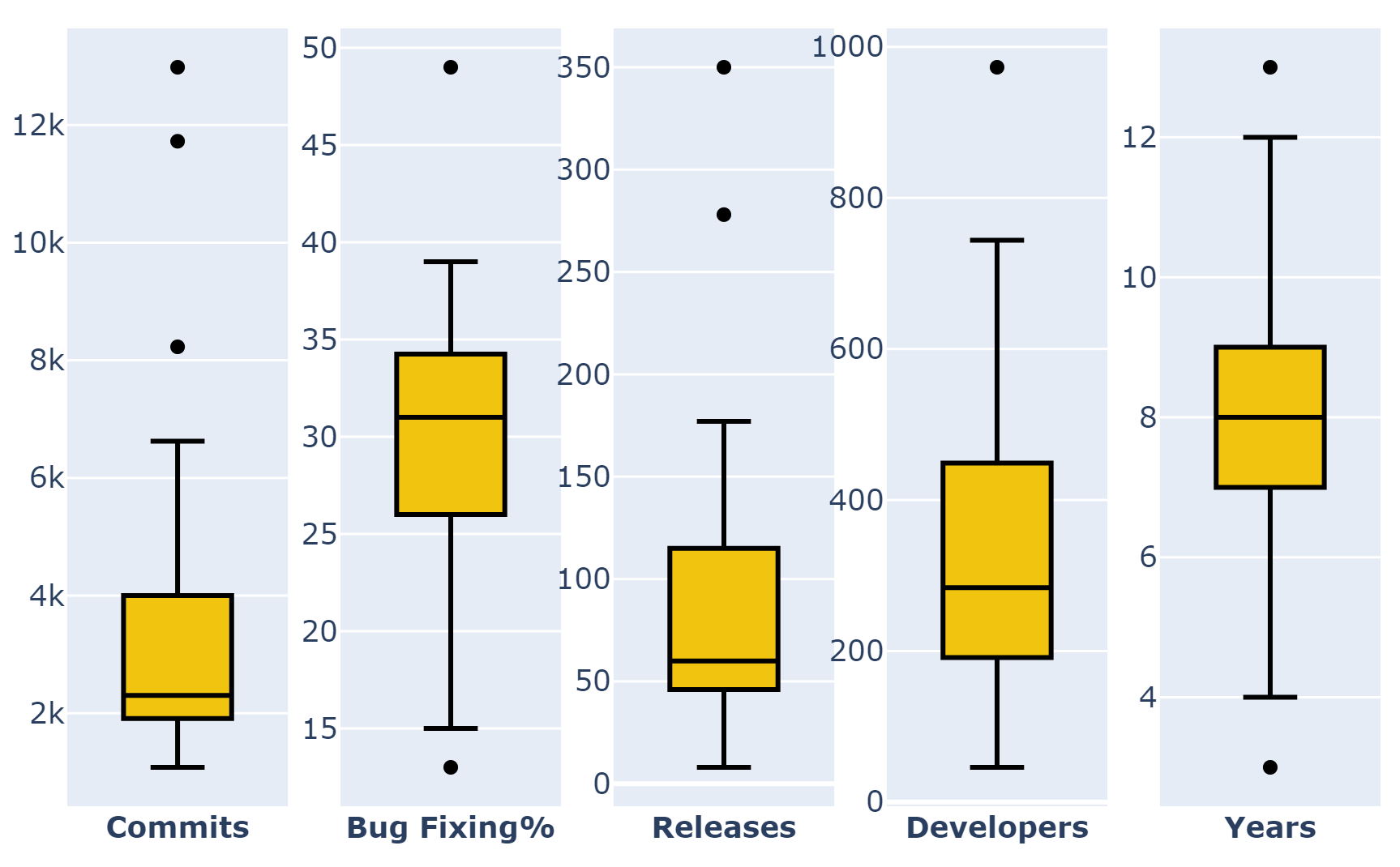
Figure 1. Distribution of Commits (2304), Bug Fixing (31%) Releases (60), Developers (284) and Years (8) active among 37 projects. $\tilde{x}$ (median)

3.4. Method

Our work requires us to measure the following two items:

• Effect: Significant associations between beliefs and defect proneness.

• Rank: Significant differences among these associations.

3.4.1. Effect:

We use Spearman’s rank correlation (a non-parametric test) to assess associations between independent variable “$F_{BX}$” and dependent variable“$F_{D}$” (detailed in §4). We chose Spearman like a previous defect prediction study  (D’Ambros et al., 2010) recommended to handle skewed data, further it is unaffected by transformations (log, square-root etc) on variables.

The Spearman’s rank correlation, $\rho=\frac{\text{cov}(X,Y)}{\sigma_{x}\sigma_{y}}$ between two samples $X,Y$ (with means $\overline{x}$ and $\overline{y}$), as estimated using $x_{i}\in X$ and $y_{i}\in Y$ via

$$\rho=\frac{{}\sum_{i=1}^{n}(x_{i}-\overline{x})(y_{i}-\overline{y})}{\sqrt{\sum_{i=1}^{n}(x_{i}-\overline{x})^{2}(y_{i}-\overline{y})^{2}}}$$

We conclude using both correlation coefficient ($\rho$) and its associated p_value in all our experiments. $\rho$ varies from 1, i.e., ranks are identical, to $-1$, i.e., ranks are the opposite, where 0 indicates no correlation.

• Higher $\rho$ value indicates more evidence for defect prone.

• Lower $p\_value$ indicates significant result.

3.4.2. Rank:

Populations may have the same median while their distribution could be very different. Hence to identify significant differences or rank among two or more populations we use Scott-Knott test recommended by Mittas et al. in TSE’13 paper (Mittas and Angelis, 2013). Scott-Knott is a top-down bi-clustering approach used to rank different treatments, the treatment could be beliefs, project, release or any conjunction. This method sorts a list of $l$ treatments with $\mathit{ls}$ measurements by their median score. It then splits $l$ into sub-lists m, n in order to maximize the expected value of differences in the observed performances before and after divisions.

For lists $l,m,n$ of size $\mathit{ls},\mathit{ms},\mathit{ns}$ where $l=m\cup n$, the “best” division maximizes $E(\Delta)$; i.e. the difference in the expected mean value before and after the spit:

$$E(\Delta)=\frac{ms}{ls}abs(m.\mu-l.\mu)^{2}+\frac{ns}{ls}abs(n.\mu-l.\mu)^{2}$$

Further, to avoid “small effects” with statistically significant results we employ the conjunction of bootstrapping and A12 effect size test by Vargha and Delaney  (Vargha and Delaney, 2000) for the hypothesis test H to check if m, n are truly significantly different. These techniques do not make gaussian assumptions (non-parametric).

3.5. Terminologies

In this section, we briefly introduce common labels, definitions, and thresholds that we weave while discussing the results.

We label beliefs as,

• popular if they have more than 50% agreement in Table 1

• unpopular otherwise.

3.5.1. Evidence:

We use Spearman’s rank correlation (detailed in §3) $\rho$ ranges shown below to discuss strength of the evidence. From the usage of Spearman’s $\rho$ in this defect prediction literature  (Zimmermann et al., 2007) we derive the following ranges for $|\rho|$ :

While these ranges are debatable, we note that the results shown below are of such a “large effect size” that the details of these thresholds do not threaten the validity of our conclusion. But importantly these ranges have lesser impact on our conclusion as we are keen on relative ranks obtained from Scott-Knott-test of §3.4.2 deduced from overall population of $\rho$ scores.

3.5.2. Project Support Population ($P_{BX}$)

$P_{BX}$ is the population of significant $\rho$ scores computed for a belief $BX$ beliefs 1 to 10 ie, $X\in[1..10]$ for all releases $R$ in project $P$, Thus,

$$P_{BX}=\{\rho(\{F_{BX}\},\{F_{D}\})\}$$

To recollect, $\rho$ is the association between:

• $F_{BX}$, which is the metric we collect from the Github data

• and $F_{D}$ which is the defects fixed during 6 months after the release $r$ (i.e. the defects that anyone thought were worth acting on).

We only consider significant (99% confidence level) $\rho$ scores. This implies that some releases are not considered in the population.

In the following, $|P_{BX}|$ is the number of releases in the project $P$, such that $|P_{BX}|\leq R$. where $R$ is the total number of releases in a project $P$.

4. Assessing Beliefs

In this section, we describe the construction of our correlation experiments using the underlying rationale and relevant literature attached to each of the beliefs in  Table 1. Then, we discuss the role of relevant attributes scraped from our sample projects to be used as an independent variable to compute associations.

[couleur=gray!10,arrondi=0.1,logo=,ombre=true] Objective: To export $P_{BX}$ which is a population of significant $\rho$ scores for a belief $BX$, where each score is computed as a correlation between, $F_{BX}\&F_{D}$ and collected over all releases $R$ in a project $P$. This is repeated for all 37 projects and 10 beliefs.

To support this objective:

• $r:$ is a release in project $p$. We ignore first release of all projects $r>1$.

• $F:$ is a file created or modified during the pre-release $r$ period.

• $BX:$ denotes metric associated with beliefs 1 to 10, $X\in[1..10]$.

• $F_{BX}:$ denotes metric captured on file $F$

• $D:$ defects fixed 6 months after $r$ (post-release bugs)

• $F_{D}:$ defects fixed 6 months after $r$ (post-release bugs) on $F$

We employ the traditional release based approach to assess our beliefs. We capture metrics in the pre-release period to find associations with post-release bugs 6 months after the release. We assess the beliefs “$BX$” for all releases in a project. We then build a population with the effect scores collected in all releases and projects to be analyzed in the §5. In each release, we compute the belief metric for each distinct file “$F$” modified in a release $r$ where $r\in R$ (total number of releases). And defect proneness “$D$” is the number of post-release bugs. Then “$F_{D}$” is the number of post-release ($r+6$months) bugs on file “$F$”. Hence, “$F_{D}$” computation is common across all the beliefs whereas “$F_{BX}$” (belief metric on a file) captured during the pre-release period $r$ is elucidated in the following sections.

In the following, we discuss the specifics of how to assess the beliefs of Table 1.

4.1. B1: Complex Code Changes

Description: “A file with a complex code change process tends to be buggy”. In 2009, Hassan (Hassan, 2009) adopted Shannon Entropy from information theory to devise few code change models that weigh scattered modifications (complexity) of a file using its change history. The intuition behind this belief is that change scattering of a file over some periods makes it cumbersome for developers to maintain, thus making it defect prone. We use Hassan’s compute History Complexity Metric ($HCM^{1d}$) with the decay factor ($d$) to assess this belief. The decay factor is used to undermine earlier modifications.

Procedure: We divide the pre-release period $r$ into bi-weekly (14 days) periods to compute entropy $HCM$ for a file $F$ and this will be $F_{B1}$. In cases where releases have less than 14 days, $r$ will have just two equal size periods. We then export the correlation between $F_{B1}$ & $F_{D}$.

4.2. B2 & B10: Ownership

Description: B2:“Files changed by more developers are more buggy”. In 2010, Matsumoto et al.  (Matsumoto et al., 2010) showed human factors can be used to forecast defects. Specifically, they saw that files touched by more developers make the file prone to defects.

B10:“Files with fewer lines contributed by their owners (who contribute most changes) are bug-prone”. Bird et al. in their work  (Bird et al., 2011) explore various ownership related metrics. We employ their idea of minor & major contributor, where many minor contributors modifying a file makes it defect prone. They define a minor contributor as someone who has made less than 5% changes and a major contributor as someone who has made at-least 5% or more. Thus if a file in a release has changed by a large proportion of minor contributors it is prone to more defects.

Procedure: $F_{B2}$ here is the count of distinct commit authors who made some change to the file in the pre-release. $F_{B10}$ is the % of minor contributors (who contributed less than 5% code churn) for file $F$ in the pre-release. We then export the correlation between $F_{B2}$ & $F_{D}$ and $F_{B10}$ & $F_{D}$.

4.3. B3 & B9 : Code Churn

Description: B3:“A file with more added lines is more bug-prone” and B9:“A file with more removed lines is more bug-prone”. In 2005 Nagappan & Ball in  (Nagappan and Ball, 2005) showed that relative code churns of files using number of added or deleted lines between subsequent versions are good indicators to forecast defects.

Procedure: We measure $F_{B3}$ or $F_{B9}$ for a file $F$ by aggregating on the number of lines added (B3) or number of lines deleted (B9) only during the pre-release period $r$. We then export the correlation between $F_{B3}$ & $F_{D}$ and $F_{B9}$ & $F_{D}$.

4.4. B4 & B6: Temporal

Description: Two of these temporal heuristics are introduced and explored by Hassan et al. (Hassan and Holt, 2005) in their popular work, “Top 10 list for dynamic defect prediction”. B4:“Recently changed files tend to be buggy” and B6:“Recently bug-fixed files tend to be buggy”. The rationale here is that files modified closer to release periods may not be tested effectively and as a result, recently changed files would tend to introduce more bugs (also see  (Graves et al., 2000)) in the near future (B4). Another intuition is that faults tend to arise at the same spot is a good indicator to measure defect proneness (B6).

Procedure: Attributes commit_time (longer value indicates more recent) and BFC (1 indicates bug fixing, 0 otherwise) are used to model these two beliefs. But a file can be modified (committed) multiple times in the pre-release period. Hence, we assign the maximum commit_time for $F_{B4}$, similarly we assign the maximum commit_time for $F_{B6}$; provided BFC = 1 in the pre-release period. Further in $F_{B6}$ if a file is never modified for the purpose of fixing a defect in the pre-release period, its ignored for analysis. We then export the correlation between $F_{B4}$ & $F_{D}$ and $F_{B6}$ & $F_{D}$.

4.5. B5: Commit Churns

Description: “A commit that involves more added and removed lines is more bug-prone.”. A single commit affects one or more files with some line additions and/or deletions. Hindle et al.  (Hindle et al., 2008) and Hattori et al.  (Hattori and Lanza, 2008) studied the nature and distribution of large commits in terms of the number of files it changed and highlighted that although large commits are rare they are unsafe to ignore. A commit can push the same (or more) amount of line changes with fewer files. Thus rather than the number of files a commit changes, we weigh this belief based on the amount of added and removed lines a commit pushes into the system.

Procedure: Unlike other beliefs, that can be measured at file-level, a commit is a collection of files. It’s immutable, meaning it cannot be directly traced in the post-release period. Hence, we assess the impact of a commit using the files it affected. Thus, the independent variable is a commit in the pre-release period $F_{B5}$ (represents a commit), which is an aggregate of code churn (insertions + deletions) for all the files part of the commit. Similarly, commit defect proneness is the aggregation of file defect proneness $F_{D}$ in the post-release period. In other words, we collectively correlate between a file $F$ that is part of a large commit in the pre-release period with the number of bugs introduced by $F$ in the post-release period. We then export the correlation between $F_{B5}$ & $F_{D}$.

4.6. B7 & B8: Something More

Description: Graves et al. in  (Graves et al., 2000) found an effect among the two process-related metric B7 & B8 ie., “A file with more fixed bugs tends to be more bug-prone” and “A file with more commits is more bug-prone” through analyzing code from a telephone switching system.

Procedure: $F_{B7}$ is the count of bug fixes on file $F$ and $F_{B8}$ is the count of modifications (commits) made on file $F$, computed during their corresponding pre-release periods. We then export the correlation between $F_{B7}$ & $F_{D}$ and $F_{B8}$ & $F_{D}$.

5. Results

In this section, we explore two of our RQ’s. For each RQ we discuss the motivation, approach, and findings.

5.1. RQ1: What beliefs are strongly supported in the data?

Motivation: Similar to the work by Devanbu et al. in  (Devanbu et al., 2016) we compare practitioners’ agreement % with empirical evidence. Our objective here is to find beliefs that have strong support.

Approach: We compute $P_{BX}$ for each belief $BX$ for all the 37 projects. This results in 10 independent $P_{BX}$ populations one for each belief. Next, we rank these populations by their median and effect difference using the Scott-Knott-test of §3.4.2. That results in Table 3 which we compare with practitioners’ agreement % in  Table 1.

Table 3. Scott-Knott test applied to all the 10 beliefs, that contains support $\rho$ scores of 3,198 releases in all the 37 projects. Each row represents a population of $P_{BX}$ scores across all 37 projects. (Higher rank indicates stronger support). IQR - Interquartile Range.

Rank	Belief	Median	IQR
1	B9 (35%)	43	27
1	B4 (58%)	44	28
2	B3 (61%)	45	21
2	B1 (76%)	46	21
2	B6 (49%)	49	47
2	B7 (48%)	49	22
2	B2 (64%)	50	21
2	B8 (46%)	51	22
3	B10 (30%)	63	23
4	B5 (57%)	71	26

Findings: Using the results in Table 3 we report popular belief B10 and unpopular belief B5 have significantly strong support. Surprisingly, these unpopular beliefs B6,B7,B8 and B10 have better support than some popular beliefs B1, B3 & B4. For example:

• The ownership-based belief B10 with only 30% practitioner agreement shows strong support.

• The temporal belief B4 though with 58% practitioner agreement has relatively weaker support 0.4. B1 with the largest practitioner agreement 76% shows weak support.

Overall, only a few beliefs B2,B5 & B9 are in agreement (%) with practitioners beliefs. Of those, B5:Large Commits, with 57% practitioner agreement has the highest effect (0.7) among all the beliefs.

[couleur=gray!10,arrondi=0.1,logo=,ombre=true] Result: We found that beliefs labeled B10 & B5 in  Table 1, which is believed by (30% & 57%) of practitioners has strong support (i.e., large correlations), whereas the more popular belief B1, which is believed by 76% of practitioners, has relatively weaker support.

5.2. RQ2 : Does the same evidence appear everywhere?

Figure 2. Coverage of beliefs $P_{c}$ and its prevalence among releases $P_{r}$ is shown here. Projects are sorted based on $P_{C}$. $P_{C}$ is the count of beliefs that show at least a minimum support in the project. $P_{r}\%$ is the proportion of aggregated experiments that show at least a minimum support in the project for all the beliefs.

Table 4.

Rank	Treatment	Median	IQR
1	$L_{B9(35\%)}$	33	21
1	$L_{B6(49\%)}$	34	23
1	$L_{B4(58\%)}$	37	22
2	$L_{B1(76\%)}$	38	17
2	$L_{B3(61\%)}$	38	14
2	$L_{B8(46\%)}$	41	19
2	$L_{B2(64\%)}$	42	18
2	$L_{B7(48\%)}$	42	19
3	$L_{B10(30\%)}$	52	22
3	$M_{B9(35\%)}$	52	14
3	$M_{B4(58\%)}$	54	16
3	$M_{B7(48\%)}$	54	14
3	$M_{B3(61\%)}$	54	12
3	$M_{B2(64\%)}$	55	14
3	$M_{B8(46\%)}$	55	13
3	$M_{B1(76\%)}$	55	17
3	$M_{B6(49\%)}$	55	24
4	$L_{B5(57\%)}$	63	25
5	$M_{B10(30\%)}$	65	15
5	$S_{B1(76\%)}$	66	4
5	$M_{B5(57\%)}$	69	23
5	$S_{B2(64\%)}$	74	13
5	$S_{B6(49\%)}$	75	22
5	$S_{B9(35\%)}$	74	15
5	$S_{B3(61\%)}$	76	19
5	$S_{B7(48\%)}$	78	16
6	$S_{B10(30\%)}$	80	15
6	$S_{B4(58\%)}$	82	20
6	$S_{B8(46\%)}$	80	16
6	$S_{B5(57\%)}$	87	18

Motivation: The above results show that, overall, many commonly held beliefs do not always hold across all the data. But this is not to say that sometimes it may be true that some of the beliefs of Table 1 are not true.

Devanbu et al. (Devanbu et al., 2016) found that practitioners had different opinions working for different projects, within the same organization. To explore the source of that disconnect, we wish to investigate irregularities of evidence among projects, releases and over time, thus we ask :

• a) Do projects show evidence for all the beliefs?

• b) Does the size of a release affect belief support?

• c) Do beliefs evolve as a project matures (more releases)?

a) Do projects show evidence for all the beliefs ?

Approach: For each project we measure coverage of beliefs $P_{C}$, which is simply the number of beliefs a project $P$ shows at least a minimum support. In other words a project $P$ covers a belief $BX$ if $\tilde{x}(P_{BX})\geq 0.4$. Then, we measure $P_{r}\%$ (release prevalence) which is the proportion of our aggregated correlation experiments that shows at least a minimum support. To compute this we aggregate $P_{BX}$ for all 10 beliefs for a project $P$. Then using this aggregated population we compute the % of $\rho\geq 0.4$ .

Findings: The results in Figure 2 show that:

• Only 24% of the projects show support for all the 10 beliefs.

• Only 24% of projects show support for less than 5 beliefs (but projects that covered all 10 beliefs had their evidence in only (10 - 36%) of its releases).

b) Does the size of a release affect belief support?

Approach: We define size of a release based on the number of files created or modified in a release. To measure fluctuations, first we group releases into three non-overlapping categories namely small, medium & large based on the number of distinct files $D_{F}$ in a release. Using the distribution of $D_{F}$ among releases of all the 37 projects, we find the $\tilde{x}(D_{F})$ to be 18 (files). And using the Inter-Quartile range of this distribution, we place a release $r$ of a project $P$ in one of the following categories:

• small: If, $3<D_{F}<18$ ($\tilde{x}$)

• medium: If, $18\leq D_{F}<Q3$ (Third quartile)

• large: If, $D_{F}\geq Q3$ (Third quartile)

Then, for each belief $BX$ we segregate the support score population $P_{BX}$ (computed in RQ1) into three different populations based on size of the release. After grouping, this results in 30 populations (treatments) which we cluster using Scott-Knott-test§3.4.2, resulting in Table 4. Note that we group releases based on the number of files $D_{F}$ rather than the median duration (21 days), since we model our experiments based on files $F$. This decision should not affect our experiment as we tested $D_{F}$ and its corresponding release duration to be positively correlated with strong support of 0.6 (median); considering all releases in all the 37 projects.

Findings: We observe a clear drift in effect distribution among the three release sizes in Table 4, indicating size of a release affects belief support. For example, temporal belief B4 shows strong support in small releases but not in large releases. Notably, smaller releases have better support than larger releases. Thus, in summary, Table 4 tells us that we can reason better about smaller releases than larger releases.

That said, it is important to add that while 47% of releases in our projects are small, only 18% (718 releases) of them were qualified for the treatments above as the rest were insignificant ($p\_value\geq 0.01$). So while our conclusions about small releases are a promising result, overall across all our data, it holds for a very small group.

c) Do beliefs evolve as a project matures (more releases)?

Approach: To observe whether belief support tend to strengthen or decay as a project matures with more releases, we test if there is a linear relationship between belief support and its maturity. To measure this, we correlate between all release dates ($\{r_{date}\}$) of a project with its corresponding support scores $P_{BX}$ for a belief $BX$.

The $Growth(\%)$ for a belief is the proportion of projects that shows a correlation $\rho\geq 0.4$ (indicating a positive relationship between release dates and belief support). Similarly, $Decay(\%)$ for a belief is the proportion of projects that shows a correlation $\rho\leq-0.4$ (indicating a negative relationship between release dates and belief support).

Figure 3. Evolution of beliefs among all 37 projects. Growth % is the proportion of projects where a corresponding belief correlated with $\rho\geq 0.4$ between project release dates and empirical evidence ($P_{BX}$). And, Decay % is the proportion of projects where a corresponding belief correlated with $\rho\leq-0.4$ between project release dates and empirical evidence ($P_{BX}$). Beliefs in the plot are sorted based on Decay %.

Findings: Figure 3 show some support for beliefs both decaying and growing. Beliefs B6 & B9 show growth in 21% of the projects. Four of the beliefs (B2, B4, B9 & B10) are decaying in more than 25% of the projects with the highest decay of 51% is observed with ownership-based belief B10 and notably the growth of just 2%.

That said, the major trend in Figure 3 is that beliefs tend to decay, not strengthen as a project matures. Further, we highlight that we only assessed for linearity and we don’t delve into the magnitude of this effect which would remain a future work.

[couleur=gray!10,arrondi=0.1,logo=,ombre=true] Result: No, the same evidence does not appear everywhere. Only 24% of the projects show support for all the 10 beliefs. And those projects showed support for beliefs among 10% - 36% of their releases. Beliefs appear stronger in smaller than larger releases, with fluctuations like B4 (weaker in large releases but stronger in small releases). Support for beliefs tended to decay than strengthen as the project matured.

6. Future directions

We portrayed various irregularities of beliefs in data. Krishna et al. through transfer learning techniques (Krishna et al., 2016; Krishna and Menzies, 2018) showed instabilities can be minimized by identifying a representative oracle project among ‘$N$’ projects. But in our opinion, as a project evolves it is more likely that such an oracle may need frequent adjustments or even replacements. Thus in a result analogous to Menzies et al. in  (Menzies et al., 2011), we advise focusing on factors that help to answer when & where support for beliefs holds for our future work.

Other researchers endorse our call for more reasoning about the context in SE. Recently Zhang et al. in  (Zhang et al., 2014) showed improved global predictive power by including 6 context factors ( i.e., programming language, issue tracking, the total lines of code, the total number of files, the total number of commits, and the total number of developers). Notably only 3 out of 21 defect prediction works cited Petersen & Wohlin’s context factors  (Petersen and Wohlin, 2009) (2009) in the past decade.

7. Threats to validity

7.1. Threats to internal validity

This paper only explored 10 of the 15 metric-related beliefs documented by Wan et al. (Wan et al., 2018) in Table 1. We found that some of the modeling decisions about how to map data into Table 1 required extensive, possibly even arcane, explanations. Objectively, we were able to answer our central question using the 10 beliefs and it would remain the same with or without exploring additional beliefs. Like this prominent (Ray et al., 2014) and a recent  (Walkinshaw and Minku, 2018) large scale analysis, we rely on labeling commit messages for bug fixes as our independent variable. Due to limitations in the heuristics used to generate those labels (Śliwerski et al., 2005; Fan et al., 2019), such labels might be misleading. To partially mitigate this issue of false negatives, we expanded our set of keywords for better coverage, which we detailed in §3. To validate if false positives impacted our results, we cross-checked whether projects with higher Bug Fix % were likely to show support for more beliefs.

7.2. Threats to external validity

Our work is biased by the projects and data found in our sample. This means that our conclusions could differ from other publications. For example, many of those publications discussed C and C++ projects while our sample contained many Ruby projects. Having said this, our sample sufficiently covers many popular programming languages like Python, Java, etc. All our projects are OS but Agrawal et al. in  (Agrawal et al., 2018) showed that many open-source lessons hold for in-house. We identified releases using git tags which mark a boundary for readiness in the commit. Some of these changes were too small (just a few hours) even for rapid releases  (Mäntylä et al., 2015). Hence, we only consider releases that had at least 3 distinct files changed.

7.3. Threats to statistical conclusion validity

Our conclusions are based on correlation which means the strength (or weakness) of this analysis is the same as the strength or weakness of correlation. To increase the validity of those conclusions, we only reported significant at the 0.01 level. Also, we ignored correlations with less than 4 observations even at a significant level. As some releases have less than 3 files changed and technically it is possible to get high correlation with a zero p_value with just two observations, but we considered this unwise (so we deleted such conclusions).

8. Summary

At the start of a software analytics project, it is important to focus software analytics on questions of interest to the client. Therefore, it is very important to document developer beliefs, as done by Wan et al.  (Wan et al., 2018). That being said, once project data becomes available, it is just as important to update the focus in accordance with the observed effects.

In this paper, we report the source of the disconnect between practitioners’ perception of defect prediction metrics and empirical evidence. We argue sporadicity of evidence prevalence is the leading cause of the disconnect between stated beliefs (e.g. the Wan et al.  (Wan et al., 2018) paper) and observed evidence. Despite irregularities, we offer few beliefs that stood out B5 (Large Commits) and B10 (Owner contribution) with good prevalence in our large scale study. Thus we encourage developers to update their beliefs when the evidence demands it. This paper also observed fluctuations of evidence in a new dimension (size of a release).

9. Implications for Practice

Inferring from the results in §5 we say:

• Yes, we should study working software engineers to learn a list of effects that might damage software quality;

• But no, do not assume that all those effects hold at all times over the current project.

More specifically, when setting policies for software projects, managers and project leads should not “bet” on a small number of effects. Rather, they should:

• Perpetually monitor for the presence, or absence of a range of effects (such as those listed in Table 1);

• Perpetually adjust their code review and code refactoring processes such that they learn (a) not to trigger on old effects that now no longer hold or (b) trigger on new effects that have just appeared.

- (1)
- Agrawal et al. (2018) Amritanshu Agrawal, Akond Rahman, Rahul Krishna, Alexander Sobran, and Tim Menzies. 2018. We don’t need another hero?: the impact of heroes on software development. In Proceedings of the 40th International Conference on Software Engineering: Software Engineering in Practice. ACM, 245–253.
- Bird et al. (2011) Christian Bird, Nachiappan Nagappan, Brendan Murphy, Harald Gall, and Premkumar Devanbu. 2011. Don’t touch my code!: examining the effects of ownership on software quality. In Proceedings of the 19th ACM SIGSOFT symposium and the 13th European conference on Foundations of software engineering. ACM, 4–14.
- D’Ambros et al. (2010) Marco D’Ambros, Michele Lanza, and Romain Robbes. 2010. An extensive comparison of bug prediction approaches. In 2010 7th IEEE Working Conference on Mining Software Repositories (MSR 2010). IEEE, 31–41.
- Devanbu et al. (2016) Premkumar Devanbu, Thomas Zimmermann, and Christian Bird. 2016. Belief & evidence in empirical software engineering. In 2016 IEEE/ACM 38th International Conference on Software Engineering (ICSE). IEEE, 108–119.
- Fan et al. (2019) Yuanrui Fan, Xin Xia, Daniel Alencar da Costa, David Lo, Ahmed E Hassan, and Shanping Li. 2019. The Impact of Changes Mislabeled by SZZ on Just-in-Time Defect Prediction. IEEE Transactions on Software Engineering (2019).
- Graves et al. (2000) Todd L Graves, Alan F Karr, James S Marron, and Harvey Siy. 2000. Predicting fault incidence using software change history. IEEE Transactions on software engineering 26, 7 (2000), 653–661.
- Hassan (2009) Ahmed E Hassan. 2009. Predicting faults using the complexity of code changes. In Proceedings of the 31st International Conference on Software Engineering. IEEE Computer Society, 78–88.
- Hassan and Holt (2005) A. E. Hassan and R. C. Holt. 2005. The top ten list: dynamic fault prediction. In 21st IEEE International Conference on Software Maintenance (ICSM’05). 263–272. https://doi.org/10.1109/ICSM.2005.91
- Hattori and Lanza (2008) Lile P Hattori and Michele Lanza. 2008. On the nature of commits. In Proceedings of the 23rd IEEE/ACM International Conference on Automated Software Engineering. IEEE Press, III–63.
- Hindle et al. (2008) Abram Hindle, Daniel M German, and Ric Holt. 2008. What do large commits tell us?: a taxonomical study of large commits. In Proceedings of the 2008 international working conference on Mining software repositories. ACM, 99–108.
- Hoang et al. (2019) Thong Hoang, Hoa Khanh Dam, Yasutaka Kamei, David Lo, and Naoyasu Ubayashi. 2019. DeepJIT: an end-to-end deep learning framework for just-in-time defect prediction. In Proceedings of the 16th International Conference on Mining Software Repositories. IEEE Press, 34–45.
- Jørgensen and Gruschke (2009) Magne Jørgensen and Tanja M. Gruschke. 2009. The Impact of Lessons-Learned Sessions on Effort Estimation and Uncertainty Assessments. Software Engineering, IEEE Transactions on 35, 3 (May-June 2009), 368 –383.
- Kamei et al. (2012) Yasutaka Kamei, Emad Shihab, Bram Adams, Ahmed E Hassan, Audris Mockus, Anand Sinha, and Naoyasu Ubayashi. 2012. A large-scale empirical study of just-in-time quality assurance. IEEE Transactions on Software Engineering 39, 6 (2012), 757–773.
- Krishna and Menzies (2018) Rahul Krishna and Tim Menzies. 2018. Bellwethers: A baseline method for transfer learning. IEEE Transactions on Software Engineering (2018).
- Krishna et al. (2016) Rahul Krishna, Tim Menzies, and Wei Fu. 2016. Too much automation? The bellwether effect and its implications for transfer learning. In Proceedings of the 31st IEEE/ACM International Conference on Automated Software Engineering. ACM, 122–131.
- Lo et al. (2015) David Lo, Nachiappan Nagappan, and Thomas Zimmermann. 2015. How practitioners perceive the relevance of software engineering research. In Proceedings of the 2015 10th Joint Meeting on Foundations of Software Engineering. ACM, 415–425.
- Mäntylä et al. (2015) Mika V Mäntylä, Bram Adams, Foutse Khomh, Emelie Engström, and Kai Petersen. 2015. On rapid releases and software testing: a case study and a semi-systematic literature review. Empirical Software Engineering 20, 5 (2015), 1384–1425.
- Matsumoto et al. (2010) Shinsuke Matsumoto, Yasutaka Kamei, Akito Monden, Ken-ichi Matsumoto, and Masahide Nakamura. 2010. An analysis of developer metrics for fault prediction. In Proceedings of the 6th International Conference on Predictive Models in Software Engineering. ACM, 18.
- McIntosh and Kamei (2017) Shane McIntosh and Yasutaka Kamei. 2017. Are fix-inducing changes a moving target? a longitudinal case study of just-in-time defect prediction. IEEE Transactions on Software Engineering 44, 5 (2017), 412–428.
- Menzies et al. (2011) Tim Menzies, Andrew Butcher, Andrian Marcus, Thomas Zimmermann, and David Cok. 2011. Local vs. global models for effort estimation and defect prediction. In 2011 26th IEEE/ACM International Conference on Automated Software Engineering (ASE 2011). IEEE, 343–351.
- Menzies et al. (2017) Tim Menzies, William Nichols, Forrest Shull, and Lucas Layman. 2017. Are delayed issues harder to resolve? Revisiting cost-to-fix of defects throughout the lifecycle. Empirical Software Engineering 22, 4 (2017), 1903–1935.
- Mittas and Angelis (2013) N. Mittas and L. Angelis. 2013. Ranking and Clustering Software Cost Estimation Models through a Multiple Comparisons Algorithm. IEEE Trans SE 39, 4 (April 2013), 537–551. https://doi.org/10.1109/TSE.2012.45
- Munaiah et al. (2017) Nuthan Munaiah, Steven Kroh, Craig Cabrey, and Meiyappan Nagappan. 2017. Curating GitHub for engineered software projects. Empirical Software Engineering 22, 6 (2017), 3219–3253.
- Nagappan et al. (2015) Meiyappan Nagappan, Romain Robbes, Yasutaka Kamei, Éric Tanter, Shane McIntosh, Audris Mockus, and Ahmed E Hassan. 2015. An empirical study of goto in C code from GitHub repositories. In Proceedings of the 2015 10th Joint Meeting on Foundations of Software Engineering. ACM, 404–414.
- Nagappan and Ball (2005) Nachiappan Nagappan and Thomas Ball. 2005. Use of relative code churn measures to predict system defect density. In Proceedings of the 27th international conference on Software engineering. ACM, 284–292.
- Passos et al. (2011) Carol Passos, Ana Paula Braun, Daniela S. Cruzes, and Manoel Mendonca. 2011. Analyzing the Impact of Beliefs in Software Project Practices. In ESEM’11.
- Petersen and Wohlin (2009) Kai Petersen and Claes Wohlin. 2009. Context in industrial software engineering research. In 2009 3rd International Symposium on Empirical Software Engineering and Measurement. IEEE, 401–404.
- Ray et al. (2014) Baishakhi Ray, Daryl Posnett, Vladimir Filkov, and Premkumar Devanbu. 2014. A large scale study of programming languages and code quality in github. In Proceedings of the 22nd ACM SIGSOFT International Symposium on Foundations of Software Engineering. ACM, 155–165.
- Śliwerski et al. (2005) Jacek Śliwerski, Thomas Zimmermann, and Andreas Zeller. 2005. When Do Changes Induce Fixes?. In Proceedings of the 2005 International Workshop on Mining Software Repositories (MSR ’05). ACM, New York, NY, USA, 1–5. https://doi.org/10.1145/1082983.1083147
- Vargha and Delaney (2000) András Vargha and Harold D Delaney. 2000. A critique and improvement of the CL common language effect size statistics of McGraw and Wong. Journal of Educational and Behavioral Statistics 25, 2 (2000), 101–132.
- Walkinshaw and Minku (2018) Neil Walkinshaw and Leandro Minku. 2018. Are 20% of Files Responsible for 80% of Defects?. In Proceedings of the 12th ACM/IEEE International Symposium on Empirical Software Engineering and Measurement (ESEM ’18). ACM, New York, NY, USA, Article 2, 10 pages. https://doi.org/10.1145/3239235.3239244
- Wan et al. (2018) Zhiyuan Wan, Xin Xia, Ahmed E Hassan, David Lo, Jianwei Yin, and Xiaohu Yang. 2018. Perceptions, expectations, and challenges in defect prediction. IEEE Transactions on Software Engineering (2018).
- Xia et al. (2017) Xin Xia, Lingfeng Bao, David Lo, Pavneet Singh Kochhar, Ahmed E Hassan, and Zhenchang Xing. 2017. What do developers search for on the web? Empirical Software Engineering 22, 6 (2017), 3149–3185.
- Xia et al. (2019) Xin Xia, Zhiyuan Wan, Pavneet Singh Kochhar, and David Lo. 2019. How practitioners perceive coding proficiency. In Proceedings of the 41st International Conference on Software Engineering. IEEE Press, 924–935.
- Zhang et al. (2014) Feng Zhang, Audris Mockus, Iman Keivanloo, and Ying Zou. 2014. Towards building a universal defect prediction model. In Proceedings of the 11th Working Conference on Mining Software Repositories. ACM, 182–191.
- Zimmermann et al. (2007) Thomas Zimmermann, Rahul Premraj, and Andreas Zeller. 2007. Predicting defects for eclipse. In Third International Workshop on Predictor Models in Software Engineering (PROMISE’07: ICSE Workshops 2007). IEEE, 9–9.
- Zou et al. (2018) Weiqin Zou, David Lo, Zhenyu Chen, Xin Xia, Yang Feng, and Baowen Xu. 2018. How practitioners perceive automated bug report management techniques. IEEE Transactions on Software Engineering (2018).