Sum-Product Network Decompilation
Abstract
There exists a dichotomy between classical probabilistic graphical models, such as Bayesian networks (BNs), and modern tractable models, such as sum-product networks (SPNs). The former generally have intractable inference, but provide a high level of interpretability, while the latter admit a wide range of tractable inference routines, but are typically harder to interpret. Due to this dichotomy, tools to convert between BNs and SPNs are desirable. While one direction – compiling BNs into SPNs – is well discussed in Darwiche’s seminal work on arithmetic circuit compilation, the converse direction – decompiling SPNs into BNs – has received surprisingly little attention. In this paper, we fill this gap by proposing SPN2BN, an algorithm that decompiles an SPN into a BN. SPN2BN has several salient features when compared to the only other two works decompiling SPNs. Most significantly, the BNs returned by SPN2BN are minimal independence-maps that are more parsimonious with respect to the introduction of latent variables. Secondly, the output BN produced by SPN2BN can be precisely characterized with respect to a compiled BN. More specifically, a certain set of directed edges will be added to the input BN, giving what we will call the moral-closure. Lastly, it is established that our compilation-decompilation process is idempotent. This has practical significance as it limits the size of the decompiled SPN.
Keywords: Probabilistic graphical models; Sum-product networks; Bayesian networks
1 Introduction
There exists a trade-off between classical probabilistic graphical models and recent tractable probabilistic models. Classical models, such as Bayesian networks (BNs) Pearl (1988), provide high-level interpretability as conditional independence assumptions are directly reflected in the underlying graphical structure. However, the downside is that performing exact inference in BNs is NP-hard Cooper (1990). In contrast, modern tractable probabilistic models, such as sum-product networks Darwiche (2009); Poon and Domingos (2011), allow a wide range of tractable inference, but are harder to interpret. In order to combine advantages of both BNs and SPNs – which are complementary regarding interpretability and inference efficiency – tools to convert back and forth between these types of models are vital.
The direction compiling BNs into SPNs is well understood due to Darwiche’s work on BN compilation into arithmetic circuits (ACs) Darwiche (2009).111ACs and SPNs are equivalent models. Deterministic models are typically referred to as ACs, while non-deterministic models are called SPNs. See Section 2 for further details. Since inference in ACs and SPNs can be performed in linear time of the network size, compilation amounts to finding an inference machine with minimal inference cost. ACs can also take advantage of context-specific-independence Boutilier et al. (1996) in the BN parameters to further reduce the size of the AC.
The converse direction of SPN decompilation into BNs has received limited attention. This lack of attention can be understood historically. Since an original purpose of ACs was to serve as efficient inference machine for a known BN, decompilation would seem like a mere academic exercise. The proposition of SPNs, however, introduced some practical changes to the AC model. First, unlike ACs, SPNs are typically learned directly from data, i.e., a reference BN is not available. Thus, providing a corresponding BN would greatly improve the interpretability of the learned SPN. Second, as already mentioned, SPNs are typically non-deterministic, which naturally introduces an interpretation of SPNs as hierarchical latent variable models Peharz et al. (2017); Choi and Darwiche (2017). A decompilation algorithm for SPNs should account for this fact, and generate BNs with a plausible set of latent variables. Thus, naively decompiling SPNs with a decompilation algorithm devised for ACs would yield densely connected and rather uninterpretable BNs.
In this paper, we fill this void by formalizing SPN decompilation. We propose SPN2BN, an algorithm that converts a trained SPN into a BN. Our algorithm arguably improves over the only two other approaches in the literature addressing the connection between BNs and SPNs Zhao et al. (2015) and Peharz et al. (2017). First, while Peharz et al. (2017) produce a BN for a given SPN, these BNs are, in general, not minimal independence-maps (I-maps) Pearl (1988), i.e., they introduce needless dependence assumptions. Our algorithm SPN2BN, on the other hand, produces minimal I-maps. Second, Zhao et al. (2015) is excessive with the number of introduced latent variables. In fact, both approaches interpret each single sum node in an SPN as a latent variable on its own. In this paper, we devise a more economical approach and identify groups of sum nodes to jointly represent one latent variable. This grouping is based on whether sum nodes are “on the same level of circuit hierarchy” and “responsible” for the same set of observable variables (these notions will be made formal in Section 3).
These design choices for SPN2BN improve over Zhao et al. (2015) and Peharz et al. (2017) both in terms of a reduced number of BN nodes (latent variables) and a reduced number of edges (minimal I-mapness). While this design leads to more succinct and perhaps more esthetic BNs, SPN2BN is also justified in a formal way. We show that SPN2BN can be seen as the inverse of the SPN compilation process proposed in Darwiche (2003). Consider an arbritary BN that was compiled into an AC with variable elimination following a reverse topological order (VErto). Convert the AC into an SPN with an optional marginalization operation222SPNs are closed under marginalization, that is, any sub-marginal of any SPN can again be represented as an SPN. Darwiche (2009) creating latent variables by rendering random variables unobserved. Then, decompiling SPN with SPN2BN yields a BN with a set of directed edges that are a superset of the original BN, which we call the moral closure of . The SPN2BN algorithm is consistent with respect to this compilation algorithm, in the sense that it always yields the moral closure of any given BN . Repeating the compilation-decompilation process with the morally closed BN is then idempotent, i.e. compilation and decompilation are consistent inverses of each other. Consistency with a compilation procedure is arguably a desirable property as it serves as a characterization of the decompilation method. In contrast, Zhao et al. (2015) and Peharz et al. (2017) are not consistent with any general-purpose compilation algorithm, and tend to excessively increase the number of variables and edges in the constructed BN. Lastly, even when the input SPN does not stem from an assumed compiler, e.g., when it is learned from data, the VErto compilation assumption within SPN2BN helps us to interpret the result of decompilation.
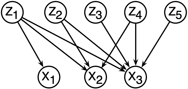
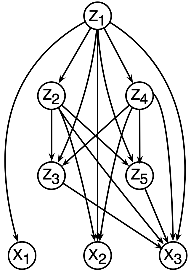
For example, consider a prominent example of a BN in Figure 1 (1i), commonly known as a hidden Markov model (HMM). In Figure 1 (1ii), we see the result of VErto, followed by marginalization of , , and deeming these three variables latent. This SPN shall be converted back into a BN. In Figure 2 (2i, 2ii) we see the BNs produced by Zhao et al. (2015) and Peharz et al. (2017), respectively. Both BNs introduce more variables than were present originally, and the introduced edges hardly reflect the succinct independence assumptions of the HMM. In Figure 2 (2iii), the decompilation result by our SPN2BN algorithm is depicted. It can be seen that SPN2BN recovers the original HMM structure, where latent variables , , and exactly correspond to the original latent variables , and , respectively. Evidently, no decompilation is able to recover the original labels for these variables, since reference to these has been explicitly removed by the previous (optional) marginalization operation. However, we see that SPN2BN successfully detects their signature in the compiled SPN, enabling it to recover an equivalent set of latent variables.


2 Sum-Product Networks
Here, we review BNs, ACs, and SPNs, as well as the compilation of BNs into SPNs.
We denote random variables (RVs) by uppercase letters, such as and , possibly with subscripts, and their values by corresponding lowercase letters and . Sets of RVs are denoted by boldfaced uppercase letters and their combined values by corresponding boldfaced lowercase letters. The children of a variable in a directed acyclic graph (DAG) , denoted , are the immediate descendants of in . Similarly, the parents of a variable are immediate ancestors of in . The descendants are the variables with a directed path from to in . The ancestors of are similarly defined. A variable is called a v-structure in a DAG , if directed edges and appear in , where and are non-adjacent variables in .
The independency information encoded in a DAG can be read graphically by the d-separation algorithm in linear time Geiger et al. (1989).
Definition 1
Pearl (1988) If , , and are three disjoint subsets of nodes in a DAG , then is said to d-separate from , denoted , if along every path between a node in and a node in there is a node satisfying one of the following two conditions: (i) is a v-structure and neither nor any of its descendants are in , or (ii) is not a v-structure and is in .
The next definition formalizes when a DAG is an I-map of a joint probability distribution (JPD).
Definition 2
Darwiche (2009) Let be a DAG and be a JPD over the same set of variables. is an I-map of if and only if every conditional independence read by d-separation on holds in the distribution . An I-map is minimal, if ceases to be an I-map when we delete any edge from .
BNs are DAGs with nodes representing variables and edges representing variable dependencies, in which the strength of these relationships are quantified by conditional probability tables (CPTs). More formally, a BN over variables has its CPTs defined over each variable given its parents, that is, , for every . One salient feature is that the product of the BN CPTs yields a JPD over .
Definition 3
Pearl (1988) Given a JPD on a set of variables , a DAG is called a Bayesian network (BN) of if is a minimal I-map of .
In a BN, the independencies read by d-separation in the DAG are guaranteed to hold in the JPD . Unfortunately, while BNs have clear interpretability, exact inference in BNs is NP-hard Cooper (1990).
BNs can be compiled into Arithmetic Circuits (ACs) Darwiche (2003) by graphically mapping the operations performed when marginalizing all variables from the BN.
Definition 4
Darwiche (2003) An arithmetic circuit (AC) over variables is a rooted DAG whose leaf nodes are labeled with numeric constants, called parameters, or variables, called indicators, and whose other nodes are labeled with multiplication and addition operations.
Notice that parameter variables are set according to the BN CPTs, while indicator variables are set according to any observed evidence.
SPNs are a probabilistic graphical model that can be learned from data using, for instance, the LearnSPN algorithm Gens and Domingos (2013).
Definition 5
Poon and Domingos (2011) A sum-product network (SPN) is a DAG containing three types of nodes: leaf distributions, sums, and products. Leaves are tractable distribution functions over . Sum nodes compute weighted sums , where are the children of and are weights that are assumed to be non-negative and normalized Peharz et al. (2015). Product nodes compute . The value of an SPN, denoted , is the value of its root.
The scope of a sum or product node is recursively defined as , while the scope of a leaf distribution is the set of variables over which the distribution is defined. A valid SPN defines a JPD and allows for efficient inference Poon and Domingos (2011). The following two structural constraints on the DAG guarantee validity. An SPN is complete if, for every sum node, its children have the same scope. An SPN is decomposable if, for every product node, the scopes of its children are pairwise disjoint. Valid SPNs are of particular interest because they represent a JPD over the variables in the problem domain. In addition, like ACs, exact inference is linear in the size of the DAG. Unlike ACs, however, SPNs allow for a latent variable (LV) interpretation Peharz et al. (2017).
In Poon and Domingos (2011), it was suggested that SPNs can be interpreted as hierarchical latent variable model, where each sum node corresponds to a latent, marginalized random variable. This interpretation can be made explicit, by incorporating the latent variables explicitly in the SPN, yielding the so-called augmented SPN Peharz et al. (2017). We briefly review the construction of the augmented SPN here: first, for each sum node we postulate a random variable with states, i.e. each state of corresponds to one of ’s children. The states of are represented via indicators , which are explicitly introduced in the SPN. Furthermore, the sum node is replaced with . This construction, originally proposed by Poon and Domingos (2011), allows us to switch ’s children “off and on” by setting the indicators of , and therefore interpret the children as distributions, conditioned on .
However, as observed in Peharz et al. (2017), this construction is in conflict with the completeness requirement of SPNs. Consider a sum node with the property that it has a child which does not reach , i.e., . Peharz et al. (2017) call such a contitioning sum of . Including the indicators as above renders incomplete, since some but not all children of reach . This has the severe consequence that the tractable inference mechanism for SPNs is now invalid. Peharz et al. (2017) propose to fix this problem by introducing a new (dummy) sum node , which has only the indicators , as children, the so-called twin sum of . Each child which does not reach is now replaced with . As shown in Peharz et al. (2017), this process leads to a consistent augmentation of the SPN in that sense that it explicitly manifests a random variable for , while i) maintaining completeness and decomposability, and ii) leaving the marginal distribution over observed variables unchanged. For further details, see Peharz et al. (2017), in particular Algorithm AugmentSPN.
3 SPN Decompilation
In this section, we formalize SPN decompilation into a BN.
The interpretation of SPNs as latent variable models is not unique. For instance, every SPN sum node can be viewed itself as a LV, as done in Zhao et al. (2015); Peharz et al. (2015). In stark contrast, all SPN sum nodes can be interpreted as one single LV Peharz (2015). This provides a wide spectrum of interpretations based only on those sum nodes appearing in an SPN. In addition, external LVs can be introduced to an SPN, such as the switching parents in Peharz et al. (2015). Thus, for a given SPN learned from data, there are seemingly countless possible interpretations of its latent space.
The approach taken in this paper is to make a compilation assumption, i.e., to assume that there exist some underlying BN which was compiled into the SPN at hand. While there are many possible ways to compile a BN into an SPN, we use arguably the most prominent compilation method, Variable Elimination (VE) Zhang and Poole (1994) following any reverse topological order (VErto). In particular, the recursive marginalization of variables during VE generate hierarchical layers of sum nodes, which typically appear in SPNs. Besides assuming that the underlying SPN was generated from a BN, we further assume that some of the BN’s variables have been removed, that is, marginalized from the model. The task of decompilation can than be formulated to recover the original BN structure as far as possible. The main contributions in this paper are to i) provide such an algorithm SPN2BN, and ii) show that it indeed recovers the morally closed version of the original BN (see Definition 11 for moral closure).
Algorithm 1 describes our compilation assumption, VErto followed by optionally marginalizing some variables. In line 4, a given BN B is converted into an A using VErto Darwiche (2003). In line 6, the leaf parameters are redistributed as sum-weights Rooshenas and Lowd (2014), yielding an SPN . In line 7, we assume that all internal latent variables in are marginalized and, thus, all of their indicator variables are set to 1. Here, any arbitrary subset of the internal latent variables can be considered. Next, we recursively simplify by applying three operations until no further change can be made. In line 11, a sum node with only indicator nodes as children is converted into a terminal node Zhao et al. (2015), which is a univariate distribution over the indicator variable. Product nodes whose children are exclusively products, i.e., chains of products are simplified into a single product node in line 12. Finally, in line 14, if two or more product nodes have the same set of children, then they are lumped into a single product node.
On the other hand, by decompilation, we mean the procedure of converting an SPN into a BN. This process involves determining the RVs and DAG for the BN. We can suggest RVs for the BN by analyzing the compilation assumption. Similarly, an I-map can be obtained as a DAG using the SPN DAG. We now formalize these ideas.
Definition 6
Given an SPN over RVs and a compilation assumption, SPN decompilation is an algorithm that both: (i) suggests a set of LVs , and; (ii) produces an I-map over and .
Task (i) of SPN decompilation is more involved than expected. A naive approach is to disregard the compilation assumption and treat each sum node as one LV. Negative consequences of this approach will be discussed in the next section. We suggest a more elegant approach by interpreting the effect of the compilation assumption on the graphical characteristics of the SPN.
Recall that we assume the SPN was compiled using VErto. During compilation, marginalizing variables creates groups of sum nodes in the same layer (the distance of the longest path from the root). Hence, identifying these groups is a way of suggesting RVs for the decompiled BN.
More formally, given a sum node , the sum-depth of is the number of sum nodes in the longest directed path from the root to .
Example 1
A sum-layer is the set of all sum nodes having the same sum-depth.
Example 2
A sum-region is the set of all sum-nodes within the same sum-layer and having the same scope.
Example 3
A sum-region is created by marginalizing variables during our compilation assumption. Thus, to answer task (i) of SPN decompilation, we suggest that consists of one LV per sum-region.
We now turn our attention to task (ii) of SPN decompilation, that is, constructing an I-map over and . Augment the SPN as done in Peharz et al. (2017). However, before continuing, we need to correct the notion of a conditioning sum node for the following reason. Consider sum node in the SPN of Figure 1 (1ii). Peharz et al. (2017) would not define sum node as a conditioning sum node for , even though would appear as a conditioning variable for in the CPT , as depicted in the constructed I-map in Figure 2 (2ii).
Definition 7
An ancestor sum node of a node in an augmented SPN is called conditioning, if it is not true that all children of reach exactly the same subset of and .
Example 5
In Example 5, observe that is not a conditioning sum node for and hence does not appear as parent of in our constructed I-map in Figure 2 (2iii).
The SPN decompilation techniques described thus far are formalized as Algorithm 2.
4 Theoretical Foundation
In this section, we first establish important properties of SPN decompilation. Later, we show a favorable characteristic of our compilation assumption and Algorithm 2.
4.1 On SPN Decompilation
Our decompilation algorithm is parsimonious with the introduction of LVs. One LV is assigned per sum-region rather than one per sum node.
Regarding I-map construction, we first show the correctness of the I-map, and then establish that the constructed I-map is minimal.
The I-map correctness follows from the CPT construction suggested in Peharz et al. (2017). Theorem 1 in Peharz et al. (2017) shows that certain independencies necessarily hold in an SPN, namely, each LV for a sum node is conditionally independent of all non-descendant sum nodes given all ancestor sum nodes of , denoted . A CPT is constructed for their I-map. The I-map built in Algorithm 2 uses the same CPT probability values, except building the CPT , where are those conditioning nodes defined in Definition 7. Since , the independencies encoded in the I-map of Peharz et al. (2017) are a subset of those encoded by the I-map built by Algorithm 2. Thus, the I-maps proposed in Peharz et al. (2017) are, in general, not minimal.
Example 7
The proof for these new conditional independencies and the correctness of our I-map is formalized in Lemma 8.
Lemma 8
Consider an augmented SPN with a sum node . Let be all of ’s ancestors and all of ’s conditioning sum nodes. Then, .
Proof
Let be the non-conditioning ancestor sum nodes of .
While conditioning on selects a single path in the augmented SPN from the root to , multiple paths may exist from the root to when conditioning only on .
By Definition 7, however, all children of a non-conditioning node reach the same subset of and .
Therefore, the weight corresponding to the instantiation of necessarily appears in every term of products in the summation.
By the distributive law, can be pulled out of this summation of products.
The resulting summation of products is precisely the SPN computation for the probability of the conditioning event.
Hence, these two summation of products cancel each other out leaving the conditional probability of to be .
Thus, .
We next show that our constructed I-maps are minimal.
Theorem 9
Let be an augmented SPN over RVs and LVs . Given as input, the algorithm SPN2BN builds a minimal I-map.
Proof By contradiction, suppose that the constructed I-map is not minimal. Then there exists a directed edge from a conditioning node for a sum node that can be deleted without destroying I-mapness. In particular, this means that
| (1) |
By Definition 7, as is a conditioning sum for , there exist at least two children and of that select different paths to and its twin .
Since the respective weights and of and can be different, it immediately follows that Equation (1) is not satisfied by the joint probability distribution defined by .
Thus, the I-mapness is violated, if is removed from .
Therefore, by contradiction, is a minimal I-map.
4.2 Compilation and Decompilation
In this section, we first show that BN2SPN2BN, our compilation-decompilation algorithm, constructs a unique BN for a given set of original BNs. A consequence of this is that BN2SPN2BN is idempotent.
We next show that the BN output by BN2SPN2BN can be different than the original BN. In the reminder of this section, we assume is a fixed topological ordering of a given BN .
Example 8
Consider the call BN2SPN2BN(), where BN has directed edges , . Then, the output BN has directed edges , .
Notice that the directed edges of the original BN are a subset of those in the output BN.
Definition 10
A directed moralization edge is a directed edge added between two non-adjacent vertices and in a given BN whenever there exists a variable such that and , where .
We now introduce the key notion of moral closure.
Definition 11
Given a BN and a fixed topological order of , the moral closure of , denoted , is the unique BN formed by iteratively augmenting with all directed moralization edges.
We are now ready to present the first main result of our compilation-decompilation process.
Theorem 12
Given a BN and a fixed topological order of , the output of the compilation-decompilation algorithm BN2SPN2BN is the moral closure of .
Proof Applying BN2SPN2BN on involves running BN2SPN followed by SPN2BN. Consider running BN2SPN on . This involves eliminating all variables from following an elimination ordering . It is well-known that this process builds a triangulated, undirected graph Pearl (1988). Triangulated, undirected graphs admit a perfect numbering. This means that no fill-in edges need to be added to the triangulated, undirected graph when eliminating variables following the perfect numbering.
Now itself is a perfect numbering for the triangulated graph built by eliminating variable following . Let us focus on the undirected edges that were added to . There are two cases to consider, i.e., moralization edges and triangulation edges. A moralization edge corresponds to a directed moralization edge in our case.
A triangulation edge is added if and only if and are non-adjacent parents of a common child in the directed case.
However, these edges are precisely the directed moralization edges that are recursively added.
Therefore, BN2SPN builds an SPN following the hierarchy in the moral closure of and subsequently SPN2BN unwinds the SPN following this same hierarchy.
Thus, given , BN2SPN2BN yields the moral closure of .
Theorem 12 has a couple of important consequences. As Theorem 12 establishes that the output of BN2SPN2BN is the moral closure of the input BN , it immediately follows that the output BN is exactly the input BN whenever no directed moralization edges are added to . One situation where this occurs is when does not have any v-structures, such as in the case of HMMs. Here, , so the output BN of BN2SPN2BN is the same as the input (up to a relabelling of variables). For example, recall the HMM in Figure 1 (1i). BN2SPN2BN yielded back the same BN as illustrated in Figure 2 (2iii). A second important case is when the input is itself. This leads to out next result showing that our compilation-decompilation process is idempotent.
Theorem 13
BN2SPN2BN is idempotent.
Proof
Let be a BN and a fixed topological ordering of .
Then , by Theorem 12.
By definition, the moral closure of is itself.
Thus, .
Therefore, BN2SPN2BN is idempotent.
Theorem 13 has practical significance because it limits the maximum size of the decompiled BN to be the size of the moral closure of the input BN. In contrast, if we change the decompilation method to Zhao et al. (2015) or Peharz et al. (2017), then applying BN2SPN2BN repeatedly will continually yield a larger BN.
5 Conclusion
In this paper, we formalize SPN decompilation by suggesting SPN2BN, an algorithm that converts an SPN into a BN. SPN2BN is an improvement over Zhao et al. (2015) and Peharz et al. (2017), which are excessive with the number of introduced latent variables. One key result of our SPN decompilation is that it constructs the moral closure of the original BN . This means that in certain cases like for HMMs, where the moral closure of a BN is itself, our SPN decompilation will return the original BN. Moreover, our compilation-decompilation process is idempotent. This has practical significance as it limits the maximum size of the decompiled BN to be the size of .
References
- Boutilier et al. (1996) C. Boutilier, N. Friedman, M. Goldszmidt, and D. Koller. Context-specific independence in Bayesian networks. In Proceedings of the Twelfth Conference on Uncertainty in Artificial Intelligence, pages 115–123, 1996.
- Choi and Darwiche (2017) A. Choi and A. Darwiche. On relaxing determinism in arithmetic circuits. In Proceedings of the 34th International Conference on Machine Learning-Volume 70, pages 825–833, 2017.
- Cooper (1990) G. Cooper. The computational complexity of probabilistic inference using Bayesian belief networks. Artificial Intelligence, 42(2-3):393–405, 1990.
- Darwiche (2003) A. Darwiche. A differential approach to inference in Bayesian networks. Journal of the ACM, 50(3):280–305, 2003.
- Darwiche (2009) A. Darwiche. Modeling and Reasoning with Bayesian Networks. Cambridge University Press, Los Angeles, CA, 2009.
- Geiger et al. (1989) D. Geiger, T. S. Verma, and J. Pearl. d-separation: From theorems to algorithms. In Proceedings of the Fifth Conference on Uncertainty in Artificial Intelligence, pages 139–148, 1989.
- Gens and Domingos (2013) R. Gens and P. Domingos. Learning the structure of sum-product networks. In Proceedings of the Thirtieth International Conference on Machine Learning, pages 873–880, 2013.
- Koller and Friedman (2009) D. Koller and N. Friedman. Probabilistic Graphical Models: Principles and Techniques. MIT Press, Cambridge, MA, 2009.
- Pearl (1988) J. Pearl. Probabilistic Reasoning in Intelligent Systems: Networks of Plausible Inference. Morgan Kaufmann, San Francisco, CA, 1988.
- Peharz (2015) R. Peharz. Foundations of sum-product networks for probabilistic modeling. PhD thesis, 2015.
- Peharz et al. (2015) R. Peharz, S. Tschiatschek, F. Pernkopf, and P. Domingos. On theoretical properties of sum-product networks. In Proceedings of the Eighteenth International Conference on Artificial Intelligence and Statistics, pages 744–752, 2015.
- Peharz et al. (2017) R. Peharz, R. Gens, F. Pernkopf, and P. Domingos. On the latent variable interpretation in sum-product networks. IEEE Transactions on Pattern Analysis and Machine Intelligence, 39(10):2030–2044, 2017.
- Poon and Domingos (2011) H. Poon and P. Domingos. Sum-product networks: A new deep architecture. In Proceedings of the Twenty-Seventh Conference on Uncertainty in Artificial Intelligence, pages 337–346, 2011.
- Rooshenas and Lowd (2014) A. Rooshenas and D. Lowd. Learning sum-product networks with direct and indirect variable interactions. In Proceedings of the Thirty-First International Conference on Machine Learning, pages 710–718, 2014.
- Zhang and Poole (1994) N. L. Zhang and D. Poole. A simple approach to Bayesian network computations. In Proceedings of the Tenth Canadian Artificial Intelligence Conference, pages 171–178, 1994.
- Zhao et al. (2015) H. Zhao, M. Melibari, and P. Poupart. On the relationship between sum-product networks and Bayesian networks. In Proceedings of Thirty-Second International Conference on Machine Learning, pages 116–124, 2015.