Improving ADMMs for Solving Doubly Nonnegative Programs through Dual Factorization

Abstract

Alternating direction methods of multipliers (ADMMs) are popular approaches to handle large scale semidefinite programs that gained attention during the past decade. In this paper, we focus on solving doubly nonnegative programs (DNN), which are semidefinite programs where the elements of the matrix variable are constrained to be nonnegative. Starting from two algorithms already proposed in the literature on conic programming, we introduce two new ADMMs by employing a factorization of the dual variable.

It is well known that first order methods are not suitable to compute high precision optimal solutions, however an optimal solution of moderate precision often suffices to get high quality lower bounds on the primal optimal objective function value. We present methods to obtain such bounds by either perturbing the dual objective function value or by constructing a dual feasible solution from a dual approximate optimal solution. Both procedures can be used as a post-processing phase in our ADMMs.

Numerical results for DNNs that are relaxations of the stable set problem are presented. They show the impact of using the factorization of the dual variable in order to improve the progress towards the optimal solution within an iteration of the ADMM. This decreases the number of iterations as well as the CPU time to solve the DNN to a given precision. The experiments also demonstrate that within a computationally cheap post-processing, we can compute bounds that are close to the optimal value even if the DNN was solved to moderate precision only. This makes ADMMs applicable also within a branch-and-bound algorithm.

1 Introduction

In a semidefinite program (SDP) one wants to find a positive semidefinite (and hence symmetric) matrix such that linear – in the entries of the matrix – constraints are fulfilled and a linear objective function is minimized. If the matrix is also required to be entrywise nonnegative, the problem is called doubly nonnegative program (DNN). Since interior point methods fail (in terms of time and memory required) when the scale of the SDP is big, augmented Lagrangian approaches became more and more popular to solve this class of programs. Wen, Goldfarb and Yin [15] as well as Malick, Povh, Rendl and Wiegele [11] and De Santis, Rendl and Wiegele [3] considered alternating direction methods of multipliers (ADMMs) to solve SDPs. One can directly apply these ADMMs to solve DNNs, too, by introducing nonnegative slack variables for the nonnegativity constraints in order to obtain equality constraints only. However, this increases the size of the problem significantly.

In this paper, we first present two ADMMs already proposed in the literature (namely ConicADMM3c by Sun, Toh and Yang [14] and ADAL+ [15]) to specifically solve DNNs. Then we introduce two new methods: DADMM3c, which employs a factorization of the dual matrix to avoid spectral decompositions, and DADAL+ taking advantage of the practical benefits of DADAL [3]. Note that there are examples for which a 3-block ADMM (like DADAL+) diverges. However, the question of convergence of 3-block ADMMs for SDP relaxations arising from combinatorial optimization problems is still open.

In case the DNN is used as relaxation of some combinatorial optimization problem, one is interested in dual bounds, i.e. bounds that are the dual objective function value of a dual feasible solution. In case of a minimization problem this is a lower bound, in case of a maximization problem an upper bound. Having bounds is in particular important if one intends to use the relaxation within a branch-and-bound algorithm. This, however, means that one needs to solve the DNN to high precision such that the dual solution is feasible and hence the dual objective function value is a reliable bound. Typically, first order methods can compute solutions of moderate precision in reasonable time, whereas progressing to higher precision can become expensive. To overcome this drawback, we present two methods to compute a dual bound from a solution obtained by the ADMMs within a post-processing phase.

In the following section we state our notations and introduce the formulation of standard primal-dual SDPs and DNNs. In Section 2 we go through the two existing ADMMs for DNNs we mentioned before, and in Section 3 we introduce the tool of dual matrix factorization used in the new ADMMs DADAL+ and DADMM3c presented later in the same section. In Section 4 we present two methods for obtaining dual bounds from a solution of a DNN that satisfies the optimality criteria to moderate precision only. Section 5 shows numerical results for instances of DNN relaxations of the stable set problem. We evaluate the impact of the dual factorization within the methods as well as the two post-processing schemes for obtaining dual bounds. Section 6 concludes the paper.

1.1 Problem Formulation and Notations

Let ${\mathscr{S}}_{n}$ be the set of $n$-by-$n$ symmetric matrices, ${\mathscr{S}}_{n}^{+}~{}\subset~{}{\mathscr{S}}_{n}$ be the set of positive semidefinite matrices and ${\mathscr{S}}_{n}^{-}~{}\subset~{}{\mathscr{S}}_{n}$ be the set of negative semidefinite matrices. Denoting by $\left\langle X,Y\right\rangle={\rm trace}(XY)$ the standard inner product in ${\mathscr{S}}_{n}$, we write the standard primal-dual pair of SDPs as

$$\min\, \left\langle C,X\right\rangle$$ (1)

s.t. $${\mathscr{A}}X=b$$

$$X\in{\mathscr{S}}_{n}^{+}$$

and

$$\max\, b^{T}y$$ (2)

s.t. $${\mathscr{A}}^{\top}y+Z=C$$

$$Z\in{\mathscr{S}}_{n}^{+},$$

where $C\in{\mathscr{S}}_{n}$, $b\in\mathbb{R}^{m}$, ${\mathscr{A}}:{\mathscr{S}}_{n}\rightarrow\mathbb{R}^{m}$ is the linear operator $({\mathscr{A}}X)_{i}=\left\langle A_{i},X\right\rangle$ with $A_{i}\in{\mathscr{S}}_{n}$, $i=1,\ldots,m$ and ${\mathscr{A}}^{\top}:\mathbb{R}^{m}\rightarrow{\mathscr{S}}_{n}$ is its adjoint operator, so ${\mathscr{A}}^{\top}y=\sum_{i}y_{i}A_{i}$ for $y\in\mathbb{R}^{m}$.

When in the primal SDP (1) the elements of $X$ are constrained to be nonnegative, then the SDP is called a doubly nonnegative program (DNN). To be more precise the primal DNN is given as

$$\min\, \left\langle C,X\right\rangle$$ (3)

s.t. $${\mathscr{A}}X=b$$

$$X\in{\mathscr{S}}_{n}^{+},\quad X\geq 0.$$

Introducing $S$ as the dual variable related to the nonnegativity constraint $X\geq 0$, we write the dual of the DNN (3) as

$$\max\, b^{T}y$$ (4)

s.t. $${\mathscr{A}}^{\top}y+Z+S=C$$

$$Z\in{\mathscr{S}}_{n}^{+},\quad S\in{\mathscr{S}}_{n},\quad S\geq 0.$$

We assume that both the primal DNN (3) and the dual DNN (4) have strictly feasible points (i.e. Slater’s condition is satisfied), so strong duality holds. Under this assumption, $(y,S,Z,X)$ is optimal for (3) and (4) if and only if

$${\mathscr{A}}X =b,\quad {\mathscr{A}}^{\top}y+Z+S =C,\quad ZX =0,$$ (5)

$$X \in{\mathscr{S}}_{n}^{+},\quad Z \in{\mathscr{S}}_{n}^{+},\quad \left\langle S,X\right\rangle =0,$$

$$X \geq 0,\quad S\in{\mathscr{S}}_{n},\quad S \geq 0,$$

hold. We further assume that the constraints formed through the operator ${\mathscr{A}}$ are linearly independent.

Let $v\in\mathbb{R}^{n}$ and $M\in\mathbb{R}^{m\times n}$. In the following, $M(i,:)$ is defined as the i-th row of $M$ and $M(:,j)$ as the j-th column of $M$. Further we denote by ${\rm Diag}{(v)}$ the diagonal matrix having $v$ on the main diagonal. The vector $e_{i}$ is defined as the $i$-th vector of the standard basis in $\mathbb{R}^{n}$. Whenever a norm is used, we consider the Frobenius norm in case of matrices and the Euclidean norm in case of vectors. Let $S\in{\mathscr{S}}_{n}$. We denote the projection of $S$ onto the positive semidefinite and negative semidefinite cone by $(S)_{+}$ and $(S)_{-}$, respectively. The projection of $S$ onto the nonnegative orthant is denoted by $(S)_{\geq 0}$. Moreover we denote by $\lambda(S)$ the vector of the eigenvalues of $S$ and by $\lambda_{\min}(S)$ and $\lambda_{\max}(S)$ the smallest and largest eigenvalue of $S$, respectively.

2 ADMMs for Doubly Nonnegative Programs

In this section, we present two different ADMMs for solving DNNs. Let $X\in{\mathscr{S}}_{n}$ be the Lagrange multiplier for the dual equation ${\mathscr{A}}^{\top}y+Z+S-C=0$ and $\sigma>0$ be fixed. Then the augmented Lagrangian of the dual DNN (4) is defined as

$$L_{\sigma}(y,S,Z;X)=b^{T}y-\langle{\mathscr{A}}^{\top}y+Z+S-C,X\rangle-\frac{\sigma}{2}\|{\mathscr{A}}^{\top}y+Z+S-C\|^{2}.$$

In the classical augmented Lagrangian method applied to the dual DNN (4) the problem

$$\max\, L_{\sigma}(y,S,Z;X)$$ (6)

s.t. $$y\in\mathbb{R}^{m},\quad S\in{\mathscr{S}}_{n},\quad S\geq 0,\quad Z\in{\mathscr{S}}_{n}^{+},$$

where $X$ is fixed and $\sigma>0$ is a penalty parameter is addressed at every iteration.

Once Problem (6) is (approximately) solved, the multiplier $X$ is updated by the first order rule

$$X=X+\sigma({\mathscr{A}}^{\top}y+Z+S-C)$$ (7)

and the process is iterated until convergence, i.e., until the optimality conditions (5) are satisfied within a certain tolerance (see [1, Chapter 2] for further details).

If the augmented Lagrangian $L_{\sigma}(y,S,Z;X)$ is maximized with respect to $y$, $S$ and $Z$ not simultaneously but one after the other, this yields the well known alternating direction method of multipliers (ADMM). The number of blocks of an ADMM is the number of blocks of variables for which Problem (6) is maximized separately, so we consider a 3-block ADMM. Such an ADMM has been specialized and used by Wen, Goldfarb and Yin [15] to address DNNs and in the following we refer to this method as ADAL+. Details will be given in Section 2.1. Even though in all our numerical tests this algorithm reaches the desired precision of our stopping criteria, it has been recently shown in [2] that an ADMM with more than two blocks may diverge.

In order to overcome this theoretical issue, Sun, Toh and Yang [14] proposed to update the third block twice per iteration, or, in other words, to maximize $L_{\sigma}(y,S,Z;X)$ with respect to the variable $y$ two times in one iteration. Their algorithm, named ConicADMM3c and detailed in Section 2.2, is the first theoretically convergent 3-block ADMM proposed in the context of conic programming.

2.1 ADAL+

In the following, we refer to the ADMM presented by Wen, Goldfarb and Yin in [15] and applied to the dual DNN (4) as ADAL+. As already mentioned, ADAL+ iterates the maximization of the augmented Lagrangian with respect to each block of dual variables. To be more precise the new point $(y^{k+1},S^{k+1},Z^{k+1},X^{k+1})$ is computed by the following steps:

$$y^{k+1} =\operatorname*{arg\,max}_{y\in\mathbb{R}^{m}}L_{\sigma^{k}}(y,S^{k},Z^{k};X^{k}),$$ (8)

$$S^{k+1} =\operatorname*{arg\,max}_{S\in{\mathscr{S}}_{n},S\geq 0}L_{\sigma^{k}}(y^{k+1},S,Z^{k};X^{k}),$$ (9)

$$Z^{k+1} =\operatorname*{arg\,max}_{Z\in{\mathscr{S}}_{n}^{+}}L_{\sigma^{k}}(y^{k+1},S^{k+1},Z;X^{k}),$$ (10)

$$X^{k+1} =X^{k}+\sigma^{k}({\mathscr{A}}^{\top}y^{k+1}+Z^{k+1}+S^{k+1}-C).$$ (11)

The update of $y$ in (8) is derived from the first-order optimality condition of the problem on the right-hand side of (8), so $y^{k+1}$ is the unique solution of

$$\nabla_{y}L_{\sigma^{k}}(y,S^{k},Z^{k};X^{k})=b-{\mathscr{A}}(X^{k}+\sigma^{k}({\mathscr{A}}^{\top}y+Z^{k}+S^{k}-C))=0,$$

that is

$$y^{k+1}=({\mathscr{A}}{\mathscr{A}}^{\top})^{-1}\Big{(}\frac{1}{\sigma^{k}}b-{\mathscr{A}}(\frac{1}{\sigma^{k}}X^{k}+Z^{k}+S^{k}-C)\Big{)}.$$

As shown in [15], the update of $S$ according to (9) is equivalent to

$$\min_{S\in{\mathscr{S}}_{n},S\geq 0}\|S-U^{k+1}\|^{2},$$

where $U^{k+1}=C-{\mathscr{A}}^{\top}y^{k+1}-Z^{k}-\frac{1}{\sigma^{k}}X^{k}$. Hence, $S^{k+1}$ is obtained as the projection of $U^{k+1}$ onto the nonnegative orthant, namely

$$S^{k+1}=\big{(}U^{k+1}\big{)}_{\geq 0}=\big{(}C-{\mathscr{A}}^{\top}y^{k+1}-Z^{k}-\frac{1}{\sigma^{k}}X^{k}\big{)}_{\geq 0}.$$

Then, the update of $Z$ in (10) is conducted by considering the equivalent problem

$$\min_{Z\in{\mathscr{S}}_{n}^{+}}\|Z+W^{k+1}\|^{2},$$ (12)

with $W^{k+1}=(\frac{1}{\sigma^{k}}X^{k}-C+{\mathscr{A}}^{\top}y^{k+1}+S^{k+1})$, or, in other words, by projecting $W^{k+1}\in{\mathscr{S}}_{n}$ onto the (closed convex) cone ${\mathscr{S}}_{n}^{-}$ and taking its additive inverse (see Algorithm 1). Such a projection is computed via the spectral decomposition of the matrix $W^{k+1}$.

Finally, it is easy to see that the update of $X$ in (11) can be performed considering the projection of $W^{k+1}\in{\mathscr{S}}_{n}$ onto ${\mathscr{S}}_{n}^{+}$ multiplied by $\sigma^{k}$, namely

$$X^{k+1} =X^{k}+\sigma^{k}({\mathscr{A}}^{\top}y^{k+1}+Z^{k+1}+S^{k+1}-C)=$$

$$=\sigma^{k}(X^{k}/\sigma^{k}-C+{\mathscr{A}}^{\top}y^{k+1}+S^{k+1}-(X^{k}/\sigma^{k}-C+{\mathscr{A}}^{\top}y^{k+1}+S^{k+1})_{-})=$$

$$=\sigma^{k}(X^{k}/\sigma^{k}-C+{\mathscr{A}}^{\top}y^{k+1}+S^{k+1})_{+}.$$

We report in Algorithm 1 the scheme of ADAL+.

Algorithm 1 Scheme of ADAL+ from [15]

1:Choose $\sigma>0$, $\varepsilon>0$, $X\in{\mathscr{S}}_{n}^{+}$, $Z\in{\mathscr{S}}_{n}^{+}$, $S\in{\mathscr{S}}_{n}$ with $S\geq 0$

2:$\delta=\max\{r_{P},r_{D},r_{PP},r_{CS}\}$

3:while $\delta>\varepsilon$ do

4:     $y=({\mathscr{A}}{\mathscr{A}}^{\top})^{-1}\Big{(}\frac{1}{\sigma}b-{\mathscr{A}}(\frac{1}{\sigma}X-C+Z+S)\Big{)}$

5:     $S=(C-{\mathscr{A}}^{\top}y-Z-\frac{1}{\sigma}X)_{\geq 0}$

6:     $Z=-(X/\sigma-C+{\mathscr{A}}^{\top}y+S)_{-}$ and $X=\sigma(X/\sigma-C+{\mathscr{A}}^{\top}y+S)_{+}$

7:     $\delta=\max\{r_{P},r_{D},r_{PP},r_{CS}\}$

8:     Update $\sigma$

9:end while

The stopping criterion of ADAL+ considers the following errors

$$r_{P} =\frac{\|{\mathscr{A}}X-b\|}{1+\|b\|},\quad\quad r_{D} =\frac{\|{\mathscr{A}}^{\top}y+Z+S-C\|}{1+\|C\|},$$

$$r_{PP} =\frac{\|X-(X)_{\geq 0}\|}{1+\|X\|},\quad\quad r_{CS} =\frac{|\left\langle S,X\right\rangle|}{1+\|X\|+\|S\|},$$

related to primal feasibility (${\mathscr{A}}X=b$, $X\geq 0$), dual feasibility (${\mathscr{A}}^{\top}y+Z+S=C$) and complementarity condition ($\left\langle S,X\right\rangle=0$). More precisely, the algorithm stops as soon as the quantity

$$\delta=\max\{r_{P},r_{D},r_{PP},r_{CS}\}$$

is less than a fixed precision $\varepsilon>0$.

The other optimality conditions (namely $X\in{\mathscr{S}}_{n}^{+}$, $Z\in{\mathscr{S}}_{n}^{+}$, $S\in{\mathscr{S}}_{n}$, $S\geq 0$, $ZX=0$) are satisfied up to machine accuracy throughout the algorithm thanks to the projections employed in ADAL+.

2.2 ConicADMM3c

A major drawback of ADAL+ is that it is not necessarily convergent. By considering two updates of the variable $y$ within one iteration, Sun, Toh and Yang are able to prove that the algorithm ConicADMM3c proposed in [14] and detailed in Algorithm 2 is a 3-block convergent ADMM: Under certain assumptions, they show that the sequence $\{(y^{k},S^{k},Z^{k};X^{k})\}$ produced by ConicADMM3c converges to a KKT point of the primal DNN (3) and the dual DNN (4). Note that also the order of the updates on the blocks of variables is different with respect to ADAL+. The convergence analysis is based on the fact that ConicADMM3c is equivalent to a semi-proximal ADMM.

With respect to ADAL+, ConicADMM3c has the drawback that fewer optimality conditions are satisfied up to machine accuracy throughout the algorithm. Additionally to $r_{P},r_{D},r_{PP}$ and $r_{CS}$, the stopping criterion of ConicADMM3c has to take into account the errors

$$r_{PD}=\frac{\|(-X)_{+}\|}{1+\|X\|}\quad\text{ and }\quad r_{CZ}=\frac{\|\left\langle Z,X\right\rangle\|}{1+\|X\|+\|Z\|},$$

related to the primal feasibility $X\in{\mathscr{S}}_{n}^{+}$ and the complementarity condition $ZX=0$. In fact, as the second update of $y$ is performed after the update of $Z$, the spectral decomposition of $W^{k+1}$ cannot be used to update $X$ as in ADAL+ and both the complementarity condition $ZX=0$ and the positive semidefiniteness of $X$ are not satisfied by construction. (We will give a summary on the conditions satisfied throughout the algorithms in Table 1 in a subsequent section.) From a computational point of view this slows down the convergence of the scheme, which will be confirmed in our computational evaluation in Section 5.

Algorithm 2 Scheme of ConicADMM3c from [14]

1:Choose $\sigma>0$, $\varepsilon>0$, $X\in{\mathscr{S}}_{n}^{+}$, $Z\in{\mathscr{S}}_{n}^{+}$, $S\in{\mathscr{S}}_{n}$ with $S\geq 0$

2:$\delta=\max\{r_{P},r_{D},r_{PP},r_{PD},r_{CS},r_{CZ}\}$

3:while $\delta>\varepsilon$ do

4:     $Z=-(X/\sigma-C+{\mathscr{A}}^{\top}y+S)_{-}$

5:     $y=({\mathscr{A}}{\mathscr{A}}^{\top})^{-1}\Big{(}\frac{1}{\sigma}b-{\mathscr{A}}(\frac{1}{\sigma}X-C+Z+S)\Big{)}$

6:     $S=(C-{\mathscr{A}}^{\top}y-Z-\frac{1}{\sigma}X)_{\geq 0}$

7:     $y=({\mathscr{A}}{\mathscr{A}}^{\top})^{-1}\Big{(}\frac{1}{\sigma}b-{\mathscr{A}}(\frac{1}{\sigma}X-C+Z+S)\Big{)}$

8:     $X=X+\sigma({\mathscr{A}}^{\top}y+Z+S-C)$

9:     $\delta=\max\{r_{P},r_{D},r_{PP},r_{PD},r_{CS},r_{CZ}\}$

10:     Update $\sigma$

11:end while

3 Dual Matrix Factorization

In this section, we present our new variants of ADAL+ and ConicADMM3c, namely DADAL+ and DADMM3c, where a factorization of the dual variable $Z$ is employed. We adapt the method introduced by De Santis, Rendl and Wiegele in [3]. In particular, we look at the augmented Lagrangian problem where the positive semidefinite constraint on the dual matrix $Z$ is eliminated by considering the factorization $Z=VV^{\top}$. To be more precise, in each iteration of the ADMMs for fixed $X$, we focus on the problem

$$\max\, L_{\sigma}(y,S,V;X)$$ (13)

s.t. $$y\in\mathbb{R}^{m},\quad S\in{\mathscr{S}}_{n},\quad S\geq 0,\quad V\in\mathbb{R}^{n\times r},$$

where

$$L_{\sigma}(y,S,V;X)=b^{T}y-\langle{\mathscr{A}}^{\top}y+VV^{\top}+S-C,X\rangle-\frac{\sigma}{2}\|{\mathscr{A}}^{\top}y+VV^{\top}+S-C\|^{2}.$$

Compared to (6) the constraint $Z\in{\mathscr{S}}_{n}^{+}$ is replaced by $Z=VV^{\top}$ for some $V\in\mathbb{R}^{n\times r}$, so $Z\in{\mathscr{S}}_{n}^{+}$ is fulfilled automatically. Note that the number of columns $r$ of the matrix $V$ represents the rank of $Z$.

The use of the factorization of the dual variable in ADAL+ should improve the numerical performance of the algorithm when dealing with structured DNNs, as it happens in the comparison of the algorithm DADAL with ADAL when dealing with structured SDPs [3]. For what concerns ConicADMM3c, we will see in Section 3.2 that using the factorization of the dual variable allows to avoid any spectral decomposition along the iterations of the algorithm, without compromising the theoretical convergence of the method.

Note that Problem (13) is unconstrained with respect to the variables $y$ and $V$. In particular, the following holds.

Proposition 1.

Let $(y^{*},S^{*},V^{*})\in\mathbb{R}^{m}\times{\mathscr{S}}_{n}\times\mathbb{R}^{n\times r}$ be a stationary point of (13), then

$$\nabla_{y}L_{\sigma}(y^{*},S^{*},V^{*};X) =b-{\mathscr{A}}(X+\sigma({\mathscr{A}}^{\top}y^{*}+{V^{*}V^{*}}^{\top}+S-C))=0\text{ and }$$ (14)

$$\nabla_{V}L_{\sigma}(y^{*},S^{*},V^{*};X) =-2(X+\sigma({\mathscr{A}}^{\top}y^{*}+{V^{*}V^{*}}^{\top}+S-C))V^{*}=0.$$

Proposition 1 implies that fulfilling the necessary optimality conditions with respect to $y$ is equivalent to solve one system of linear equations.

As in [3], we consider Algorithm 3 in order to update $y$ and $V$ (and hence $Z$) for fixed $S$ and $X$. In particular in Algorithm 3, starting from $(y,S,V;X)$, we move $V$ along an ascent direction $D_{V}\in\mathbb{R}^{n\times r}$ with a stepsize $\alpha$. While doing this, we update $y$ in such a way that we keep its optimality conditions of (13) satisfied, so $\nabla_{y}L_{\sigma}(y,S,V+\alpha D_{V};X)=0$ holds for the updated $y$ (see [3, Proposition 2]). We stop as soon as the necessary optimality conditions with respect to $V$ (see Proposition 1) are fulfilled to a certain precision.

As in the algorithm DADAL presented in [3], in our implementation we set $D_{V}$ either to the gradient of $L_{\sigma}(y,S,V;X)$ or to the gradient scaled with the inverse of the diagonal of the Hessian of $L_{\sigma}(y,S,V;X)$. In order to determine a stepsize $\alpha$, at Step 4 in Algorithm 3 we could perform an exact linesearch to maximize $L_{\sigma}(y(V+\alpha D_{V}),S,V+\alpha D_{V};X)$ with respect to $\alpha$. This is a polynomial of degree 4 in $\alpha$, so we can interpolate it from five different points in order to get its analytical expression and by this determining the maximizer explicitly. In practice we evaluate $L_{\sigma}(y(V+\alpha D_{V}),S,V+\alpha D_{V};X)$ for 1000 different values of $\alpha\in(0,10)$ and take the $\alpha$ corresponding to the maximum value of $L_{\sigma}$.

Algorithm 3 Update of $(y,V)$ for factorization $Z=VV^{\top}$

Input: $\sigma>0$, $X\in{\mathscr{S}}_{n}^{+}$, $y\in\mathbb{R}^{m}$, $V\in\mathbb{R}^{n\times r}$, $S\in{\mathscr{S}}_{n}$ with $S\geq 0$

1:Choose $\varepsilon_{inner}>0$

2:while $\|\nabla_{V}L_{\sigma}(y,S,V;X)\|<\varepsilon_{inner}$ do

3:     Compute ascent direction $D_{V}\in\mathbb{R}^{n\times r}$

4:     Compute stepsize $\alpha$

5:     $y=y(V+\alpha D_{V})$ and $V=V+\alpha D_{V}$

6:end while

As output of Algorithm 3, we get $y$ and $V$ (and therefore also $Z=VV^{\top}$) that have been updated through the maximization of the augmented Lagrangian (13) with respect to $V$. This leads to a new point $(y,S,V;X)$.

This update can be used within ADAL+ and ConicADMM3c as detailed in the following.

3.1 DADAL+

First we consider DADAL+, our version of ADAL+ where the use of the factorization of the dual variable $Z$ leads to a double update of $Z$. As a further enhancement of the algorithm ADAL+ devised in [15], we propose to perform also a double update of the dual variable $y$.

To be more precise, we replace the first update of $y$ in ADAL+ with a update of $y$ and $V$ with Algorithm 3 in DADAL+. Furthermore in DADAL+ we update $y$ not only before, but also a second time after the computation of $S$. This second update is performed by applying the closed formula solution of the maximization problem in (8). Note that the second update of $y$ is performed before the update of $Z$ so that by computing the spectral decomposition of $W=X/\sigma-C+{\mathscr{A}}^{\top}y+S$, we can simultaneously update $Z$ and $X$ and both the complementarity condition $ZX=0$ and the positive semidefiniteness of $X$ are satisfied up to machine accuracy throughout the algorithm in the same way it is the case in ADAL+. The scheme of DADAL+ is detailed in Algorithm 4.

Algorithm 4 Scheme of DADAL+

1:Choose $\sigma>0$, $r>0$, $\varepsilon>0$, $X\in{\mathscr{S}}_{n}^{+}$, $S\in{\mathscr{S}}_{n}$ with $S\geq 0$, $V\in{\mathbb{R}}^{n\times r}$, $y\in{\mathbb{R}}^{m}$

2:$Z=VV^{\top}$

3:$\delta=\max\{r_{P},r_{D},r_{PP},r_{CS}\}$

4:while $\delta>\varepsilon$ do

5:     Update $(y,V)$ with Algorithm 3

6:     $Z=VV^{\top}$

7:     $S=(C-{\mathscr{A}}^{\top}y-Z-\frac{1}{\sigma}X)_{\geq 0}$

8:     $y=({\mathscr{A}}{\mathscr{A}}^{\top})^{-1}\Big{(}\frac{1}{\sigma}b-{\mathscr{A}}(\frac{1}{\sigma}X-C+Z+S)\Big{)}$

9:     $Z=-(X/\sigma-C+{\mathscr{A}}^{\top}y+S)_{-}$ and $X=\sigma(X/\sigma-C+{\mathscr{A}}^{\top}y+S)_{+}$

10:     $r=\mathrm{rank(Z)}$

11:     Update $V$ such that $VV^{\top}=Z$

12:     $\delta=\max\{r_{P},r_{D},r_{PP},r_{CS}\}$

13:     Update $\sigma$

14:end while

3.2 DADMM3c

We now investigate the use of the dual factorization within the algorithm ConicADMM3c and call the modified algorithm DADMM3c. In ConicADMM3c, the effort spent to compute the spectral decomposition of $W=X/\sigma-C+{\mathscr{A}}^{\top}y+S$ is not that well exploited as it is used to update only the dual matrix $Z$ but not the primal matrix $X$. Hence in DADMM3c we update $Z$ and $y$ by employing the factorization $Z=VV^{\top}$ and performing Algorithm 3 instead of updating them by a spectral decomposition and a closed formula as it is done in ConicADMM3c. Note that Algorithm 3 is able to compute stationary points of Problem (13), that are not necessarily global optima. However, assuming that the update of $y$ and $V$ at Step 5 in Algorithm 5 is done such that Problem (13) is solved to optimality, the theoretical convergence of the method is maintained. Note that the computation of any spectral decomposition is avoided. The scheme of the algorithm DADMM3c is detailed in Algorithm 5.

Algorithm 5 Scheme of DADMM3c

1:Choose $\sigma>0$, $r>0$, $\varepsilon>0$, $X\in{\mathscr{S}}_{n}^{+}$, $S\in{\mathscr{S}}_{n}$ with $S\geq 0$, $V\in{\mathbb{R}}^{n\times r}$, $y\in{\mathbb{R}}^{m}$

2:$Z=VV^{\top}$

3:$\delta=\max\{r_{P},r_{D},r_{PP},r_{PD},r_{CS},r_{CZ}\}$

4:while $\delta>\varepsilon$ do

5:     Update $(y,V)$ with Algorithm 3

6:     $Z=VV^{\top}$

7:     $S=(C-{\mathscr{A}}^{\top}y-Z-\frac{1}{\sigma}X)_{+}$

8:     $y=({\mathscr{A}}{\mathscr{A}}^{\top})^{-1}\Big{(}\frac{1}{\sigma}b-{\mathscr{A}}(\frac{1}{\sigma}X-C+Z+S)\Big{)}$

9:     $X=X+\sigma(Z+S+{\mathscr{A}}^{\top}y-C)$

10:     $\delta=\max\{r_{P},r_{D},r_{PP},r_{PD},r_{CS},r_{CZ}\}$

11:     Update $\sigma$

12:end while

A limit of DADMM3c is that the rank of $Z$ is not updated throughout the iterations. This means that the maximization of $L(y,S,V;X)$ with respect to $V$ is performed keeping $r$ fixed to the initial value that in our implementation is $n$. It is still an open question to update the rank of $Z$ in a beneficial way.

On the other hand, note that in DADAL+ the rank of $Z$ is determined at every iteration through the eigenvalue decomposition in the second update of $Z$.

As already mentioned in Section 2, some of the optimality conditions are satisfied throughout the algorithms ADAL+/DADAL+ and ConicADMM3c/DADMM3c. A summary is presented in Table 1.

	${\mathscr{A}}X=b$	$X\in{\mathscr{S}}_{n}^{+}$	$X\geq 0$	${\mathscr{A}}^{\top}y+Z+S=C$	$Z\in{\mathscr{S}}_{n}^{+}$	$S\in{\mathscr{S}}_{n}$, $S\geq 0$	$ZX=0$	$\langle S,X\rangle=0$
ADAL+ DADAL+	✗	✓	✗	✗	✓	✓	✓	✗
ConicADMM3c DADMM3c	✗	✗	✗	✗	✓	✓	✗	✗

Table 1: Optimality conditions (5) satisfied through the algorithms by construction are indicated by a checkmark, all others by an x-mark.

4 Computation of Dual Bounds

When solving combinatorial optimization problems, DNN relaxations very often yield high quality bounds. These bounds can then be used within a branch-and-bound framework in order to get an exact solution method. In this section we want to discuss how we can obtain lower bounds on the optimal objective function value of the primal DNN (3) from a dual solution of moderate precision only.

Thanks to weak and strong duality results, the objective function value of every feasible solution of the dual DNN (4) is a lower bound on the optimal objective function value of the primal DNN (3) and the optimal values of the primal and the dual DNN coincide. Therefore every dual feasible solution and in particular the optimal dual solution give rise to a dual bound.

Note that the dual objective function value serves as a dual bound only if the DNN relaxation is solved to high precision. If the DNN is solved to moderate precision, the dual objective function value might not be a bound as the dual solution might be infeasible. However, solving the DNN to high precision comes with enormous computational costs.

So unfortunately ADAL+, DADAL+, ConicADMM3c and DADMM3c are not suitable to produce a bound fast. Running an ADMM typically gives approximate optimal solutions rather quickly, while going to optimal solutions with high precision can be very time consuming. As the dual constraint ${\mathscr{A}}^{\top}y+Z+S-C=0$ does not necessarily hold in every iteration of the four algorithms (see Table 1), obtaining a dual feasible solution with sufficiently high precision with ADMMs may take extremely long.

To save time, but still ensure that we obtain a dual bound, we will stop the four methods at a certain precision. After that we will use one of two procedures in a post-processing phase in order to obtain a bound. In Section 4.1 we will describe how to obtain a bound with a method already presented in the literature. In Section 4.2 we present a new procedure for obtaining a dual feasible solution and hence a bound from an approximate optimal solution.

4.1 Dual Bounds through Error Bounds

In this section we present the method to obtain lower bounds on the primal optimal value of an SDP of the form (1) introduced by Jansson, Chaykin and Keil [7]. We adapt this method for DNNs in order to use it in a post-processing phase of the four ADMMs presented above. We start with the following lemma from [7, Lemma 3.1].

Lemma 1.

Let $Z$, $X$ be symmetric matrices of dimension $n$ that satisfy

$$\underline{z}\leq\lambda_{\min}(Z),\quad 0\leq\lambda_{\min}(X),\quad\lambda_{\max}(X)\leq\bar{x}$$ (15)

for some $\underline{z}$, $\bar{x}\in{\mathbb{R}}$. Then the inequality

$$\left\langle Z,X\right\rangle\geq\bar{x}\sum_{k:\lambda_{k}(Z)<0}\lambda_{k}(Z)\geq n\bar{x}\min\{0,\underline{z}\}$$

holds.

Proof.

Let $Z=Q\Lambda Q^{\top}$ be an eigenvalue decomposition of $Z$ with $QQ^{\top}=I$ for some $Q\in{\mathbb{R}}^{n\times n}$ and $\Lambda={\rm Diag}(\lambda(Z)).$ Then

$$\left\langle Z,X\right\rangle ={\rm trace}(Q\Lambda Q^{\top}X)={\rm trace}(\Lambda Q^{\top}XQ)$$

$$=\sum_{k=1}^{n}\lambda_{k}(Z)Q(:,k)^{\top}XQ(:,k).$$

Because of (15), we have $0\leq Q(:,k)^{\top}XQ(:,k)\leq\bar{x}.$ Therefore

$$\left\langle Z,X\right\rangle\geq\bar{x}\sum_{k:\lambda_{k}(Z)<0}\lambda_{k}(Z)\geq n\bar{x}\min\{0,\underline{z}\}.$$

∎

At this point we can present the following theorem of [7, Theorem 3.2] adapted for DNNs.

Theorem 1.

Consider the primal DNN (3), let $X^{*}$ be an optimal solution and let $p^{*}$ be its optimal value. Given $y\in\mathbb{R}^{m}$ and $S\in{\mathscr{S}}_{n}$ with $S\geq 0$, set

$$\tilde{Z}=C-{\mathscr{A}}^{\top}y-S$$ (16)

and suppose that $\underline{z}\leq\lambda_{\min}(\tilde{Z}).$ Assume $\bar{x}\in{\mathbb{R}}$ such that $\bar{x}\geq\lambda_{\max}(X^{*})$ is known. Then the inequality

$$p^{*}\geq b^{\top}y+\bar{x}\sum_{k:\lambda_{k}(\tilde{Z})<0}\lambda_{k}(\tilde{Z})\geq b^{\top}y+n\bar{x}\min\{0,\underline{z}\}$$ (17)

holds.

Proof.

Let $X^{*}$ be optimal for the primal DNN (3). Then

$$\left\langle C,X^{*}\right\rangle-b^{\top}y =\left\langle C,X^{*}\right\rangle-\left\langle{\mathscr{A}}X^{*},y\right\rangle=\left\langle C-{\mathscr{A}}^{\top}y,X^{*}\right\rangle$$

$$=\left\langle\tilde{Z}+S,X^{*}\right\rangle=\left\langle\tilde{Z},X^{*}\right\rangle+\left\langle S,X^{*}\right\rangle.$$

Since $S\geq 0$ and $X^{*}\geq 0$, the inequality

$$\left\langle C,X^{*}\right\rangle\geq b^{\top}y+\left\langle\tilde{Z},X^{*}\right\rangle$$

is satisfied and Lemma 1 implies

$$p^{*}=\left\langle C,X^{*}\right\rangle\geq b^{\top}y+\left\langle\tilde{Z},X^{*}\right\rangle\geq b^{\top}y+\bar{x}\sum_{k:\lambda_{k}(\tilde{Z})<0}\lambda_{k}(\tilde{Z})\geq b^{\top}y+n\bar{x}\min\{0,\underline{z}\},$$

which proves (17). ∎

Theorem 1 justifies to compute dual bounds via Algorithm 6. If the matrix $\tilde{Z}$ defined in (16) is positive semidefinite, then $(y,\tilde{Z},S)$, is a dual feasible solution and $b^{\top}y$ is already a bound. Otherwise, we decrease the dual objective function value $b^{\top}y$ of the infeasible point $(y,\tilde{Z},S)$ by adding the negative term $\bar{x}\sum\limits_{k:\lambda_{k}(\tilde{Z})<0}\lambda_{k}(\tilde{Z})$ to it. In this way, we obtain a bound ($EB$ in Algorithm 6) as proved by Theorem 1.

Note that for the computation of the bound of Theorem 1 it is not necessary to have a primal optimal solution $X^{*}$ at hand, only an upper bound on the maximum eigenvalue of an optimal solution is needed. Such an upper bound is known for example if there is an upper bound on the maximum eigenvalue of any feasible solution.

Algorithm 6 Scheme for Computing Error Bounds

Input: $y\in{\mathbb{R}}^{m}$, $S\in{\mathscr{S}}_{n}$ with $S\geq 0$, $\bar{x}\geq\lambda_{\max}(X^{*})$

1:$\tilde{Z}=C-{\mathscr{A}}^{\top}y-S$

2:Compute $\lambda(\tilde{Z})$

3:$EB=b^{\top}y+\bar{x}\sum\limits_{k:\lambda_{k}(\tilde{Z})<0}\lambda_{k}(\tilde{Z})$

4:return $EB$

4.2 Dual Bounds through the Nightjet Procedure

Next we will present a new procedure to obtain bounds. In contrast to the procedure described in the previous section, this approach will also provide a dual feasible solution. The key ingredient to obtain such dual feasible solutions will be the following lemma.

Lemma 2.

We consider the primal DNN (3) and the dual DNN (4). Let $\tilde{Z}\in{\mathscr{S}}_{n}^{+}$. If

$$\max_{y\in{\mathbb{R}}^{m}}\{b^{\top}y\mid{\mathscr{A}}^{\top}y\leq C-\tilde{Z}\}$$ (18)

has an optimal solution $\tilde{y}$, let $\tilde{S}=C-\tilde{Z}-{\mathscr{A}}^{\top}\tilde{y}$. Then $(\tilde{y},\tilde{S},\tilde{Z})$ is a dual feasible solution. If (18) is unbounded, then also (4) is unbounded. If (18) is infeasible, then there is no dual feasible solution with $\tilde{Z}$.

Proof.

If (18) has an optimal solution $\tilde{y}$, then it is easy to see that $\tilde{S}\geq 0$ by construction. Furthermore $\tilde{S}\in{\mathscr{S}}_{n}$ because $C$, $\tilde{Z}$, ${\mathscr{A}}^{\top}y\in{\mathscr{S}}_{n}$. Therefore $(\tilde{y},\tilde{S},\tilde{Z})$ is a dual feasible solution. If (18) is unbounded, then the same values of $y$ that make the objective function value of (18) arbitrarily large can be used to make the objective function value of (4) arbitrary large, hence also (4) is unbounded. Furthermore it is easy to see that (18) is feasible if there is a dual feasible solution with $\tilde{Z}$. Hence if (18) is infeasible, then there is no dual feasible solution with $\tilde{Z}$. ∎

Let $(y,S,Z,X)$ be any solution (not necessarily feasible) to the primal DNN (3) and the dual DNN (4). In the back of our minds we think of them as the solutions we obtained by ADAL+, DADAL+, ConicADMM3c or DADMM3c, so they are close to optimal solutions but not necessarily dual or primal feasible. We want to obtain $\tilde{y}$, $\tilde{S}$ and $\tilde{Z}$ satisfying dual feasibility

$${\mathscr{A}}^{\top}\tilde{y}+\tilde{Z}+\tilde{S}=C,\quad\tilde{Z}\in{\mathscr{S}}_{n}^{+},\quad\tilde{S}\in{\mathscr{S}}_{n},\quad\tilde{S}\geq 0.$$ (19)

We use Lemma 2 within the Nightjet procedure for obtaining such solutions in the following way. From the given $Z$ we obtain the new positive semidefinite matrix $\tilde{Z}$ by projecting $Z$ onto the positive semidefinite cone. Then we solve the linear program (18).

If (18) is infeasible, then we are neither able to construct a feasible dual solution nor to construct a dual bound. If (18) is unbounded, then also the dual DNN (4) is unbounded and hence the primal DNN (3) is not feasible. If (18) has an optimal solution $\tilde{y}$, then we obtain a dual feasible solution $(\tilde{y},\tilde{S},\tilde{Z})$ with the help of Lemma 2. Furthermore the dual objective function value $b^{\top}\tilde{y}$ is a bound in this case, so we can return a dual feasible solution and a bound. The Nightjet procedure is detailed in Algorithm 7.

Algorithm 7 Scheme of the Nightjet Procedure

Input: $Z\in{\mathscr{S}}_{n}$

1:$\displaystyle\tilde{Z}=(Z)_{+}$

2:if  $\{y\in{\mathbb{R}}^{m}\mid{\mathscr{A}}^{\top}y\leq C-\tilde{Z}\}\not=\emptyset$  then

3:     $\displaystyle\tilde{y}=\operatorname*{arg\,max}_{y\in{\mathbb{R}}^{m}}\{b^{\top}y\mid{\mathscr{A}}^{\top}y\leq C-\tilde{Z}\}$

4:else

5:     return “No dual feasible solution and no bound found”

6:end if

7:$\tilde{S}=C-\tilde{Z}-{\mathscr{A}}^{\top}\tilde{y}$

8:$NB=b^{\top}\tilde{y}$

9:return $NB$, $(\tilde{y},\tilde{S},\tilde{Z})$

To summarize, we have presented two different approaches to determine dual bounds for the primal DNN (3) from given $y$, $S$ and $Z$.

Note that the approaches are in the following sense complementary to each other: In the first approach from Jansson, Chaykin and Keil we fix $y$ and $S$ and obtain the bound from a newly computed $\tilde{Z}$, but we do not obtain a dual feasible solution. In our second approach, the Nightjet procedure, we fix $\tilde{Z}$ to be the projection of $Z$ onto the positive semidefinite cone and then construct a feasible $\tilde{y}$ and $\tilde{S}$ from that.

Furthermore note that in the approach of Jansson, Chaykin and Keil the obtained bound is always less or equal to the dual objective function value of $y$, because a negative term is added to $b^{\top}y$, the dual objective function value using $y$. In contrast to that, it can happen in the Nightjet procedure that the bound is larger and hence better than $b^{\top}y$. However, the Nightjet procedure comes with the drawback that it might be unable to produce a feasible solution. In this case one should continue running the ADMM to a higher precision and apply the procedure to the improved point.

5 Numerical Experiments

In this section we present a comparison of the four ADMMs using the two procedures presented in Section 4 as post-processing phase. Towards that end we consider instances of one fundamental problem from combinatorial optimization, the stable set problem.

5.1 The Stable Set Problem and an SDP Relaxation

Given a graph $G$, let $V(G)$ be its set of vertices and $E(G)$ its set of edges. A subset of $V(G)$ is called stable, if no two vertices are adjacent. The stability number $\alpha(G)$ is the largest possible cardinality of a stable set. It is NP-hard to compute the stability number [9] and it is even hard to approximate it [6], therefore upper bounds on the stability number are of interest. One possible upper bound is the Lovász theta function $\vartheta(G)$, see for example [12]. The Lovász theta function is defined as the optimal value of the SDP

$$\vartheta(G)= \max\, \left\langle J,X\right\rangle$$

s.t. $$\begin{aligned} t]{2}{\rm trace}(X)&=1\\ X_{ij}&=0\quad\quad&&\forall\{i,j\}\in E(G)\end{aligned}$$

$$X\in{\mathscr{S}}_{n}^{+},$$

where $J$ is the $n$-by-$n$ matrix of all ones. Note that $\vartheta(G)$ – as SDP of polynomial size – can be computed to arbitrary precision in polynomial time. Hence $\vartheta(G)$ is a polynomial computable upper bound on $\alpha(G)$.

Several attempts of improving $\vartheta(G)$ towards $\alpha(G)$ have been done. One of the most recent ones is including the so called exact subgraph constraints into the SDP of computing $\vartheta(G)$, which make sure that for small subgraphs the solution is in the respective squared stable set polytope [4]. This approach is a generalization of one of the first approaches to improve $\vartheta(G)$ in [13], which consisted of adding the constraint $X\geq 0$. Compared to $\vartheta(G)$ this leads to an even stronger bound on $\alpha(G)$ as the copositive cone is better approximated. We denote by $\vartheta_{+}(G)$ the optimal objective function value of the DNN

$$\vartheta_{+}(G)= \max\, \left\langle J,X\right\rangle$$ (20)

s.t. $$\begin{aligned} t]{2}{\rm trace}(X)&=1\\ X_{ij}&=0\quad\quad&&\forall\{i,j\}\in E(G)\end{aligned}$$

$$X\in{\mathscr{S}}_{n}^{+},\quad X\geq 0.$$

Note that in the DNN (20) the matrix ${\mathscr{A}}{\mathscr{A}}^{\top}$ is a diagonal matrix, which leads to an inexpensive update of $y$ in the methods discussed.

5.2 Dual Bounds for $\vartheta_{+}(G)$

As already discussed in Section 4, for a combinatorial optimization problem like the stable set problem, bounds on the objective function value are of huge importance.

The bound according to Jansson, Chaykin and Keil [7] can be used for computing bounds on $\vartheta_{+}(G)$ very easily: We can set $\bar{x}=1$, as for every feasible solution $X$ of (20) we have ${\rm trace}(X)=1$ and $X\in{\mathscr{S}}_{n}^{+}$ and hence $\lambda_{\max}(X)\leq 1$.

The computation of the dual bound with the Nightjet procedure simplifies drastically. In particular there is no need to solve the linear program (18), since the solution can be computed explicitly. To be more precise, the following holds.

Lemma 3.

We consider the primal DNN (20) to compute $\vartheta_{+}(G)$ and the dual of it. Let $y_{t}$ be the dual variable for the constraint ${\rm trace}(X)=1$ and $y_{e}$ be the dual variable for the constraint $X_{ij}=0$ for every edge $e=\{i,j\}\in E(G)$. Furthermore let $\tilde{Z}\in{\mathscr{S}}_{n}^{+}$ and let $M=\max\left\{\tilde{Z}_{ij}\mid\{i,j\}\not\in E(G)\right\}.$

If $M\geq 0$, then it is not possible to construct a dual feasible solution with this $\tilde{Z}$. If $-1<M<0$, then we can redefine $\tilde{Z}$ as $\tilde{Z}=-\frac{1}{M}\tilde{Z},$ and obtain a new $\tilde{Z}$ for which $M=-1$. If $M\leq-1$, then we obtain a dual feasible solution with

$$\tilde{y}_{t} =\min\left\{-1-\tilde{Z}_{ii}\mid i\in\{1,2,\dots,n\}\right\},$$

$$\tilde{y}_{e} =2(-1-\tilde{Z}_{ij})\quad\quad\forall e=\{i,j\}\in E(G),$$

$$\tilde{S} =C-\tilde{Z}-{\mathscr{A}}^{\top}\tilde{y}.$$

Proof.

We first consider the dual of (20) in more detail. To be consistent with our notation we replace the objective function $\max\,\left\langle J,X\right\rangle$ of (20) with the equivalent objective function $-\min\,\left\langle-J,X\right\rangle$ in order to consider a primal minimization problem as in the primal DNN (3). We introduce one dual variable $y_{t}$ for the constraint ${\rm trace}(X)=1$ and one dual variable $y_{e}$ for the constraint $X_{ij}=0$ for every edge $e=\{i,j\}\in E(G)$. Then the dual of (20) is given as

$$- \max\, y_{t}$$ (21)

s.t. $$\begin{aligned} t]{2}y_{t}+Z_{ii}+S_{ii}&=-1\quad\quad&&\forall i\in\{1,2,\dots,n\}\\ \tfrac{1}{2}y_{e}+Z_{ij}+S_{ij}&=-1\quad&&\forall e=\{i,j\}\in E(G)\\ Z_{ij}+S_{ij}&=-1\quad&&\forall\{i,j\}\not\in E(G)\end{aligned}$$

$$Z\in{\mathscr{S}}_{n}^{+},\quad S\in{\mathscr{S}}_{n},\quad S\geq 0,\quad y_{t}\in{\mathbb{R}},\quad y_{e}\in{\mathbb{R}}\quad\forall e\in E(G).$$

Now we apply Lemma 2 for (20). Thus we replace the dual variable $Z$ with the fixed $\tilde{Z}\in{\mathscr{S}}_{n}^{+}$ and the linear program (18) becomes

$$- \max\, y_{t}$$ (22)

s.t. $$\begin{aligned} t]{2}y_{t}&\leq-1-\tilde{Z}_{ii}\quad\quad&&\forall i=\{1,2,\dots,n\}\\ \tfrac{1}{2}y_{e}&\leq-1-\tilde{Z}_{ij}&&\forall e=\{i,j\}\in E(G)\\ \tilde{Z}_{ij}&\leq-1&&\forall\{i,j\}\not\in E(G)\end{aligned}$$

$$y_{t}\in{\mathbb{R}},\quad y_{e}\in{\mathbb{R}}\quad\forall e\in E(G).$$

Clearly this linear program is bounded and detecting infeasibility or constructing an optimal solution is straightforward. Indeed, let $M=\max\left\{\tilde{Z}_{ij}\mid\{i,j\}\not\in E(G)\right\},$ then it is easy to see that (22) is infeasible if $M>-1$. However, if $-1<M<0$ holds, then we can redefine $\tilde{Z}$ as $\tilde{Z}=-\frac{1}{M}\tilde{Z},$ and obtain a new $\tilde{Z}$ for which $M=-1$. On the contrary, if $M\geq 0$, we can not update $\tilde{Z}$ in a straightforward way. If $M\leq-1$, then (22) is feasible and we can construct the optimal solution as

$$y_{t} =\min\left\{-1-\tilde{Z}_{ii}\mid i\in\{1,2,\dots,n\}\right\},$$

$$y_{e} =2(-1-\tilde{Z}_{ij})\quad\quad\forall e=\{i,j\}\in E(G).$$

Then we let $\tilde{S}=C-\tilde{Z}-{\mathscr{A}}^{\top}\tilde{y}$ and due to Lemma 2 this yields a feasible dual solution $(\tilde{y},\tilde{S},\tilde{Z})$. ∎

Hence, for computing a dual bound for $\vartheta_{+}(G)$ it is not necessary to solve the linear program (18), but the solution of it can be written down explicitly. This explicit solution is used by the Nightjet procedure for $\vartheta_{+}(G)$ to obtain $\tilde{y}$. The computation of $\tilde{Z}$ and $\tilde{S}$ is the same as in the original Nighjet procedure. The pseudocode of the Nightjet procedure applied to the computation of $\vartheta_{+}(G)$ can be found in Algorithm 8.

Algorithm 8 Scheme of the Nightjet Procedure for $\vartheta_{+}(G)$

Input: $Z\in{\mathscr{S}}_{n}$

1:$\tilde{Z}=(Z)_{+}$

2:$M=\max\left\{\tilde{Z}_{ij}\mid\{i,j\}\not\in E(G)\right\}$

3:if $M\geq 0$ then

4:     return “No dual feasible solution and no bound found”

5:else if $0>M>-1$ then

6:     $\tilde{Z}=\frac{1}{-M}\tilde{Z}$

7:end if

8:$\tilde{y}_{t}=\min\left\{-1-\tilde{Z}_{ii}\mid i\in\{1,2,\dots,n\}\right\}$

9:$\tilde{y}_{e}=2(-1-\tilde{Z}_{ij})\quad\forall e=\{i,j\}\in E(G)$

10:$\tilde{S}=C-\tilde{Z}-{\mathscr{A}}^{\top}\tilde{y}$

11:$NB=b^{\top}\tilde{y}$

12:return $NB$, $(\tilde{y},\tilde{S},\tilde{Z})$

5.3 Comparison of the Evolution of the Dual Bounds

In the following, we give a numerical comparison of the two procedures for the computation of bounds for $\vartheta_{+}(G)$ on one instance from the second DIMACS implementation challenge [8], namely johnson8_2_4. For this instance the stability number $\alpha(G)$ and $\vartheta_{+}(G)$ coincide and both are equal to $4$.

In Figure 1, we show the evolution of the bounds along the iterations for ADAL+, DADAL+, ConicADMM3c and DADMM3c. For each algorithm we report the dual objective function value (dualOfv), the bound computed according to Jansson, Chaykin and Keil [7] ($EB$) and the bound computed by the Nightjet procedure ($NB$) at every iteration.

Note that in some iterations the dual objective function value is not a bound on $\vartheta_{+}(G)=4$ and hence also not on $\alpha(G)$. This is due to the fact that the solution considered is not dual feasible. (The criteria are satisfied only to moderate precision.)

We observe that for ADAL+, DADAL+ and ConicADMM3c the Nightjet bound is always less or equal than the error bound and in several iterations it is significantly better, in particular at the iterations in the beginning. Hence our Nightjet procedure is an effective tool to obtain dual bounds. Note that every ADMM keeps $Z$ positive semidefinite along the iterations (see Table 1) and this may be in favor of the Nightjet procedure.

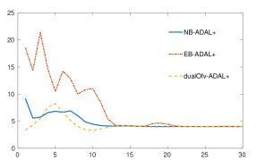
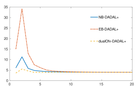
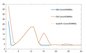
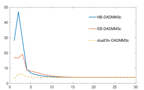
Figure 1: Evolution of the computed bounds on the instance johnson8_2_4.

5.4 Computational Setup

In our numerical experiments we compare the performance of ADAL+, DADAL+, ConicADMM3c and DADMM3c on $66$ instances of the DNN (20) to compute $\vartheta_{+}(G)$. The graphs are taken from the second DIMACS implementation challenge [8]. Note that in that challenge the task was to find a maximum clique of several graphs, so we consider the complement graphs of the graphs in [8]. In Table 2, for each instance on a graph $G$, we report its name (Problem) and its dimension (the number of vertices $n$ and the number of edges $m$ of $G$). The value of the Lovász theta function $\vartheta(G)$ for many of these instances can be found in [5] and [11], in this article we exclusively focus on $\vartheta_{+}(G)$.

Table 2: Data of the DIMACS instances considered in [8].

Problem	$n$	$m$	Problem	$n$	$m$	Problem	$n$	$m$
johnson8_2_4	28	168	hamming8_4	256	11776	p_hat500_2	500	61804
MANN_a9	45	72	p_hat300_1	300	33917	p_hat500_3	500	30950
hamming6_2	64	192	p_hat300_2	300	22922	p_hat700_1	700	183651
hamming6_4	64	1312	p_hat300_3	300	11460	p_hat700_2	700	122922
johnson8_4_4	70	560	MANN_a27	378	702	p_hat700_3	700	61640
johnson16_2_4	120	1680	brock400_1	400	20077	keller5	776	74710
keller4	171	5100	brock400_2	400	20014	brock800_1	800	112095
brock200_1	200	5066	brock400_3	400	20119	brock800_2	800	111434
brock200_2	200	10024	brock400_4	400	20035	brock800_3	800	112267
brock200_3	200	7852	san400_0_5_1	400	39900	brock800_4	800	111957
brock200_4	200	6811	san400_0_7_1	400	23940	p_hat1000_1	1000	377247
c_fat200_1	200	18366	san400_0_7_2	400	23940	p_hat1000_2	1000	254701
c_fat200_2	200	16665	san400_0_7_3	400	23940	p_hat1000_3	1000	127754
c_fat200_5	200	11427	san400_0_9_1	400	7980	san1000	1000	249000
san200_0_7_1	200	5970	sanr400_0_5	400	39816	hamming10_2	1024	5120
san200_0_7_2	200	5970	sanr400_0_7	400	23931	hamming10_4	1024	89600
san200_0_9_1	200	1990	johnson32_2_4	496	14880	MANN_a45	1035	1980
san200_0_9_2	200	1990	c_fat500_10	500	78123	p_hat1500_1	1500	839327
san200_0_9_3	200	1990	c_fat500_1	500	120291	p_hat1500_2	1500	555290
san200_0_7	200	6032	c_fat500_2	500	115611	p_hat1500_3	1500	277006
san200_0_9	200	2037	c_fat500_5	500	101559	MANN_a81	3321	6480
hamming8_2	256	1024	p_hat500_1	500	93181	keller6	3361	1026582

We implemented the four algorithms detailed in Sections 2 and 3 in MATLAB R2019a. In all computations, we set the accuracy level $\varepsilon$ to $10^{-5}$ and we set a time limit of $3600$ seconds CPU time. In both DADAL+ and DADMM3c we perform two iterations of Algorithm 3 in order to update $(y,V)$.

It is known that the performance of ADMMs strongly depends on the update of the penalty parameter $\sigma$. In all implementations, we use the strategy described by Lorenz and Tran-Dinh [10], so in iteration $k$ we set

$$\sigma^{k}=\frac{\lVert X^{k}\rVert}{\lVert Z^{k}\rVert}.$$

The experiments were carried out on an Intel Core i7 processor running at 3.1 GHz under Linux.

5.5 Comparison between ADAL+ and DADAL+

In Table LABEL:tab:ADAL+ we report the results obtained with ADAL+ and DADAL+ on the $66$ instances of computing $\vartheta_{+}(G)$ detailed in Table 2. We include the following data for the comparison: For each instance, we report its name (Problem) and its stability number ($\alpha$) and for each of the two algorithms, we report the dual objective function value obtained (d ofv), the bound obtained by computing the error bound described in Section 4.1 ($EB$), the bound obtained by applying the Nightjet procedure described in Section 4.2 ($NB$), the number of iterations (it) and the CPU time needed to satisfy the stopping criterion (time).

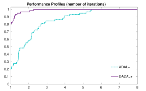
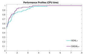
Figure 2: Comparison between ADAL+ and DADAL+ on DIMACS instances [8].

As a further comparison, we report in Figure 2 the performance profiles of ADAL+ and DADAL+ with respect to the number of iterations and the CPU time. These performance profiles are obtained in the following way. Given our set of solvers $\mathcal{S}$ and a set of problems $\mathcal{P}$, we compare the performance of a solver $s\in\mathcal{S}$ on problem $p\in\mathcal{P}$ against the best performance obtained by any solver in $\mathcal{S}$ on the same problem. To this end we define the performance ratio $r_{p,s}=t_{p,s}/\min\{t_{p,s^{\prime}}\mid s^{\prime}\in\mathcal{S}\},$ where $t_{p,s}$ is the measure we want to compare, and we consider a cumulative distribution function $\rho_{s}(\tau)=|\{p\in\mathcal{P}\mid r_{p,s}\leq\tau\}|/|\mathcal{P}|$. The performance profile for $s\in S$ is the plot of the function $\rho_{s}$.

Note that both ADAL+ and DADAL+ stopped on $7$ instances because of the time limit. In the performance profiles, we exclude those instances where at least one of the solvers exceeds the time limit.

It is clear from the results on Table LABEL:tab:ADAL+ and from the performance profiles that DADAL+ performs much less iterations than ADAL+. However, this does not always correspond to an improvement in terms of computational time as the double update of $y$ is an expensive operation.

With respect to the CPU time, Figure 2 shows that the performance of the two algorithms is similar, even if DADAL+ slightly outperforms ADAL+ as its curve is always above the other one.

If we consider the dual objective function value in Table LABEL:tab:ADAL+ we see that in fact the dual objective function value obtained by ADAL+ and DADAL+ is often not a bound, for example on the instances hamming6_4, c_fat200_1, san200_0_7_1, san400_0_9_1, c_fat500_1 and c_fat500_5. This shows that a procedure for obtaining a bound from the approximate solution is indeed of major importance.

Regarding the quality of the bounds, the Nightjet procedure is able to obtain better bounds with respect to the error bounds, both when applied as post-processing phase for ADAL+ and for DADAL+, for the vast majority of the instances. The improvement is particularly impressive when looking at those instances where the time limit is exceeded. We want to further highlight that the bound obtained from the Nightjet procedure comes from a newly computed feasible dual solution. This means that applying the Nightjet procedure as post-processing does not only guarantee a bound generally better than the one obtained by the error bounds, but it also provides a dual feasible solution.

Table 3: Comparison between ADAL+ and DADAL+ on DIMACS instances [8].

	ADAL+					DADAL+
Problem	d ofv	$EB$	$NB$	it	time	d ofv	$EB$	$NB$	it	time	$\alpha$
johnson8_2_4	3.99999	4.00037	4.00012	44	1.1	4.00000	4.00025	4.00009	25	0.5	4
MANN_a9	17.4750	17.4756	17.4755	765	1.1	17.4750	17.4756	17.4755	510	0.9	16
hamming6_2	32.0005	32.0005	32.0004	669	1.9	31.9996	32.0004	32.0000	250	1.0	32
hamming6_4	3.99994	4.00197	4.00016	56	0.1	3.99998	4.00110	4.00010	26	0.1	4
johnson8_4_4	13.9998	14.0016	14.0002	135	0.3	14.0001	14.0001	14.0004	47	0.3	14
johnson16_2_4	8.00000	8.00166	8.00034	89	0.6	8.00000	8.00411	8.00037	35	0.3	8
keller4	13.4659	13.4701	13.4667	764	8.7	13.4659	13.4716	13.4669	260	5.2	11
brock200_1	27.1968	27.2003	27.1978	312	4.9	27.1966	27.2002	27.2007	222	7.2	21
brock200_2	14.1310	14.1367	14.1325	158	2.6	14.1310	14.1359	14.1335	150	5.0	12
brock200_3	18.6718	18.6764	18.6727	219	3.5	18.6718	18.6764	18.6745	146	3.8	15
brock200_4	21.1211	21.1253	21.1220	264	4.2	21.1210	21.1254	21.1246	185	4.8	17
c_fat200_1	11.9999	12.0008	12.0006	339	5.2	11.9999	12.0009	12.0002	133	3.7	12
c_fat200_2	23.9981	24.0000	24.0000	2686	44.3	24.0015	24.0015	24.0014	782	21.9	24
c_fat200_5	60.3443	60.3483	60.3456	1218	19.1	60.3452	60.3474	60.3465	681	18.1	58
san200_0_7_1	29.9980	30.0000	30.0000	3441	54.6	29.9986	30.0000	30.0000	809	21.6	30
san200_0_7_2	18.0019	18.0019	18.0019	8782	144.6	18.0014	18.0014	18.0015	7614	202.6	18
san200_0_9_1	69.9980	70.0000	70.0000	3668	56.3	70.0009	70.0009	70.0008	670	16.1	70
san200_0_9_2	60.0020	60.0020	60.0019	3551	53.9	59.9991	60.0000	60.0000	688	17.0	60
san200_0_9_3	44.0016	44.0016	44.0016	11792	190.9	44.0010	44.0010	44.0014	10386	263.0	44
san200_0_7	23.6333	23.6372	23.6344	313	4.8	23.6332	23.6370	23.6364	218	5.9	18
san200_0_9	48.9046	48.9077	48.9063	403	6.1	48.9044	48.9070	48.9083	400	10.0	42
hamming8_2	128.002	128.002	128.002	2760	83.8	128.001	128.001	128.001	694	29.6	128
hamming8_4	16.0002	16.0002	16.0012	121	3.6	16.0001	16.0001	16.0011	52	3.0	16
p_hat300_1	10.0203	10.0348	10.0232	380	15.6	10.0202	10.0372	10.0208	457	30.3	8
p_hat300_2	26.7143	26.7154	26.7153	2315	94.2	26.7138	26.7274	26.7157	3576	230.0	25
p_hat300_3	40.7008	40.7096	40.7030	604	24.6	40.7003	40.7075	40.7061	817	51.1	36
MANN_a27	132.762	132.765	132.763	2037	136.4	132.762	132.766	132.765	768	77.9	126
brock400_1	39.3307	39.3438	39.3377	215	16.7	39.3308	39.3433	39.3391	148	18.5	27
brock400_2	39.1963	39.2083	39.2024	216	16.7	39.1964	39.2080	39.2037	152	19.0	29
brock400_3	39.1602	39.1742	39.1673	211	16.5	39.1603	39.1724	39.1679	149	19.2	31
brock400_4	39.2313	39.2455	39.2361	208	15.6	39.2313	39.2440	39.2363	146	18.3	33
san400_0_5_1	13.0038	13.0038	13.0036	8135	629.4	13.0034	13.0034	13.0032	4705	528.4	13
san400_0_7_1	39.9962	40.0000	40.0000	6654	516.5	40.0038	40.0038	40.0037	1723	213.6	40
san400_0_7_2	30.0037	30.0037	30.0036	7999	623.3	30.0032	30.0032	30.0031	3863	468.0	30
san400_0_7_3	22.0000	22.0084	22.0044	601	47.9	22.0002	22.0143	22.0010	265	31.1	22
san400_0_9_1	99.9960	100.000	100.000	7212	547.5	99.9978	100.000	100.000	1499	167.8	100
sanr400_0_5	20.1782	20.1924	20.1794	164	12.6	20.1782	20.1924	20.1839	115	15.2	13
sanr400_0_7	33.9666	33.9794	33.9727	186	14.5	33.9666	33.9790	33.9724	141	17.3	21
johnson32_2_4	15.9999	16.0047	16.0000	272	36.8	16.0000	16.0264	16.0005	69	12.4	16
c_fat500_10	126.003	126.003	126.003	3752	509.8	126.000	126.001	126.001	2772	549.4	126
c_fat500_1	13.9992	14.0113	14.0015	488	64.7	13.9987	14.0147	14.0004	251	58.9	14
c_fat500_2	25.9988	26.0136	26.0007	554	74.7	25.9990	26.0116	26.0003	302	69.8	26
c_fat500_5	63.9970	64.0040	64.0008	2740	374.1	63.9969	64.0044	64.0007	1104	252.4	64
p_hat500_1	13.0080	13.0401	13.0102	342	46.4	13.0079	13.0454	13.0088	380	81.0	9
p_hat500_2	38.5606	38.5638	38.5653	2159	290.5	38.5594	38.5871	38.5619	4404	907.9	36
p_hat500_3	57.8122	57.8287	57.8220	850	117.5	57.8111	57.8251	57.8155	1021	208.3	$\geq 50$
p_hat700_1	15.0452	15.0996	15.0500	361	117.4	15.0451	15.1077	15.0460	422	204.8	11
p_hat700_2	48.4420	48.4466	48.4463	2168	696.3	48.4401	48.4827	48.4436	4901	2388.1	44
p_hat700_3	71.7569	71.7761	71.7701	1234	391.6	71.7551	71.7853	71.7736	1543	727.0	62
keller5	30.9956	31.0461	30.9987	1684	767.0	30.9956	31.0469	30.9984	1970	1136.6	27
brock800_1	41.8673	41.9080	41.8712	232	118.6	41.8673	41.9107	41.8701	107	81.8	23
brock800_2	42.1043	42.1446	42.1071	231	121.6	42.1043	42.1477	42.1067	107	80.1	24
brock800_3	41.8825	41.9235	41.8860	234	125.4	41.8825	41.9251	41.8859	109	84.9	25
brock800_4	42.0006	42.0426	42.0037	232	122.9	42.0006	42.0429	42.0034	108	84.1	26
p_hat1000_1	17.5225	17.5888	17.5303	475	660.2	17.5222	17.6307	17.5233	492	872.0	$\geq 10$
p_hat1000_2	54.8464	54.8586	54.8522	1919	2583.9	54.8440	55.0811	54.8723	2013	$\geq 3600$	$\geq 46$
p_hat1000_3	83.5297	83.5515	83.5469	1457	1954.8	83.5285	83.5677	83.5367	1403	2460.7	$\geq 68$
san1000	15.0003	15.1126	15.0016	1757	2420.4	14.9999	15.0527	15.0282	893	1538.7	15
hamming10_2	5819.50	5819.50	5809.20	2141	$\geq 3600$	512.220	512.220	512.220	1919	$\geq 3600$	512
hamming10_4	42.6673	42.6755	42.6678	576	947.2	42.6670	42.7206	42.6674	107	198.9	40
MANN_a45	14869.8	14869.8	14869.8	2289	$\geq 3600$	356.048	356.070	356.055	873	1670.5	345
p_hat1500_1	21.8947	22.0632	21.9062	563	$\geq 3600$	21.8925	22.6598	21.8976	486	$\geq 3600$	12
p_hat1500_2	75.9170	84.6770	89.5774	562	$\geq 3600$	76.4810	76.6852	76.6293	479	$\geq 3600$	65
p_hat1500_3	303.073	374.111	342.539	562	$\geq 3600$	113.701	113.981	113.779	491	$\geq 3600$	94
MANN_a81	859.136	2131.14	1467.70	50	$\geq 3600$	4127.67	4127.80	4127.67	45	$\geq 3600$	1100
keller6	3655.24	3661.45	3637.22	47	$\geq 3600$	97.8409	322.341	103.789	43	$\geq 3600$	$\geq 59$

5.6 Comparison between ConicADMM3c and DADMM3c

In Table LABEL:tab:ConicDADMM3c we report the results obtained with ConicADMM3c and DADMM3c on the $66$ instances of computing $\vartheta_{+}(G)$ detailed in Table 2.

As before, we report the name of the instances, the stability number and, for each algorithm, the dual objective function value obtained, the bounds obtained by computing the error bound and by applying the Nightjet procedure, the number of iterations and the CPU time needed to satisfy the stopping criterion.

ConicADMM3c was not able to stop within the time limit on $11$ instances, while DADMM3c was not able to stop within the time limit on $15$ instances.

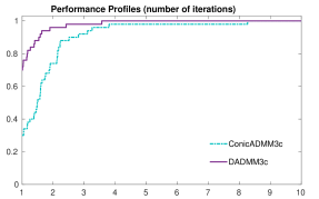
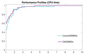
Figure 3: Comparison between ConicADMM3c and DADMM3c on DIMACS instances [8].

In general, DADMM3c needs to perform much less iterations and it is slightly better than ConicADMM3c in terms of CPU time as it is confirmed by the performance profiles shown in Figure 3. As before, we did not include the instances that exceeded time limit in the performance profiles.

Again, the Nightjet procedure is able to obtain better bounds with respect to the error bounds, both when applied as post-processing phase for ConicADMM3c and for DADMM3c, for the majority of the instances. However, there exist cases ($6$ instances) where the Nightjet procedure fails.

We finally mention that on several instances where the time limit was exceeded, the bounds obtained by DADMM3c are much better than those obtained by ConicADMM3c, see for example the instances p_hat1500_1, p_hat1500_2 and p_hat1500_3.

Table 4: Comparison between ConicADMM3c and DADMM3c on DIMACS instances [8].

	ConicADMM3c					DADMM3c
Problem	d ofv	$EB$	$NB$	it	time	d ofv	$EB$	$NB$	it	time	$\alpha$
johnson8_2_4	3.99997	4.00033	4.00000	53	0.1	4.00000	4.00017	4.00010	28	0.1	4
MANN_a9	17.4752	17.4752	17.4752	277	0.5	17.4750	17.4756	17.4755	988	4.4	16
hamming6_2	31.9996	32.0004	32.0000	776	2.6	32.0001	32.0001	32.0001	309	2.3	32
hamming6_4	4.00002	4.00025	4.00002	69	0.2	4.00000	4.00145	4.00020	50	0.3	4
johnson8_4_4	13.9999	14.0013	14.0002	151	0.5	14.0000	14.0000	14.0007	286	2.4	14
johnson16_2_4	7.99995	8.00133	8.00000	106	1.0	8.00000	8.00404	8.00044	66	0.9	8
keller4	13.4660	13.4711	13.4670	338	7.1	13.4659	13.4703	13.4660	552	16.9	11
brock200_1	27.1967	27.2002	27.2004	332	9.6	27.1967	27.2020	27.1982	317	12.9	21
brock200_2	14.1310	14.1371	14.1324	199	5.9	14.1310	14.1380	14.1320	231	10.5	12
brock200_3	18.6718	18.6771	18.6734	226	6.8	18.6718	18.6778	18.6729	286	12.2	15
brock200_4	21.1210	21.1257	21.1248	260	8.4	21.1211	21.1269	21.1223	222	9.8	17
c_fat200_1	11.9999	12.0025	12.0004	261	8.6	12.0001	12.0004	12.0004	165	7.8	12
c_fat200_2	24.0017	24.0017	24.0017	1686	54.2	23.9981	24.0000	24.0002	974	45.3	24
c_fat200_5	60.3461	60.3461	60.3461	1469	45.0	60.3444	60.3481	60.3463	996	46.2	58
san200_0_7_1	30.0019	30.0019	30.0019	2039	65.6	30.0019	30.0022	30.0019	1161	47.7	30
san200_0_7_2	17.9991	18.0001	18.0012	8265	246.6	17.9421	18.0121	18.0131	87753	$\geq 3600$	18
san200_0_9_1	70.0019	70.0019	70.0019	2472	77.8	69.9980	70.0000	70.0001	1113	40.9	70
san200_0_9_2	60.0017	60.0017	60.0017	2340	74.3	59.9980	60.0000	60.0001	1098	40.7	60
san200_0_9_3	43.9983	44.0000	44.0000	11443	342.1	43.9984	44.0005	44.0002	10892	401.7	44
san200_0_7	23.6332	23.6370	23.6364	311	9.7	23.6333	23.6390	23.6347	323	12.1	18
san200_0_9	48.9044	48.9070	48.9084	686	21.5	48.9046	48.9049	48.9050	1659	61.1	42
hamming8_2	127.998	128.002	128.000	4163	245.5	11.9202	434.728	Inf	52831	$\geq 3600$	128
hamming8_4	15.9997	16.0119	16.0006	168	9.8	15.9998	16.0087	15.9999	266	18.5	16
p_hat300_1	10.0203	10.0356	10.0213	404	31.6	10.0203	10.0339	10.0211	463	46.3	8
p_hat300_2	26.7141	26.7146	26.7142	3425	261.5	26.7167	26.7233	26.7197	1102	107.2	25
p_hat300_3	40.7008	40.7098	40.7032	822	63.7	40.7012	40.7092	40.7043	832	77.5	36
MANN_a27	132.762	132.765	132.763	7179	914.3	26.9452	487.963	Inf	22536	$\geq 3600$	126
brock400_1	39.3308	39.3434	39.3381	528	80.7	39.3309	39.3455	39.3331	331	61.1	27
brock400_2	39.1964	39.2079	39.2024	532	79.9	39.1965	39.2113	39.1987	367	67.4	29
brock400_3	39.1602	39.1734	39.1675	526	81.4	39.1604	39.1749	39.1628	335	61.7	31
brock400_4	39.2313	39.2446	39.2361	515	78.6	39.2314	39.2459	39.2339	370	69.3	33
san400_0_5_1	13.0015	13.0015	13.0015	5691	853.4	13.0035	13.0056	13.0035	5878	1152.4	13
san400_0_7_1	39.9966	40.0000	40.0000	3961	601.7	39.9961	40.0000	40.0001	2663	498.9	40
san400_0_7_2	29.9991	30.0000	30.0004	6704	996.0	29.9967	30.0020	30.0000	4459	823.8	30
san400_0_7_3	22.0000	22.0063	22.0009	962	147.5	22.0000	22.0110	22.0015	253	46.1	22
san400_0_9_1	100.003	100.003	100.003	4803	719.6	99.9961	100.000	100.000	2520	440.6	100
sanr400_0_5	20.1782	20.1934	20.1837	282	42.6	20.1782	20.1975	20.1797	332	66.4	13
sanr400_0_7	33.9666	33.9790	33.9726	434	66.1	33.9666	33.9825	33.9685	347	63.2	21
johnson32_2_4	16.0000	16.0000	16.0000	769	194.9	16.0000	16.0309	16.0006	93	29.0	16
c_fat500_10	125.997	126.003	126.002	6666	1729.1	168.342	170.112	168.580	10895	$\geq 3600$	126
c_fat500_1	13.9997	14.0050	14.0007	478	132.3	13.9995	14.0063	14.0005	300	103.5	14
c_fat500_2	26.0000	26.0034	26.0012	717	192.3	25.9994	26.0076	26.0009	384	134.7	26
c_fat500_5	63.9975	64.0029	64.0020	3752	966.2	64.0027	64.0030	64.0027	1684	562.4	64
p_hat500_1	13.0081	13.0401	13.0103	449	118.6	13.0080	13.0383	13.0092	631	208.9	9
p_hat500_2	38.5599	38.5606	38.5600	4417	1138.1	38.5649	38.5767	38.5891	1356	437.8	36
p_hat500_3	57.8119	57.8307	57.8198	1312	340.3	57.8137	57.8320	57.8457	1128	349.1	$\geq 50$
p_hat700_1	15.0453	15.0996	15.0475	492	314.4	15.0454	15.0948	15.0504	756	593.9	11
p_hat700_2	48.4405	48.4416	48.4407	4971	3074.1	48.4470	48.4608	48.4739	1765	1355.9	44
p_hat700_3	71.7561	71.7819	71.7968	2256	1413.6	71.7635	71.7882	71.8177	1372	1018.2	62
keller5	30.9956	31.0441	30.9980	2301	1988.5	30.9957	31.0352	30.9958	3470	$\geq 3600$	27
brock800_1	41.8673	41.9094	41.8704	805	836.6	41.8674	41.9137	41.8675	370	436.4	23
brock800_2	42.1043	42.1456	42.1069	808	849.2	42.1043	42.1512	42.1044	382	449.6	24
brock800_3	41.8825	41.9255	41.8903	801	839.9	41.8826	41.9291	41.8826	374	443.5	25
brock800_4	42.0006	42.0433	42.0058	805	846.1	42.0006	42.0470	42.0007	375	444.1	26
p_hat1000_1	17.5223	17.5606	17.5261	773	2124.9	17.5226	17.6075	17.5242	1071	3400.0	$\geq 10$
p_hat1000_2	54.7944	55.5397	56.0385	1317	$\geq 3600$	54.8680	54.9231	54.9417	1168	$\geq 3600$	$\geq 46$
p_hat1000_3	7663.81	7663.82	7770.75	1327	$\geq 3600$	83.5456	83.5930	83.6149	1188	$\geq 3600$	$\geq 68$
san1000	81.8129	82.3795	84.5386	1282	$\geq 3600$	15.0315	15.1395	15.0506	1144	$\geq 3600$	15
hamming10_2	314167	314167	314167	1154	$\geq 3600$	65.1578	2179.24	Inf	1024	$\geq 3600$	512
hamming10_4	1653.80	1653.8	1653.80	1117	$\geq 3600$	42.6662	42.7279	42.6680	265	881.6	40
MANN_a45	181901	181901	181901	1159	$\geq 3600$	36.1173	1117.01	Inf	1061	$\geq 3600$	345
p_hat1500_1	2850.61	2850.61	2850.61	280	$\geq 3600$	22.0204	22.6797	22.0222	262	$\geq 3600$	12
p_hat1500_2	21212.1	21212.1	21212.1	280	$\geq 3600$	76.7168	78.3033	76.7352	268	$\geq 3600$	65
p_hat1500_3	41630.4	41630.4	41630.4	282	$\geq 3600$	114.243	116.135	114.301	271	$\geq 3600$	94
MANN_a81	388.942	3282.73	2205.46	25	$\geq 3600$	93.4902	3269.63	Inf	24	$\geq 3600$	1100
keller6	1902.86	1902.86	Inf	22	$\geq 3600$	181.517	184.845	197.191	24	$\geq 3600$	$\geq 59$

6 Conclusions

In this paper we propose to use a factorization of the dual matrix within two ADMMs for conic programming proposed in the literature. In particular we use a first order update of the dual variables in order to improve the performance of the ADMMs considered.

Our computational results on instances from a DNN relaxation of the stable set problem show that the factorization employed gives a significant improvement in the efficiency of the methods. We are confident that this can be the case also when dealing with other structured DNNs. In particular, we experience a drastic reduction in terms of number of iterations. The performance of DADMM3c may even further improve through a smart update of the rank of $Z$ along the iterations. This is a topic for future investigation.

In the paper we also focus on how to obtain bounds on the primal optimal objective function value, since the dual objective function value obtained when using first order methods to solve DNNs is not always guaranteed to serve as bound, as the dual solution may be infeasible. We present two methods: one that adds a sufficient (negative) perturbation to the dual objective function value (error bounds) and one that constructs a dual feasible solution (Nightjet procedure). Both methods are computationally cheap and produce bounds close to the optimal objective function value of the DNN if the obtained solution is close to the optimal solution. The Nightjet procedure works particularly well for structured instances, like computing $\vartheta_{+}$, but comes with the drawback that it might fail to produce a feasible solution. However, as long as the dual solution is reasonably close to the (unknown) optimal solution, this does not happen. We also observe that the Nightjet procedure works particularly well after ADAL+ and DADAL+. This is due to the fact that in these algorithms the dual matrix (which is the input for the Nightjet procedure) is positive semidefinite by construction. The two versions of the post-processing make our methods applicable within branch-and-bound frameworks in order to solve combinatorial optimization problems with DNN relaxations.

Our plan for future research is to apply the methods to other structured DNN relaxations. Furthermore, we will expand our methods to solve SDPs with general inequality constraints instead of just nonnegativity.

References

- [1] Dimitri P. Bertsekas. Constrained optimization and Lagrange multiplier methods. Computer Science and Applied Mathematics. Academic Press Inc., New York, 1982.
- [2] Caihua Chen, Bingsheng He, Yinyu Ye, and Xiaoming Yuan. The direct extension of ADMM for multi-block convex minimization problems is not necessarily convergent. Mathematical Programming, 155(1-2):57–79, 2016.
- [3] Marianna De Santis, Franz Rendl, and Angelika Wiegele. Using a factored dual in augmented Lagrangian methods for semidefinite programming. Operations Research Letters, 46(5):523 – 528, 2018.
- [4] Elisabeth Gaar and Franz Rendl. A bundle approach for SDPs with exact subgraph constraints. In Andrea Lodi and Viswanath Nagarajan, editors, Integer Programming and Combinatorial Optimization, pages 205–218. Springer International Publishing, 2019.
- [5] Monia Giandomenico, Adam N. Letchford, Fabrizio Rossi, and Stefano Smriglio. Approximating the Lovász function with the subgradient method. Electronic Notes in Discrete Mathematics, 41:157 – 164, 2013.
- [6] Johan Håstad. Clique is hard to approximate within . Acta Mathematica, 182(1):105–142, 1999.
- [7] Christian Jansson, Denis Chaykin, and Christian Keil. Rigorous error bounds for the optimal value in semidefinite programming. SIAM Journal on Numerical Analysis, 46(1):180–200, 2007/08.
- [8] David J. Johnson and Michael A. Trick, editors. Cliques, Coloring, and Satisfiability: Second DIMACS Implementation Challenge, Workshop, October 11-13, 1993. American Mathematical Society, 1996.
- [9] Richard M. Karp. Reducibility among combinatorial problems. In Raymond E. Miller, James W. Thatcher, and Jean D. Bohlinger, editors, Complexity of Computer Computations, The IBM Research Symposia Series, pages 85–103. Springer US, 1972.
- [10] Dirk A. Lorenz and Quoc Tran-Dinh. Non-stationary Douglas–Rachford and alternating direction method of multipliers: adaptive step-sizes and convergence. Computational Optimization and Applications, 74(1):67–92, Sep 2019.
- [11] Jérôme Malick, Janez Povh, Franz Rendl, and Angelika Wiegele. Regularization methods for semidefinite programming. SIAM J. Optim., 20(1):336–356, 2009.
- [12] Franz Rendl. Matrix relaxations in combinatorial optimization. In Jon Lee and Sven Leyffer, editors, Mixed Integer Nonlinear Programming, pages 483–511. Springer New York, 2012.
- [13] Alexander Schrijver. A comparison of the Delsarte and Lovász bounds. IEEE Transactions on Information Theory, 25(4):425–429, 1979.
- [14] Defeng Sun, Kim-Chuan Toh, and Liuqin Yang. A convergent 3-block semiproximal alternating direction method of multipliers for conic programming with 4-type constraints. SIAM Journal on Optimization, 25:882–915, 2015.
- [15] Zaiwen Wen, Donald Goldfarb, and Wotao Yin. Alternating direction augmented Lagrangian methods for semidefinite programming. Mathematical Programming Computation, 2(3):203–230, 2010.