Knotted 3-balls in
Abstract.
The unknot in has non-unique smooth spanning -balls up to isotopy fixing . Equivalently there are properly embedded non-separating 3-balls in not properly isotopic to . More generally there exist non-separating 3-spheres in not isotopic to and non trivial elements of . Along the way we introduce barbell diffeomorphisms, implantations and twistings to construct and modify diffeomorphisms homotopic to the identity. We also introduce a 2-parameter calculus of embeddings of the interval into 4-manifolds and introduce a framed cobordism method as well as a direct method for showing that certain 2-parameter families are homotopically non trivial and diffeomorphisms are isotopically nontrivial. Extensions to higher dimensional manifolds are obtained.
Primary class: 57M99
secondary class: 57R52, 57R50, 57N50
keywords: 4-manifolds, 2-knots, isotopy
1. Introduction
This paper introduces the study of knotted 3-balls in 4-manifolds, in particular the 4-sphere and . Let be the unit sphere in . Define a standard -ball in to be a great 3-ball, i.e. a geodesic 3-ball with boundary a great 2-sphere. A knotted ball in means a smoothly-embedded -ball whose boundary is a great -sphere which is not isotopic keeping the boundary fixed, to a standard 3-ball . The requirement that the boundary be constrained throughout the isotopy is necessary since any two embedded -balls in the interior of a connected -manifold are ambiently isotopic [Ce1] p. 231, [Pa]. The existence of knotted 3-balls in contrasts with the uniqueness of spanning discs for the unknot in and uniqueness for spanning discs for circles in , [Ga1]. This paper works in the smooth category and unless otherwise said, all mappings are smooth.
We say is a reducing -ball in if is a properly-embedded submanifold, diffeomorphic to such that the complement is connected. By properly-embedded we mean that . A reducing -ball is knotted if it is not properly isotopic to the linear reducing -ball, . All reducing -balls are properly homotopic to . The study of reducing 3-balls up to isotopy is equivalent to the study of such balls that coincide with near the boundary since Allen Hatcher has proven that the space of non-separating embeddings of in has the homotopy-type of [Ha2].
Isotopy classes of reducing -balls in admit an abelian group structure coming from an operation similar to boundary connect-sum, that we call concatenation defined as follows. Starting with two reducing -balls in whose boundary is , one glues the two copies of together along where is a hemisphere in . This produces a new -manifold canonically diffeomorphic to together with a new reducing -ball. We will see in Sections 3 and 9 that concatenation has inverses, i.e. it is a group, with the unit being the linear reducing sphere. A less abstract way to describe concatenation would be to take and assume are disjoint -balls. One can assume provided and otherwise. Define the sum of and to be equal to on where . Isotopy classes of oriented 3-balls in where the embeddings are required to be linear on the boundary also have a group structure, defined in essentially the same way, and these groups are isomorphic. The key point is that the closed complement (the exterior) of the unknotted in is diffeomorphic to .
We use the convention that if is a manifold with boundary, then denotes the diffeomorphisms of that are the identity on the boundary. Similarly, we use the notation to denote the subgroup of diffeomorphisms homotopic to the identity. We shall see in §3 and §9 that the diffeomorphism groups , and are abelian and act transitively respectively on 3-balls with common boundary, reducing balls with common boundary and reducing 3-spheres. (Actually, is a -fold loop space compatible with the group multiplication [Bu1].) This leads to the theorem and equivalently the closed complement of the unknot in , have up to isotopy, infinitely many distinct fiberings over as does .
A diffeomorphism properly homotopic to the identity, gives rise to the 3-ball which is unknotted if and only if is properly isotopic to a map supported in a 4-ball. The group of isotopy classes of oriented 3-balls that are linear on their boundary is isomorphic to . Similarly, is isomorphic to the group of reducing 3-spheres in . See Theorem 3.13 and Theorem 3.12.
The main result of this paper is a construction of an infinite family of linearly independent elements of with explicit constructions of the corresponding knotted 3-balls in and hence . Furthermore, these diffeormorphisms extend to a linearly independent set in . The techniques of this paper also construct subgroups of whenever .
Denote the component of the unknot in by . A consequence of the above results is that does not have the homotopy type of the subspace of linear embeddings. The latter has the homotopy type of the Stiefel manifold while the former has a non-finitely-generated fundamental group. See Theorem 10.1.
We give a framework for approaching the smooth -dimensional Schönflies problem, describing the set of counter-examples as the fixed points of an endomorphism The endomorphism is given by lifting such an embedding to a non-trivial finite-sheeted covering space of . The non-trivial elements of we construct in this paper all belong to the kernel of iterates of this endomorphism.
The paper is organized as follows. In Section §2 we compute the homotopy group and show that it contains an infinitely-generated free abelian group provided , giving explicit generators , . This result extends the work of Dax [Da] who among other things computed in terms of certain cobordism groups and Arone-Szymik [AS], who show and of contain infinitely-generated free abelian groups. For we describe other generators in terms of embeddings of tori . In §3 we compute the three and five dimensional rational homotopy groups of and use them to define the invariant of which takes values in a quotient of . We define a 2-parameter family of and show that is equal to the class of the standard Whitehead product . We also describe fibration sequences relating various embedding spaces and diffeomorphism groups and also show that and respectively act transitively on reducing balls and spheres. In §4 we introduce geometric methods for working with 2-parameter families of . In particular, we introduce a bracket operation that produces a 2-parameter family from two 1-parameter families that are null homotopic and have disjoint domain and range supports. In §5 we introduce the barbell map of which we call the barbell neighborhood . fixes pointwise hence induces homotopically trivial diffeomorphisms of 4-manifolds called implantations when is embedded in a 4-manifold and is pushed forward. We describe the implantations of induced from the generating elements . We also compute of the standard separating 3-ball . This is used in §6 to produce two parameter families in arising from the ’s. We then show how to modify these families when twisting the implantation. In §7 we compute the class as the sum of elements of a -matrix with entries a sum of ’s. This matrix is skew symmetric and hence . In §8 we show that the effect of twisting the implantation is to modify by row and column operations. By twisting the implantations we produce the implantations, , whose homotopy classes are shown to be linearly independent by the invariant. Together with the triviality of the ’s we conclude that the implantations in are linearly independent up to isotopy. In §9 we discuss the relation between knotted 3-balls and the smooth 4-dimensional Schoenflies conjecture. More applications are given in §10 and questions and conjectures are given in §11. In the Appendix we give a direct argument that is equivalent to the standard Whitehead product up to sign independent of and .
Independently, Tadayuki Watanabe [Wa2] has constructed an invariant
and has shown it to be non-trivial on some diffeomorphisms created via his graph surgery construction.
Acknowledgements. The authors would like to thank the Banff International Research Station. The Unifying 4-Dimensional Knot Theory meeting at BIRS was crucial to this project. The authors would also like to thank Greg Arone and Markus Szymik for helpful discussions. The authors also thank Allen Hatcher, Tadayuki Watanabe and François Laudenbach for helpful comments on the initial version of the paper. The first author thanks BIRS for hosting the Spaces of Embeddings: Connections and Applications meeting in the fall of 2019, where some useful developments occurred for this paper. He also thanks Dev Sinha for helpful discussions, and Alan Mehlenbacher for pointing out mistakes in early drafts of this paper. The second author’s work on this project was initiated during visits to Trinity College, Dublin and work was also carried out while visiting the Max Planck Institute for Mathematics, Bonn and the Mathematical Institute at Oxford University. He thanks all these institutions for their hospitality. He thanks Toby Colding for long conversations years ago and Maggie Miller for recent helpful conversations. Special thanks to Martin Bridgeman. He was partially supported by NSF grants DMS-1607374 and DMS-2003892.
2. Embeddings of circles in
In this section we describe a range of low-dimensional homotopy groups of . These results were essentially known to Dax [Da], who used a Haefliger-style parametrized double-point elimination process to describe the low-dimensional homotopy groups of a variety of embedding spaces. Given an element of an embedding space we will denote the path-component of containing by .
We begin with the least technical elements in Theorem 2.5, describing for , three epimorphisms:
The epimorphisms and are defined for all components of the embedding space. The group is defined as a quotient of the Laurent polynomial ring , and contains a free abelian subgroup of infinite rank. It can also contain -torsion.
For this definition we consider the Laurent polynomial ring to be only a group. We define to be the quotient group, modulo the subgroup generated by the relations
The group is the free abelian group on the generators
with the sole exception when is even, and is odd. In this case one has the same generating set , but represents -torsion. The remaining are free generators, i.e. .
The definitions of the maps and will be elementary applications of basic transversality theory.
Definition 2.1.
Let be defined as . Given an embedding , define . This is the degree of the map .
The value only depends on the homotopy class of . Provided , the homotopy class of agrees with the isotopy class, by transversality. Thus
is a bijection. An embedding satisfying would have .
Definition 2.2.
Given we define
where is defined as , i.e. we consider and we evaluate it at .
We can consider to be a function
As a thought experiment, argue that given satisfying , one can assume . More generally, one can show where is the subspace of where . From this perspective, is simply the induced map from the projection onto the first factor, i.e. .
An appealing way to think of the invariants and is via the inclusion , i.e. we are including the embedding space in the space of all continuous functions from to . Notice that and extend to invariants of and respectively. Moreover, as invariants of the homotopy-groups of they are isomorphisms, since splits as a direct product of two free loop spaces, . A simple general position argument tells us that the inclusion induces an epi-morphism on and an isomorphism on for . The rough idea is that if one has a map from a -dimensional manifold one constructs the track of the map given by . By transversality, this map can be uniformly approximated by a smooth embedding if , i.e. (see for example Theorem 2.13 [Hir]). Such an approximation is no longer a track-type function on the nose, but given that the approximation is uniform in (at least) the -topology, and the fact that diffeomorphisms of form an open subset of the space of maps , one can apply a diffeomorphism of (close to ) to generate an approximation that is the track of an embedding. The first two non-trivial homotopy-groups of are and , both infinite cyclic. The next non-trivial homotopy-group is .
The next invariant has the form
By the previous paragraph, it measures the lowest-dimensional deviation between the homotopy-types of and .
Definition 2.3.
Let denote the configuration space of pairs of distinct points in ,
Denote the cocircular pair subspace of by . The cocircular pair subspace is -dimensional, having co-dimension in . Given , assume the induced map
is transverse to , where . In such a situation we will associate .
Our polynomial will be akin to the transverse intersection number of with , but we include an enhancement into the definition. The set is invariant, and acts freely on . The invariant will be a sum of monomials associated to the points of . Given a point we associate an element and define
We define , where is the local oriented intersection number of with at . Observe the map
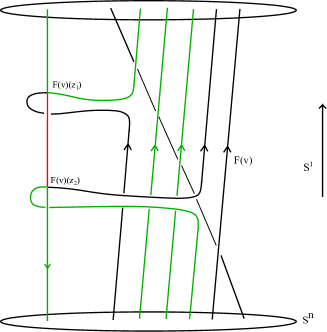
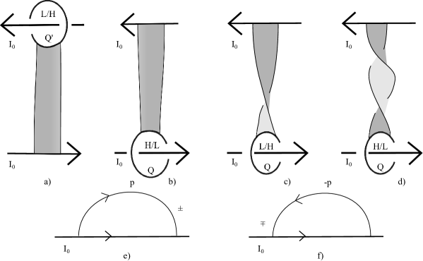
is a diffeomorphism between and . This is how we give its orientation. This map is also -equivariant. The monomial degree is computed via a pair of conventions. If , let denote the counter-clockwise oriented arc in that starts at and ends at . Similarly, given a point of , , the cocircular arc with this boundary is denoted . When thinking of we refer to this as the vertical orientation. The monomial degree is obtained by concatenating with the opposite-oriented cocircular arc in associated to , and taking the degree of the projection to the factor of . We depict an example in Figure 1, with the concatenation appearing in green. The unused portion of the vertical circle is in red. In this example , and .
 |
Notice that naturally factors as after projecting-out the factor, using the product decomposition .
Given then we also have and one can check
We use the notation to denote the -linear mapping satisfying . Thus is well-defined for . The relation in was chosen to ensure is a homotopy-invariant of . We use a compactification of configuration spaces to check homotopy-invariance.
Our manifold compactification of is diffeomorphic to an annulus . The boundary circles correspond to ‘infinitesimal’ configurations of pairs of points in ; one component where the direction vector from to agrees with the orientation of , and the other being the reverse.
The Fulton-MacPherson compactified configuration space has the rather simple model of blown up along its diagonal . Typically this is made formally precise by defining to be the closure of the graph of a function [Si2], such as where , assuming . This compactification is functorial under embeddings of manifolds. The inclusion is a homotopy-equivalence, i.e. is diffeomorphic to remove an open tubular neighbourhood of the diagonal . There is a canonically-defined onto smooth map , where the pre-image of is , which is canonically isomorphic to the unit tangent bundle of . The interior of is mapped diffeomorphicly to .
We now prove the homotopy-invariance of . Consider what happens in a homotopy of . The boundary of consists of the temporal part and the annular part . The only monomial degrees that run off the annular part of the boundary are . For example, runs off the annular part if in our transverse family we have a tangent vector to our knot pointing in the vertical direction, oriented counter-clockwise. Similarly, can run off the boundary if we produce a tangent vector in the vertical direction, oriented clockwise. The monomials and are symmetric, after re-labelling the points of the domain .
Thus if we consider to be an element of the quotient group , it is a homotopy-invariant.
Definition 2.4.
Let and define the half-ball . is a manifold with corners. As such, it is a stratified space with two co-dimension one strata, the round boundary and the flat boundary . These two boundaries meet at the corner (co-dimension two) stratum .
 |
Theorem 2.5.
Let . Provided both and are epimorphisms. When the map
is an epimorphism, i.e. is an epi-morphism.
Proof.
That is an epimorphism follows from the splitting , as it is the degree of the projection to the factor.
To argue that is an epimorphism, we start with the fixed degree near-linear embedding , depicted in black in Figure 2.
Imagine an immersed half-ball that is an embedding with the exception of a regular double point on the round boundary. We demand coincides with the flat boundary of . As in Figure 2 we demand that the map from the flat part of the boundary of to the vertical factor has no critical points. We further demand that the arc in connecting the double points projects to a degree map in the vertical factor, and that (as in Figure 2) the double-point occurs near the bottom of the flat boundary.
We modify the embedding , creating a new immersed curve by replacing the arc with , i.e. we cut out the flat boundary of from and replace it with the round boundary. This immersed curve is depicted in Figure 2 as the union of the solid black vertical broken curve (depicting with the flat boundary removed), with the solid red curve (depicting the round boundary of ). Call this immersed curve . Given that , we can assume the projection of to is also an immersion, and embedding at all but the single double point.
The sum of the tangent spaces at the double-point of is -dimensional, so the orthogonal complement is -dimensional, having an -parameter family of unit normal vectors. Using a bump function, given a unit normal vector one can perturb one strand of at the double-point, creating an embedded circle in . This gives us our family of resolutions,
The fact that the projection of to was an embedding with the sole exception of the single double-point allows us to conveniently identify the cocircular points in our family , giving us . ∎
We have an involution of that negates the invariant. One description is the process that sends the embedding to . Call this embedding . Then we have , i.e. the elements are symmetric about .
Another family to consider is one where is an embedding. We demand that intersects along the flat boundary, and also at a single point along the round boundary – a regular double point. Consider the case where the projection of the embedding to the factor is not onto, i.e. it is constrained to an interval in the factor. Then connects one strand of to adjacent strands. Let’s say to the -th strand (using the cyclic ordering) with , assuming . Call the resolved family of knots . Given that, we have . Recall that . Thus spans the same subspace of as the monomials , i.e. all the intermediate monomials that were not killed by the definining relations of .
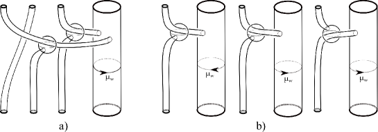
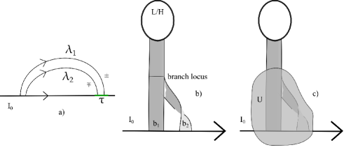
We give an alternative way to visualize elements of with by embedded tori, where denotes the standard generator of , i.e. the component. Each generator will be represented by an embedded torus which contains the curve . Such a torus gives rise to an element of by fibering by parametrized smooth circles with . Once is chosen, what really matters is which way to go around the torus. To do this and control , we choose an oriented simple closed curve , homotopically trivial in , that intersects transversely once at some point . The homotopy condition implies that that and the orientation informs us that is required to spin about so that follows in the oriented direction. Denote by the represented element of .
 |
| (a) | Vertical torus in . Vertical fibers represent trivial |
|---|---|
| element in , in the component with . | |
| (b) | Sphere linking tube in -space. |
The standard vertical torus , shown in Figure 3(a) represents the trivial element of . Figures 4 (a) and (b) describe embedded tori corresponding to and respectively. In our diagrams, , with being depicted horizontally as in Figure 3 (b). In a similar manner we obtain a torus corresponding to . Each of our tori is constructed by tubing with an unknotted, unlinked 2-sphere as follows. Emanating from the boundary of a small disc on the tube first links the sphere, then goes times around the factor before finally connecting to the 2-sphere. Figures 4 (a) and (b) show the projection of to where is identified with , where each component of is identified to a point. By construction , except for where the tube links the 2-sphere. See Figure 3(b) for a detail. The crossing convention for the tube and sphere informs us that the part of the tube that projects to the right side of the 2-sphere lives a bit in the past (i.e. in ) and the part of the tube on the left lives in the future. By construction, the 2-sphere bounds a 3-ball that intersects the tube is a single simple closed curve. By either reversing the way the tube links the 2-sphere, or reversing the orientation on we obtain the inverse of the generator. See Figure 6(b).
Proposition 2.6 relates the generators and , described above. To make this proposition precise, and not simply up to a choice of sign, we need to provide an orientation to the parametrizing sphere of our generators . The parametrizing sphere came up as the unit normal sphere to the sum of the tangent spaces at the double point. Given this proposition is only for , our is a circle. We choose the orientation consistent with the rotation from above the double point (i.e. the positive vertical direction) to the into the page direction. This gives us the formula below.
 |
| (a) | Torus representing with , |
|---|---|
| (b) | Torus representing with , |
Proposition 2.6.
Proof.
The proof is by directly constructing a homotopy between representatives. We demonstrate it for with the general case being similar. As above, we view as a quotient of . In what follows all the figures, except for f) live in . Figure 5(a) depicts the constant loop , with each representing the standard curve . Now Figure 5(b) also represents the loop .
 |
Here for . During it sweeps to the curve shown in b) and stays there for before sweeping back to . Next we modify this loop to representing . Consider the half disc . Here and locally links . Define . During , keeping endpoints fixed, sweeps across to end at . The interior of each arc, for is pushed slightly into the future, i.e. into for . During , keeping endpoints fixed is pushed back to . Here for , the interior of each arc is pushed into the past. We next modify this loop to representing as shown in Figure 5(d). We have abused notation by calling one of the half discs of d) also . Again, keeping endpoints fixed the arcs sweep to and then back again with interiors of arcs in the first (resp. second) part of the motion in the future (resp. past). Note, that the twist in the half disc , which lies in , gives rise to rather than its inverse. The loop is homotopic to where here the half disc is used. Again, the homotopy is supported in and has the feature that keeping endpoints fixed sweeps, pushed slightly into the future, across to , and then sweeps back to again with interiors of arcs pushed slightly into the past. Thus Figure 5(f) also represents , with the sphere being the image of the track of as it sweeps to and back. Finally, it is readily checked that represents .∎
 |
| (a) | Torus with |
|---|---|
| (b) | All three tori with |
We describe how to represent composition of generators when , the general case being similar. First some terminology. Let be the vertical projection. By construction, each generator is obtained by removing a small disc from and replacing it by a disc . Further each knotted disc lies in a small neighborhood of a 1-complex which itself lies in a neighborhood of , for some interval . Squeezing, expanding or rotating this interval and correspondingly modifying the discs and does not change the based homotopy class of provided that the expanding or rotating is supported away from . The composition of generators and is represented as follows. First find tori constructed as above respectively representing so that coincides with near and the latter having a fixed orientation. Further, assume that each is standard away from a neighborhood of where and proceeds when starting at . To obtain representing , modify near both according to and . See Figure 6(a). To see that is homotopic to observe that the two tori representing these classes are isotopic via an isotopy fixing pointwise. We conclude that any word in the generators is realizable by an embedded torus and is abelian.
Proposition 2.7.
Let be the standard vertical embedding with . Let the -fold cyclic cover, let denote the generators of as in Theorem 2.5 and let denote the pull back of . Then if does not divide and if divides .
Proof.
Represent by the torus as in §2. Then is represented by . Now is constructed from the standard vertical torus and an unknotted 2-sphere by removing small discs from and , and then adding a tube that starts at , links through , goes times about the direction before connecting to . Therefore is obtained by removing small discs from and one from each of the preimages of and then connecting their boundaries by the preimages of . I.e. is obtained by removing standard discs from and replacing them by other ones. Now assume that divides . Then the sphere that links is also the sphere to which connects. Note that if (resp. ) is the preimage of (resp. ) whose boundary is tubed to , then is a torus representing . After an isotopy of supported near the ’s we can assume that the projection has the property that are disjoint intervals. (Recall that is an oriented loop intersecting each vertical fiber once.) It follows that represents an element of which corresponds to the standard vertical circle sweeping around and going over one knotted disc at a time. Since there are such discs it follows that .
Now assume that does not divide . In that case each tube links a sphere distinct from the one to which it connects. Again isotope near the ’s so that the projection has the property that are disjoint intervals. Again let be the element represented by . Here the discs swept over by can be individually isotoped back to their ’s without intersecting . It follows that . ∎
We return to the problem of determining if our invariants and are complete invariants of the low-dimensional homotopy groups of .
Lemma 2.8.
The homotopy groups of are:
for . The symbol denotes the Laurent polynomials with coefficients in the group , thus when it is the Laurent polynomial ring with integer coefficients.
The boundary of can be canonically identified with using our preferred trivialization of . Thus and . We compute the induced map on the above homotopy groups for the inclusion map . To make sense of this map we need a common choice of basepoint. Identify with the unit sphere bundle of . Our basepoint will be the direction vector pointing in the counter-clockwise direction of , based at where is any basepoint choice for .
The induced map on is identified with the diagonal map , . The induced map on is identified with , which in matrix form is
The above computation requires a choice of common basepoint in and , and is valid for any such choice.
These isomorphisms follow from the fact that the fiber bundle
has a section. There are several sections available: (1) using the trivialization of or (2) using the antipodal map of or or the combination of the two. All of these sections are homotopic. The section (1) is the only choice that allows for a common base-point in and its boundary.
Theorem 2.9.
The invariant
is an isomorphism for all . Stated another way, is an isomorphism for all , i.e. the components of have infinitely-generated, free-abelian fundamental groups.
We also prove an analogous theorem for with .
Theorem 2.10.
For , the first three non-trivial homotopy groups of the embedding space are given by the maps:
-
(1)
which is an isomorphism.
-
(2)
which is also an isomorphism, for any choice of path-component, i.e. .
-
(3)
and it is also an isomorphism, for any choice of path component .
As was described between Definitions 2.2 and 2.3, a general-position argument tells us the forgetful map is an isomorphism on all homotopy groups for , and an epi-morphism on . Moreover, the space splits as the product of two free loop-spaces , which proves claims (1) and (2) in Theorem 2.10. The primary role of Theorems 2.9 and 2.10 is the description of the first homotopy-group of the embedding space that differs from that of the mapping space . By Theorem 2.5 we know this happens in dimension . The homotopy group contains a large abelian subgroup, detected by the invariant. The purpose of Theorems 2.9 and 2.10 is to argue (and if ) detects all non-trivial elements of , provided .
We will use a tool called functor calculus in the context of embedding spaces to prove Theorems 2.9 and 2.10. Although everything needed to prove these two theorems is present in the work of Dax [Da], we choose to use embedding calculus to situate the proof in a contemporary context. It should be noted that Theorems 2.9 and 2.10 are not essential to any of the results highlighted in the introduction.
The embedding calculus gives us a sequence of maps out of embedding spaces
where is an -dimensional manifold and is an -dimensional manifold. The -th evaluation map is known to be -connected. This means that for any choice of path-component of the induced map is an isomorphism for and an epimorphism for . This connectivity result is only valid provided , i.e. it requires embeddings to be of co-dimension or larger. In our case, is a -manifold and , thus the -th evaluation map is -connected. This tells us that we need only compute to verify Theorems 2.9 and 2.10.
Our invariant is almost defined on . Specifically, is described as a homotopy pull-back of three familiar spaces in Corollary 4.3 of the paper of Goodwillie and Weiss [GW2]. Readers unfamiliar with homotopy pull-backs, or homotopy-limits of diagrams of the form , see Definition 3.2.4 of the book [MV] which provides useful context. In short, such a homotopy pullback is denoted . This is the space of triples
The element is a continuous path between and . We will describe as a homotopy pullback of a diagram of three spaces, as in Corollary 4.3 of [GW2].
-
(1)
, i.e. this is the space of continuous functions from to .
-
(2)
, this is the space of -equivariant continuous functions from to , where the -action on the two spaces comes from permuting coordinates.
-
(3)
, this is the space of strictly isovariant maps. This is a subspace of (2) where the maps have the additional properties that , i.e. the diagonal subspace of is the only subspace sent to the diagonal subspace of , where . The other condition is the derivative of is fibrewise injective from the normal bundle of (in ) to the normal bundle of (in ).
The result of Goodwillie and Weiss [GW2] is that is the homotopy pullback of the diagram
where the first map is set-theoretic inclusion. The second map is given by repetition i.e. if then the equivariant map of pairs is given by .
Proposition 2.11.
The forgetful map induces an isomorphism on homotopy groups for , on all path components. Moreover, the space of isovariant maps is homotopy-equivalent to the space of stratum-preserving -equivariant maps .
Proof.
The forgetful map is the map that maps a triple . As is described in Example 3.2.8 [MV], the fibre over a point is , and this can be identified with the homotopy-fibre of over .
In our case we are interested in the forgetful map from the homotopy limit of
to . Let’s investigate the homotopy-groups of
Given that this map is the repetition map, it is split. The splitting comes from restriction to the -fixed subspaces of and respectively, i.e. the diagonals. This tells us that the homotopy-groups of are the kernel of the induced maps . These groups are trivial when , since , with the exceptions of or , in which case the repetition map is injective. Thus the map
is always an isomorphism.
Regarding the claim that the space of strictly isovariant maps is homotopy-equivalent to the space of stratum-preserving -equivariant maps , recall that a map of Fulton-Macpherson compactified configuration spaces descends to a map . Given that our initial map was assumed to be -equivariant, the induced map will be as well. Lastly, using the uniqueness of collar neighbourhoods theorem, one can assume all our maps are fibrewise linear with respect to the distance parameter from the boundary – this is enough to guarantee our induced map is isovariant. Similarly, given a strictly isovariant map, one can lift it to a unique map of the Fulton-Macpherson compactified configuration spaces. ∎
Proof.
(of Theorem 2.9) The space is simply an annulus, i.e. diffeomorphic to . The space is diffeomorphic to , given by the map
The blow-up deformation-retracts to its -skeleton .
The boundary of is canonically diffeomorphic to the unit tangent bundle of . Due to the triviality of we can think of the unit tangent bundle of as .
The fundamental group is free abelian on two generators, see Lemma 2.8. The natural set of generators are given by the winding numbers of the first and second points of the configurations about the factor of . Consider the covering space of corresponding to the homomorphism given by taking the difference between the two winding numbers. We denote this covering space by . By design, any stratum-preserving map lifts to this covering space, . Since fibers over , this covering space does as well, but the fiber is the universal cover of , which could be described as , giving
Consider a map . We can assume this map is null in the rightmost factor, as it is homotopic to a map that factors through a -dimensional domain. Thus we have reduced the computation of the fundamental group of this mapping space to understanding the space of stratum-preserving maps
If we take the degree of the projection to the factor we recover . Given a family , the homotopy-class of the projection to the factor is determined by the and invariants.
Consider the projection . By design, one boundary stratum is in the blow-up sphere corresponding to , and the other stratum is in the blow-up sphere corresponding to . The space has the homotopy type of an infinite wedge of -spheres, perhaps best thought of as the -skeleton of
To describe the equivariance condition on our lift , the relevant -action on the target space is induced by the map . Choosing gives us the same convention as in Theorem 2.5. This computation is done by considering the diffeomorphism . The involution of in the -action sends to . Conjugating this involution by our identification gives us the map , which, on the fiber lifts to the above map.
Homotopy classes of maps to wedges of spheres, via the Ponyriagin construction, are characterized by their intersection numbers with the points antipodal to the wedge point. Our maps are equivariant, so our framed points in the domain satisfy a symmetry condition. Our space equivariantly deformation retracts to the above -skeleton. The -stabilizer is a single point if is even, and a pair of points if is odd. Since the -action on the domain is fixed-point free, all this tells us is the degree associated to this intermediate sphere is even. Thus, if is zero, we can equivariantly homotope our map so that its image is disjoint from the antipodal points to all the wedge points of the factors. We can therefore assume our map is homotopic to a map to the interval . ∎
Proof.
(of Theorem 2.10) The proof roughly mimics Theorem 2.9. Unfortunately, the bundle is generally not trivial, so we do not have access to quite as simple an argument, but we take some inspiration from it.
As with Theorem 2.9 we need only consider equivariant stratum-preserving maps to compute . So we consider a map
with .
The composite with the bundle projection map factors through the projection to , and is given by the invariant. Thus our map lifts
As with the proof of Theorem 2.9 the fiber of the map can be identified with , which is similarly identified with .
Here our argument diverges from the proof of Theorem 2.9. While the action of on is free, it has the invariant subspace of antipodal points on .
By restricting to the subspace of antipodal points, we get a fibration from the space of stratum-preserving equivariant maps to the space of equivariant maps. This mapping space can be thought of as the space of maps where antipodal points are required to map to distinct points. By a transversality argument, any -dimensional family of maps to the free loop space can be perturbed to have this property, provided . Thus through dimension , this space has the same homotopy groups as , which are the homotopy groups of . i.e. this recovers our and invariants.
We are considering the fibration from the space of stratum-preserving equivariant maps
to the space . The fiber is precisely the space of maps of an annulus to that restrict to a fixed map on one boundary circle, and which send the other boundary circle to . We lift this map to the fiber . From this perspective we can see that the invariant is well-defined for an -parameter family, and there are no further invariants. ∎
Theorem 2.12.
To each element of , there is an explicitly constructible embedded torus that represents that element via the spinning construction. ∎
3. Bundles of Embeddings and Diffeomorphism Groups
Rationally, the first three non-trivial homotopy groups of are in dimensions , and . In this section we construct invariants of these homotopy groups, specifically the and invariants,
where is the hexagon relation. Note that was defined in Section 2. We re-use the notation here as this also is an invariant of the non-trivial homotopy group of an embedding space. We derive these invariants from a computation of the (rational) homotopy of configuration spaces in . This allows us to detect diffeomorphisms of via the scanning construction . To conclude the section we relate homotopy-type of to that of the space of co-dimension two unknots in , and the homotopy-type of via some simple fiber sequences.
The rational homotopy groups of the configuration spaces of points in Euclidean space were first described by Milnor and Moore [MM]. Their result is that the rational homotopy groups are isomorphic to the primitives of via a Hurewicz-style map. The generators of we denote . The class has all points stationary, with the exception of point that orbits around point . The Whitehead bracket operation is the obstruction to a map , extending to . We identify with all but the top-dimensional cell of , i.e. . Thus the Whitehead product is the characteristic map of the top-dimensional cell composed with . The Whitehead bracket is bilinear, graded symmetric, i.e. and it satisfies a Jacobi-like identity.
The theorem of Milnor and Moore implies is generated by the classes, subject to the relations
-
•
-
•
-
•
when .
-
•
for all .
The latter relation should be viewed a generalized ‘orbital system’ map where there is an earth-moon pair corresponding to points and respectively, orbiting around the sun corresponding to point . This relation can be rewritten as
Thus we have the equality of the three cyclic permutations,
To compute the rational homotopy groups of we start by considering the inclusion induced by an embedding . This allows us to define classes . The bundle is split, with fiber the homotopy-type of a wedge of a circle and -copies of , we again have that the homotopy groups of are rationally generated by the elements where are the standard generators of the fundamental group, the free abelian group of rank .
Proposition 3.1.
The -th homotopy group of has generators for . The relations are
-
•
,
-
•
,
-
•
,
-
•
The rational homotopy-groups of are generated by the Whitehead products of the elements . These satisfy the relations
-
•
if ,
-
•
,
-
•
.
The above computation should be viewed as a slight rephrasing of the argument given in Cohen-Gitler [CG]. Observe
Thus we also have
As a -module, we have (assuming )
The top summands, i.e. for each are generated by the brackets, the bottom summands are generated by the brackets.
We outline a general ‘closure argument’ that produce invariants of the homotopy groups and . For this computation the stage of the Taylor tower suffices. We will use Dev Sinha’s mapping-space model [Si1], analogously to how it is used in [BCSS].
Sinha’s model for the -th stage of the tower for is denoted . This consists of the stratum-preserving aligned maps where
-
•
is the subspace of consisting of points of the form with . In general is the Stasheff polytope, whose vertices correspond to the ways of bracketing a word with -letters into a tree of nested binary operations, i.e. all the ways of expressing associativity in a word of length . The edges are applications of the associativity rule. Thus the Stasheff polytope is an interval. The Stasheff Polytope is the pentagon. In general it is a truncated simplex.
-
•
is the subspace of consisting of points of the form where are the basepoints of the embedding space, i.e. provided we demand the maps in the embedding space sends and .
To visualize , one first considers the naive compactification of , i.e. the simplex.
The space is the point-set topological closure of the path-component of where the points are linearly ordered by . To obtain the Stasheff polytope from the -simplex, one iteratively truncates (blows up) strata corresponding to collisions of more than two points. Thus for we blow up the stratum, since and are colliding, but they are also colliding with the initial point. Similarly we blow up the stratum. Given that no other collisions occur, these are the only additional strata in the compactification. Similarly in , but now there are the blow-ups from , , , and the two relatively high co-dimension blow-ups and .
We will only be interested in the and stages of the embedding calculus in this paper, and given that the behaviour of our mappings will be fibrewise linear on the ‘truncations’ of , we will often simply consider to simply be stratum-preserving aligned maps , i.e. suppressing extraneous combinatorial details to keep the technicalities light. Readers should be aware these additional constraints must always be considered, to ensure these simplified mapping spaces have the desired homotopy-type.
Elements of the stage can be restricted to the faces of giving loops in the three boundary sub-strata of corresponding to the collisions and . These sub-strata are diffeomorphic to , i.e. the unit tangent bundle of which is diffeomorphic to . Given that elements of are trivial, we can homotope any map to standard linear maps on the boundary facets. These null-homotopies can be attached to the original map with domain to give us a map out of an adjunction. This new map is standard on the boundary.
In our case, we are only interested in the component of where the interval winds a net zero number of times about the factor. After the adjunction we have a map from a space diffeomorphic to to the space , and this map is constant on the boundary.
The important part of this construction is we used a choice of null-homotopies to construct the map . If we choose different null-homotopies, we should check how the resulting map may differ.
Proposition 3.2.
(Closure Argument 1) Given an element of we form the closure of the evaluation map which is a map of the form
The homotopy group is isomorphic to a direct sum . One can think of this isomorphism via the splitting . There are three inclusions of into coming from the three facets , and respectively, corresponding to the three facets of via the stratum-preserving condition. These inclusions induce subgroups generated by , and respectively. Thus there is a well-defined homomorphism
by counting all monomials the Laurent-polynomial part of other than . This map is an epimorphism.
Proof.
Consider the construction of the closure . We attach null-homotopies to the three face maps of . We use the notation to denote the substratum of , and similarly will denote the substratum of where the two points collide. Similarly, will be our notation to indicate the first point is at its initial point in and respectively. We will use the simplicial identifications between and the three boundary facets (), that is we identify with via the map , similarly we identify with via the map . We use the isomorphism to talk about elements of . The generators of we denote . The generators of the remaining factor are denoted . Notice if we attach a different null-homotopy to the face of we are modifying the homotopy-class of by adding a multiple of:
-
•
, if ,
-
•
, if ,
-
•
, if .
Thus the closure is a well-defined element of a group isomorphic to , with generators . Using an argument similar to Theorem 2.5 we can argue these maps are epimorphisms. ∎
We call the homomorphism from Proposition 3.2 the -invariant,
The subscript indicates the domain is the non-trivial (rational) homotopy-group of the space . One can go a step further than Proposition 3.2 and argue that is an isomorphism. Roughly speaking, the idea is that given any based map , we reinterpret the function as having domain with the boundary collapsed. One then appends three copies of the standard null-homotopy of where is the constant family . This gives us a map back from to , which is an element of provided we began with something in the image of , proving is injective.
We can perform the same kind of analysis for . These elements are detected by -stage of the Embedding Calculus, which are maps of the form . In general, when we restrict these maps to the boundary facets of , the resulting map may not be null-homotopic. That said, such maps are torsion. This allows us to perform the above construction rationally, i.e. if the order of the map is , we can perform the same analysis to construct a closure of , thus would be a well-defined rational-homotopy invariant of , provided we mod-out by the boundary subgroups, in this case they come from the inclusions of the four facets of , , , and . To do this we need to describe the change in homotopy-class to due to attaching different null-homotopies to .
As we have seen is isomorphic to . Modulo torsion, the generators of are the Whitehead products of elements for . This gives us the result that , mod torsion, is isomorphic to as a module over the group-ring of the fundamental group. The generator of corresponding to a monomial is . By attaching a homotopy-class of maps to a closed-off we change the homotopy class by adding:
-
(1)
. This comes from the face. Thus the generator is mapped to , and a Whitehead bracket is mapped to .
-
(2)
to . This comes from the face map, i.e. the inclusion that doubles the first point, i.e. , where the perturbation is in the direction of the velocity vector. The integer is the degree of this velocity vector map. This map sends to , to and to . The 2nd stage of the Taylor tower induces a null-homotopy of the velocity vector map, so we can assume , but it is of interest that the following computation gives the same answer for . Thus it sends to . Expanding this bracket using bilinearity we get
where the latter row comes from collecting the terms involving , and clearly these terms sum to zero.
-
(3)
. This is for the facet. This corresponds to the map that doubles the second point, i.e. . This map sends to , to and to . Thus . Like the previous case, this simplifies to
Again, the terms with cancel.
-
(4)
. This is for the facet. This corresponds to the inclusion that maps to , thus it sends and , , thus it acts trivially on .
Thus our invariant via closure of takes values in
where is the subgroup generated by the above four inclusions. Notice (1) kills the summand corresponding to the brackets, and (4) kills the summands corresponding to the brackets. Using relation (1) and (4) we can simplify (2) and (3) into relations between brackets and brackets of the form , giving us the proposition below.
Proposition 3.3.
(Closure Argument 2) Given an element of such that is null, we form the closure of the evaluation map which is a based map of the form
The homotopy-class of this map, as a function of the homotopy-class is well-defined modulo a subgroup we call . Using the notation of Proposition 3.1, is generated by the torsion subgroup of together with the elements
Since is torsion, there is a homomorphism, called the closure operator
given by mapping .
Proof.
The relations are given in the comments preceding the Proposition. Relations (1) and (4) kill and respectively. Using Relations (1) and (4) we can simplify relations (2) and (3) to 3-term relations, both expressing in the -linear span of . Comparing the two gives the relation
∎
It is important to note that in Proposition 3.3 we are allowing the attachment of distinct null-homotopies on all four boundary facets of . This is because the elements of the stage of the Taylor tower restrict to potentially different maps on the four faces.
The map that applies the rationalized closure operator to we denote , i.e.
By design, if is null, the invariant lives in the lift
Proposition 3.4 concerns the structure of this group.
Proposition 3.4.
Let denote the subspace of generated by the Whitehead products . Let be the quotient of by the subspace generated by . Then the induced map from to is an isomorphism. The quotient is a direct sum of a free-abelian group and a -torsion group.
Proof.
The map being an isomorphism follows from Proposition 3.3 after noting that . Consider the relator
If we replace the indices by the above relator becomes
suppressing the Whitehead bracket we rewrite the polynomial relator as
Notice the map is an involution of , while the map has order , moreover if we conjugate the latter by the former we get , which is the inverse of the mapping i.e. these two mappings generate the dihedral group of the hexagon. One can also see this directly, by observing the orbit of under this group action is the planar hexagon
This allows us to quickly write-out the consequences of our relator.
| (1) | ||||
| (2) | ||||
| (3) | ||||
| (4) | ||||
| (5) |
Since the map is of order and conjugate to a rotation, all of its orbits have six elements with the exception of the origin. Thus the orbits of our dihedral group can be trivial, as in the case of , or they have at least six elements. The orbits have only six elements provided any of the following equations hold , , , or . This could be thought of as any of the vertices of the hexagon, or mid-points of the edges of the hexagon. Observe at the origin the hexagon relation is trivial, thus for the orbit, the quotient group is free abelian of rank one.
In the case of a -element orbit, no generator is mentioned more than once in the relators, so the quotient is a free abelian group of rank . For the generators one can take the vertices of the hexagon, i.e. the orbit of under , plus one generator obtained by taking a vertex of the hexagon and applying to it.
In the case of a -element orbit the quotient is isomorphic to either or , depending on which -element orbit one considers, and the parity of . For example, consider the case , then our relations are
| (6) | ||||
| (7) | ||||
| (8) | ||||
| (9) | ||||
| (10) |
Thus for odd (still in the case) this quotient is isomorphic to , while for even, it is isomorphic to . Similarly if we take we get quotient if n is odd, and if is even. Notice these two cases suffice as our relations are invariant under the rotations of the hexagon. We could further deduce the case using the mirror reflections of the hexagon. In this case, the symmetry does not preserve our system of equations, it preserves them after changing the parity of . ∎
Remark 3.5.
For odd the coefficients of defining relations in have the form
.
 |
Example 3.6 is a computation of . An alternative computation, given in greater detail appears in Appendix Section 12. The techniques we use here are expanded upon in [BG2]. We begin by giving a careful definition of the homotopy-class .
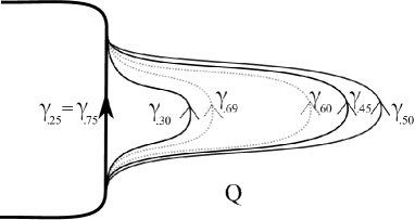
We interpret the chord diagram in Figure 7 as defining an immersion with four regular double-point pairs that we will resolve to create families of embeddings. Two of the double points are decorated in blue, and the other two are decorated in red. The chord decorations , indicate that the ‘shortcut’ loop , when projected to the factor has degree or respectively. The immersion is represented in Figure 8 (left).
Resolving this immersion would give us a map
We pre-compose with the map given by where is a map with . The choice of degree is governed by the signs in our chord diagram. The composite , when restricted to is null, giving us, after a small homotopy of , a commutative diagram
We proceed computing the homotopy-class of in steps. We will see that is null-homotopic, thus . In general, one can prove an analogous theorem to Proposition 3.2, computing precisely. The exponent of this group can be shown to be equal to . The group is one of the stable homotopy groups of spheres, and is known to be finite. When needing to compute the order of precisely, one constructs the closure as in Proposition 3.2, giving the map . The homotopy group can be described in terms of homotopy-groups of spheres via the homotopy-equivalence giving
| \psfrag{p}[tl][tl][0.7][0]{p}\psfrag{q}[tl][tl][0.7][0]{q}\psfrag{+}[tl][tl][0.5][0]{+}\psfrag{-}[tl][tl][0.5][0]{-}\includegraphics[width=170.71652pt]{gpq_res.eps} \psfrag{p}[tl][tl][0.7][0]{p}\psfrag{q}[tl][tl][0.7][0]{q}\psfrag{+}[tl][tl][0.5][0]{+}\psfrag{-}[tl][tl][0.5][0]{-}\includegraphics[width=170.71652pt]{gpq_res2.eps} |
The homotopy-class of a map is determined by the homotopy classes of the projections: (a) and (b) (two maps) . By the Pontriagin construction, the latter two maps are determined by framed cobordism classes of -manifolds in , taking the pre-image of any point that is not the base-point of the sphere. The projection is determined by a framed cobordism class of a countable collection of disjoint -manifolds in . A simple way to construct these manifolds is to take the cohorizontal manifolds, i.e. fix a unit direction . Define consisting of pairs of points such that the displacement vector is a positive multiple of . Then given we lift the map to the universal cover of , interpreted as the submanifold of such that the points have disjoint -orbits. We take the pre-image of . This manifold family (as a function of ) is precisely what we need to detect the Laurent polynomial associated to the homotopy-class of the projection .
| \psfrag{a}[tl][tl][0.7][0]{\alpha}\psfrag{b}[tl][tl][0.7][0]{\beta}\psfrag{tbwkj}[tl][tl][0.7][0]{t_{2}^{\beta}.w_{32}}\psfrag{tawij}[tl][tl][0.7][0]{t_{2}^{\alpha}.w_{12}}\psfrag{ta}[tl][tl][0.7][0]{}\psfrag{tb}[tl][tl][0.7][0]{}\psfrag{pi}[tl][tl][0.7][0]{p_{1}}\psfrag{pj}[tl][tl][0.7][0]{p_{2}}\psfrag{pk}[tl][tl][0.7][0]{p_{3}}\psfrag{0}[tl][tl][0.7][0]{0}\psfrag{R}[tl][tl][0.7][0]{{\mathbb{R}}}\includegraphics[width=170.71652pt]{coleg.eps} |
Rationally the class is a linear combination of Whitehead products, by Proposition 3.1. To determine the linear combination, we use an idea from [BCSS], where it was shown that certain collinear (trisecant) manifolds can detect Whitehead products in . The key property of the collinear manifolds is they (a) they suffice to detect the generators of , and (b) there is more than one path-component to these manifolds, allowing one to go further and detect Whitehead products . This allowed the authors in [BCSS] to express the type-2 Vassiliev invariant of knots as a linking number of trisecant manifolds, and further as a count of quadrisecants. Consider to be the submanifold of where the points sit on a straight line in in that linear order. Similarly, define to be the submanifold of such that sit on a straight line, in that linear order. These two manifolds are disjoint, moreover the former manifold detects the homotopy-class , and the latter detects , thus the preimage of the disjoint pair by the map is a -component Hopf link in . This is a non-trivial framed cobordism class of disjoint manifold pairs, as the linking number of the two components is . Moreover, this linking number is zero if we use the map provided .
The invariant is therefore computable via the linking numbers of the pre-images of the collinear manifolds, i.e. one computes the linking numbers of the pre-images of and via the lift of to the universal cover of . This is the coefficient of in .
Unfortunately the above is a relatively delicate visualisation task. See [BCSS] for examples of how one can directly compute linking numbers of trisecant manifolds. We use a variation of an argument of Misha Polyak [Po]. Polyak gave a direct argument showing that the quadrisecant formula of [BCSS], itself a linking number of trisecant manifolds, can be turned into a Polyak-Viro formula, i.e. a count involving only cohorizontal manifolds. Interestingly, Polyak’s argument is done using maps out of -point configuration spaces, while ours uses submanifolds of -point configuration spaces.
There is cobordism of the manifold pair and . A cobordism between these two families is given by the parabolic spline family. Specifically, fix a direction vector . Let be the orthogonal compliment to in . Let be a line, and be a quadratic function whose second derivative with respect to arc-length on is given by . Thus when the graph of the function can be any line in except those parallel to the direction. Thus as a family parametrized by we have a cobordism between and .
There is an important technical issue here as the family is not disjoint when , as it allows for triple points in the direction. This does not pose a problem for us, since generically we can assume in our family the direction vectors of collinear triples form a closed co-dimension subset of , i.e. the compliment is open and dense, thus generically we can choose to be disjoint from this set. So we can compute the coefficient of in as the linking number of the pre-image of the above pairs, for .
Our strategy then, given is to first construct the framed cobordism class representing in the language of cohorizontal manifolds. This allows us to explicitly construct a null-cobordism corresponding to a null-homotopy of . We then move on to study . The null-cobordisms associated to can now be attached to the boundary of , giving us a framed cobordism representation of , where .
Example 3.6.
By careful choice of the immersion defining we can arrange that there is a unique parameter value in where the embedding lives in and the associated planar diagram has eight regular double-points. Moreover, we can ensure the locus of parameters in such that the associated embedding has double points is the wedge of two embedded copies of in , parallel to the coordinate axis, i.e. considering to be with the boundary collapsed. The resolution with the eight regular double points is depicted in Figure 8. Four of the double points persist along the red coordinate axis (i.e. a copy of ) and the remaining four persist along the blue coordinate axis. Considering the evaluation map , the submanifold of mapping to cohorizontal points is depicted in Figure 10. This manifold is the disjoint union of four embedded spheres, diffeomorphic to . There are two such spheres along the blue coordinate axis, consisting of the sphere where the point is above the , and the sphere where the reverse is true; the point is above the . Similarly there are two such spheres corresponding to the red coordinate axis. These sphere are essentially linearly-embedded in , having disjoint convex hulls, i.e. they are unlinked. Moreover, these spheres bound four disjointly-embedded balls, .
| \psfrag{1}[tl][tl][0.5][0]{1}\psfrag{4}[tl][tl][0.5][0]{4}\psfrag{8}[tl][tl][0.5][0]{8}\psfrag{12}[tl][tl][0.5][0]{12}\psfrag{16}[tl][tl][0.5][0]{16}\psfrag{c2i}[tl][tl][0.7][0]{C_{2}[I]}\psfrag{RBn}[tl][tl][0.7][0]{{\color[rgb]{1,0,0}B^{n-2}}}\psfrag{BBn}[tl][tl][0.7][0]{{\color[rgb]{0,0,1}B^{n-2}}}\psfrag{r12}[tl][tl][0.7][0]{t^{-q}Co_{1}^{2}}\psfrag{r21}[tl][tl][0.7][0]{t^{q}Co_{2}^{1}}\psfrag{b12}[tl][tl][0.7][0]{t^{-p}Co_{1}^{2}}\psfrag{b21}[tl][tl][0.7][0]{t^{p}Co_{2}^{1}}\includegraphics[width=284.52756pt]{gpq_t2.eps} |
Our ‘units’ for in Figure 10 are the indices for the cohorizontal points, along the parametrization of the embedded interval, suitably rescaled. The four spheres in the preimage are trivially framed, thus the disjoint balls they bound gives a null-cobordism. Thus Figure 10 depicts the framed cobordism classes of and for all . The bounding discs can be thought to be depicted in the black arcs connecting the red and blue cohorizontal points, but these also trace out the cohorizontal points through the end homotopies. The bounding discs for the manifolds determine null-homotopies of the maps , while we assert that the corresponding bounding discs for the manifolds determined by the null-homotopy are as depicted.
In Figure 11 we depict projections of the manifolds . The domain of is a copy of but we think of this sphere as a ball with its boundary collapsed to a point. The ‘ball’ being with four triangular cylinders attached, due to the null-homotopies. The projection in Figure 11 is to the (union triangular cylinders) factor. We use as our coordinates for . In the figure and are the planar coordinates, with pointing out of the page. One therefore obtains Figure 11 from Figure 10 by considering how the cohorizontal points from Figure 10 induce cohorizontal points on the boundary of Figure 11. One then fills in the interior arcs: for example if there is a point on the boundary facet of , then there will be an entire straight line parallel to the -axis. Thus the interior arcs will be orthogonal to the page in this projection. One then appends the null-cobordisms to the boundary facets of .
For example, the manifold labelled consists of three parts in the figure. There are two arcs parallel to the coordinate -axis, these are represented by the short arcs between the nearby pairs of blue points. In this represents two disjoint -balls. There are also two longer diagonal arcs labelled , one overcrossing and one undercrossing. The overcrossing indicates the null-cobordism coming from the attachment on the face of , while the undercrossing represents the null-cobordism attached on the face.
Pairwise these linking numbers are all zero, with the sole exception of the pair , which gives . We have suppressed the diagrams for the linking numbers of the preimages of the pairs , , and , as their computations are analogous.
| \psfrag{c2i}[tl][tl][0.7][0]{C_{3}[I]}\psfrag{RBn}[tl][tl][0.7][0]{{\color[rgb]{1,0,0}B^{n-2}}}\psfrag{BBn}[tl][tl][0.7][0]{{\color[rgb]{0,0,1}B^{n-2}}}\psfrag{q12}[tl][tl][0.7][0]{t^{-q}Co_{2}^{3}}\psfrag{mp21}[tl][tl][0.7][0]{t^{p}Co_{3}^{1}}\psfrag{p12}[tl][tl][0.7][0]{t^{-p}Co_{2}^{3}}\psfrag{mq21}[tl][tl][0.7][0]{t^{q}Co_{3}^{1}}\psfrag{t1}[tl][tl][0.7][0]{t_{1}}\psfrag{t3}[tl][tl][0.7][0]{t_{3}}\psfrag{c23c31}[tl][tl][1][0]{lk({\color[rgb]{0,0,1}Co_{3}^{1}},{\color[rgb]{1,0,0}Co_{2}^{3}})}\psfrag{c31c23}[tl][tl][1][0]{lk({\color[rgb]{1,0,0}Co_{3}^{1}},{\color[rgb]{0,0,1}Co_{2}^{3}})}\includegraphics[width=341.43306pt]{gpq_lk.eps} |
Proposition 3.7.
The homotopy group is abelian, for all .
Proof.
A diffeomorphism of can be isotoped canonically so that its support is contained in where , i.e. we can effectively rescale the diffeomorphism radially in the factor. Using conjugation by a translation in the factor, one can show that up to isotopy, diffeomorphisms of can be assumed to have support in where is any open subset of . ∎
Let denote the subgroup of of elements homotopic to the identity. This is a subgroup of index in and index two in the subgroup acting trivially on .
Theorem 3.8.
Any two elements of , the group of diffeomorphisms homotopic to the identity, commute up to isotopy.
Proof.
Any element of is isotopic to one that fixes a neighborhood of pointwise. Thus commutativity follows as in the proof of the first part of Proposition 3.7.∎
Let denote the space of smooth embeddings that restricts to the standard inclusion on the round boundary . Denote the corresponding framed embedding space by . This space consists of pairs where and is a trivialization of the normal bundle to that restricts to the canonical trivialization on . Both and are contractible spaces, the proofs are analogous to the homotopy classification of collar neighbourhoods. The role these embedding spaces play is as the total spaces of fiber bundles. The half-ball is defined in Definition 2.4.
The first fiber bundle to consider is where denotes the unknot component of , i.e. the path-component of the linear embedding. This bundle is in principle useful, but the fiber is embeddings of into which are fixed on their boundary, which is not a very familiar space. By taking the derivative along the boundary we see this space fibers over with fiber homotopy-equivalent to . This latter space is the space of embeddings which restricts to the inclusion on , where is some preferred point. These fiber bundles were used in an analogous way by Cerf [Ce2] in his appendix, Propositions 5 and 6.
Alternatively we can form the bundle
where the base space consists of embeddings together with a normal vector field along the embedding i.e. The fiber of this bundle is technically the embeddings of into which agree with the standard inclusion (and its derivative) along . This fiber has the same homotopy type as .
Similarly, we have the corresponding bundles for the framed embedding spaces
Given that the total space is contractible, this allows us to describe the unknot component of these embedding spaces as classifying spaces.
Lemma 3.9.
We take a moment to unpack some of the underlying geometric ideas involved in the lemma.
There is an isomorphism of homotopy groups
moreover, this map has an explicit geometric description. To do this, we need the exact fiber of the bundle . This is the space of embeddings of into which agrees with the standard inclusion and its derivative on the full boundary of . Denote this space by . Serre’s homotopy-fiber construction tells us that is homotopy-equivalent to
In the above, denotes the basepoint of , i.e. the standard inclusion . The homotopy-equivalence between is given by associating to . The homotopy-equivalence between and is given by associating to where .
For the sake of those not familiar with these methods we describe the homotopy-equivalence directly. For this we need to adjust our model slightly. We replace the space with the homotopy-equivalent space of embeddings where the support is constrained to be in , i.e. the maps are the standard inclusion outside of . Similarly, would be the space of embeddings with a normal unit vector field, the embeddings and normal vector required to be standard outside of . From this perspective, the fiber is the space of embeddings where the support is not only contained in , but the embedding and its derivative in the normal direction is required to be standard on . Observe the explicit deformation-retraction of to a point, given by associating to the path (as a function of ), where
Thus the map in this model is the one that associates to the path given by
The vector field being . So it would be reasonable to call this map slicing the embedding.
We mention a few elementary consequences of Lemma 3.9.
For embeddings with -dimensional domains we have
The space is a bundle over , and this space is equal to when . The fiber of this bundle is , provided . This bundle is known to be trivial. One trivialization can be expressed as a splitting at the fiber . To construct it, use the null-homotopy of the Smale-Hirsch map [Bu1] . Given that the normal vector field is orthogonal to the Smale-Hirsch map, one can use the holonomy on to homotope the normal vector field canonically to a map orthogonal to the -axis, giving the map , and the splitting
Theorem 3.10.
Raising the codimension by one, and provided we get the identification
When , is a monoid under concatenation, isomorphic as a monoid to , therefore with inverses. When , is a commutative monoid under concatenation, therefore an abelian group, isomorphic to .
The space has a concatenation operation, which could also be thought of as an action of the operad of -discs. The space similarly has a concatenation operation with one less degree of freedom. It can be encoded as an action of the operad of -discs. These discs actions turn the two sets and into commutative monoids with the concatenation operation, provided . Moreover, one can see that the concatenation operation and concatenation of loops are the same operation on . Thus, the isomorphism is an isomorphism of groups, which must be abelian. Lastly, notice that fibers over with fiber , provided . So for all we have a homotopy-equivalence
Corollary 3.11.
Since the concatenation operation on turns into a group, it makes sense to consider the fiber bundle
Every embedding that is standard on is the fiber of some trivial smooth fiber bundle with fiber , by Lemma 3.9 and isotopy extension. Thus acts transitively on . We record the observation.
Theorem 3.12.
The group acts transitively on . Moreover every reducing ball is the fiber of some smooth fiber bundle .
Alternatively attach a to obtain where the reducing ball is now an -ball with boundary a standard -sphere. By the Cerf - Palais theorem there is a diffeomorphism of this sphere taking to a standard n-ball fixing pointwise.
Theorem 3.13.
The group acts transitively on the non-separating -spheres in . Moreover, every non-separating -sphere is the fiber of a fiber bundle .
Proof.
Provided this is classical. When observe that complementary to a non-separating sphere there is an embedding that intersects the sphere precisely once and transversely. Since , we can isotope our embedding to be equal to and similarly isotope our non-separating sphere. If we drill a neighbourhood of out of we have constructed , and our non-separating sphere is converted to a reducing ball. The result follows from Theorem 3.12. ∎
Let denote a fixed . Let (resp. denote the component of that contains the standard inclusion to (resp. , where is a closed regular neighborhood of . Note that the restriction map is a fiber-bundle with fiber having the homotopy-type of one path-component of the free loop space of . The map given by deleting the interior of is a homotopy-equivalence.
Lemma 3.14.
The locally trivial fiber bundle induces a long exact homotopy sequence whose final terms are
Here is induced by isotopy extension and is induced by extension which is the identity on the complementary .∎
Most of the rest of the paper will be spent showing that there is a homomorphism which when composed with gives rise to a homomorphism, of the same name, such that is trivial. Furthermore, there exists an infinite set of elements of whose images are linearly independent. From this we will obtain the following result whose proof will be completed in §8. A sharper form of this result is given as Theorem 8.5.
Theorem 3.15.
Both the group and
contain an infinite set of linearly independent elements.
4. 2-Parameter Calculus
This section introduces techniques for working with 1 and 2-parameter families of embeddings of the interval into a 4-manifold.
4.1. Spinning
We start by setting conventions for the operation we call spinning that other authors call double point resolution. Spinning about arcs is an operation that generates , the Dax subgroup, i.e. the subgroup represented by loops that are homotopically trivial in [Ga2]. Here is an oriented properly embedded in the oriented -manifold with a fixed parametrization.
Definition 4.1.
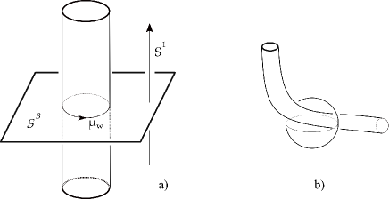
Let be an oriented 2-sphere in with . Given an embedding with and , we obtain a based loop in by using to drag around . Let be a small arc containing . is defined so that for , is a small arc containing , where is an embedded arc in . During , keeping endpoints fixed, rotates around . I.e. view with and identified to points and for for monotonically increasing . Finally during , returns to following the reverse of . Corners are rounded so that each is smooth. The local picture of spinning about is shown in Figure 12. The direction of the spinning is determined by the rule that (motion of , orientation of ) gives the orientation of . Any loop in , isotopic to one constructed as above is called a -spinning of about . The spinning that goes about in the opposite direction is called a -spinning of about .
 |
Lemma 4.2.
Spinning depends only on the orientation of , the orientation of and the relative path homotopy class of , i.e. if is a path homotopy of to , then we require that . ∎
If is an embedded arc from to the oriented arc , then let be a 3-ball normal to at oriented so that (orientation of , orientation of )=orientation of . is called a normal 3-ball. Let oriented with the outward first boundary orientation and . Define the spinning about to be the ’-spinning about . Chord diagram notation for this spinning and its inverse are shown in Figure 13a). The sign denotes whether this is a positive or negative spinning. Band/lasso notation is shown in Figure 13b). The band with being the core of the band and a lasso is a circle in containing, up to a small isotopy and rounding corners, . and are shown in Figure 13d) and in Figure 13c). The positive (resp. negative) spinning corresponding to the band and lasso will be denoted (resp. ). We call the base of the band and the top of the band. We orient the core of the band to point from the base to the top.
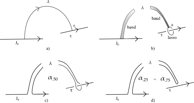 |
For this section and the next we view as with the product orientation. Let be a properly embedded arc in . When , or very close to it, the of Figure 13) will be replaced by , where is viewed as the basepoint. Unless said otherwise all charts of will be of the form , where the -direction is the -direction. Spinnings will almost always be about oriented arcs in a with the band . Here the normal ball intersects in a 2-disc called the lasso disc with the lasso its boundary. We call the lasso 3-ball and the lasso sphere. In this paper, given a lasso, the lasso disc, sphere and 3-ball will be clear from context. The spinning will be denoted L/H (resp. H/L) if the homotopy from to first goes into the past (resp. future) and then into the future (resp. past).
We now give an oriented intersection theoretic way to decide whether or not a spinning of about an oriented arc is positive or negative. First, orient the band to be coherent with its intersection with as in Figure 14 and then orient the lasso disc to be coherent with as in Figure 14.
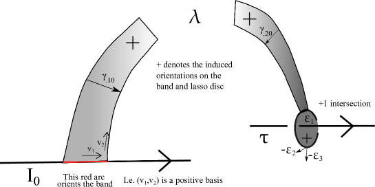 |
Lemma 4.3.
The spinning is positive if and only if the spinning is L/H (resp. H/L) and the oriented intersection number of with the lasso disc is +1 (resp. -1).
Proof.
Let denote the standard orientation of . We can assume that defines the orientation of so that the orientation of a normal ball is given by . We can also assume that the band and lasso appear as in Figure 14), i.e. so that is an outward normal to and an orienting vector for is . Therefore, is oriented by and if the spinning is , then the motion vector for is when the tangent vector to is . It follows that the lasso disc has intersection +1 with . The H/L case follows similarly.∎
Lemma 4.4.
The spinnings of Figure 15 a) - d) and e) - f) are homotopic in . Furthermore, the homotopy from a) to b) is supported in the union of a small 4-ball that contains the bands and the 3-balls spanning the spinning spheres and . The homotopies from b) to d) are supported in a small neighborhood of the union of the bands and the sphere . The homotopy from e) to f) is supported in a neighborhood of the arc. Note that going from e) to f) the changes sign, the arc changes orientation and the +/- changes to -/+.
 |
Proof.
The assertions regarding a) to b) are immediate. To go from b) to c) first choose coordinates so that a neighborhood of the top of the band as well as the lasso are contained in the plane and near the top of the band, the core of the band lies in the -axis. Next rotate to take the lasso to its reflection in the -axis. This is achieved by a rotation of the plane. Finally, a rotation in the plane isotopes the band back into . Using a different rotation we could have obtained the opposite crossing. Apply this homotopy twice to go from c) to d). Using Lemma 4.3 the assertions regarding e) and f) follows from that of a) and b). ∎
Remark 4.5.
This lemma implies that the core of a band determines the isotopy class of the band up to possibly adding a half twist. Thus the isotopy class of the band is determined by the core arc and the orientation on the lasso disc.
Lemma 4.6.
Let be parallel oriented embedded arcs from to whose positive endpoints intersect in a subarc as in Figure 16 a). Let (resp. denote the spinning corresponding to (resp. with that of being oppositely signed. Then, the loop in which is the simultaneous spinning of and is homotopically trivial via a homotopy whose support lies in a small neighborhood of a parallelizing band between and .
More generally, let be the two spinnings as in Figure 16 b). Here the spinnings are expressed in band/lasso notation. Except for neighborhoods of the base arcs, where they differ by a half twist, the bands and are parallel, connecting to parallel lassos and parallel lasso spheres and . Then, is homotopic to via a homotopy supported in the union of a 4-ball about the non parallel parts of the bands as in Figure 16 c) and a small neighborhood of the parallelism between the spheres and the bands. ∎
 |
Definition 4.7.
The pair of spinnings defining above is called a parallel cancel pair. Here and are carried by a branched band surface. The arcs in and where the bands diverge are called the branch loci. A homotopy as in Lemma 4.6 is called the undo homotopy.
Definition 4.8.
Let be a -spinning about the 2-sphere . Suppose that a 3-ball and a properly embedded 2-disc with transverse to as in Definition 4.1. Let be the result of compressing along . Then is homotopic to a concatenation of two spinnings along nearby ’s, where spins about . The operation of replacing by is called splitting. The reverse operation is called zipping. See Figures 16d) and e).
Remarks 4.9.
i) The support of the homotopy from to can be taken to be a small neighborhood of .
ii) Suppose that is presented by the band and lasso . Suppose that denote the lasso sphere, disc and 3-ball. Let and be obtained from by removing a small neighborhood of its core and let and be the components of and , where and are obtained from by removing a small neighborhood of a properly embedded arc which intersects at its core. Then is a splitting of and we call a splitting of . They are spinnings about and , the components of , where is a properly embedded 2-disc such that . Here we require that the spinning across and be L/H (resp. H/L) if the spinning across is L/H (resp. H/L). Note that is homotopic to by a homotopy supported in a small neighborhood of .
iii) As an application, suppose that are the local edges of a 1-complex emanating from the vertex . If is a -spinning about a subarc of close to , then splits to a concatenation via a homotopy supported away from . Figure 17 a) and b) demonstrates the argument for .
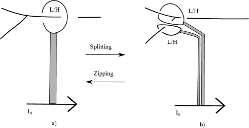 |
Definition 4.10.
An abstract chord diagram in the manifold consists of
a) an oriented properly embedded arc
b) finitely many pairwise disjoint ordered pairs of distinct points in with linearly ordered by the orientation on
c) For each
d) For each .
Remarks 4.11.
1) An abstract chord diagram in a 4-manifold gives rise to an , well defined up to homotopy, which is a concatenation of spinnings, by choosing pairwise disjoint embedded paths from to representing . Call such paths chords. An abstract chord diagram together with chords is called a realization and sometimes just called a chord diagram. Since spinnings commute as elements of ), this element is unaffected by modifying the relative location of the pairs of points , however most of the abstract chord diagrams of interest in this paper represent the trivial element, up to homotopy and we are not free to move these points in general. We will be considering the following types of modifications.
Definition 4.12.
We have the following operations on abstract chord diagrams.
i) (reversal) is replaced by )
ii) (exchange) If are adjacent in the linear ordering where and , then replace by and by .
iii) (sliding) As input, is adjacent to an with . As output the chord is replaced by three chords , , . Here is moved to the other side of , Also are order adjacent as are . Sign Rule: if (resp. ) the interval between and (resp. and ) contains none or both of , otherwise and (resp. ) . See Figure 18.
iv) (isotopy) Points are moved isotopically in without any collisions.
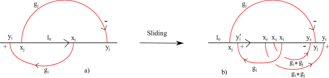 |
Remark 4.13.
Let denote a chord from to . A sliding is the result of splitting the spinning near , then isotoping the resulting lasso that links along and finally do a second splitting near . Note that the support of this isotopy is disjoint from .
Definition 4.14.
We say the abstract chord diagrams on and on are combinatorially equivalent if their data agrees up to reversals and isotopy.
Lemma 4.15.
If the abstract chord diagrams and defined on are combinatorially equivalent, then is homotopic to .∎
Lemma 4.16.
(Change of Basepoint) Let and be path homotopic embedded arcs in the 4-manifold . An abstract chord diagram on induces a combinatorially equivalent chord diagram on . If then is well defined up to homotopy and in particular is independent of the path isotopy from to .
Proof.
Since and are path homotopic, there is a canonical isomorphism between to and hence induces a chord diagram on well defined up to combinatorial equivalence and hence is well defined up to homotopy. Alternatively, we can assume that and agree in a small neighborhood of their initial point and . It follows that the homotopy class of is independent of the conjugating .∎
4.2. Factorization
In this subsection we introduce techniques for constructing and working with 2-parameter families of embeddings. We will define the bracket of two null homotopic loops in whose domain and range supports are disjoint and will show that such brackets are well defined in , anticommute and are bilinear. Our fundamental example is the family in depicted in Figure 19 a) which is the bracket of the 1-parameter families and defined by the blue and red cords. The or means that the indicated cord goes or times about the .
Definition 4.17.
Let be an oriented 4-manifold and a proper embedding with image . Let be an embedding. We define the domain support of and the range support of . If , then define the domain support of and the range support of . Define the parameter support of to be .
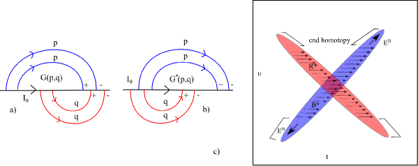 |
Example 4.18.
The domain support of (resp. ) are four small intervals that contain the endpoints of the blue (resp. red) cords while the range support of (resp. is contained in a small neighborhood of the blue (resp. red) cords. Note that both and are null homotopic and have disjoint domain and range supports. is an example of a separable pair which we now define.
Definition 4.19.
Let , the based loop space. We say that the ordered pair is separable if
i) and have disjoint domain supports
ii) and have disjoint range supports
iii) and are null homotopic
Definition 4.20.
If are such that for all have both disjoint domain and range supports, then define by (resp. if ) (resp. and if . is called the adjunction of and .
Definition 4.21.
Let be a separable pair with parameter supports within . Define the bracket of to be , the adjunction of the elements defined as follows.
i) For when and otherwise. when and otherwise.
ii) For , is a null homotopy of such that if . , is a null homotopy of such that if .
iii) for when and otherwise. when and otherwise.
We let denote the class in represented by . The homotopies and are called end homotopies. and are called the midlevel loops of the adjunction .
Example 4.22.
The blue (resp. red) region of Figure 19 c) contains the parameter support of the 2-parameter family (resp. ) arising from (resp. ). The arrows are meant to suggest that as we horizontally traverse the blue or red region, for , we see a conjugate of or .
Remark 4.23.
If the range supports of and are disjoint, then is homotopically trivial.
Lemma 4.24.
(Independence of End Homotopies) If are separable such that for all , then .
Proof.
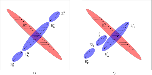 |
Proposition 4.25.
The class is determined by .
Proof.
Let and have the common . Since the domain and range supports of and are disjoint, we can independently reparametrize and so that and coincide for . The Independence lemma implies that they represent the same element of .∎
Definition 4.26.
We denote by the class in induced from . We say that the elements are separable if their domain and range supports, as in Definition 4.17 are disjoint. We call a separable pair. We say that and are separably homotopic if there exist homotopies , such that for each and are separable.
Lemma 4.27.
If and are homotopically trivial and and are separably homotopic, then .∎
Proposition 4.28.
(bilinearity) If is a separable pair, separably homotopic to () where each and is homotopically trivial and denotes concatenation, then .
Proof.
It suffices to consider the case that n and . The result will then follow from induction. First notice that the support of a concatenation is the union of the supports of the terms so that each of and is a separable pair. By the independence of end homotopies we can assume that the end homotopy for is a concatenation of those of and . Since is a concatenation, we can assume that the usual support of , while support . Thus we can assume that appears as in Figure 21 a) and we can split B into two copies of itself as in Figure 66 b) and so . ∎
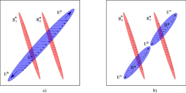 |
Lemma 4.29.
We have the following equalities in where denotes the reversal of .
Proof.
Start with as in Figure 22 a) and then rotate clockwise to obtain Figure 22 b) which represents the same element of . Finally, homotopically reparametrize the rotated and to obtain Figure 22 c) which depicts . Since and have disjoint supports in both domain and range, this reparameterization can be done independently on and subject to the condition that during the homotopy all points that are both blue and red lay in the original region. For this reason the arrows can be made horizontal in only one direction. This argument applied to a counterclockwise rotation shows that . Next note that the standard homotopy from to is through loops that have domain and range supports disjoint from that of and hence thereby establishing the third inequality. The final equality follows from the earlier ones.∎
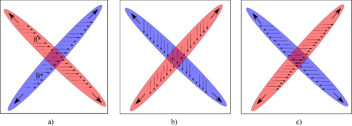 |
Example 4.30.
If are defined by abstract chord diagrams such that , then is separable. That is because the domain support of is contained in and the range support is contained in a small neighborhood of the chords and we can assume that the chords of and are disjoint. Our fundamental example is the separable pair denoted defined by the chord diagram shown in Figure 19 a), where (resp. ) is defined by the blue (resp. red) chords. It’s class in is called the -primitive class. A second basic example is the separable pair denoted shown in Figure 19 b) and called the symmetric .
Definition 4.31.
We say that the abstract chord diagrams and are disjoint if . The sum of disjoint chord diagrams is the union of the data of the diagrams.
Lemma 4.32.
Let and be represented by pairwise disjoint abstract chord diagrams and for .
i) (reversal) If is obtained from by a reversal, then is separably homotopic to . If and are homotopically trivial, then .
ii) (exchange) If is obtained from by an exchange along an interval whose interior is disjoint from , and both B are homotopically trivial, then .
iii) (sliding) If (resp. ) is obtained from (resp. ) by sliding a chord over either a blue or red chord, then (resp. .
iv) (addition/cancellation) If , , are disjoint chord diagrams with the sum of and and , then . The similar statement holds with and switched.
v) (isotopy) If (resp. ) is an isotopy of to (resp. to and for every , , then .
Proof.
i) and v) are immediate. iv) follows from Proposition 4.28. Being the composite of an isotopy and two splittings, it follows from Remark 4.9 that the support of a sliding is disjoint from the chord being slid over. Therefore the homotopy from to is separable. This proves iii). To prove ii) consider the representative Figure 23 a) which shows a chord diagram with the exchange interval indicated. The chord diagram of Figure 23 b) has the same , but the blue chord diagram is given by a parallel pair of oppositely signed arcs representing the same group element. Furthermore, the intervals between their initial points and between their final points contains no points of . Apply the undo homotopy, Lemma 4.6 to to reduce to the trivial diagram. Since the domain and range support of this undo homotopy is disjoint from that of , it follows that . Using bilinearity we obtain Figure 23 c). We again use the undo homotopy to cancel a pair of parallel oppositely signed blue chords to obtain the diagram of Figure 23 d) which has a pair of chord diagrams isotopic to the exchanged pair. ∎
Remark 4.33.
A special case of iv) is when contains a pair of parallel oppositely signed chords with the same group elements, is disjoint from the parallelism between their endpoints and is the chord diagram with the parallel pair deleted, in which case .
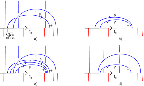 |
Definition 4.34.
Let and be disjoint chord diagrams on . We say that is combinatorially equivalent to if one can be transformed to the other through disjoint chord diagrams that change by reversals, isotopies and allowable exchange moves.
We have the following analogues of Lemmas 4.15, 4.16 which, in combination with Lemma 4.16 have similar proofs.
Lemma 4.35.
If and are combinatorially equivalent, then .∎
Lemma 4.36.
(Change of Basepoint) Let and be path homotopic embedded arcs in the 4-manifold . A pair of disjoint chord diagrams on induces a pair on unique up to combinatorial equivalence. Furthermore, is obtained from by a change of basepoint isomorphism which is independent of the path isotopy from to . ∎
Lemma 4.37.
.
Proof.
The argument is given in Figure 24. Figure 24 a) shows . One of the red chords is reversed to obtain Figure 24 b). That chord is slid over the adjacent blue chord to obtain Figure 24 c). A red chord is then reversed and the resulting pair of oppositely signed red chords with group element are cancelled using the undo homotopy. ∎
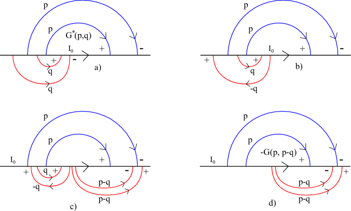 |
4.3. Fundamental Classes
We have already introduced the primitive family . We now introduce the elementary classes and double classes and compute in terms of ’s and in terms of ’s.
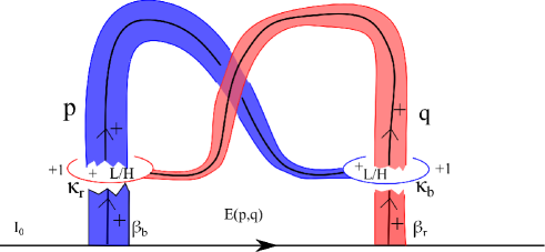 |
Definition 4.38.
Define the standard elementary family by the band/lasso diagram as in Figure 25. In words where (resp. ) is defined by the band (resp. ) and lasso (resp. ), where the base of appears on before the base of . Also (resp. ) links the core of (resp. very close to its base and both spinnings are positive. When the top of the core of (resp. ) is pushed slightly to lie on , then the core represents (resp. ) .
More generally, an family is one of the form where each of and are represented by a single band and lasso where the lasso of one links the core of the other very close to its base.
Remarks 4.39.
i) Up to the ordering of their bases on , twisting of the bands and designation an family is isotopic to the standard for appropriate and , hence up to sign and permutation of and such a family represents .
ii) Recall that the sign of a spinning is determined by a rotation about an oriented sphere, which links an oriented arc . Here, the oriented arcs are the oriented cores of the bands and .
iii) To over emphasize, the order of the base of the bands on and the homotopy classes of their cores determine and . Given such bands, the sign of is determined by the color of the first band, and the signs of the spinnings. The sign of a given spinning is determined by the data and the band core, lasso algebraic intersection number from Lemma 4.3. Thus the sign is given by the parity of the five possible differences from the standard model. In the standard model, shown in Figure 25, we have with +1 intersection number in both cases. That figure also shows the oriented cores of the bands as well as the orientations of the bands and the lasso discs.
Lemma 4.40.
.
Proof.
We first isotope as in Figure 26 a), then homotope it to a chord diagram as in Figure 26 b), where we use Lemma 4.3 to determine the signs of the chords. Use Lemma 4.32 i) to reverse the red chords and then 4.32 iii) to isotope the chords to obtain Figure 26 c). Figure 26 d) is the result of applying two exchanges, Lemma 4.32 ii). A representative of is shown in Figure 26 e). Note that it differs from the standard by a color change and replacing by , i.e. two sign changes at the level. We use bilinearity to add 26 d) and e) and then use the undo homotopy Lemma 4.6 to cancel a pair of parallel red chords to obtain 26 f). Adding Figure 26 g) which is a and then doing an undo homotopy to the red chords we obtain Figure 26 h) which is homotopically trivial, since another undo homotopy eliminates the blue chords. It follows that .
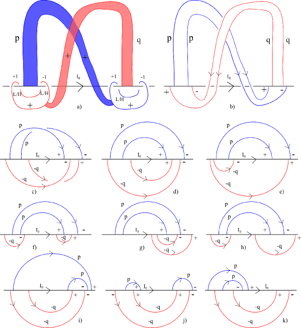 |
Corollary 4.41.
i) if
ii)
iii) (Hexagon Relation) .
Proof.
Definition 4.42.
Define the standard double family in band/lasso notation as in Figure 27. In words, it is of the form where consists of the band and lasso . consists of a parallel cancel pair defined by the bands and lassos . Base, base, base appear in order along . link band just above its base and links band, band at the branch loci. When the top of the bands are pushed to lie on then represents and both represent . Also, the spinning of about the oriented cores of is positive. The spinning of ) (resp. about the oriented core of is positive (resp. negative).
More generally, we call a family a family if up to isotopy it is represented by bands and lassos as a standard family, up to switching the roles of and designations and twisting of the bands.
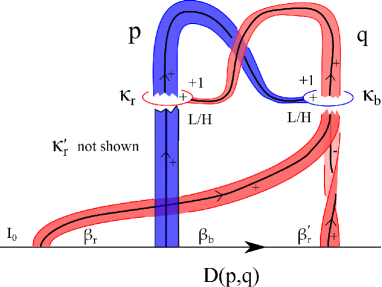 |
Remarks 4.43.
i) Up to sign and permutation of and a family represents the class .
ii) The order of the base of the bands and the homotopy classes of their cores determine and . Given such bands, the sign of is determined by the color of the first band on , and the signs of the spinnings. Here, we need not consider the spinning from since it is always opposite that of . If we use data and intersection numbers to determine the spinnings, then as before the final sign is given by the parity of the five possible differences from the standard model.
Lemma 4.44.
.
Proof.
First note that is a separable family. By construction is a concatenation of and and each is homotopically trivial. Applying bilinearity to Figure 27 we obtain and of Figures 28 a), b). is homotopic to the standard after a blue/red switch, thus . Similarly, the family in Figure 28 b) gives . Here there is a single sign change from the standard arising from .∎
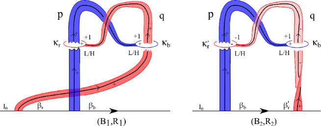 |
Corollary 4.45.
Corollary 4.46.
i)
ii)
iii)
5. Barbell Diffeomorphisms
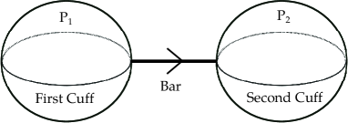 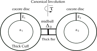
|
(a) (b)
In §2 we defined the families and each of which generated , where is the standard vertical . In §3 we noted that isotopy extension applied to an or gives rise to an element of which is conjecturally isotopically nontrivial. In this section we explicitly identify these diffeomorphisms, the foundational observation being that each is supported in a single . We call such a space a thickened barbell , the barbell itself, a spine, being the disjoint union of two oriented 2-spheres together with an oriented arc that joins them. See Figure 29(a). We will see that and is generated by the barbell map. The barbell map is the result of applying isotopy extension to a loop of a pair of properly embedded arcs in , where a subarc of the first arc is standardly spun around the second and then restricting to the closed complement of these arcs.
By embedding the barbell in another space and pushing forward the barbell map we obtain elements of an operation we call barbell implantation. Implantations yielding elements of induced from the ’s and ’s will be described. Other implantations that we will prove to be isotopically nontrivial in both and modulo will be given in the next section. For we offer explicit candidates including the ones arising from the ’s via filling with an . We will show how to construct the image of and under implantation, thereby exhibiting possibly knotted nonseparating 3-balls (resp. 3-spheres) in (resp. in ), inducing knotted 3-balls in . Some of these will be shown to be non trivial in later sections. For we will show that some barbell maps are order at most 2. Finally, we note that barbell maps extend and generalize the graph surgery diffeomorphisms of Watanabe [Wa1].
We start by defining the model barbell and its thickening in , along the way establishing conventions and identifying various subspaces.
Definition 5.1.
The model barbell is the union two 2-spheres in of radius respectively centered and together with the arc called the bar that points from the first sphere to the second called . These spheres are called the cuffs with (resp. ) being the first (resp. second) cuff. Construct the underlying space of a model thickened barbell by first taking an -neighborhood and then taking the product with . Here and is small. The space is called a thick cuff and the closed complement of the thick cuffs is called the thick bar. The properly embedded 2-disc normal to and centered at is called the cocore disc to . centered at is defined and named analogously. Let denote the canonical involution of induced from the involution on corresponding to rotating the plane by at the point and fixing the coordinates. Define to be the properly embedded transverse 3-ball to the dual arc at and call it the midball. See Figure 29(b). Let . Let where is the closed complementary 3-ball region of . View as the cocore of the 3-handle .
We give the orientation induced from . We orient so that at is a positive basis and orient so that at , is a positive basis. Here is the standard positive basis for . Note that . Use to push forward the orientations on to ones on . Use to positively orient the bar and to orient .
A barbell in a 4-manifold is a subspace diffeomorphic to the model barbell with oriented cuffs and bar such that the cuffs have trivial normal bundles. A thick barbell in a 4-manifold is an embedded together with a barbell spine.
The following is standard.
Lemma 5.2.
-
•
with generators .
-
•
with generators .
-
•
with generators .∎
Construction 5.3.
We now define the barbell map . Let and hence is the closed complement of where . A loop in based at that is fixed near and avoids induces a diffeomorphism of by isotopy extension whose proper isotopy class depends only on the based homotopy class of that loop. To define the path we construct two discs , where is a parallel copy of having been pushed off in the direction and is a disc that coincides with near its boundary and defined below. is a loop that first sweeps across and then sweeps back using . In what follows for , let denote .
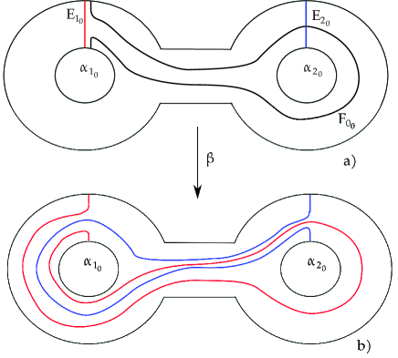 |
We describe as follows. It will intersect each in an arc whose ends coincide with that of . Here lies in the plane and is shown in Figure 30 a). As increases (resp. decreases) slips to the -side (resp. -side) of . For close to , coincides with .
The images of are shown in Figure 30 b). As t increases (resp. ) slips to the -side (resp. -side) of (resp. ). Note that coincides with near its boundary.
Remarks 5.4.
i) An orientation preserving diffeomorphism of supported in the thick bar that is a full right hand twist of the -plane as one traverses the bar does not change the isotopy class of the barbell map, since it fixes setwise, hence does not change the based isotopy class of the loop .
ii) The barbell map is the result of applying isotopy extension to a positive -spinning of about where is a straight arc from to and each is oriented by . It follows from Lemma 4.4 that the barbell map is also the result of a negative spinning of about .
Lemma 5.5.
In ,
i)
ii) ∎
The next result follows by construction.
Theorem 5.6.
is isotopic to .
Theorem 5.7.
and is generated by the barbell map.
Proof.
Let . Since fixes pointwise it is orientation preserving. Its effect on is as follows.
a)
b)
c) for some .
Since fixes a) follows. Apriori, . Since fixes , and . Now double to obtain and extend to so that is the identity outside of . In the double becomes a and the doubled becomes the 2-sphere , both in the first factor. Since has trivial normal bundle as does and it follows that . In a similar manner . Therefore if , then and hence .
Definition 5.8.
Let be a properly embedded 3-manifold in the 4-manifold . We say that is obtained from by embedded surgery if there is a sequence such that is obtained from the regular neighborhood by first attaching a single 4-dimensional handle embedded in and then restricting to some relative boundary components.
Construction 5.9.
We construct by embedded surgery. To start with, is isotopic to the 3-ball obtained from by two embedded 2-handle surgeries where the second 2-handle attachment is given by the cocore of the first as in Figure 31 a). More precisely, the first 0-framed 4-dimensional 2-handle is attached to link and intersect in a cocore . Further if is the result of this embedded surgery, then all , where is as in Construction 5.3. The second 2-handle is a normal neighborhood of and hence is disjoint from . Since is obtained by removing a small subdisc and replacing it by a disc , it follows that is obtained by removing a solid torus, the unit normal bundle of , and reimbedding it as the unit normal bundle of . Finally, is obtained by isotoping the attaching zone of to lie in . At the 3-dimensional level is obtained from by 0-surgery along a Hopf link.
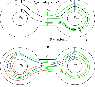 |
Remark 5.10.
Note that if are parallel copies of with closest to ,
then are parallel copies of . The corresponding 2-handles
(resp.
nest, one inside the previous.
Definition 5.11.
Let N be a 4-manifold and a smoothly embedded barbel with framed cuffs. Let be an -regular neighborhood. There is an orientation preserving diffeomorphism that restricts to one from to the model barbell , which essentially preserves normal fibers of the thickenings. Pulling back the barbell map induces a map , well defined up to isotopy. The operation that starts with a framed cuffed barbell and produces up to isotopy, is called implantation. Here can be viewed as an element of or .
Remarks 5.12.
If is oriented we can assume that the framing of the cuffs together with the orientation of the cuffs agrees with the orientation of . Different framings of the bar will give rise to maps and that differ by a twist as in Remarks 5.4 i). That remark also shows that is isotopic to . Thus when is oriented the isotopy class of depends only on the embedding of the barbell and the framing of the cuffs. When the framing is implicit, then depends only on the embedding.
By chasing orientations we obtain:
Lemma 5.13.
If is a barbell in , then reversing the orientation of without changing the orientations on the barbell changes the implantion to its inverse.
We now give a bundle theoretic interpretation of the barbell map. Consider the fiber bundle from the group of diffeomorphisms of to the space of embeddings of two copies of into itself. To define this bundle, we fix two disjoint -discs embedded in the interior of a fixed . The bundle comes from restricting a diffeomorphism to the sub-discs. Not only it is a fiber-bundle, but it is null-homotopic, Proposition 5.3 [Bu2]. Thus there is an injection , moreover the co-kernel of this injection is isomorphic to .
has the homotopy-type of . Thus we have
The factor corresponding to is what generates the barbell diffeomorphism. We have a short-exact sequence
We consider to be , i.e. as a trivial -bundle over . Then as a bundle over , denote the group of fiber-preserving diffeomorphisms of that are the identity on the boundary by . By design, this group is the loop-space on , thus we have shown there is a short exact sequence
Proposition 5.14.
valid for all and all .
The barbell diffeomorphism (family) being the image of the generator in , when .
We now consider implantation where the cuffs of are fixed unknotted and unlinked oriented 2-spheres that are permuted under an elliptic involution of . We assume that , a fixed oriented 3-ball, thereby determining the framings of as in the model barbell. The bar is then determined up to isotopy by its relative homotopy class and hence by a word in the rank-2 free group, the fundamental group of . See Figure 32. With generators as in the figure we will assume that w is reduced and if , then the first (resp. last) letter of is (resp. ). For example, if was the first letter, then it can be removed by rotating fixing pointwise. We denote such a barbell by . It is well defined up to isotopy fixing pointwise. We denote by the corresponding diffeomorphism of which is also well defined up to isotopy.
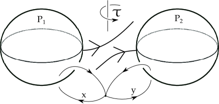 |
Definition 5.15.
We say that is inverse--palendromic if is obtained by first taking its inverse and then everywhere switching and .
Example 5.16.
is inverse--palendromic.
Proposition 5.17.
If is inverse--palendromic, then is isotopic to .
Proof.
Since is inverse--palendromic, is setwise isotopic to via an isotopy that is supported in the bar. The time one map of the isotopy, , is orientation preserving on the cuffs and reversing on the bar. It follows from Theorem 5.6 that is isotopic . ∎
Conjecture 5.18.
. In particular, and are not isotopic to . See Figure 33.
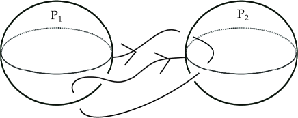 |
Questions 5.19.
i) What are the relations in the subgroup of generated by the ’s?
ii) We can also consider implantations in arising from knotted or linked cuffs. When do these implantations give isotopically trivial diffeomorphisms? What if any are relations amongst these implantations?
Definition 5.20.
Let be a barbell in . Define , the associated sphere to , be the sphere obtained by orientation preserving tubing along the bar to a parallel copy of .
Remark 5.21.
Let be an arc in a normal disc of from to . Then is a barbell whose thickening is isotopic to . The next result shows that if , has thickening with a knotted barbell spine.
Proposition 5.22.
Let be a barbell in . Then
i) is knotted if and only if and hence if , then is not isotopic to .
ii) If , then ’s thickening has no barbell spine isotopic to .
Proof.
i) If , then is obviously unknotted. In general is a ribbon 2-knot whose fundamental group is . Since we can assume that w is a nontrivial reduced word that does not start (resp. end) with a nor end with a it follows that the relator is non trivial and hence the group is non cyclic.
ii) Every non separating embedded 2-sphere in is isotopically trivial. ∎
We now consider implantations where or .
Construction 5.23.
Let a barbell with the implanted map. If is disjoint from the cuffs and transverse to the bar, then is constructed as follows. Let an orientation preserving diffeomorphism, where is the thickened model barbell. We can assume that is parallel 3-balls normal to the model bar. Construction 5.9 shows how to construct the image of these balls under the barbell map. Now pull back by .
Remark 5.24.
is obtained by embedded surgery to where the attaching zone of the 2-handles is the split union of Hopf links. At the 3-dimensional level, is obtained by 0-surgery to the components of this link, thus its topology is unchanged.
Construction 5.25.
(Barbells from Spinning) Let be an embedded oriented in the oriented 4-manifold . Construction 5.3 and Remark 5.4 show that the diffeomorphism of induced by applying isotopy extension to a -spinning of a subarc of about another subarc is the barbell map corresponding to a barbell with linking linking and the bar given by . Applying this to and , denoted in §2 as and , we obtain the barbells shown in Figure 34. To see this for , first consider Figure 34 c) which shows the basic construction and then send to “infinity". We now view these barbells as subsets of and denote them by and . Let denote the corresponding implantations.
| \psfrag{cd2}[tl][tl][0.7][0]{}\psfrag{s1}[tl][tl][0.7][0]{S^{1}}\psfrag{sn}[tl][tl][0.7][0]{S^{3}}\psfrag{f}[tl][tl][0.7][0]{}\psfrag{C}[tl][tl][0.7][0]{c)}\psfrag{D}[tl][tl][0.7][0]{d)}\includegraphics[width=227.62204pt]{FigB7.eps} \psfrag{cd2}[tl][tl][0.7][0]{}\psfrag{s1}[tl][tl][0.7][0]{S^{1}}\psfrag{sn}[tl][tl][0.7][0]{S^{3}}\psfrag{f}[tl][tl][0.7][0]{}\psfrag{C}[tl][tl][0.7][0]{c)}\psfrag{D}[tl][tl][0.7][0]{d)}\includegraphics[width=227.62204pt]{w2_eg4.eps} |
| (a) | The barbell induced from |
|---|---|
| (b) | The barbell induced from |
| (c) | The initial barbell induced from |
| (d) | viewed as a subset of |
Since is obtained by gluing an to elements of extend to elements of . For example, viewing in we obtain the barbell shown in Figure 34 d). Since this barbell is inverse--palendromic its implantation is order at most 2.
Remark 5.26.
Watanabe constructs [Wa1] various -bundles over -spheres to show, among other things, that is non trivial. Specializing his construction to and considering a bundle’s gluing map, give possible nontrivial elements of . He notes that this construction applied to a 4-manifold might yield nontrivial elements of . Here we observe that these diffeomorphisms are compositions of barbell maps. We very briefly outline this in the simplest case when .
Watanabe starts with an embedding of a two vertex arrow graph into and then constructs the corresponding -link in , see [Wa1] §4. We abuse notation by letting denote this embedding when extended to a regular neighborhood. The -link has two components, one Type 1 and one Type 2. Call their respective regular neighborhoods and . Watanabe’s diffeomorphism of , which we denote by , arises from parametrized Borromean surgery of Type 1 on and Type 2 on . Roughly, where and are 2-discs and a 1-disc, the union standardly embedded. where is a 2-disc and are 1-discs and the union is standardly embedded, thus plus a 1-handle. Being a -link, the 1-handle of passes parallel to through . Type 1 surgery effectively replaces by where is the 4-dimensional Borromean rings viewed as a three component tangle in the defining . Thus, Type 1 surgery reimbeds the 1-handle of , hence reimbeds . Let be this new embedding. Type 2 surgery on induces by an arc pushing diffeomorphism and is obtained by pushing forward by . The track of this arc pushing is more or less a disc where is the 4-dimensional Borromean rings. Our assertion follows from the fact that is the composition of two barbell maps. To see this expressed from our point of view, consider as where is a with two open 3-balls and removed. Here, we have two properly embedded discs and that coincide near their boundaries and is obtained by first pushing in along and then out along . The is a , where is a properly embedded arc and intersects each in an arc . and are shown in Figure 35. consists of two subarcs that go around the the second 3-ball . As increases (resp. decreases) slips over (resp. under) and slips under (resp. over) , both returning to coincide with a segment in . This can be done so that for all and hence is embedded. With this description it is evident that and hence , is isotopic to the composition of two barbell maps.
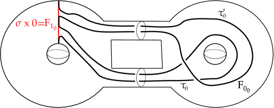 |
6. 1- and 2-parameter families arising from implantations
In the last section we introduced the barbell map and constructed where is the standard separating 3-ball. In this section we slice into 1- and 2-parameter families of discs and arcs. We will show how under barbell implantation into a 4-manifold , where the bar is transverse to a 3-ball, these families produced loops and spheres in and respectively.
Recall that where where and are 3-balls. By scaling to , we henceforth identify with . Let denote the separating 2-disc such that . Recall that for all it follows that . The next result follows by slicing the construction of .
Proposition 6.1.
is isotopic to the family obtained as follows.
i) For , . See Figure 36 a).
ii) For squeeze to create a neck as in Figure 36 b).
iii) For isotope the neck halfway around , going from the side to the side. See Figure 36 c).
iv) For isotope the neck back to its original position shown in Figure 36 b), continuing from the side to the side.
v) For reverse the isotopy from . ∎
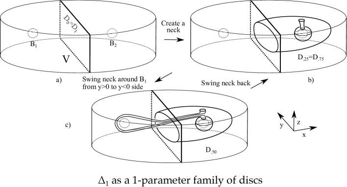 |
Remark 6.2.
is similarly isotopic to the family where we first create a neck connecting discs that surround instead of . For that isotopy the neck swings around going from the side to the side. The neck of is essentially seen in Figure 30 b) where the red arc is replaced by a cylinder. Notice that replacing the blue arc by a cylinder essentially gives the neck of .
We now describe another isotopic family that is neither nor centric. For that isotopy it is convenient to change the base disc to the disc shown in Figure 37 a), via an isotopy of supported in a neighborhood of .
First consider the disc shown in Figure 37 c). This disc is obtained by removing four open discs from , shown in Figure 37 a) and replacing them with two blue discs that surround and two red ones that surround . The red (resp. blue) discs emanate from the first two sheets of the folded that are closest to (resp. ). To go from Figure 37 c) to Figure 37 b)(resp. d)) isotope the blue necks down (resp. up) and the red necks up (resp. down). The region between the blue discs of is a product which can be boundary compressed using a fold of . A similar statement holds regarding the red discs, where the boundary compression starts at the other fold. These boundary compressions are done simultaneously and are supported away from the arc . The result of these boundary compression is shown in Figure 37 e).
Proposition 6.3.
Under the change of basepoint map , the 1-parameter family is isotopic to the following 1-parameter family .
i) For , .
ii) For , is isotoped to the surface shown in Figure 37 b) via the intermediary surface shown in Figure 37 e). This isotopy fixes pointwise. The isotopy for is supported near . For the isotopy restricted to the disc below (resp. above) is supported in the union of a regular neighborhood of and the right (resp. left) hand side of .
iii) For the blue necks are isotoped up and the red necks down to obtain Figure 37 d) with the intermediary shown in Figure 37 c).
iv) For , the isotopy is analogous to the reverse of the to isotopy. Two boundary compressions supported away from produce which is the mirror in the coordinate of .
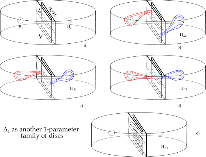 |
Proof.
A direct calculation gives an isotopy between , which by abuse of notation we call and that preserves each slice. Alternatively, let be properly embedded arcs in such that for , and . The loops in induced from and by isotopy extension are homotopic. It follows that and differ by an element of , but that group is trivial by Cerf [Ce2] and Hatcher [Ha1].∎
Since , the factor induces a -fibering on each and hence expresses as a 2-parameter family of intervals. Pushing forward to expresses as a 2-parameter family . Because for all , it follows that we can assume that is supported in .
The family is a bracket as in Definition 4.21. To see this define as the 1-parameter family which only involves the blue discs, so is with two blue discs attached and the passage from to only involves the boundary compression of the blue discs, etc. In an analogous manner we define . The associated 2-parameter families satisfy the conditions of Definition 4.21. The midlevel loops are defined in band lasso notation as in Figure 38 a). For (resp. ) only the blue (red) band and lasso are used. We call the barbell family and all its defining information its data. We have the following result.
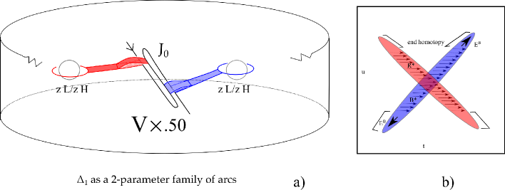 |
Proposition 6.4.
The barbell family is supported in and is homotopic to the separable family of Figure 38 a) described in band lasso notation. The notation means that the spinnings go about the spheres first by going down in the direction and then up. The support of (resp. ) in the parameter space is the blue (resp. red) region shown in Figure 38 b)∎
Remark 6.5.
Note that the end homotopy is homotopic to the undo homotopy.
We now describe how barbell implantation induces an . View as with viewed as . Fixing and , then corresponds to the trivial 2-paraxmeter family by translating within each to . If , then induces a 2-parameter family by naturally translating each so that its end points coincide with that of . Isotopic ’s give rise to homotopic ’s.
Construction 6.6.
Let be an embedding of the barbell neighborhood such that the bar is transverse to and the cuffs are disjoint from . We can assume that , parallel copies of the midball and the -fibering of pulls back to the standard -fibering of each . Further, each is of the form where is a subdisc of and that the projections of to the factor are pairwise disjoint. It follows that is represented by the sum of n 2-parameter families , where is the implantation of . Finally, to construct push forward the data of the barbell family.
Definition 6.7.
For define the 2-parameter families analogously to the family shown in Figure 39 b) where and . Here the red bands go around the just under times while the blue bands go around the just under times. Here the color coding and support in the parameter space are as for the family. Define . is called the symmetric .
Lemma 6.8.
.
Proof.
is obtained by applying Construction 6.6 to the barbell . Each appears qualitatively as up to twisting of the bands near the lasso and whether the individual spinnings are or with differences uniform in . Since any such difference changes the sign of the class in by Lemmas 4.4 and 4.29 the result follows.∎
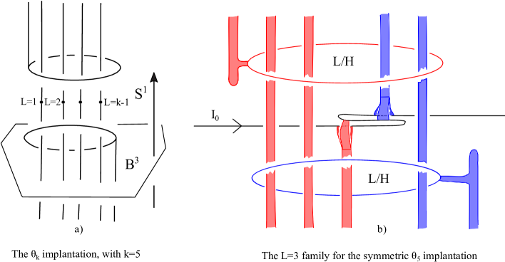 |
Definition 6.9.
Let be an embedding of the barbell such that the cuffs bound disjoint 3-balls and and the bar is transverse to . A reembedding of the bar supported within a small neighborhood of to obtain is called a twisting of . Here the components of the bar that intersect both and the cuffs remain unchanged. is called a twisting of the implantation .
Remark 6.10.
Up to isotopy, a twisting corresponds to replacing arcs that locally link a cuff once to ones that link times.
Definition 6.11.
(Twisting the implantation) Ordering the points through the cuffs and as in Figure 40 a) we construct the implantation. This means that, the ’th (resp. ’th) arc through the (resp. ) cuff now locally links it (resp. ) times. For example see Figure 40 b). The implantation is the implantation twisted by . Define the implantation. See Figure 40 c) for .
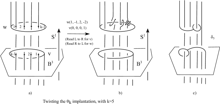 |
Construction 6.12.
Figure 41 shows how to modify a 2-parameter family according to twisting an implantation. Note that modifying a band by a -twist does not change the homotopy class of the 2-parameter family. Therefore, what matters is how many times the modified band goes through the cuff rather than how exactly it is reembedded.
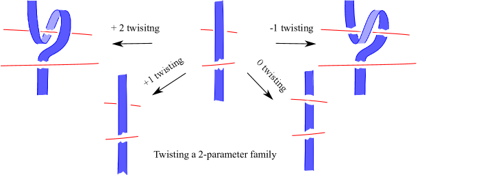 |
Remark 6.13.
In the next section we shall see that gives rise to a matrix with values in such that the sum of the entries equals . Further, at the level, a twisting has the effect of multiplying the ’th row of by and the ’th column by .
7. Factoring the symmetric
In this section we investigate the 2-parameter family ) called the symmetric defined in Definition 6.7. We will show factors into 2-parameter families, giving rise to a matrix with values in equal to those represented by the ’th family. Summing over we obtain which will be shown to be skew symmetric. It will follow that and hence .
As stated in previous sections we view as with the product orientation and denotes a fixed geodesic arc through the origin of .
Definition 7.1.
Fix . For we define properly embedded arcs path homotopic to whose ends also coincide with those of . We first do a small initial isotopy of to obtain the arc of Figure 42 b). To obtain , send the two local top strands just under times positively around the and send the two local bottom strands just under times negatively around the to obtain an embedded arc, as exemplified by or shown in Figure 42 c), d). The 20 strands at the bottom of those figures go around the to attach to the strands at the top.
For homotope each to one based at by shrinking the bands without modifying the lassos. For example, when and , starting with the family shown in Figure 39 b) we obtain the one shown in Figure 43. Denote this 2-parameter as the separable pair , where (resp. ) is defined by the blue (resp. red) bands and lassos.
 |
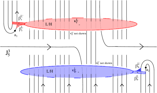 |
Remarks 7.2.
i) By Lemma 4.36, since is path isotopic to and as we shall see can be represented by an abstract chord diagram, it gives a well-defined element of , and so .
ii) Fix . To minimize notation we suppress most of our -subscripts and abuse notation by introducing others.
Introduction to the rest of the chapter We will express (resp. as a concatenation (resp. and then use bilinearity to produce the 2-parameter families representing the classes , and so . The terms define a matrix. Summing over we obtain the matrix whose sum equals . We shall see that and hence is skew-symmetric.
Definition 7.3.
By the red coloring (resp. blue coloring of we mean a red (resp. blue) half disc (resp. ) in such that consists of an arc in and a complementary arc as in Figure 44 a) and similarly for . These discs should be viewed as long and thin. With notation as in those figures, these discs color the arc red and the arc blue as in Figure 44 c). We call the bottom (resp. top) of to be that part of the half disc near (resp. ). Similarly the bottom of is near and the top of is near .
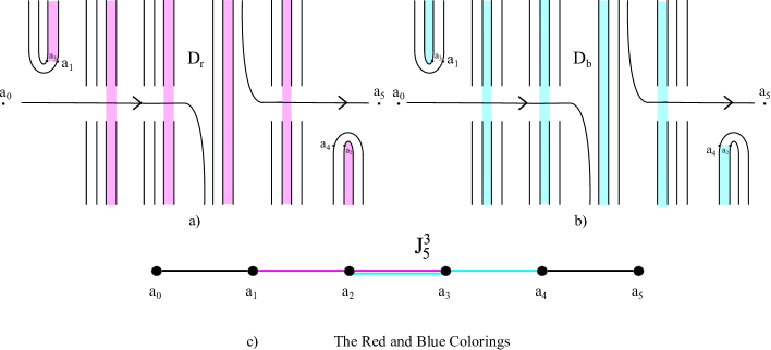 |
Remark 7.4.
These colorings are very helpful for keeping track of both location and orientation. Here is a first application.
Lemma 7.5.
are homotopically trivial.
Proof.
While we already know this result it is useful to see it from the coloring point of view. We prove this for with the argument being similar. Following the red coloring, slide the base of the red bands until they reach ’s top. From there it is apparent that these bands form a parallel cancel pair. See Figure 45. By Lemma 4.6 the support of the undo homotopy is within the union of a neighborhood of the bases and a neighborhood of the parallelism between the bands and the parallelism between the lasso spheres, thus there is no problem with the band linking the lassos.∎
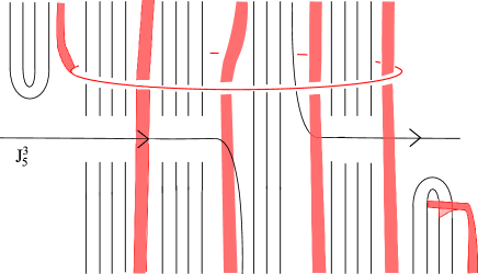 |
Convention 7.6.
We let denote the band and lassos defining , where base appears before base along . are defined analogously. The red coloring and blue colorings allow us to readily deduce which base comes first and to keep track of how a given one is oriented. This in turn enables us to orient the red and blue bands near their bases and then orient their lasso discs as indicated in Figure 43. By Remark 4.5 it suffices to draw only the core of the band provided we also know the orientation of the lasso disc. In what follows usually only the core of the band will be shown in the figures.
Lemma 7.7.
(resp. ) is homotopic to the concatenation of the loops (resp. represented in band lasso form in Figure 46. Each of these loops is homotopically trivial.
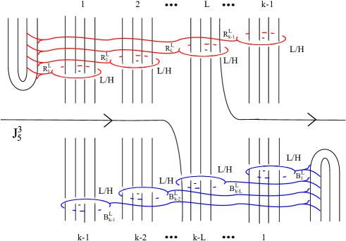 |
Proof.
The principle is that if a lasso encircles two arcs , , then the corresponding spinning about the union can be homotoped into a concatenation of spinnings of the same type (e.g. L/H or positive) about and . The proof that the ’s and ’s are homotopically trivial loops follows as the proof of Lemma 7.5.∎
Notation 7.8.
(resp. ) denotes loop represented by the pair of blue (resp. red) bands and lassos corresponding to linking about the i’th (resp. j’th) local pair of four strands, counted from the right (resp. left).
Remarks 7.9.
i) This notation is chosen, since up to signs/orientations there is a symmetry which takes to such that the bands and lassos defining are taken to those defining . This will induce the skew symmetry mentioned above.
Lemma 7.10.
.
Proof.
The homotopy from to is separable, thus the result follows from bilinearity.∎
Definition 7.11.
Define .
Proposition 7.12.
If and , then )
Proof.
To minimize notation we suppress the superscripts. Figure 47 shows a representative case. Observe that is the concatenation of and where (resp. ) is given by a band lasso pair we call () (resp. () where base( precedes base( on and that is separably homotopic to . The hypotheses on p and q are the conditions such that both the blue and red lassos can slide off of following four of its local strands, so in particular each of and is homotopically trivial. Thus, by bilinearity . Since the support of the undo homotopy of is disjoint from both and its lasso sphere it follows that and hence .
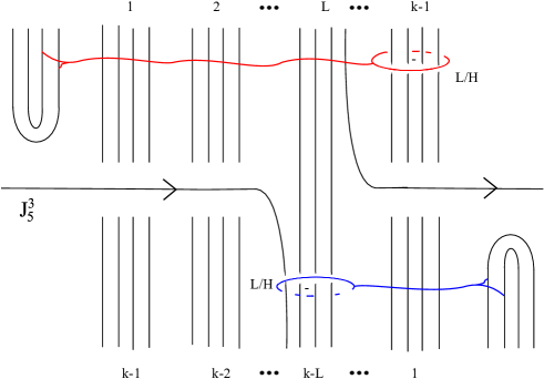 |
To compute slide the red bands so that their bases are near the top of the red coloring and the red lasso discs link near its base. See Figure 48 a). Next, isotope and so that links the cores of the red bands at their branch loci. This is done in two steps. First, use the 4-strand isotopy to isotope off of and link the red bands. Then, isotope to link the bands at their branch loci. Figure 48 b) shows midway through the second step.
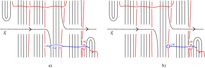 |
We have therefore obtained a as in Definition 4.42. Since the red bases have been moved k times around the and its lasso times around the , following the convention of Definition 4.42, . The blue lasso moves times around to slide off of and then moves times around to link the red bands at their branch loci. Therefore, .
We now compute the sign. Following Remarks 4.43 the sign is determined the parity of how many of the following things deviate from the standard . i) It is of standard type
ii) The blue spinning is
iii) The red spinning is
iv) red band core, blue lasso disc
v) blue band core, red lasso disc Since there are two changes the sign is .∎
Proposition 7.13.
If and or and , then where
if and
if and
if and
if and . if and
if and
if and
if and .
Proof.
To minimize notation we delete the superscript. Case 1: Idea of Proof: As before we reduce to being defined by a single band and lasso. Under the hypothesis only the blue lasso can slide off of by following four strands. To address this, we homotope into a concatenation of and each of whose lassos slides off by following the red coloring. We define and . Each of these has two subcases; and . In the first case the blue and red lassos can slide off of without crashing into each other. In the second case we factor into and each of which can now slide off of without crashing into the red bands and lassos. An argument similar to that of the previous proposition shows that each of is one or two ’s depending on whether subcase 1 or 2 applies.
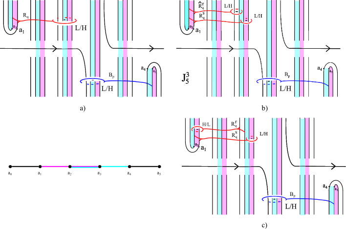 |
Proof of Case 1: is represented by and where the base of appears before that of on . We abuse notation by calling the loop represented by just , since as in the proof of the previous proposition we can use this to compute . Figure 49 a) shows a representative example of a for Case 1. Now homotope into the concatenation of and as in Figure 49 b) and use Lemma 4.4 to reverse the direction of the band and lassos representing to obtain . See Figure 49 c) We use the superscript (resp. ) to denote reversed (resp. standard). Several loops in Figure 49, such as , are represented by two bands and lassos whose bands are branched. For such a pair, the orientation of the lasso disc shown in Figure 49 is for the lasso whose base appears first on . The homotopies of to and to are supported away from both the domain and range support of , thus (resp. ()) is separably homotopic to (resp. ()). Each of the loops and are homotopically trivial for their lassos can be slid off J by following the red coloring. Therefore,
Define and .
Computation of This is very similar to that of the previous proposition. If , then following the red coloring, slide the red lassos to link the core of the blue band near its base and then slide the red bands so that their bases are at the top of the red coloring. Next first slide the blue lasso off of to link the red band cores and then isotope the blue lasso to link the red band cores at their branch loci. The same calculation as in Proposition 7.12 shows that .
If , then slide the blue lasso to just before it crashes into the red lassos and bands. See Figure 50 a). Next homotope into a concatenation of and as in Figure 50 b). The separable homotopy and bilinearity arguments imply that . That follows as in the case. Now is also a with the following changes in comparison with that of . Here we have red band core, blue lasso vs the before, while the other four values determining the sign are the same as those for . Therefore, we have a sign change. The previous argument also shows that . To compute , note that the lasso of is already linking the core of the red bands and a horizontal isotopy moves it to their branch loci while the lasso had to travel an extra times around the to get to the same point. It follows that and hence and so . ∎
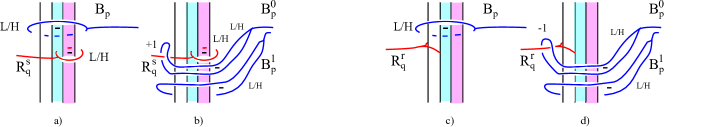 |
Computation of : If , then following the local four strands, isotope the blue lasso off of to link the bands of the red lassos and then further isotope the blue lasso to link these bands at their branch loci. Next, follow the red coloring to isotope the red lassos off of and link the blue band near its base. Finally, isotope the red bands, so that their bases are near the top of the red coloring. This is done in two steps. First isotope so that the bases contain the points and then follow the red coloring from its bottom to near its top. Simultaneously isotope the linking blue lasso to follow along. We now compute the values of this . The blue lasso goes times around the to slide off of and then, in the aggregate, times about the while following the red bands. Therefore, . The red lassos go times around the while in the aggregate the bases go times about the so that . We now compute the sign. i) It is of standard type
ii) The blue spinning is
iii) The red spinning is
iv) red band core, blue lasso disc
v) blue band core, red lasso disc Since there is one sign change from the standard the sign is -. Therefore . If , then slide the blue lasso to just before it crashes into the red bands. See Figure 50 c). Next homotope into a concatenation of and as in Figure 50 d). The separable homotopy and bilinearity arguments imply that . That follows as in the case.
Now is also a . Here as before. To compute , note that the lasso of is already linking the core of the red bands while the lasso had to travel an extra times around the to get to essentially the same point. It follows that . For the sign, note that there is a single change in comparison with the five values computed for . Here red band core, blue lasso disc. It follows that the sign is positive. Therefore, and hence .∎
Case 2: Proof of Case 2: is represented by where the base of appears first. The argument of Case 1 shows that and so we again abuse notation by letting be represented by just . Figure 51 a) shows a representative example of a for Case 2. Note the sign of the lasso disc. In this case is homotopic to a concatenation of and as shown in Figure 51 b). We reverse the direction of the band and lasso representing as in Figure 51 c) to obtain . As before we obtain and define and .
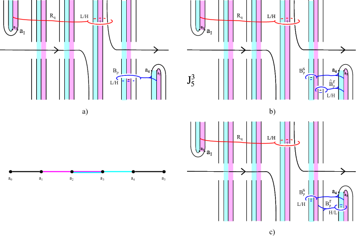 |
Computation of : As in Case 1 this will be one or two ’s depending on whether or not . In both subcases the branched band will be blue, so following Definition 4.42 will be computed using the red band and from the blue bands. With that in mind the calculation follows the method of Case 1. When we have and . To compute the sign note that there are two cancelling changes in comparison with Case 1. Here there is a red/blue switch and also blue band core, red lasso, in comparison with the earlier . Therefore the sign is and .
When , then slide the red lasso to just before it crashes into the blue lassos and bands. See Figure 52 a). Next homotope to a concatenation of and as in Figure 52 b). Here . That follows as in the case. Using that, the method of Case 1 shows that . Therefore, . ∎Computation of : Again there will be one or two ’s depending on whether or not , the branched band will be blue and so will be computed using the red band and from the blue bands. With that in mind the calculation follows the method of Case 1. When we have and . We now compute the sign.
i) It is of type
ii) The blue spinning is
iii) The red spinning is
iv) red band core, blue lasso disc
v) blue band core, red lasso disc There are three changes so that the sign is - and hence .
When , then slide the red lasso to just before it crashes into the blue bands. See Figure 52 c). Next homotope to a concatenation of and as in Figure 52 d). Again .
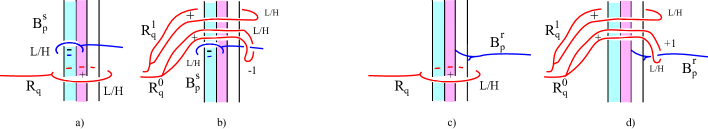 |
That follows as in the case. Using that, the method of Case 1 shows that . Therefore, . ∎
Proposition 7.14.
For and .
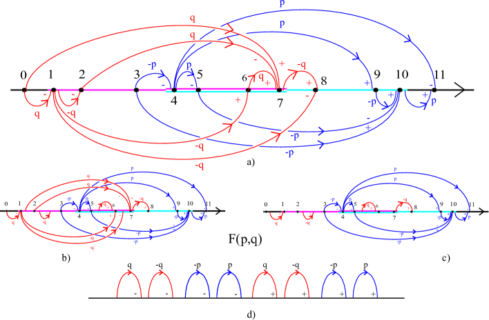 |
Proof.
Again we supress the L’s. Step 1: is represented by the abstract chord diagram pairs of Figure 53 a), b), c) and d).
Proof: A representative is shown in Figure 54 a). Figure 54 b) shows details of neighborhoods of the band bases and lasso discs. Each of the spinnings determined from the four bands and lassos is homotopic to a concatenation of four spinnings of arcs about arcs, via a homotopy that is supported in a small neighborhood of the relevant band and lasso ball. For example, () corresponds to spinning an arc near the point labeled 1 about arcs near the points 0,8,6 and 2. The labeling of the eleven points in the diagram is induced by their ordering in . See Figure 54 c). This data gives rise to the abstract chord diagram of Figure 53 a), where the chords are oriented from the low label to the high one. For each chord we need to compute group elements and signs. For example, gives rise to a spinning where is approximately a horizontal arc in from 1 to 0. If denotes the oriented lasso disc bounded by , then near 0, , so by Lemma 4.5 the oriented chord from 1 to 0 has positive sign. By Lemma 4.4 reversing the direction changes the sign as indicated in Figure 53 a). To compute the group element we concatenate with the arc to obtain an oriented closed loop representing . Since we reversed the direction, the chord in Figure 53 a) is labeled . Note that the colorings inform us that the short arcs between 9,5,3 and 11 as well as the one between 1 and 7 can be homotoped into . It follows that all eight of the chords between these points are labeled .
Applying multiple applications of the Exchange Lemma 4.32 to the red chords gives Figure 53 b). Two applications of the undo homotopy eliminates two pairs of parallel oppositely signed red chords with the same group element, giving Figure 53 c). Similarly, blue exchanges followed by two applications of the undo homotopy gives Figure 53 d).∎Step 2: F(p,q)=0 Proof: Using bilinearity, the class of Figure 53 a) factors into four classes represented by the four chord diagrams , where is the subdiagram consisting of the chords labeled and . The other diagrams are defined similarly. Notice that any diagram can be turned into another by an appropriate sign change of the group elements and exchange moves. By bilinearity factors into four classes represented by the chord diagrams respectively shown in Figures 55 a), b), c), d). The chord diagrams are readily shown to respectively represent and . The chord diagram is obtained from by a chord sliding move. Applying bilinearity factors into where (resp. ) consists of the red chords and the blue chords labeled (resp. ). Now and is readily shown to be equal to . Therefore, and hence
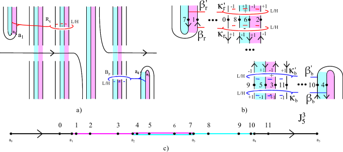 |
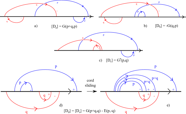 |
Definition 7.15.
Define
.
Here the (resp. , resp. ) denotes blue (resp. red, resp. extra).
Definition 7.16.
Define . Define (resp. ) the matrix with entries (resp. .
Theorem 7.17.
1) If , then
2) If , then
Proof.
1) Fix and . Figure 56 a) shows the points with the red point, denoting , the ’th on the left and the blue point the ’th on the right. Since , the red point is strictly to the left. If (resp. ), then Proposition 7.13 applies for the case (resp. and ). When , then Proposition 7.14 applies.∎
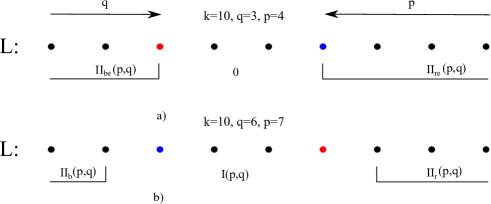 |
Corollary 7.18.
is skew symmetric and hence .
8. Twisting the symmetric
In Definition 6.11 and Construction 6.12 we defined how to twist an implantation and construct its associated 2-parameter family. In particular, we defined the twisted implantations where with the implantations as a special case. In this section we first compute and use that result to show that for the 2-parameter families have linearly independent invariants, thereby completing the proofs of Theorems 3.15 and 8.5.
Theorem 8.1.
, where and .
Proof.
Construction 6.6 showed how to construct the 2-parameter family corresponding to the implantation as a sum of families in band lasso form. Construction 6.12 shows how to modify these families according to the twisting data. In particular, the modification corresponds to locally twisting the bands near where they pass through the lasso discs. Now fix . Recall that we shrunk the bands of these families to obtain families the families and then separably homotoped (resp. ) to a concatenation of . Since the homotopies to the concatenations were supported away from where the strands passed through the blue and red lasso discs it follows that the effect of twisting is to modify the various ’s as in Figure 57, where the case is shown. Note that the four parallel strands undergo a twist in Figure 57 d). We can assume that there is no twisting since these twists can be transferred to the blue bands if and the red bands if and twisting bands by multiples of does not change the homotopy class of the 2-parameter family. It follows that the ’th family of is homotopic to the family as described in Figure 58. The argument of Lemma 7.5 applies without change to these families and hence the result follows by Proposition 4.28.∎
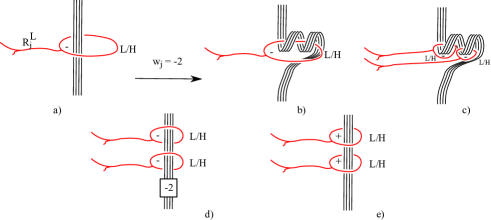 |
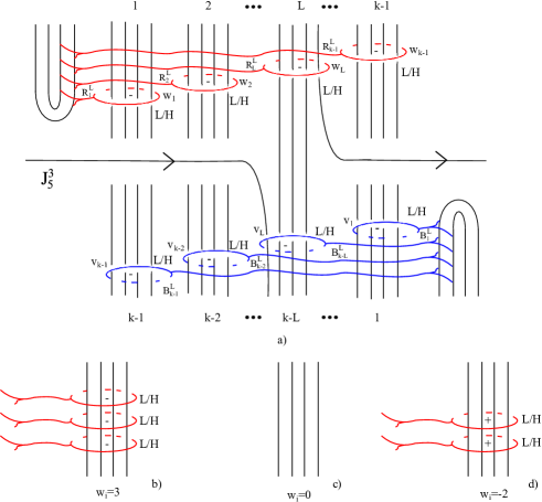 |
Applying to the case of and , i.e. zeros everywhere except for the ’th entry of and ’nd entry of we obtain:
Corollary 8.2.
.
Theorem 8.3.
are linearly independent.
Proof.
Fix . By passing to the quotient of the target of by declaring everything of the form if , then we see that , but in that quotient for . This implies that if we have a finite linear combination of ’s with the largest , then that sum equals zero implies that the coefficient of .∎
Theorem 8.5.
Both and are infinitely generated. In particular, the implantations and their extensions to represent linearly independent elements.
Proof.
That these implantations represent linearly independent elements of follows from Corollary 8.2. Since a diffeomorphism of supported in a can be supported away of it follows that these elements are linearly independent in . Let and be as in Lemma 3.14. Since the ’s represent generators for the image of and by Theorem 7.18, all the ’s are homotopically trivial, it follows that and hence there is an induced homomophism and under this homomorphism the extensions are linearly independent. A similar argument shows that these elements are linearly independent in .∎
Corollary 8.6.
There exist infinitely many distinct knotted non separating 3-spheres in , i.e. there exists infinitely many isotopy classes of 3-spheres that are homotopic to .∎
Corollary 8.7.
There exist infinitely many isotopically distinct fiberings of homotopic to the standard fibering.
Applying Construction 5.9 we obtain the knotted 3-ball by six embedded 0-framed surgeries on , the standard 3-ball in . See Figure 59 b). That figure also shows the conjecturally knotted 3-ball arising from .
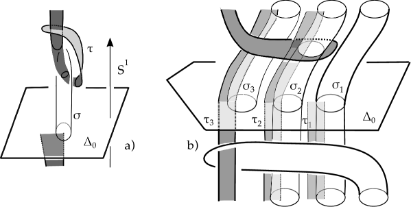 |
| (a) Conjecturally knotted -ball arising from . (b) Knotted -ball arising from |
9. Knotted 3-Balls and the Schönflies Conjecture
In this section we detail the close connection between knotted 3-balls in , and knotted 3-balls in and the relation between the Schönflies conjecture and virtual unknotting of 3-balls.
Definition 9.1.
Let be a 3-ball in . We say that the 3-ball is knotted relative to if and is not isotopic rel to .
In what follows will denote a standard or linear 3-ball as defined in the introduction. It is to be fixed once and for all. Its boundary, the 2-unknot, will be denoted by . Unless said otherwise, 3-balls in will all have boundary equal to and knottedness is relative to . Relative knottedness is essential for by [Ce1] p. 231, [Pa] any two smooth embedded -balls in the interior of a connected -manifold are smoothly ambiently isotopic.
We abuse notation by letting also denote . Its use should be clear from context.
Definition 9.2.
The properly embedded non-separating 3-ball is knotted if it is not properly isotopic to .
Remark 9.3.
Equivalently is knotted if it is properly homotopic to but not properly isotopic to . Since any two non-separating 2-spheres in are isotopic [Gl], [Ha2], we can assume that . By uniqueness of regular neighborhoods we can further assume that coincides with near partial and since , the diffeomorphisms homotopic to id, is connected they have the same parametrization there. Finally, since up to paths in and translations in , [Ha2] it follows that if and are isotopic and already coincide near , then there is an isotopy fixing a neighborhood of the boundary pointwise. By [Ce2], since is connected, has a unique parametrization up to isotopy.
Since is diffeomorphic to the closed complement of the unknot in it follows that we can assume, up to isotopy fixing the boundary pointwise, that all 3-balls with boundary coincide with near . Also, that there exists a uniform neighborhood of such that .
Notation 9.4.
Let be a fixed regular neighborhood of the unknot in , with isotoped to be properly embedded in . Fix a diffeomorphism such that .
The following is immediate.
Proposition 9.5.
induces a 1-1 correspondence between isotopy classes of knotted 3-balls in and knotted 3-balls in .∎
Remark 9.6.
It is important to remember that our correspondence is given by , since by Theorem 3.12 acts transitively on properly embedded 3-balls of .
Theorem 9.7.
If and are properly embedded 3-balls in coinciding near their boundaries, then there exists an orientation preserving diffeomorphism fixing pointwise. Any 3-ball with boundary restricts to a fiber of a fibration of .
Proof.
Theorem 9.8.
induces isomorphisms between the following abelian groups.
i) Isotopy classes of 3-balls in with boundary
ii) isotopy classes of 3-balls in with boundary
iii)
Proof.
Recall that by we mean isotopy classes of diffeomorphisms of fixing a neighborhood of pointwise modulo diffeomorphisms that are supported in a compact 4-ball.
To an element we associate the 3-ball . It’s isotopy class is well defined since up to isotopy. If is a 3-ball with boundary , then by Theorem 9.7 there exists a with . If is another such diffeormorphism and , then . By [Ce2] we can assume that after isotopy pointwise, and then also pointwise. Thus is equivalent to modulo . It follows that there is a 1-1 correspondence between ii) and iii).
Recall that the group structure on 3-balls in to be the one induced from , so is the id and multiplication is given by concatenation. Use to induce the group structure on isotopy classes of 3-balls in with boundary and hence the isomorphism between i) and ii).
Theorem 3.8 implies that these groups are abelian. ∎
Remark 9.9.
Theorem 1.10 of [Ga1] proves the uniqueness of spanning 2-discs in , i.e. two discs with the same boundary are isotopic rel boundary. The existence of knotted 3-balls in , i.e. the non uniqueness of spanning 3-discs in , negatively answers Question 10.13 of [Ga1] for . The second author also conjectured that knotted 3-balls exist [Ga3].
Corollary 9.10.
There exist fiberings of the unknot not isotopic to the linear fibering. The set of isotopy classes of fiberings forms an infinitely generated abelian group.∎
The four dimensional smooth Schönflies conjecture is that smooth 3-spheres in the 4-sphere are smoothly isotopically standard. In 1959 Mazur [Ma1] showed that such spheres are topologically standard. More generally Brown [Br] and Morse [Mo] showed that locally flat 3-spheres in are topologically standard. The corresponding conjecture is known to be true smoothly for all dimensions not equal to four.
The following is essentially stated in [Ga1] as Remark 10.14.
Theorem 9.11.
The following are equivalent:
i) The Schönflies conjecture is true.
ii) For every 3-ball in with , there exists such that the lift of to the -fold cyclic branched cover of , branched over is isotopic to rel .
iii) For every non-separating properly embedded 3-ball in , there exists such that the lift of to the n-fold cyclic cover of is isotopically standard.
Proof.
Let be an unknotted -sphere. If is an embedded 3-sphere that coincides with in a neighborhood of a -disc, then is isotopic to if and only if there exists an isotopy that also fixes a neighborhood of the 3-disc pointwise.
We now show that i) implies ii). Let be the linear 3-ball such that and is a smooth 3-sphere. Let be a 3-ball in that coincides with near . By passing to a sufficiently high odd degree branched cover over we can assume that there are preimages of such that coincides with near , and is a smooth, necessarily unknotted, 3-sphere in . Now is another 3-sphere in . It follows from the previous paragraph that is isotopic rel to and so is isotopic to rel and hence is unknotted.
Now we show that ii) implies i). Let be a 3-sphere in . We can assume that it coincides with the unknotted 3-sphere , constructed above, near the 3-disc . Let be the closed 3-disc in complementary to . By hypothesis, becomes unknotted in a -fold branched cover of branched over , given by . In this cover let be a preimage of , be the preimage of that coincides with near their common boundary, and be the preimages of cyclically ordered about with lying in the region bounded by that contains no other ’s. If is isotopic to via an isotopy supported in , then by composing with we obtain an isotopy between and supported away from and hence one between and . Since the isotopy from to is supported away from it follows that when lifted to the infinite cyclic branched cover the support of the isotopy hits only finitely many preimages of . Thus the original n could have been chosen so that the support of the isotopy is disjoint from some , . Since the region between and (resp. and ) is a relative product, the isotopy can be modified to be supported in .
The equivalence of ii) and iii) follows from Theorem 9.7.∎
Remark 9.12.
An unpublished consequence of [Ma2] due to Barry Mazur and rediscovered in conversations between the second author and Toby Colding is the following. If the Schönflies conjecture is false, then there exists an such that is isotopically non standard even after lifting to any finite sheeted covering of .
Definition 9.13.
We say that the 3-ball is virtually unknotted if it becomes unknotted after lifting to some finite cover of .
Proposition 9.14.
If is the result of finitely many pairwise disjoint barbell implantations each possibly raised to some power in , then for sufficiently large the lift to the n-fold cyclic cover is isotopic to modulo .
Proof.
For sufficiently large is homotopic to the composition of finitely many maps each supported in a 4-ball. ∎
Corollary 9.15.
Every knotted 3-ball arising from finitely many barbell implantations is virtually unknotted. ∎
Proposition 9.16.
For each there exist a barbell whose preimage in the -fold cover is the disjoint union of copies of and hence lifts to a knotted 3-ball in the -fold cover.
Proof.
One readily constructs . The implantation of the preimage is . Since by Theorem 8.3, the result follows.∎
10. More Applications
In the next proposition we list some consequences of Proposition 3.7 and Lemma 3.9. We list the consequences in dimension four, although as we see in the proof, all these statements have high-dimensional analogues.
Theorem 10.1.
-
(1)
, and this is an isomorphism under the concatenation operation. The group is free abelian group of rank two. More generally,
-
(2)
is an abelian group with the concatenation operation. Moreover it contains an infinitely generated free subgroup.
-
(3)
is connected, with containing an infinitely generated free subgroup.
-
(4)
is connected, with containing an infinitely generated free subgroup.
Proof.
(1) As we have seen, when ,
The first non-trivial homotopy group of is known to be , generated by the Haefliger trefoil [Bu2]. In [Bu2] the space is denoted . The first non-trivial homotopy group of is .
(2) Our technique for showing the (families) of diffeomorphisms of are non-trivial factors through the fibration .
(3) See Corollary 3.11, when we have .
(4) There is a homotopy-equivalence [Bu2]
The simplest way to think of this is to consider elements of as smooth embeddings that restricts to the standard inclusion outside of the ball . One can conjugate such embeddings via a stereographic projection map, converting the embeddings to embeddings that are standard on a hemisphere. One can then post-compose such an embedding with an isometry of . We are in the fortunate circumstance where the homotopy-fiber of the map can be identified, and it is the orbits of the -action, acting diagonally on the product.
Thus is a bundle over with fiber . and this group maps isomorphically to the subgroup of index two in , which maps to zero in , so our map is injective. ∎
Remark 10.2.
The first sentence of Conclusion (1) is Theorem 10.4 of [Ga1]. The proof here is different, generalizable and arguably more direct.
Allen Hatcher’s proof of the Smale Conjecture [Ha1] together with his and Ivanov’s work on spaces of incompressible surfaces [HI] has as the consequence that the component of the unknot in the embedding space has the homotopy type of the subspace of great circles, i.e. the unit tangent bundle . From the perspective of the homotopy-equivalence this is equivalent to saying the unknot component of is contractible, .
In dimension four we do not know the full homotopy type of , although there is the recent progress of Watanabe [Wa1] where he shows the rational homotopy groups of do not agree with those of . In this regard, this paper asserts the the analogy to Hatcher and Ivanov’s spaces of incompressible surfaces results [HI] are also false in dimension , in particular contrast with the theorem .
Hatcher and Wagoner [HW] (see Cor. 5.5) have computed the mapping class group of for a range of . Specifically
provided . The Hatcher-Wagoner diffeomorphisms survive the map , as do the diffeomorphisms we prove are isotopically nontrivial.
11. Conjectures and Questions
Conjecture 11.1.
The map induced by isotopy extension has kernal the subgroup with . In particular the implantations and are isotopically nontrivial.
We thank Maggie Miller for bringing to our attention the following question.
Question 11.2.
If is a knotted 3-ball in and , are respectively obtained from , by attaching a small 3-dimensional 1-handle , then is knotted, i.e. is not isotopic rel to ? Does become unknotted after finitely many such stabilizations?
Conjecture 11.3.
For each there exists 3-dimensional genus- handlebodies such that and the set of -compressible simple closed curves in coincides with that of , but is not isotopic to via an isotopy that fixes .
Question 11.4.
i) Determine for . ii) Do all elements become trivial after lifting to the 2-fold cover of .
Remark 11.5.
As already noted Hatcher has determined such groups for and all its elements become trivial passing to 2-fold covers. On the other hand by Proposition 9.16 some elements remain nontrivial when passing to such covers, when .
The following is a restatement of a special case of Lemma 3.9, where as explained there, the isomorphism is given by slicing the embedding. Here notation is as in Theorem 10.1.
Theorem 11.6.
.
Problem 11.7.
Use this to prove or disprove the Schönflies conjecture, e.g. to prove the conjecture show that loops in are homotopically trivial where at discrete times of the homotopy one can do geometric moves corresponding to passing to finite sheeted coverings. Such a move might change the homotopy class and may arise from certain reimbeddings of the loop.
Question 11.8.
Does there exists a barbell whose implantation represents a nontrivial element of ?
12. Appendix: G(p,q) is a Whitehead product
The goal of this section is to prove the following result.
Theorem 12.1.
Let denote the standard oriented properly embedded arc in . Under the homomorphism , then up to sign independent of and , .
Remark 12.2.
While stated for the analogous statement and proof holds for any orientable 4-manifold . In the general case is an oriented properly embedded arc in with , , the basepoint for . In the statement below are paths from to respectively and is defined exactly like except that represent elements of
Theorem 12.3.
Let denote an oriented properly embedded arc in the oriented 4-manifold . Under the homomorphism , then up to sign independent of and , .
Idea of Proof of Theorem 12.1: We are motivated by the mapping space model of Sinha [Si1] that was derived from the work of Goodwillie, Klein and Weiss, e.g. see [GKW]. induces a map which is a map of the 5-ball into . By closing off the boundary facets we will essentially modify this map to an element of which is rationally generated by Whitehead products and under our map, up to sign, is taken to . We close off the boundary facets essentially subject to the constraints of the mapping space model, thus our element of is well defined up to other elements that might be obtained by closing off with the same constraints. An element of modulo those elements is by definition .
Notation 12.4.
denotes the configuration space of distinct ordered -tuples of and denotes the quotient of the Fulton - McPherson compactification as defined in Definition 4.1 of [Si1], though there it is denoted by . In this section and is one of or . For our purposes it suffices to consider the connected component of which is the simplex , so from now on will denote that simplex.
Definition 12.5.
We continue to view as with a geodesic arc through the origin of . We fix an identification of with by and will frequently implicitly identify one with the other. In particular, we abuse notation by having denote the basepoint for both and . Let be disjoint closed intervals in containing in their interiors. We color and blue, red and green respectively. See Figure 60 a).
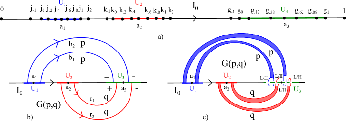 |
We introduced in Figure 19 a) as the bracket . To minimize notation we drop the subscripts. In the next definition we specify , and their end homotopies more precisely and denote the resulting bracket by .
Definition 12.6.
We represent by the chord diagram pair shown in Figure 60 b) and equivalently in band lasso notation in Figure 60 c). The positive chords (resp. negative chords) spin around (resp. ); the corresponding lasso discs intersect at and (resp. and ). The blue (resp. red) chords are called (resp. ) and the spinnings about these chords are respectively supported in the domain in and (resp. and ). The end homotopies for and are the undo homotopies of Definition 12.8. We represent the resulting bracket by .
We define the left shifted (resp. right shifted) mappings (resp. ) as in Figure 61. Here the ends of and (resp. , ) have been isotoped so that they spin about to the left (resp. right) of close to the subinterval (resp. around which (resp. ) already spin.
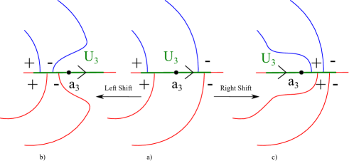 |
Remark 12.7.
The range support of a shift is contained in a small neighborhood of .
We now describe homotopies in of and and their and shifted versions to the constant map to .
Definition 12.8.
The back track homotopy is the homotopy in of a spinning to corresponding to withdrawing the band and lasso and the undo homotopy is defined in Definition 4.7. We now elaborate on these and their variants in our current context.
The blue back track homotopy is the homotopy of to the constant as shown in Figure 62. Each element of the homotopy is a loop of immersed intervals that are embeddings when restricted to , though there may be intersections with . The first part of the homotopy contracts the lasso 3-ball to the arc at the top of the band, so at that moment is a loop that sends an arc to the top of the band and then withdraws it. In a similar manner we define the red back track homotopy as well as the back track homtopies for etc.
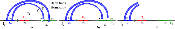 |
The blue undo homotopy , a homotopy in , is defined in Figures 63 a) - g) via continuous transformations of bands, lassos and lasso discs. Figure 63 a) shows . To go from to we zip up the bands to a single one from which two lassos simultaneously emanate as in Figure 63 b). Figure 63 c) is a detail of 34 b). Note that the original lasso discs which are also the lasso discs for and each intersect in one point. To go from to we zip up the lasso discs to obtain a single lasso disc and lasso . Here contains and as subdiscs, the zipping is disjoint from and intersects in two points. See Figure 63 d). To obtain we properly isotope to be disjoint from . See Figure 63 e). This isotopy induces an isotopy of the lasso sphere. The key point is that the lasso spheres remain disjoint from throughout the isotopy, since at each moment the interior of one hemisphere is in the future while the other is in the past. Finally, we withdraw the lasso and bands as in the back track homotopy. In a similar manner we define the red undo homotopy as well as the undo homotopies for , etc.
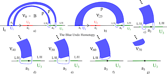 |
In a natural way define the transition homtopy which is a homotopy between the back track and undo homotopies. It’s support is in a small neighborhood of the supports of the undo and back track homotopies. We denote by (resp. ) the transition homotopy for (resp. ).
Summary of Intersections: We now catalogue the intersections and self-intersections of the immersions that arise from evaluating at parameter points the homotopies , as well as their and shifted versions.
1) In the domain is supported in as are all the homotopies of . All homotopies of are homotopies of loops of embeddings when restricted to . is supported in as are all the homotopies of . All homotopies of are homotopies of loops of embeddings when restricted to .
Call a double point of a given map or between two maps of to be of type if it involves the image of a point of intersecting the image of one from .
2) Double points between and are only of type , similarly for their shifted versions. and and their shifted versions are homotopies of loops of embeddings.
3) Double points of a are only of type , similarly for its shifted versions. There are no double points between a and a . Double points of a are only of type , similarly for its shifted versions
4) Double points involving transitional homotopies or their shifted versions are only of type or .
5) Any double point involving an shifted map (resp. shifted map) occurs in (resp. .
Definition 12.9.
Define two open covers of called the standard decompositions as indicated in Figure 64 a).
.
For we define two open covers of called the L-R and - open covers. For the L-R cover, use the standard cover, independent of . Let be very small and as in Figure 63 b). For use the standard decomposition. For define as above and . For , define and .
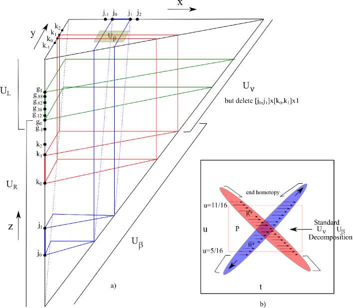 |
Remark 12.10.
contains all the parameters that are both blue and red and contains the parameters corresponding to the end homtopies.
Definition 12.11.
Let denote the 3-ball and . Here points are denoted where , and . Also, unless .
We define . First, define by . Extend to ( as follows. For , according to or , monotonically shift to the left or right. So, if say , then is totally shifted to the left. For it is somewhere between the right and the left i.e. is partially shifted. Next, for homotope to according to whether it is in or . I.e. if (resp. the back track (resp. undo) homotopy is used. In the transition homotopy is used.
Definition 12.12.
For let denote the retraction which fixes pointwise and let the retraction to . Letting we obtain . Let be a proper immersion supported in the domain on such that and are embeddings. Let and . Let be the constant speed path in I from to with and similarly defined. We say that is -ready if for all are pairwise disjoint.
Lemma 12.13.
If is embedded, then any is -ready.∎
Notation 12.14.
In what follows if , then denotes the closed interval, possibly a point, between and or and .
Proposition 12.15.
If , then is ready for all .
Proof.
Case 1: .
Proof of Case 1: Let and let denote . If for some , , then since these are unit speed paths with and . Therefore, either and or and . Similar statements hold for and . Thus it suffices to show that there are no intersections involving two of or .
We first show that there is no such intersection involving a . Recall that . If , then no is involved with a intersection. Since then cannot be involved with a intersection. If , then again cannot be involved with a intersection. If , then , so cannot be involved with a intersection. If , then so cannot be involved with a intersection. If , then so there are no intersections and since , cannot be involved with a intersection.
It remains to show that there is no intersection involving both a and an . If , then and hence is not involved with a intersection. If , then so is not involved with intersections. If , then so are and and hence so cannot be involved with a intersection. If , then , so cannot be involved with a intersection. If , then neither is . Therefore if and , then cannot be involved with a intersection. If and , then . Being in it follows that and hence which implies that they cannot be involved in a intersection. ∎
Case 2: . Proof of Case 2 Here for or . We will assume the case of , the other case being similar. Hence it suffices to show that there are no intersections. Such intersections are ruled out by the argument of Case 1.∎
Definition 12.16.
Define by
Definition 12.17.
Define , the -cohorizontal space and for , the s-cohorizontal space. Let be the coordinate functions for . Call a point of (resp. )) a blue cohorizontal (resp. red cohorizontal) point.
Definition 12.18.
As in Definition 4.21, give rise to . Let and denote the parameter supports for and , which by convention lie in the blue and red regions of Figure 64 b). Let denote . By reparametrizing we will assume that for each , , where is very small and is contained in the neighborhood of the arc from to . Similar statements hold for , where the domain support of is denoted and is contained in the neighborhood of the arc from to . Define the blue slab (resp. red slab) such that (resp. ). Define . Let denote the projection of to , the projection to the first factor, the projection to the second factor and the projection to the factor. Define to be the projection of .
Proposition 12.19.
(the blue sphere) and (the red sphere) are disjoint 2-spheres whose union is the standard Hopf link in . If is a path from to (resp. ), then (resp. ) represents the class (resp. ).
Remark 12.20.
Note that and
Proof.
Let and . The Proposition follows from the following seven steps.
Step 1: If where , then either or . Also either
i) , in which case is a partially shifted or
ii) , in which case is obtained from either a shifted or partially shifted or its image under the undo homotopy.
Proof of Step 1: By construction, the lasso spheres of and and those of the undo homotopy project under to their lasso discs. The and lasso discs are disjoint from and their lasso discs and those of the undo homotopies are disjoint when fully shifted left or right. It follows that if , then . When a similar argument proves shows that .∎
Step 2: We can assume the following.
i) Under the left shift the (resp. ) lasso disc intersects when (resp. ) and under the right shift the (resp. ) lasso disc intersects when (resp. ).
ii) Viewing as a map , then the projection of to . Similarly the projection of equals .
iii) Viewing as a map where and is the constant map to , then the projection of to consists of two, one or zero points. Here denotes . In the former case the lower (resp. higher) point in is monotonically increasing (resp. decreasing) and equals when there is exactly one point. An analogous statement holds for .
iv) The lasso discs of intersect in two, one or zero points. When there are two points the lower (resp. higher) point in is monotonically increasing (resp. decreasing) in . An analogous statement holds for .
v) Near and . ∎
Step 3: is independent of and is when , is one point when , is two points when and an interval when . Furthermore,
i) If , then
ii) If , then , where
iii) if , then , where is non increasing and
iv) if , then , where
v) if , then , where .
An analogous statement holds for . ∎
Step 4: .
Proof of Step 4: If and , then when restricted to one of or and hence Step 4 follows. Now suppose that . If , then apply Step 1 to conclude . If , then (resp. ) implies (resp. ). If , then and hence by Step 2, while . If , then and hence by Step 2, while . If , then either or or . In all three cases at least one of or holds and hence .∎
Step 5: For , is independent of and equal to a Hopf link. Also and .
Proof of Step 5: The invariance and the Hopf link property follow by Steps 2 and 3. Figure 65 b) shows , a Hopf link within the blue and red slabs. If , then and hence . If , then and hence . ∎
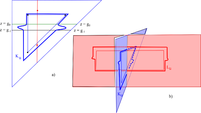 |
Step 6: The surface is a disc that after proper isotopy in projects under to a spanning disc for . Analogous statements hold for , and . Proof of Step 6: This is a long but routine exercise along the lines of Step 3. Here one computes the various intersections of with each and shows that after a small proper isotopy to eliminate arcs projecting to points, the projection of to is embedded. ∎
Step 7: If is a path from to (resp. ), then (resp. ) represents the class (resp. )). Proof of Step 7: Step 4 follows from the definition of . Here we view as the basepoint. ∎
Proof of Theorem 12.1: We will show that there is a homotopy of to supported away from such that throughout the homotopy and each of the homotopies of and are supported away from . Furthermore, there exists disjoint regular neighborhoods such that off of and off of . Since each of and have trivial normal bundles and the restriction of and to the fibers of and project to degree maps to , the homotopy can be chosen so that the restriction of to a fiber is a whisker from to that goes times around the followed by the standard quotient map of the 3-ball to . The analogous statement holds for where the whisker starts at and goes q times about . It follows that we have, up to sign independent of and , the Whitehead product
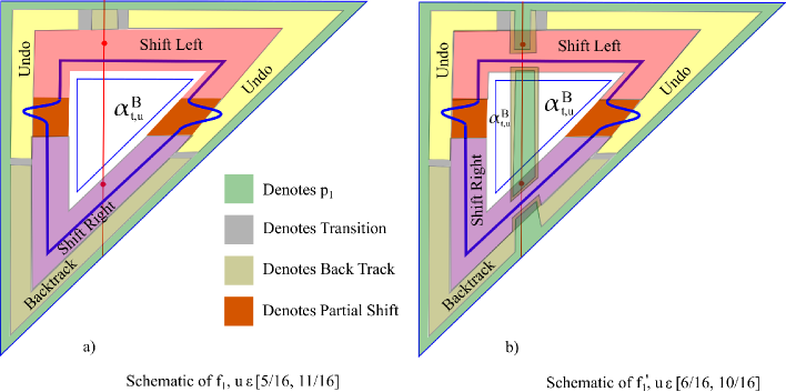 |
The mapping , is schematically shown in Figure 66 a). The closed subset corresponding to is the closed region interior to the blue triangle. We denote that region by since in that region . Since near the boundary of , that region is denoted by . In the collar, is modified by the left, right, undo and backtrack homotopies as indicated in the diagram. A similar discussion holds for , though in that case the diagram is of a square.
We next homotope to so that in the region is defined as in Figure 66 b). Here we modify or its partially left or right shifted versions by the blue back track homotopy. Note that the homotopy is done away from where a blue lasso disc crosses under left or right shifting and hence the homotopy is supported away from . In a similar manner we homotope to . Since for any the corresponding blue bands and lasso discs are disjoint from the red ones, there is no nontrivial intersection between the images of and under the homotopy. Note that the support of is now a regular neighborhood of disjoint from a regular neighborhood of which is the support of . ∎
References
- [AS] G. Arone & M. Szymik, Spaces of knotted circles and exotic smooth structures,arXiv: 1909.00978.
- [Br] M. Brown, A proof of the generalized Schoenflies theorem, Bull. Amer. Math. Soc. 66 (1960), 74–76.
- [Bu1] R. Budney Little cubes and long knots, Topology 46 (2007) 1–27.
- [Bu2] R. Budney, A family of embedding spaces, Geometry & Topology Monographs, 13 (2008) 41–83.
- [BCSS] R. Budney, J. Conant, K. Scannell, D. Sinha, New perspectives on self-linking, Adv. Math. 191 (2005) 78–113.
- [BG2] R. Budney & D. Gabai, Scanning diffeomorphisms, in preparation.
- [Ce1] J. Cerf, Topologie de certains espaces de plongements, Bull. Soc. Math. France, 89 (1961), 227–380.
- [Ce2] J. Cerf, Sur les Diffeomorphismes de la Sphere de Dimension Trois , Springer Lecture Notes, 53 (1968).
- [Ce3] J. Cerf, La stratication naturelle des espaces de fonctions differentiables reels et le theoreme de la pseudo-isotopie, Inst. Hautes Etudes Sci. Publ. Math. 39 (1970), 5–173.
- [CG] F. Cohen, S. Gitler, On loop spaces of configuration spaces, T. AMS 354 No. 5, 1705–1748.
- [Da] J. P. Dax, Etude homotopique des espaces de plongements, Ann. Sci. Ecole Norm. Sup. (4) 5 (1972), 303–377.
- [E2] R. D. Edwards, The 4-Dimensional Light Bulb Theorem (after David Gabai), ArXiv:1709.04306.
- [Fr] M. Freedman, The disk theorem for four-dimensional manifolds, Proc. Int. Cong. Math., (1983), 647–665.
- [FQ] M. Freedman & F. Quinn, Topology of 4-manifolds, Princeton Mathematical Series, 39, Princeton University Press, Princeton, NJ, 1990.
- [Ga1] D. Gabai, The four dimensional light bulb theorem, J. AMS 33 (2020), 609–652.
- [Ga2] D. Gabai, Self-Referential discs and the light bulb lemma, to appear, Comment. Math. Helv.
- [Ga3] D. Gabai, OIST Lecture, January 23, 2019.
- [Gl] H. Gluck, The embedding of two-spheres in four-spheres, B. AMS, 67(1961), 586–589.
- [GKW] T. Goodwillie, J. Klein & M. Weiss, Spaces of Smooth Embeddings, Disjunction and Surgery, Surveys on Surgery Theory, vol. 2, Ann. of Math. Stud., 149, Princeton, 2001, pp. 221–284.
- [GW2] T. Goodwillie, M. Weiss, Embeddings from the point of view of immersion theory. Part II. Geom. Topol. Vol 3, No. 1 (1999) 103–118.
- [HW] A. Hatcher, The second obstruction for pseudo-isotopies, Astérisque, tome 6 (1973). Part II.
- [Ha1] A. Hatcher A proof of the Smale conjecture, Ann. of Math. (2) 117 (1983), 553–607.
- [Ha2] A. Hatcher, On the diffeomorphism group of , Proc. Amer. Math. Soc. 83 (1981), no. 2, 427–430. Also, 2003 revision available from http://pi.math.cornell.edu/~hatcher/.
- [Ha3] A. Hatcher, The second obstruction for pseudo-isotopies, Astérisque, tome 6 (1973). Part II.
- [HI] A. Hatcher, Homeomorphisms of sufficiently large -irreducible 3-manifolds, Topology 15 Issue 4 (1974) pg. 343–347.
- [Hir] M. Hirsch, Differential Topology, Springer GTM 33 (1976).
- [Ki] R. Kirby, Problems in low dimensional manifold theory, Proc. Sympos. Pure Math., 32 Part 2 (1978), 273–312.
- [KM] M. Klug & M. Miller, Concordance of surfaces in 4-manifolds and the Freedman-Quinn invariant, preprint.
- [Ko1] D. Kosanovic, A geometric approach to the embedding calculus knot invariants, 2020 thesis, Rheinischen Friedrich-Wilhelms-Universitat Bonn.
- [Ko2] D. Kosanovic, Embedding calculus and grope cobordism of knots, ArXiv preprint.
- [La] F. Laudenbach, Sur Les 2-spheres d’une variete de dimension 3, Ann. of Math., (2) 97 (1973), 57–81.
- [Lev] J. Levine, Inertia Groups of Manifolds and Diffeomorphisms of Spheres, American Journal of Mathematics Vol 92, No. 1 (Jan. 1970) 243–258.
- [Ma1] B. Mazur, On embeddings of spheres, Bull. Amer. Math. Soc. 65 (1959), 59–65.
- [Ma2] B. Mazur, personal communication.
- [Mi] J. Milnor, Lectures on the h-cobordism theorem, Princeton University Press, Princeton NJ, 1965.
- [MM] J. Milnor, J. Moore, On the structure of Hopf algebras, Ann. Math. 81 (2): 211–264.
- [Mor] S. Moriya, Models for knot spaces and Atiyah duality, preprint.
- [Mo] M. Morse, A reduction of the Schoenflies extension problem, Bull. Amer. Math. Soc. 66 (1960), 113–115.
- [MV] B. Munson, I. Volić. Cubical Homotopy Theory. Cambdridge University Press.
- [Pa] R. Palais, Extending diffeomorphisms, Proc. Amer. Math. Soc. 11 (1960), 274–277.
- [Po] M. Polyak, Invariants of immersions via homology intersections, (in preparation).
- [PV] M. Polyak, O. Viro, Gauss Diagrams for Formulas of Vassiliev Invariants, IMRN (1994), No. 11.
- [ST] R. Schneiderman & P. Teichner, Homotopy versus Isotopy: Spheres with duals in 4-manifolds, arXiv:1904.12350.
- [Sch] H. Schwartz, Equivalent non-isotopic spheres in 4-manifolds, J. Topol. 12 (2019), 1396–1412
- [Si1] D. Sinha, The topology of the space of knots: Cosimplicial models, American J. Math., 131 (2009), 945–980.
- [Si2] D. Sinha, Manifold-theoretic compactifications of configuration spaces, Selecta Math. (N.S.) 10 (2004), no.3, 391–428.
- [Sm1] S. Smale, A classification of immersions of the two-sphere, Trans. AMS (1957), 281–290.
- [Sm2] S. Smale, The classification of immersions of spheres in Euclidean spaces, Ann. of Math. (2) 69 (1959), 327–344.
- [Sm3] S. Smale, Diffeomorphisms of the 2-Sphere, Proc. AMS, 10 (1959), 621–626.
- [Sp] D. Spring, The golden age of immersion theory in topology, B. AMS 42 (2005), 163–180.
- [St] R. Stong, Uniqueness of -negligible embeddings in 4-manifolds: A correction to theorem 10.5 of Freedman and Quinn, Topology, 32 (1993) 677–699.
- [Wa1] T. Watanabe, Some exotic nontrivial elements of the rational homotopy groups of , arXiv:1812.02448.
- [Wa2] T. Watanabe, Theta-graph and diffeomorphisms of some 4-manifolds, arXiv:2005.09545.