Scale-wise Convolution for Image Restoration

Abstract

While scale-invariant modeling has substantially boosted the performance of visual recognition tasks, it remains largely under-explored in deep networks based image restoration. Naively applying those scale-invariant techniques (e.g., multi-scale testing, random-scale data augmentation) to image restoration tasks usually leads to inferior performance. In this paper, we show that properly modeling scale-invariance into neural networks can bring significant benefits to image restoration performance. Inspired from spatial-wise convolution for shift-invariance, “scale-wise convolution” is proposed to convolve across multiple scales for scale-invariance. In our scale-wise convolutional network (SCN), we first map the input image to the feature space and then build a feature pyramid representation via bi-linear down-scaling progressively. The feature pyramid is then passed to a residual network with scale-wise convolutions. The proposed scale-wise convolution learns to dynamically activate and aggregate features from different input scales in each residual building block, in order to exploit contextual information on multiple scales. In experiments, we compare the restoration accuracy and parameter efficiency among our model and many different variants of multi-scale neural networks. The proposed network with scale-wise convolution achieves superior performance in multiple image restoration tasks including image super-resolution, image denoising and image compression artifacts removal. Code and models are available at: https://github.com/ychfan/scn˙sr.

1 Introduction

The exploitation of scale-invariance in computer vision and image processing has greatly benefited feature engineering (?), image classification (?), object detection (?; ?; ?; ?; ?), semantic segmentation (?; ?) and the training of convolutional neural networks (?; ?). For example, Lowe proposed the scale-invariant features (SIFT) (?) that are consistent across a substantial range of affine distortion. Due to its robustness, the SIFT features have been shown undeniably successful and ubiquitously used for image matching, image classification, object detection and many others computer vision tasks. More recently, the importance of scale-invariance is demonstrated in object detection using convolutional neural networks (?), which is further improved by an efficient multi-scale training method (?) of object detectors.

While modeling scale-invariance has greatly improved visual recognition performance, few efforts have succeeded in utilizing scale-invariant features for image restoration tasks based on convolutional neural networks. For example, random-scale data augmentation during training and multi-scale testing are proven beneficial to a wide range of image recognition problems like classification (?) and detection (?). However, naively applying those techniques usually lead to worse performance for image restoration like super-resolution. It is likely due to the fact that, unlike image recognition problems, the performance of low-level image restoration tasks is very sensitive to naive scaling of input images. Is modeling scale-invariance unnecessary for image restoration tasks?

In this work, we demonstrate that properly modeling scale-invariance into convolutional neural networks can bring significant gain for image restoration tasks. We draw inspiration from spatial-wise convolution for shift-invariance, and propose the “scale-wise convolution” that is designed to convolve across multiple scales to achieve scale-invariance. In our scale-wise convolutional network (SCN), we first map the input image to the feature space and then build a feature pyramid representation via bi-linear down-scaling progressively. Based on the feature pyramid, we apply the same function (several shared layers) to process different scales and aggregate the neighborhoods. After several residual blocks with scale-wise convolutions, we take the feature output of the largest scale and predict the results with a linear convolution. The proposed scale-wise convolution learns to dynamically activate and aggregate features from different input scales in each residual building block, in order to exploit contextual information on multiple scales.

We compare our proposed network to several multi-scale convolutional networks with different design choices (shared or un-shared weights, different layer connectivity, etc). We show in our experiments that these multi-scale convolutional networks are inferior than our proposed scale-wise convolutional network. We also study the way of feature fusing across different scales: i.e., (1) convolution and deconvolution with stride, (2) average pooling down-sampling and nearest neighbour up-sampling, and (3) bilinear re-sampling (both down-sampling and up-sampling). We further study the number of scales and the scale factor in our scale-wise convolutional networks and analyze their performances.

To demonstrate the effectiveness of our proposed scale-wise convolutional networks, we conduct extensive experiments on image super-resolution, denoising and compression artifacts removal. Our experiments reveal that: (1) Multi-scale models significantly improve the performance compared with single-scale models. (2) Scale-wise convolution for cross-scale modeling is more parameter-efficient than general multi-scale models, and achieves better efficiency-accuracy trade-offs. (3) Scale-wise convolution benefits from more scales in feature pyramid and proper scaling ratios in-between. Moreover, our proposed SCN can achieve superior results to state-of-the-art methods with even fewer parameters on image super-resolution, denoising and compression artifacts removal.

2 Related Work

2.1 Scale-Invariant Modeling in Visual Perception

The prior of scale-invariance in image processing has motivated many deep neural network architectures and models. For example, a scale-invariant convolutional neural network (SiCNN) proposed by (?) is designed to incorporate multi-scale feature exaction and classification into the multi-column architecture. These columns share a same set of weights which are transformed for different scales. SiCNN improves the performance of image classification by learning the feature in different scales in different columns. Multi-scale architectures like U-Net (?) and SegNet (?) incorporate multiple scales in different network staged and inter-connects them, which are proven to have higher performance on image segmentation tasks. Feature Pyramid Network (?) proposed a top-down architecture with lateral connections for building high-level semantic feature maps at all scales. Moreover, during the training and testing of deep neural networks, multiple scales can also be useful for a wide range of applications like classification and detection.

2.2 Multi-Scale Architectures in Image Restoration

Several approaches have explored involving multiple scales into neural network architecture for image restoration tasks. The Dual-State Recurrent Network (DSRN) (?) proposed a neural network to jointly utilize signals on both low-resolution scale and high-resolution scale for image super-resolution. Specifically, recurrent signals in DSRN are exchanged between these two scales in both directions via delayed feedback. The Deep Back-Projection Networks (?) exploited multiple iterative up-sampling and down-sampling layers, which provides an error feedback mechanism for projection errors at each stage of image super-resolution. Balanced two-stage network (?) is decoupled into scales along layers. Multi-scale residual network (MSRN) is proposed to fully exploit the image features (?), in which the convolution kernels of different sizes can adaptively detect the image features in different scales.

2.3 Weight Sharing in Image Restoration

For image restoration tasks, the receptive field of a convolutional network has a critical role as it determines the amount of contextual information that can be used for prediction. However, naively increasing the number of layers leads to computationally expensive models with low parameter efficiency. To make a model compact, recursive neural networks (?; ?) are proposed by sharing weights repeatedly among different recurrent stages. The recurrent architecture has also been used in  (?; ?).

3 Scale-wise Convolutional Networks

In this section, we introduce our approach in the following manner. We first describe the scale-wise convolution operator and discuss its properties in details. Then the scale-wise convolutional networks are developed based on repeatedly constructing residual blocks with scale-wise convolution. Finally we discuss a number of design choices and construct several multi-scale network variants as our baselines.

3.1 Scale-wise Convolution

We propose the scale-wise convolution operator that convolves features along the scale dimension from a multi-scale feature pyramid. Figure 1 visually illustrates the idea of “convolution” across scales.

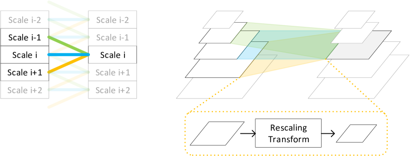
Figure 1: Illustration of scale-wise convolution. Left: projected view of scale-wise convolution over features in different scales. Right: scale-wise convolution as sum of features from neighbour scales transformed by $f_{i}$.

Formally, the scale-wise convolution $\mathcal{F}$ takes a multi-scale feature pyramid $\boldsymbol{X}^{l}=\{\boldsymbol{x}_{s}^{l}\}_{s=1}^{N}$ from layer $l$ with multiple scales from $1$ to $N$, and generates the next feature pyramid with the same size $\boldsymbol{X}^{l+1}=\mathcal{F}(\boldsymbol{X}^{l})$ by “convolution” across scales. The output feature $\boldsymbol{x}_{s}^{l+1}$ is transformed from features of previous neighbouring scales $\{\boldsymbol{x}_{s-k}^{l},\dots,\boldsymbol{x}_{s}^{l},\dots,\boldsymbol{x}_{s+k}^{l}\}$. Specifically, the output of scale-wise convolution with kernel size $2k+1$ for layer $l+1$ and scale $s$ is computed as

$$\boldsymbol{x}_{s}^{l+1}=\sum_{i=-k}^{k}f_{i}(\boldsymbol{x}_{s+i}^{l})=\sum_{i=-k}^{k}h_{i}\circ g_{i}(\boldsymbol{x}_{s+i}^{l}),$$

where $g_{i}$ is a spatial convolution to transform features $\boldsymbol{x}_{s+i}$ and $h_{i}$ is an operator to adjust height and width of features towards target scale $s$. The scale-wise convolution acts as a sliding window to perform the same transformation along the scale dimension. Such a convolution operation is designed to extract information from features on multiple scales in a compact manner, and is able to better capture scale-invariance than naive multi-scale or single-scale networks, which will be shown in our experiments.

To reduce additional parameters of scale-wise convolution compared with legacy spatial one, the operation $f_{i}$ can be further decomposed as

$$f_{i}=h_{i}\circ g_{i}=h_{i}\circ q_{i}\circ p,$$

where $p$ is a spatial convolution with shared kernels across scales and $q_{i}$ is a point-wise convolution for scale-specific feature transformation. Hence, the only additional parameters in $q_{i}$ are negligible.

There are multiple candidate operations to achieve features from different scales, including (1) convolution and deconvolution with stride, (2) average pooling and nearest neighbour up-scaling, (3) bilinear re-scaling for both down-scaling and up-scaling. In convolution, deconvolution and average pooling, the ratio of up-scaling and down-scaling is controlled by the striding, which is an integer number (e.g., stride=2). In comparison, the bilinear re-scaling approach are more flexible since it can be applied to arbitrary scale ratios. We will also show in experiments that the bilinear re-scaling achieves slightly better performance. Therefore, we use bilinear re-scaling as our feature fusing operator by default.

Comparison to Spatial Convolution.

Regular spatial convolution explores context information from neighbouring pixels. In a convolutional neural network (assuming no pooling operations), the receptive field grows linearly by the increase of the convolutional layers. Our proposed scale-wise convolution is built on a multi-scale feature pyramid. It mutually exchanges cross-scale information in every layer, and the spatial receptive field grows exponentially because the information of smaller scales are progressively fused into the current scale.

3.2 Scale-wise Convolutional Networks for Image Restoration

The proposed SCN is built upon widely-activated residual networks for image super-resolution (?; ?; ?), by adding multi-scale features and scale-wise convolutions in residual blocks.

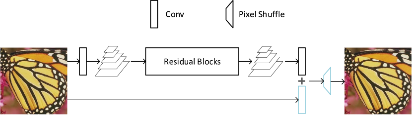
Figure 2: Overview of scale-wise convolutional networks for image restoration. Input image is first transformed into feature pyramid, then processed by multiple residual blocks with scale-wise convolution inside, finally feature pyramid is converted into target scale and fused with global skipped features.

Unified Architecture for Image Restoration.

The proposed SCN has multiple cascaded residual blocks and a global skip path way, as shown in Figure 2. Many low-level image restoration problems can be treated as dense pixel prediction task and share the same unified network structure. For image super-resolution, additional pixel shuffle layer and spatial convolution layer for global skip connection (blue modules in Figure 2) are required to map low-resolution input to high-resolution counterpart. For the task of image denoising and JPEG image compression artifacts removal, the additional layers in blue are removed.

Multi-Scale Feature Pyramid.

The scale-wise convolution is performed on a consecutive multi-scale feature pyramid. In SCN, the initial feature pyramid is built from a linearly transformed features of original images (i.e., mapping input image to feature space with a simple spatial convolution layer). As shown in Figure 2, the feature maps after the first spatial convolution layer are progressively down-sampled using the re-scaling operations (bi-linear re-scaling by default). After multiple scale-wise convolutional residual blocks, each feature scale will have the information from distant scales and a exponentially increased spatial receptive field.

The scaling factor for building feature pyramid needs to be chosen carefully. When factor is close to one, features from adjacent scales will be similar and redundant. Meanwhile, receptive field growth will also degrade from exponential to linear by binomial expansion. When factor is close to zero, the number of scales will be limited.

Figure 3: Illustration of multi-scale network architectures.

Residual Blocks with Scale-wise Convolution.

Based on the feature pyramid, we apply the same function (i.e., several shared layers) to process different scales. Each residual block has a spatial convolution layer for expanding features, a ReLU activation layer and another spatial convolution layer for mapping feature back to original feature size. Afterwards we aggregate the neighbouring scales, as shown in Figure 1. The proposed scale-wise convolution learns to dynamically activate and aggregate features from different input scales in each residual building block.

Widely-activated residual networks (?) with wider features before ReLU activation achieve significantly better performance for image and video super-resolution, with the same parameters and computational budgets. The resulted residual network has a slim identity mapping pathway with wider channels before activation in each residual block. The efficiency of wide activation could further make our SCN compact. Moreover, to fully utilize the benefits of wide activation, we put up-scaling / down-scaling after the second spatial-wise convolution, where the channel numbers have been reduced. It speeds up the running time of our SCN.

Comparison to Multi-Scale Architectures.

Our proposed SCN, at the first glance, is similar to multi-scale neural networks. However, they are fundamentally different in two aspects.

First, the scale-wise convolution applies same weights to different scales, while other multi-scale networks usually aggregate features in difference scales with specific parameters. For example, U-Net style (?) models in Figure 3 progressively down-sample features through explicit stages with multiple network layers in encoder and linearly composite multi-scale features by skip connections in decoder. Moreover, our proposed scale-wise convolution also adapts a unified operator to fuse between different scales and thus is more compact.

Second, the proposed scale-wise convolution aggregates multi-scale features gradually and locally, while other multi-scale networks fuse features at specific layers. For example, PSPNet style (?) models in Figure 3 independently execute over scales and combine multi-scale features in the final layers. The scale-wise convolution fully utilizes the similarity prior of images across scales and is more robust to scale variance. Thus, the proposed operator can be viewed as “convolution” across scales.

Our experiments show that the proposed SCN achieved better performance than previous multi-scale architectures.

4 Experimental Results

We performance our experiments on image super-resolution, denoising and compression artifact removal to show the significance of our proposed SCN for image restoration.

4.1 Experimental Settings

Dataset.

Multiple datasets are used for different image restoration tasks.

For image super-resolution, models are trained on DIV2K (?) dataset with 800 high resolution images since the dataset is relatively large and contains high-quality (2K resolution) images. The default splits of DIV2K dataset consist 800 training images and 100 validation images. The benchmark evaluation sets include Set5 (?), Set14 (?), BSD100 (?) and Urban100 (?) with three upscaling factors: x2, x3 and x4.

For image denoising, we use Berkeley Segmentation Dataset (BSD) (?) 200 training and 200 testing images for training purpose, as (?). The benchmark evaluation sets are Set12, BSD64 (?) and Urban100 (?) with noise level of 15, 25, 50.

For compression artifacts removal, we use 91 images in (?) and 200 training images in (?) for training. The benchmark evaluation sets are LIVE1 and Classic5 with JPEG compression quality 10, 20, 30 and 40.

Training Setting.

Experiments are conducted in patch-based images and their degraded counterparts. Data augmentation including flipping and rotation are performed online during training, and Gaussian noise for image denoising tasks is also online sampled. 1000 patches randomly sample per image and per epoch, and 40 epochs in total. All models are trained with L1 distance through ADAM optimizer, and learning rate starts from 0.001 and halves every 3 epochs after the 25th. We use deep models with 8 residual blocks, 32 residual units and 4x width multiplier for most experiments, and 64 blocks and 64 units for super-resolution benchmarks.

4.2 Main Results

In this part, we compare our models with the state-of-the-art methods on image super-resolution, image denoising and image compression artifact removal. The results are shown in Table 1 (Single Image Super-Resolution), Table 2 (Image Denoising) and Table 3 (Image Compression Artifact Removal).

Image super-resolution.

We compare our SCN with state-of-the-art single image super-resolution methods: A+ (?), SRCNN (?), VDSR (?), EDSR (?), WDSR (?). Self-ensemble strategy is also used to further improve our SCN, which we denote as SCN+.

As shown in Table 1, our proposed SCN and SCN+ achieves best results on all benchmark dataset and across all three upscaling factors. It indicates that properly modeling scale-invariance into neural networks, specifically the scale-wise convolution, can bring significant benefits to image super-resolution.

Furthermore, we visually compare our super-resolved images with other baseline methods. As shown in the Figure 4, our method produces higher quality images (for example, sharper edges) than our baseline methods: SRCNN (?), FSRCNN (?), VDSR (?), LapSRN (?), MemNet (?) and EDSR (?).

Table 1: Public image super-resolution benchmark results and DIV2K validation results in PSNR / SSIM. Red indicates the best performance and blue indicates the second best. $+$ indicates results with self-ensemble.

Dataset Scale Bicubic A+ SRCNN VDSR EDSR WDSR SCN SCN+ $\times 2$ 33.66 / 0.9299 36.54 / 0.9544 36.66 / 0.9542 37.53 / 0.9587 37.99 / 0.9604 38.10 / 0.9608 38.18 / 0.9614 38.29 / 0.9616 Set5 $\times 3$ 30.39 / 0.8682 32.58 / 0.9088 32.75 / 0.9090 33.66 / 0.9213 34.37 / 0.9270 34.48 / 0.9279 34.60 / 0.9295 34.75 / 0.9301 $\times 4$ 28.42 / 0.8104 30.28 / 0.8603 30.48 / 0.8628 31.35 / 0.8838 32.09 / 0.8938 32.27 / 0.8963 32.39 / 0.8981 32.59 / 0.9000 $\times 2$ 30.24 / 0.8688 32.28 / 0.9056 32.42 / 0.9063 33.03 / 0.9124 33.57 / 0.9175 33.72 / 0.9182 33.99 / 0.9208 34.14 / 0.9218 Set14 $\times 3$ 27.55 / 0.7742 29.13 / 0.8188 29.28 / 0.8209 29.77 / 0.8314 30.28 / 0.8418 30.39 / 0.8434 30.50 / 0.8467 30.62 / 0.8483 $\times 4$ 26.00 / 0.7027 27.32 / 0.7491 27.49 / 0.7503 28.01 / 0.7674 28.58 / 0.7813 28.67 / 0.7838 28.74 / 0.7869 28.90 / 0.7895 $\times 2$ 29.56 / 0.8431 31.21 / 0.8863 31.36 / 0.8879 31.90 / 0.8960 32.16 / 0.8994 32.25 / 0.9004 32.39 / 0.9024 32.43 / 0.9028 B100 $\times 3$ 27.21 / 0.7385 28.29 / 0.7835 28.41 / 0.7863 28.82 / 0.7976 29.09 / 0.8052 29.16 / 0.8067 29.26 / 0.8104 29.34 / 0.8115 $\times 4$ 25.96 / 0.6675 26.82 / 0.7087 26.90 / 0.7101 27.29 / 0.7251 27.57 / 0.7357 27.64 / 0.7383 27.69 / 0.7415 27.79 / 0.7436 $\times 2$ 26.88 / 0.8403 29.20 / 0.8938 29.50 / 0.8946 30.76 / 0.9140 31.98 / 0.9272 32.37 / 0.9302 33.13 / 0.9374 33.26 / 0.9386 Urban100 $\times 3$ 24.46 / 0.7349 26.03 / 0.7973 26.24 / 0.7989 27.14 / 0.8279 28.15 / 0.8527 28.38 / 0.8567 28.79 / 0.8667 29.01 / 0.8700 $\times 4$ 23.14 / 0.6577 24.32 / 0.7183 24.52 / 0.7221 25.18 / 0.7524 26.04 / 0.7849 26.26 / 0.7911 26.50 / 0.8000 26.76 / 0.8055 DIV2K validation $\times 2$ 31.01 / 0.8923 32.89 / 0.9180 33.05 / - 33.66 / 0.9290 34.61 / 0.9372 34.78 / 0.9384 35.10 / 0.9411 35.19 / 0.9413 $\times 3$ 28.22 / 0.8124 29.50 / 0.8440 29.64 / - 30.09 / 0.8590 30.92 / 0.8734 31.04 / 0.8755 31.28 / 0.8800 31.39 / 0.8814 $\times 4$ 26.66 / 0.7512 27.70 / 0.7840 27.78 / - 28.17 / 0.8000 28.95 / 0.8178 29.06 / 0.8213 29.18 / 0.8253 29.36 / 0.8286

Image denoising.

We compare our SCN with state-of-the-art image denoising methods: BM3D (?), WNNM (?), TNRD (?) and DnCNN (?). Table 2 shows that our proposed SCN achieves higher quantitative results in both PSNR and SSIM, on all benchmark dataset and across all three noise levels.

Table 2: Benchmark image denoising results. Training and testing protocols are followed as in (?). Average PSNR/SSIM for various noise levels. The best results are in bold.

Dataset	Noise	BM3D	WNNM	TNRD	DnCNN	SCN
Set12	15	32.37/0.8952	32.70/0.8982	32.50/0.8958	32.86/0.9031	32.99/0.9055
	25	39.97/0.8504	30.28/0.8557	30.06/0.8512	30.44/0.8622	30.64/0.8677
	50	26.72/0.7676	27.05/0.7775	26.81/0.7680	27.18/0.7829	27.43/0.7967
BSD68	15	31.07/0.8717	31.37/0.8766	31.42/0.8769	31.73/0.8907	31.80/0.8933
	25	28.57/0.8013	28.83/0.8087	28.92/0.8093	29.23/0.8278	29.31/0.8329
	50	25.62/0.6864	25.87/0.6982	25.97/0.6994	26.23/0.7189	26.34/0.7296
Urban100	15	32.35/0.9220	32.97/0.9271	31.86/0.9031	32.68/0.9255	32.99/0.9304
	25	29.70/0.8777	30.39/0.8885	29.25/0.8473	29.97/0.8797	30.39/0.8911
	50	25.95/0.7791	26.83/0.8047	25.88/0.7563	26.28/0.7874	26.84/0.8150

Image compression artifact removal.

Further, we compare SCN with state-of-the-art image compression artifact removal methods: JPEG, SA-DCT (?), ARCNN (?), TNRD (?) and DnCNN (?). Our SCN constantly outperforms the baseline methods in Table 3, on all benchmark dataset and across different JPEG compression qualities.

Table 3: Compression artifacts reduction benchmark results. Best results are in bold.

Dataset	$q$	JPEG	SA-DCT	ARCNN	TNRD	DnCNN	SCN
LIVE1	10	27.77 / 0.7905	28.65 / 0.8093	28.98 / 0.8217	29.15 / 0.8111	29.19 / 0.8123	29.36 / 0.8179
	20	30.07 / 0.8683	30.81 / 0.8781	31.29 / 0.8871	31.46 / 0.8769	31.59 / 0.8802	31.66 / 0.8825
	30	31.41 / 0.9000	32.08 / 0.9078	32.69 / 0.9166	32.84 / 0.9059	32.98 / 0.9090	33.04 / 0.9106
	40	32.35 / 0.9173	32.99 / 0.9240	33.63 / 0.9306	- / -	33.96 / 0.9247	34.02 / 0.9263
Classic5	10	27.82 / 0.7800	28.88 / 0.8071	29.04 / 0.8111	29.28 / 0.7992	29.40 / 0.8026	29.53 / 0.8081
	20	30.12 / 0.8541	30.92 / 0.8663	31.16 / 0.8694	31.47 / 0.8576	31.63 / 0.8610	31.72 / 0.8637
	30	31.48 / 0.8844	32.14 / 0.8914	32.52 / 0.8967	32.78 / 0.8837	32.91 / 0.8861	32.92 / 0.8873
	40	32.43 / 0.9011	33.00 / 0.9055	33.34 / 0.9101	- / -	33.77 / 0.9003	33.78 / 0.9022

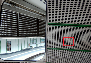
Urban100 ($\times 4$): img_004

HR Bicubic SRCNN FSRCNN VDSR LapSRN MemNet EDSR SRMDNF SCN

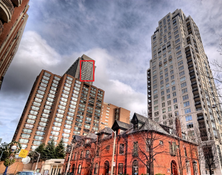
Urban100 ($\times 4$): img_020

HR Bicubic SRCNN FSRCNN VDSR LapSRN MemNet EDSR SRMDNF SCN

Urban100 ($\times 4$): img_095

HR Bicubic SRCNN FSRCNN VDSR LapSRN MemNet EDSR SRMDNF SCN

Figure 4: Visual comparison results of $\times 4$ image super-resolution on Urban100 datasets. SCN achieved qualitative results. More visual comparisons are shown in the supplementary materials.

Figure 5: SCN for JPEG compression artifact removal. From left to right, we show groud truth image, compressed image, and our restored image with scale-wise convolutional network.

4.3 Ablation Study

In this section, we conduct ablation study to justify the significance of proposed scale-wise convolution. The experiments are on image super-resolution with x2 up-scaling.

Multi-scale architectures.

We compare three representative design choices of multi-scale network structures discussed in previous section. The U-Net style model (?) has 2 scales in both encoder and decoder, and 2 residual blocks per scale, then 8 blocks in total. The PSPNet style model (?) has 2 scales and 8 residual blocks per scale, and features from scales are fused in output layer. Our SCN also has 2 scales and 8 residual blocks. The total numbers of parameters of the models are almost the same. Table 6 shows the advances of our proposed SCN over other multi-scale approaches.

Parameter sharing across scales.

We study whether the parameters for different scales can be shared or not. In table 6 we compare (1) single-scale baseline (Baseline), (2) multi-scale architecture without sharing weights (Un-shared), (3) multi-scale architecture with sharing weights (Shared) and (4) a larger model (more parameters) multi-scale architecture without sharing weights. We report their number of parameters in the Table.

Table 6 shows that under same number of parameters, shared version has much better performance. To achieve a similar performance, the un-shared version has to involve more parameters. The results proof the scale-invariance of our proposed SCN and its effectiveness.

Table 4: Ablation study on multi-scale network structures.

Method	PSNR
U-Net style	34.56
PSPNet style	34.58
SCN	34.67

Table 5: Ablation study on parameter sharing across scales.

Method	# Params	PSNR
Baseline	1.2M	34.74
Un-shared	1.2M	34.68
Shared	1.2M	34.77
Un-shared Large	2.1M	34.77

Table 6: Ablation study on re-sampling methods.

Down-sample	Up-sample	PSNR
Conv	Deconv	34.77
AvgPool	Nearest	34.78
Bilinear	Bilinear	34.80

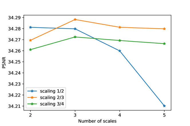
Figure 6: Ablation study on number of scales and scaling ratios.

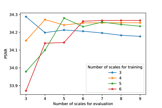
Figure 7: Ablation study on different number of scales for evaluation.

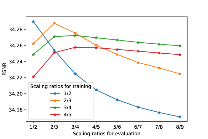
Figure 8: Ablation study on different scaling ratios for evaluation.

Resampling in Scale-wise Convolution.

Scale-wise convolution aggregates information from nearby input scales. A resampling operation is required to fuse features of different scales into the same scale, as shown in Figure 1. In this part, we study the resampling method and compare their performances.

For resampling, there exists several methods: (1) down-sampling with strided convolution, up-sampling with strided deconvolution, (2) down-sampling with average pooling, up-sampling with nearest neighbor sampling and (3) down-sampling with bilinear sampling, up-sampling with bilinear sampling. We note that for the first two methods, the scaling ratio is limited to 2, 4, etc, because the kernel size have to be integer numbers. Our results in Table 6 indicate that biliear has superior performance.

Scales in Scale-wise Convolution.

In this part, we study the number of scales and the scaling ratios between neighborhood scales. From the results in Figure 6, we have several observations. (1) The scaling ratio plays an important role in the performance: a small scaling ratio (e.g., $\frac{1}{2}$) may lead to worse performance as the input feature map being too small, a large scaling ratio (e.g., comparing the curve of $\frac{2}{3}$ and $\frac{3}{4}$) impedes the growth of receptive fields. (2) Multi-scale modeling is essential for image restoration and leads to much better performance compared with single-scale (34.74 in PSNR). Meanwhile more scales may lead to slightly inferior performance, which is likely due to the noise from the smallest scale. For example, in the setting of 6 scales with $\frac{1}{2}$ scaling ratio, the smallest image has resolution $\frac{1}{64}$ of the original resolution.

Evaluation for Scale-wise Convolution.

The convolution on scale axis enables the SCN to be evaluated on number of scales that are different with training. We show in Figure 7 that: (1) When training with limited number of scales, the performance degrades when number of scales between training and evaluation mismatch (e.g., the blue curve for training with 3 scales). (2) When training with enough number of scales, the performance can be boosted even with more scales during evaluation (e.g., the red curve for models trained with 6 scales, the performance grows until 9 scales). We also evaluated models with different scale ratios from training, results in Figure 8 show that scale ratios must be matched between training and evaluation.

5 Conclusions

In this work we have presented scale-wise convolution that models scale-invariance in deep neural networks. The scale-wise convolutional network significantly improves the predictive accuracy on several image restoration datasets including image super-resolution, image denoising and image compression artifact removal. We also conducted experiments to proof the scale-invariance of proposed SCN and show its advances over other multi-scale models.

References

- [Badrinarayanan, Kendall, and Cipolla 2017] Badrinarayanan, V.; Kendall, A.; and Cipolla, R. 2017. Segnet: A deep convolutional encoder-decoder architecture for image segmentation. TPAMI 39(12):2481–2495.
- [Bevilacqua et al. 2012] Bevilacqua, M.; Roumy, A.; Guillemot, C.; and Alberi-Morel, M. L. 2012. Low-complexity single-image super-resolution based on nonnegative neighbor embedding. In BMVC, 135.1–135.10.
- [Cai et al. 2016] Cai, Z.; Fan, Q.; Feris, R. S.; and Vasconcelos, N. 2016. A unified multi-scale deep convolutional neural network for fast object detection. In ECCV, 354–370.
- [Chen and Pock 2016] Chen, Y., and Pock, T. 2016. Trainable nonlinear reaction diffusion: A flexible framework for fast and effective image restoration. TPAMI 39(6):1256–1272.
- [Dabov, Foi, and Egiazarian 2007] Dabov, K.; Foi, A.; and Egiazarian, K. 2007. Video denoising by sparse 3d transform-domain collaborative filtering. In 2007 15th European Signal Processing Conference, 145–149. IEEE.
- [Dong et al. 2014] Dong, C.; Loy, C. C.; He, K.; and Tang, X. 2014. Learning a deep convolutional network for image super-resolution. In ECCV, 184–199.
- [Dong et al. 2015] Dong, C.; Deng, Y.; Change Loy, C.; and Tang, X. 2015. Compression artifacts reduction by a deep convolutional network. In ICCV, 576–584.
- [Dong, Loy, and Tang 2016] Dong, C.; Loy, C. C.; and Tang, X. 2016. Accelerating the super-resolution convolutional neural network. In ECCV, 391–407.
- [Fan et al. 2017] Fan, Y.; Shi, H.; Yu, J.; Liu, D.; Han, W.; Yu, H.; Wang, Z.; Wang, X.; and Huang, T. S. 2017. Balanced two-stage residual networks for image super-resolution. In CVPR Workshops, 1157–1164.
- [Fan et al. 2019] Fan, Y.; Yu, J.; Liu, D.; and Huang, T. S. 2019. An empirical investigation of efficient spatio-temporal modeling in video restoration. In CVPR Workshops.
- [Fan, Yu, and Huang 2018] Fan, Y.; Yu, J.; and Huang, T. S. 2018. Wide-activated deep residual networks based restoration for bpg-compressed images. In CVPR Workshops, 2621–2624.
- [Foi, Katkovnik, and Egiazarian 2007] Foi, A.; Katkovnik, V.; and Egiazarian, K. 2007. Pointwise shape-adaptive dct for high-quality denoising and deblocking of grayscale and color images. TIP 16(5):1395–1411.
- [Fu et al. 2017] Fu, C.-Y.; Liu, W.; Ranga, A.; Tyagi, A.; and Berg, A. C. 2017. Dssd: Deconvolutional single shot detector. arXiv preprint arXiv:1701.06659.
- [Gu et al. 2014] Gu, S.; Zhang, L.; Zuo, W.; and Feng, X. 2014. Weighted nuclear norm minimization with application to image denoising. In CVPR, 2862–2869.
- [Han et al. 2018] Han, W.; Chang, S.; Liu, D.; Yu, M.; Witbrock, M.; and Huang, T. S. 2018. Image super-resolution via dual-state recurrent networks. In CVPR, 1654–1663.
- [Haris, Shakhnarovich, and Ukita 2018] Haris, M.; Shakhnarovich, G.; and Ukita, N. 2018. Deep back-projection networks for super-resolution. In CVPR, 1664–1673.
- [Huang, Singh, and Ahuja 2015] Huang, J.-B.; Singh, A.; and Ahuja, N. 2015. Single image super-resolution from transformed self-exemplars. In CVPR, 5197–5206.
- [Kim, Kwon Lee, and Mu Lee 2016a] Kim, J.; Kwon Lee, J.; and Mu Lee, K. 2016a. Accurate image super-resolution using very deep convolutional networks. In CVPR, 1646–1654.
- [Kim, Kwon Lee, and Mu Lee 2016b] Kim, J.; Kwon Lee, J.; and Mu Lee, K. 2016b. Deeply-recursive convolutional network for image super-resolution. In CVPR, 1637–1645.
- [Lai et al. 2017] Lai, W.-S.; Huang, J.-B.; Ahuja, N.; and Yang, M.-H. 2017. Deep laplacian pyramid networks for fast and accurate super-resolution. In CVPR, 624–632.
- [Li et al. 2018] Li, J.; Fang, F.; Mei, K.; and Zhang, G. 2018. Multi-scale residual network for image super-resolution. In ECCV, 517–532.
- [Lim et al. 2017] Lim, B.; Son, S.; Kim, H.; Nah, S.; and Lee, K. M. 2017. Enhanced deep residual networks for single image super-resolution. In CVPR Workshops, 136–144.
- [Lin et al. 2017] Lin, T.-Y.; Dollár, P.; Girshick, R.; He, K.; Hariharan, B.; and Belongie, S. 2017. Feature pyramid networks for object detection. In CVPR, 2117–2125.
- [Liu et al. 2018] Liu, D.; Wen, B.; Fan, Y.; Loy, C. C.; and Huang, T. S. 2018. Non-local recurrent network for image restoration. In NeurIPS, 1673–1682.
- [Lowe 2004] Lowe, D. G. 2004. Distinctive image features from scale-invariant keypoints. IJCV 60(2):91–110.
- [Martin et al. 2001] Martin, D.; Fowlkes, C.; Tal, D.; and Malik, J. 2001. A database of human segmented natural images and its application to evaluating segmentation algorithms and measuring ecological statistics. In ICCV, volume 2, 416–423.
- [Ronneberger, Fischer, and Brox 2015] Ronneberger, O.; Fischer, P.; and Brox, T. 2015. U-net: Convolutional networks for biomedical image segmentation. In MICCAI, 234–241.
- [Singh and Davis 2018] Singh, B., and Davis, L. S. 2018. An analysis of scale invariance in object detection snip. In CVPR, 3578–3587.
- [Singh, Najibi, and Davis 2018] Singh, B.; Najibi, M.; and Davis, L. S. 2018. Sniper: Efficient multi-scale training. In NeurIPS, 9310–9320.
- [Szegedy et al. 2015] Szegedy, C.; Liu, W.; Jia, Y.; Sermanet, P.; Reed, S.; Anguelov, D.; Erhan, D.; Vanhoucke, V.; and Rabinovich, A. 2015. Going deeper with convolutions. In CVPR, 1–9.
- [Tai et al. 2017] Tai, Y.; Yang, J.; Liu, X.; and Xu, C. 2017. Memnet: A persistent memory network for image restoration. In CVPR, 4539–4547.
- [Tai, Yang, and Liu 2017] Tai, Y.; Yang, J.; and Liu, X. 2017. Image super-resolution via deep recursive residual network. In CVPR, 3147–3155.
- [Timofte et al. 2017] Timofte, R.; Agustsson, E.; Van Gool, L.; Yang, M.-H.; Zhang, L.; Lim, B.; Son, S.; Kim, H.; Nah, S.; Lee, K. M.; et al. 2017. Ntire 2017 challenge on single image super-resolution: Methods and results. In CVPR Workshops, 1110–1121.
- [Timofte, De Smet, and Van Gool 2014] Timofte, R.; De Smet, V.; and Van Gool, L. 2014. A+: Adjusted anchored neighborhood regression for fast super-resolution. In ACCV, 111–126.
- [Xu et al. 2014] Xu, Y.; Xiao, T.; Zhang, J.; Yang, K.; and Zhang, Z. 2014. Scale-invariant convolutional neural networks. arXiv preprint arXiv:1411.6369.
- [Yang et al. 2010] Yang, J.; Wright, J.; Huang, T. S.; and Ma, Y. 2010. Image super-resolution via sparse representation. TIP 19(11):2861–2873.
- [Yu et al. 2016] Yu, J.; Jiang, Y.; Wang, Z.; Cao, Z.; and Huang, T. 2016. Unitbox: An advanced object detection network. In Proceedings of the 24th ACM international conference on Multimedia, 516–520. ACM.
- [Yu et al. 2018] Yu, J.; Fan, Y.; Yang, J.; Xu, N.; Wang, Z.; Wang, X.; and Huang, T. 2018. Wide activation for efficient and accurate image super-resolution. arXiv preprint arXiv:1808.08718.
- [Zeyde, Elad, and Protter 2010] Zeyde, R.; Elad, M.; and Protter, M. 2010. On single image scale-up using sparse-representations. In International conference on curves and surfaces, 711–730.
- [Zhang et al. 2017] Zhang, K.; Zuo, W.; Chen, Y.; Meng, D.; and Zhang, L. 2017. Beyond a Gaussian denoiser: Residual learning of deep CNN for image denoising. TIP 26(7):3142–3155.
- [Zhao et al. 2017] Zhao, H.; Shi, J.; Qi, X.; Wang, X.; and Jia, J. 2017. Pyramid scene parsing network. In CVPR, 2881–2890.