Almost sure Weyl law for quantized tori

Abstract.

We study the eigenvalues of the Toeplitz quantization of complex-valued functions on the torus subject to small random perturbations given by a complex-valued random matrix whose entries are independent copies of a random variable with mean $0$, variance $1$ and bounded fourth moment. We prove that the eigenvalues of the perturbed operator satisfy a Weyl law with probability close to one, which proves in particular a conjecture by T. Christiansen and M. Zworski [4].

1. Introduction

In this paper we consider Toeplitz quantizations of complex-valued functions on the $2d$-dimensional dimensional torus $\mathds{T}^{2d}=\mathds{R}^{2d}/\mathds{Z}^{2d}$. This quantization maps smooth functions to $N^{d}\times N^{d}$ matrices (in general non-selfadjoint),

$$C^{\infty}(\mathds{T}^{2d})\ni p\mapsto p_{N}\in\mathcal{L}(\mathds{C}^{N^{d}},\mathds{C}^{N^{d}}).$$ (1.1)

We will describe this procedure in Section 2 and in detail in Section 3. However, as in [4], we observe that when $d=1$, then $\mathds{T}^{2}=S^{1}_{x}\times S^{1}_{\xi}$ and

$$\begin{split}&f=f(x)\mapsto f_{N}=\mathrm{diag}(f(l/N);l=0,\dots,N-1)\\ &g=g(\xi)\mapsto g_{N}=\mathcal{F}_{N}^{*}\,\mathrm{diag}(g(l/N);l=0,\dots,N-1)\mathcal{F}_{N},\end{split}$$ (1.2)

where $\mathcal{F}_{N}^{*}=N^{-1/2}(\exp(2\pi ik\ell/N))_{0\leq k,\ell\leq N-1}$ is the discrete Fourier transform. In the case of $\mathds{T}^{2}$, the operators $p_{N}$ are also referred to as twisted Toeplitz matrices, see [9, 18].

As an example we may consider the Scottish flag operator [4, 9] given by the symbol

$$p(x,\xi)=\cos(2\pi x)+i\cos(2\pi\xi),\quad(x,\xi)\in\mathds{T}^{2}.$$ (1.3)

From (1.2) we get that

$$p_{N}=\begin{pmatrix}\cos x_{1}&i/2&0&0&\dots&i/2\\ i/2&\cos x_{2}&i/2&0&\dots&0\\ 0&i/2&\cos x_{3}&i/2&\ddots&0\\ \vdots&\ddots&\ddots&\ddots&\ddots&\vdots\\ 0&\dots&0&i/2&\cos x_{N-1}&i/2\\ i/2&0&\dots&0&i/2&\cos x_{N}\\ \end{pmatrix}$$ (1.4)

where $x_{j}=2\pi j/N$, $j=1,\dots,N$.

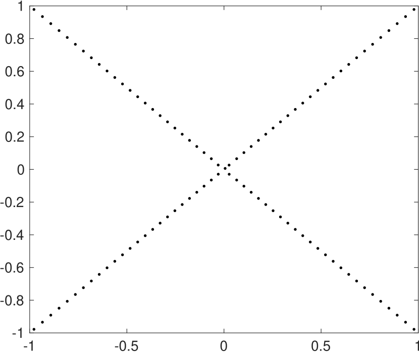
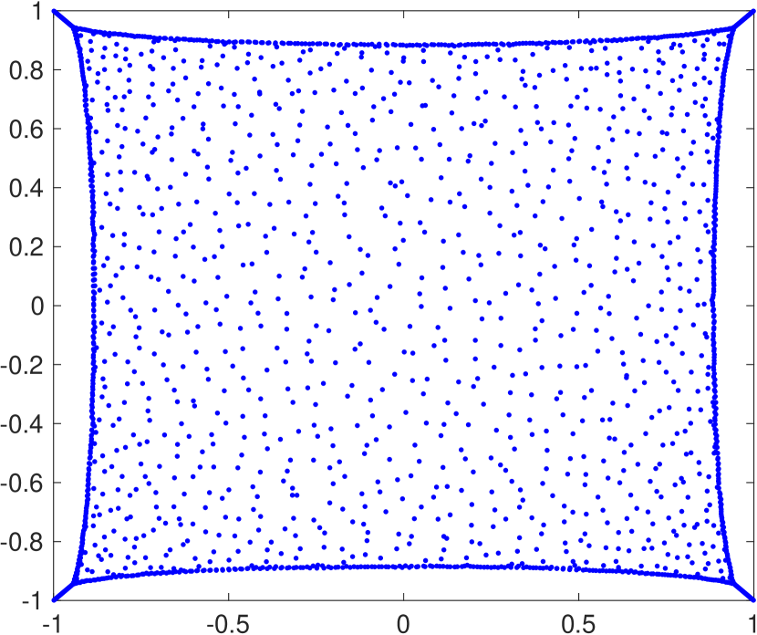
Figure 1. The left hand side shows the spectrum of the unperturbed Scottish flag operator $p_{N}$ (1.3), and the right hand side shows the spectrum of a $p_{N}+\delta Q_{N}$, for $N=1000$, $Q_{N}$ a complex Gaussian random matrix and $\delta=10^{-12}$.

In the recent paper [4] Christiansen and Zworski established a Weyl law for the expected number of eigenvalues of small Gaussian random perturbations of $p_{N}$. They proved

Theorem 1 ([4]).

Suppose that $f\in C^{\infty}(\mathds{T}^{2d})$, and that $\Omega$ is a simply connected open set with a smooth boundary, $\partial\Omega$, such that for all $z$ in a neighbourhood of $\partial\Omega$,

$$\mathrm{vol}_{\mathds{T}^{2d}}(\{w:|f(w)-z|^{2}\leq t\}=\mathcal{O}(t^{\kappa}),\quad 0\leq t\ll 1,$$ (1.5)

with $1/2<\kappa\leq 1$. Let $Q_{N}$ be a complex Gaussian random $N^{d}\times N^{d}$-matrix with independent and identically distributed entries $\sim\mathcal{N}_{\mathds{C}}(0,1)$. Then for any $p\geq p_{0}>d+1/2$

$$\mathds{E}\left(|\mathrm{Spec}(f_{N}+N^{-p}Q_{N})\cap\Omega|\right)=N^{d}\mathrm{vol}_{\mathds{T}^{2d}}(f^{-1}(\Omega))+\mathcal{O}(N^{d-\beta}),$$ (1.6)

for any $\beta<(\kappa-1)(\kappa+1)$.

Let us remark that the original result of [4] is presented with $|f(w)-z|$ in (1.5) instead of $|f(w)-z|^{2}$, which then leads to $1<\kappa\leq 2$. We modified the notation to be more easily comparable with the results that follow.

In Theorem 3 and 8 below we present a stronger result, estimating the probability that this asymptotic holds and providing more precise error estimates. Moreover, we remove the lower bound on $\kappa$ and simply demand it to be $>0$. Furthermore, we allow for a universal probability distribution in the perturbation, see Theorem 8. Finally, we remark that in our results we allow for coupling constants which may go up to the critical case of $N^{-p}$ with $p>d/2$ and down to being sub-exponentially small in $N$.

In [4] the authors state the following

Conjecture 2 ([4]).

Suppose that (1.5) holds for all $z\in\mathds{C}$ with a fixed $0<\kappa\leq 1$. Define random probability measures

$$\mu_{N}=N^{-d}\sum_{\lambda\in\mathrm{Spec}(f_{N}+N^{-p}Q_{N})}\delta_{\lambda},$$

with $p\geq p_{0}>d+1/2$. Then, almost surely

$$\mu_{N}\rightharpoonup f_{*}(\sigma^{n}/n!),\quad N\to\infty,$$

where $\sigma=\sum_{1}^{d}d\xi_{k}\wedge dx_{k}$, $(x,\xi)\in\mathds{T}^{2d}$, is the symplectic form in $\mathds{T}^{2d}$.

We prove this conjecture, see Corollary 9 below, for general random matrix ensembles, and coupling constants $\delta=N^{-p}$, $p>d/2+1$. When $d/2+1\geq p>d/2$ we show that the convergence still holds in probability.

2. Main result

We are interested in the Toeplitz quantization of smooth functions on the $2d$-dimensional torus $\mathds{T}^{2d}=\mathds{R}^{2d}/\mathds{Z}^{d}$. This is related to the more general Berezin-Toeplitz quantization of compact symplectic Kähler manifolds, see [3] or for instance [10] for an introduction. A symbol $p\in C^{\infty}(\mathds{T}^{2d})$ can be identified with a smooth periodic function on $\mathds{R}^{2d}$. Hence $p$ is in the symbol class $S(1)$, i.e. the class of smooth functions $a\in C^{\infty}(\mathds{R}^{2d})$ such that for any $\beta\in\mathds{N}^{2d}$ there exists a constant $C_{\beta}>0$ such that

$$|\partial^{\beta}a(\rho)|\leq C_{\beta}.$$ (2.1)

We let $h\in]0,1]$ denote the semiclassical parameter. A symbol $a\in S(1)$ may depend on $h$, in which case we demand that the constants in the estimates (2.1) are uniform with respect to $h$. The $h$-Weyl quantization of such a symbol $a$ is given by the linear operator

$$a^{w}(x,hD_{x};h)u(x)\stackrel{{\scriptstyle\mathrm{def}}}{{=}}\frac{1}{(2\pi h)^{d}}\iint\mathrm{e}^{\frac{i}{h}\xi(x-y)}a\left(\frac{x+y}{2},\xi;h\right)u(y)dyd\xi,$$

acting on a Schwartz function $u\in\mathcal{S}(\mathds{R}^{d})$. Here, the integral with respect to $\xi$ is to be seen as an oscillatory integral. The operator $a^{w}$ is a continuous linear map $\mathcal{S}\to\mathcal{S}$, $\mathcal{S}^{\prime}\to\mathcal{S}^{\prime}$ and a bounded linear map $L^{2}\to L^{2}$, see for instance in [8, 19, 30].

We denote by $\mathcal{H}_{h}^{d}$ the space of tempered distributions $u\in\mathcal{S}^{\prime}(\mathds{R}^{d})$ which are $\mathds{Z}^{d}$-translation invariant in position and in frequency, more precisely

$$u(x+n)=u(x),\quad\mathcal{F}_{h}(u)(\xi+n)=\mathcal{F}_{h}(u)(\xi),\quad\forall n\in\mathds{Z}^{d}.$$

Here $\mathcal{F}_{h}$ denotes the semiclassical Fourier transform, see (3.10) below for a definition. The space $\mathcal{H}_{h}^{d}$ is $\neq\{0\}$ if and only if $h=1/(2\pi N)$, for some $\mathds{N}\ni N>0$, in which case $\dim\mathcal{H}_{h}^{d}=N^{d}$, and we can identiy $\mathcal{H}_{h}^{d}\simeq\ell^{2}(\mathds{Z}^{d}/N\mathds{Z}^{d})\simeq\mathds{C}^{N^{d}}$.

When $p\in C^{\infty}(\mathds{T}^{2d})$, possibly $h$ dependent in the above sense, then $p^{w}(x,hD_{x})$ maps $\mathcal{H}_{h}^{d}$ into itself, and the restriction

$$p_{N}\stackrel{{\scriptstyle\mathrm{def}}}{{=}}p^{w}(x,hD_{x})\!\upharpoonright_{\mathcal{H}_{h}^{d}}:\mathcal{H}_{h}^{d}\longrightarrow\mathcal{H}_{h}^{d},\quad h=\frac{1}{2\pi N},$$

defines a quantization

$$C^{\infty}(\mathds{T}^{2d})\ni p\mapsto p_{N}\in\mathcal{L}(\mathds{C}^{N^{d}},\mathds{C}^{N^{d}}).$$

The matrix elements of $p_{N}$ (see (3.28) below for details) are given by

$$(p_{N})_{m,j}=\sum_{n,r\in\mathds{Z}^{d}}\widehat{p}(n,j-m-rN)\,\mathrm{e}^{\frac{i\pi}{N}(j+m)\cdot n}(-1)^{n\cdot r},\quad m,j\in(\mathds{Z}/N\mathds{Z})^{d}.$$

where $\widehat{p}$ is the Fourier transform of $p$.

Let $h=1/(2\pi N)$, $\mathds{N}\ni N>0$, and suppose that for $p\in C^{\infty}(\mathds{T}^{2d})$ there exist $p_{\nu}\in C^{\infty}(\mathds{T}^{2d})$, $\nu\in\mathds{N}$, so that

$$p(\rho;h)\sim p_{0}(\rho)+hp_{1}(\rho)+\dots\text{ in }S(1),$$ (2.2)

meaning that $p-\sum_{0}^{M}h^{\nu}p_{\nu}\in h^{M+1}S(1)$ for all $M\in\mathds{N}$. We call $p_{0}$ the principal symbol of $p$.

The aim of this paper is to study the eigenvalue distribution of $p_{N}+\delta Q_{\omega}$ for $\delta$ in a suitable range and for $Q_{\omega}$ in a suitable ensemble of $N^{d}\times N^{d}$ random matrices.

Let $\Omega\Subset\mathds{C}$ be an open relatively compact simply connected set with a uniformly Lipschitz boundary $\partial\Omega$, see Section 7.1.1 below for a precise definition. For $z$ in a neighbourhood of $\partial\Omega$ (denoted by $\text{neigh}(\partial\Omega)$) and $0\leq t\ll 1$ we set

$$V_{z}(t)=\mathrm{Vol}\{\rho\in\mathds{T}^{2d};|p_{0}(\rho)-z|^{2}\leq t\}.$$ (2.3)

We suppose that

$$\exists\kappa\in]0,1],\text{ such that }V_{z}(t)=\mathcal{O}(t^{\kappa}),\text{ uniformly for }z\in\text{neigh}(\partial\Omega),\leavevmode\nobreak\ 0\leq t\ll 1.$$ (2.4)

The first result concerns the case of a perturbation by a complex Gaussian random matrix.

Theorem 3.

Let $p\in C^{\infty}(\mathds{T}^{2d})$ satisfy (2.2) and let $N\geq 2$. Let $\Omega\Subset\mathds{C}$ be an open relatively compact simply connected set with a uniformly Lipschitz boundary $\partial\Omega$, so that (2.4) holds. Let $Q_{\omega}$ be a complex Gaussian random $N^{d}\times N^{d}$-matrix with independent and identically distributed entries, i.e.

$$Q_{\omega}=(q_{i,j}(\omega))_{1\leq i,j\leq N^{d}},\quad q_{i,j}(\omega)\sim\mathcal{N}_{\mathds{C}}(0,1)\leavevmode\nobreak\ (iid).$$ (2.5)

Let $N^{-1}\ll\alpha\ll 1$, let $C>0$ be sufficiently large, and let

$$\varepsilon\gg\alpha^{\kappa}\log\frac{CN^{d/2}}{\delta\alpha^{2}}+\delta N^{\frac{d}{2}}\alpha^{-1/2},\quad 0<\delta\ll N^{-d/2}\alpha^{1/2}.$$ (2.6)

Then,

$$\bigg{|}\#(\mathrm{Spec}(p_{N}+\delta Q_{\omega})\cap\Omega)-{N^{d}}\int_{p_{0}^{-1}(\Omega)}d\rho\bigg{|}\leq\mathcal{O}(N^{d})\left(\int_{p_{0}^{-1}(\partial\Omega+D(0,r))}d\rho+\frac{\varepsilon}{r}+r^{\kappa}\right)$$

for $0<r\ll 1$, with probability

$$\geq 1-\mathcal{O}(r^{-1})\left(N^{d/2}\alpha^{-2}\delta^{-1}\exp\left(\alpha^{-\kappa}(2\delta N^{\frac{d}{2}}\alpha^{-1/2}-\varepsilon/C)\right)+\mathrm{e}^{-N^{d}}\right).$$

This Weyl law shows that the eigenvalues of the small random perturbations of $p_{N}$ roughly equidistribute in $\Sigma=p_{0}(\mathds{T}^{2d})$ the numerical range of the principal symbol of the operator $p_{N}$. This is illustrated in Figure 1. In Corollaries 4, 5, 6, 7, below we provide some special cases of Theorem 3.

A similar result to Theorem 3 for semiclassical pseudo-differential operators on $\mathds{R}^{d}$ has been proven by Hager [13] and Hager-Sjöstrand [14]. Condition (2.4) appears as well in the works of Christiansen-Zworski [4] and Hager-Sjöstrand [14], and is used there, as well as in our work, to control the number of small singular values of $(p_{N}-z)^{*}(p_{N}-z)$ for $z$ in a neighbourhood of $\partial\Omega$.

As observed in [4] for real analytic $p$ condition (2.4) always holds for some $\kappa>0$. Similarly, when $p$ is real analytic and such that $p(\mathds{T}^{2d})\subset\mathds{C}$ has non-empty interior, then

$$\forall z\in\partial\Omega:\leavevmode\nobreak\ dp\!\upharpoonright_{p^{-1}(z)}\neq 0\quad\Longrightarrow\quad\eqref{i2}\text{ holds with }\kappa>1/2.$$ (2.7)

For smooth $p\in C^{\infty}(\mathds{T}^{2d})$ we have that when for every $z\in\partial\Omega$

$$\begin{split}&dp,d\overline{p}\text{ are linearly independent at every point of }p^{-1}(z),\\ &\text{then }\eqref{i2}\text{ holds with }\kappa=1.\end{split}$$ (2.8)

Observe that $dp$ and $d\overline{p}$ are linearly independent at $\rho$ when $\{p,\overline{p}\}(\rho)\neq 0$, where $\{a,b\}=\partial_{\xi}a\cdot\partial_{x}b-\partial_{x}a\cdot\partial_{\xi}b$ denotes the Poisson bracket on $\mathds{T}^{2d}$. Observe that in dimension $d=1$ the condition $\{p,\overline{p}\}\neq 0$ on $p^{-1}(z)$ is equivalent to $dp$, $d\overline{p}$ being linearly independent at every point of $p^{-1}(z)$. However, in dimension $d>1$ this cannot in hold general as the integral of $\{p,\overline{p}\}$ with respect to the Liouville measure on $p^{-1}(z)$ vanishes on every compact connected component of $p^{-1}(z)$, see [20, Lemma 8.1]. Furthermore, condition (2.8) cannot hold when $z\in\partial\Sigma$, $\Sigma=p_{0}(\mathds{T}^{2d})$. However, some iterated Poisson bracket may not be zero there. For example, it was observe in [14, Example 12.1] that

$$\forall\rho\in p^{-1}(\partial\Omega):\leavevmode\nobreak\ \{p,\overline{p}\}(\rho)\neq 0\text{ or }\{p,\{p,\overline{p}\}\}(\rho)\neq 0,\text{ then }\eqref{i2}\text{ holds with }\kappa=\frac{3}{4}.$$ (2.9)

The Poisson bracket has another important role in this context: the link to spectral instability. Indeed

$$\{p,\overline{p}\}(\rho_{0})\neq 0,\leavevmode\nobreak\ \rho_{0}=p(z_{0}),\quad\text{then }\|(p-z_{0})^{-1}\|\geq C_{k}N^{k},\leavevmode\nobreak\ \forall k>0.$$ (2.10)

Moreover, the approximate eigenvector $u_{N}$, with $\|u_{N}\|_{\ell^{2}}=1$, also called a quasimode, causing this resolvent growth at $z_{0}$ can be microlocalized at $\rho_{0}$, i.e. for any smooth function $\chi$ on $\mathds{T}^{2d}$ vanishing near $\rho_{0}$, we have that $\|\chi_{N}u_{N}\|=\mathcal{O}(N^{-\infty})$. This has been shown for $\mathds{T}^{2}$ by Chapman-Trefethen [18], see also [9], and for the Berezin-Toeplitz quantization of compact symplectic Kähler manifolds by Borthwick-Uribe [3]. In these works the condition $\{p,\overline{p}\}(\rho_{0})\neq 0$ is usually referred to as the twist resp. anti-twist condition, depending on the sign of $\{\mathrm{Re\,}p,\mathrm{Im\,}p\}(\rho_{0})$. The construction of such quasimodes goes back to a classical result of Hörmander concerning the local solvability of partial differential equations, see [29] and the references therein. We refer the reader also to [5, 7] for recent results.

In Figure 1 we see that the eigenvalues of the perturbed operator do not fully reach the boundary of $\Sigma$. It is expected that there, under some non-degeneracy condition, such as (2.10), we have improved resolvent bounds on $\|(p_{N}-z_{0})^{-1}\|$, $z_{0}\in\partial\Sigma$. Indeed, Dencker, Sjöstrand and Zworski prove in [7, Theorem 1.4] that under the condition that at least some $k$-fold iterated Poisson bracket of the real and imaginary part of the principal symbol $p_{0}$ does not vanish on $p^{-1}(z_{0})$, $z_{0}\in\partial\Sigma$, the Weyl quantization of the bounded smooth symbol $p\sim p_{0}+hp_{1}+\dots$, satisfies the $L^{2}$ resolvent bound

$$\|(p^{w}-z_{0})^{-1}\|\leq Ch^{-\frac{k}{k+1}}.$$

We suspect (but have not investigated further) that the proof of [7, Theorem 1.4] can be carried over to our situation, with $h=1/2\pi N$, which would then give an explanation of the absence of eigenvalues of $p_{N}+\delta Q_{\omega}$ in Figure 1 in a small $N$-dependent neighbourhood of the boundary $\partial\Sigma$ (away from the edge points of the square $\Sigma$).

Before we turn to the case of more general perturbations, let us discuss some special cases of Theorem 3. Notice that when $\kappa>1/2$ then (2.4) implies that

$$\int_{p_{0}^{-1}(\partial\Omega+D(0,r))}d\rho=\mathcal{O}(r^{2\kappa-1}).$$ (2.11)

One can easily see that $r=\varepsilon^{\frac{1}{2\kappa}}$ minimizes (up to a constant) the error term in Theorem 3, and it becomes

$$\mathcal{O}(N^{d}\varepsilon^{\frac{2\kappa-1}{2\kappa}}).$$

Taking $\alpha=CN^{-1}$ and $\varepsilon=C_{0}N^{-\kappa}(\log N)^{2}$, for some sufficiently large constants $C,C_{0}>1$, one obtains from Theorem 3 the following

Corollary 4.

Under the assumptions of Theorem 3, we let $\kappa\in]1/2,1]$ and set for $p\geq(d+1)/2+\kappa$

$$\delta=\frac{1}{C}N^{-p},$$

for some sufficiently large $C>0$. Then,

$$\bigg{|}\#(\mathrm{Spec}(p_{N}+\delta Q_{\omega})\cap\Omega)-{N^{d}}\int_{p_{0}^{-1}(\Omega)}d\rho\bigg{|}\leq\mathcal{O}\!\left(N^{d-\kappa+1/2}(\log N)^{(2\kappa-1)/\kappa}\right)$$

with probability $\geq 1-\mathcal{O}(N^{-\infty})$.

Notice that at the price of increasing the error term of the eigenvalue counting estimate by a factor $N^{\beta}$, with $\beta\in]0,1[$, one can obtain the above result with probability $\geq 1-\mathrm{e}^{-N^{\beta^{\prime}}/C}$, for some $\beta^{\prime}\in]0,1[$.

For $p_{0}\in]0,\kappa]$, we set $\alpha=CN^{-p_{0}/\kappa}$ and $\varepsilon=C_{0}N^{-p_{0}}(\log N)^{2}$, for some sufficiently large constants $C,C_{0}>1$. Then, one gets from Theorem 3 the following

Corollary 5.

Under the assumptions of Theorem 3, we let $\kappa\in]1/2,1]$ and for $p_{0}\in]0,\kappa]$ set

$$\delta=\frac{1}{C}N^{-(d+1)/2-p_{0}},$$

for some sufficiently large $C>0$. Then,

$$\bigg{|}\#(\mathrm{Spec}(p_{N}+\delta Q_{\omega})\cap\Omega)-{N^{d}}\int_{p_{0}^{-1}(\Omega)}d\rho\bigg{|}\leq\mathcal{O}\!\left(N^{d-p_{0}(2\kappa-1)/(2\kappa)}(\log N)^{(2\kappa-1)/\kappa}\right)$$

with probability $\geq 1-\mathcal{O}(N^{-\infty})$.

Taking $\alpha=CN^{-1}$ and $\varepsilon=C_{0}N^{\beta-\kappa}$, for some sufficiently large constants $C,C_{0}>1$, and $\beta\in]0,\kappa[$, one obtains form Theorem 3 the following

Corollary 6.

Under the assumptions of Theorem 3, we let $\kappa\in]1/2,1]$ and $\beta\in]0,\kappa[$. Set

$$\delta=\mathrm{e}^{-N^{\beta}},$$

then,

$$\bigg{|}\#(\mathrm{Spec}(p_{N}+\delta Q_{\omega})\cap\Omega)-{N^{d}}\int_{p_{0}^{-1}(\Omega)}d\rho\bigg{|}\leq\mathcal{O}\!\left(N^{d+(\beta-\kappa)(2\kappa-1)/(2\kappa)}\right)$$

with probability

$$\geq 1-\mathcal{O}\!\left(\mathrm{e}^{-N^{\beta}/C}\right).$$

When $0<\kappa\leq 1/2$, then, without any additional assumptions on the behaviour of the integral (2.11), we only know that

$$\int_{p_{0}^{-1}(\partial\Omega+D(0,r))}d\rho=o(1),\quad r\to 0,$$

since by the Morse-Sard theorem $p_{0}^{-1}(\partial\Omega)$ has Lebesgue measure $0$, so the regularity of the Lebesgue measure shows the above convergence. In this situation, the best we can have is an error term of order

$$o(N^{d}).$$

Similarly to Corollary 4, 6, we get that

Corollary 7.

Under the assumptions of Theorem 3, we let $\kappa\in]0,1]$ and for $p>d/2$ set

$$\delta=\frac{1}{C}N^{-p},$$

for some sufficiently large $C>0$. Then,

$$\bigg{|}\#(\mathrm{Spec}(p_{N}+\delta Q_{\omega})\cap\Omega)-{N^{d}}\int_{p_{0}^{-1}(\Omega)}d\rho\bigg{|}\leq o(N^{d})$$ (2.12)

with probability $\geq 1-\mathcal{O}(N^{-\infty})$. Moreover, when

$$\delta=\mathrm{e}^{-N^{\beta}},\quad\text{for some }\beta\in]0,\kappa[,$$

then (2.12) holds with probability $\geq 1-\mathcal{O}(\mathrm{e}^{-N^{\beta}/C})$.

The next result concerns the case of a perturbation by an iid matrix.

Theorem 8.

Let $p\in C^{\infty}(\mathds{T}^{2d})$ satisfy (2.2). Let $\Omega\Subset\mathds{C}$ be an open relatively compact simply connected set with a uniformly Lipschitz boundary $\partial\Omega$, so that (2.4) holds. Let $Q_{\omega}$ be a random $N^{d}\times N^{d}$-matrix whose entries are independent copies of a random variable $q$ satisfying

$$\mathds{E}[q]=0,\quad\mathds{E}[|q|^{2}]=1,\quad\mathds{E}[|q|^{4}]<+\infty.$$

For $\delta_{0}>0$ and some sufficiently large $C>0$, let

$$\delta=\frac{1}{C}N^{-d/2-\delta_{0}},$$

and for $\tau\in[0,1[$, set

$$\varepsilon=N^{-\min(\delta_{0},1)\tau\kappa}\log N+N^{-\tau\delta_{0}/2},$$

Then,

$$\bigg{|}\#(\mathrm{Spec}(p_{N}+\delta Q_{\omega})\cap\Omega)-{N^{d}}\int_{p_{0}^{-1}(\Omega)}d\rho\bigg{|}\leq\mathcal{O}(N^{d})\left(\int_{p_{0}^{-1}(\partial\Omega+D(0,r))}d\rho+\frac{\varepsilon}{r}+r^{\kappa}\right),$$

for $0<r\ll 1$, with probability

$$\geq 1-\mathcal{O}(r^{-1})N^{-(1-\tau)\delta_{0}}.$$

Similarly to Corollaries 4, 5, 6, 7, one can use Theorem 8 to get precise error estimates in the various situations.

As a consequence of Theorem 8, or of Theorem 3 in the Gaussian case, we obtain the following result providing a positive response to Conjecture 2 by [4].

Corollary 9.

Let $Q_{\omega}$ and $\delta>0$ be as in Theorem 8 and assume that (2.4) holds uniformly for all $z\in\mathds{C}$. Set

$$\mu_{N}=N^{-d}\sum_{\lambda\in\mathrm{Spec}(p_{N}+{\delta}Q_{\omega})}\delta_{\lambda}.$$

Then, for $\delta_{0}>1$

$$\mu_{N}\rightharpoonup(p_{0})_{*}(d\rho),\quad\text{almost surely},$$

and for $\delta_{0}\in]0,1]$,

$$\mu_{N}\rightharpoonup(p_{0})_{*}(d\rho),\quad\text{in probability.}$$

We remark than in the case of $\mathds{T}^{2d}$ the measure induced by the symplectic volume form $\sigma^{n}/n!$ given in Conjecture 2 is equal to the Lebesgue measure $d\rho$ on $\mathds{T}^{2d}$.

2.1. Related results

The case of Toeplitz matrices given by symbols on $\mathds{T}^{2}$ of the form $\sum_{n\in\mathds{Z}}a_{n}\mathrm{e}^{in\xi}$ was studied in a series of recent works by Davies and Hager [6], Guionnet, Wood and Zeitouni [12], Basak, Paquette and Zeitouni [2, 1], Sjöstrand and the author of the current paper [25, 24]. Such symbols amount to the case of symbols which are constant in the $x$ variable. In these works the non-selfadjointness of the problem does however not come from the symbol itself but from boundary conditions destroying the periodicity of the symbol in $x$ by allowing for a discontinuity. Nevertheless, these works show that by adding some small random noise the limit of the empirical eigenvalues measure $\mu_{N}$ of the perturbed operator converges in probability (or even almost surely in some cases) to $p_{*}(d\rho)$.

In [2] the authors treated in particular the special case of upper triangular banded twisted Toeplitz matrices given by symbols of the form

$$\widetilde{p}(x,\xi)=\sum_{n=0}^{N_{+}}f_{n}(2\pi x)\mathrm{e}^{-2\pi in\xi},\quad(x,\xi)\in\mathds{T}^{2}$$

where $f_{n}$ is only assumed to be a Hölder continuous function and can have a discontinuity. They showed through quite different methods from ours that the $\mu_{N}$ converges weakly in probability to the measure

$$\widetilde{\mu}=\widetilde{p}_{*}(d\rho).$$

Thus we recover this result of [2] (at least in the smooth periodic setting) with Corollary 9. This suggests that the results of Corollary 9 also hold in the case of general twisted Toeplitz matrices with band entries defined by $C^{1}$ functions which are defined on a compact interval with non-periodic boundary conditions.

2.2. Outline of this paper

In Section 3 we recall some fundamental notions and results from standard semiclassical calculus needed in this paper. We use this to describe the procedure to quantize complex-valued function on dilated tori $\mathds{T}^{2d}_{\alpha}$, generalizing the quantization approach presented in [4, 21].

In Section 4 we build on the theory developed in Section 3 and present some functional calculus and estimates on the number of small singular values of Toeplitz quantizations, adapting the approach of [14].

In Section 5 we set up a Grushin problem providing upper bounds on the log determinant of the perturbed operator $\log|\det(p_{N}+\delta Q_{\omega}-z)|$.

In Section 6 we provide probabilistic lower bounds on the number of small singular values of the perturbed operator $(p_{N}+\delta Q_{\omega}-z)$ which yields probabilistic lower bounds on $\log|\det(p_{N}+\delta Q_{\omega}-z)|$. This, together with the estimates of Section 5, can also be seen as a form of concentration inequality for $\log|\det(p_{N}+\delta Q_{\omega}-z)|$.

In Section 7.1 we provide proofs of Theorems 3 and 8 by combining the estimates on $\log|\det(p_{N}+\delta Q_{\omega}-z)|$ with a theorem providing estimates on the number of zeros of holomorphic functions with exponential growth in Lipschitz domains.

In Section 8, we provide a proof of Corollary 9 and in Appendix A we prove a complex version of a result due to Sankar, Spielmann and Teng [22, Lemma 3.2], see also [28, Theorem 2.2].

2.3. Notation

In this paper we frequently use the following notation: when we write $a\ll b$, we mean that $Ca\leq b$ for some sufficiently large constant $C>0$. The notation $f=\mathcal{O}(N)$ means that there exists a constant $C>0$ (independent of $N$) such that $|f|\leq CN$. When we want to emphasize that the constant $C>0$ depends on some parameter $k$, then we write $C_{k}$, or with the above big-O notation $\mathcal{O}_{k}(N)$.

When we write $f=\mathcal{O}(N^{-\infty})$, then we mean that for every $M\in\mathds{N}$, there exists a constant $C_{M}>0$, depending on $M$, such that $|f|\leq C_{M}N^{-M}$. Similarly we will also use the notation $f=\mathcal{O}(h^{\infty})$, with $h\in]0,1]$.

When we write $f=o(1)$, as $N\to\infty$, then we mean that $f\to 0$ as $N\to\infty$. Similarly $f=o(N)$, as $N\to\infty$, means that $N^{-1}f\to 0$ as $N\to\infty$.

Acknowledgments

The author is very grateful to Maciej Zworski for suggesting this project, to László Erdős for some very enlightening discussions and to the Institute of Science and Technology, Austria, where a part of this paper has been written, for providing a welcoming and stimulating environment. The author was supported by a CNRS Momentum grant.

3. Semiclassical calculus

In this section we begin by reviewing some basic notions and properties of semiclassical calculus in $\mathds{R}^{d}$, as can be found for instance in [8, 19, 30]. Afterwards, we will review the Toeplitz quantizaton of functions on the torus, as presented in [4, 21], which roughly speaking consist in restricting the semiclassical calculus to periodic symbols and to function spaces given by tempered distributions which are both periodic in space and in semiclassical frequency.

3.1. Semiclassical quantization

Until further notice we let $h\in]0,1]$ denote the semiclassical parameter. We call $m\in C^{\infty}(\mathds{R}^{2d},]0,\infty[)$ an order function, if there exist $C_{0},N_{0}>0$ such that

$$m(\rho)\leq C_{0}\langle\rho-\mu\rangle^{N_{0}}m(\mu),$$ (3.1)

where $\langle\rho-\mu\rangle=(1+|\rho-\mu|^{2})^{1/2}$. We define the symbol class

$$S(m)\stackrel{{\scriptstyle\mathrm{def}}}{{=}}\{p\in C^{\infty}(\mathds{R}^{2d});\leavevmode\nobreak\ \forall\alpha\in\mathds{N}^{2d}:|\partial^{\alpha}p(\rho)|\leq C_{\alpha}m(\rho)\}.$$ (3.2)

A symbol $p=p(\rho;h)\in S(m)$ may depend on $h\in]0,1]$, in which case we assume that the symbol estimates (3.2) hold uniformly with respect to $h$. If a symbol $p$ is of the form $p(\rho;h)=p_{0}(\rho)+hr(\rho;h)$ with $r\in S(m)$, then we call $p_{0}$ the principal symbol of $p$. We say that $p\in S(m)$ has the asymptotic expansion

$$p\sim p_{0}+hp_{1}+\dots\text{ in }S(m),\quad p_{j}\in S(m),$$ (3.3)

when $p-\sum_{0}^{N}h^{j}p_{j}\in h^{N+1}S(m)$ for any $N\in\mathds{N}$. In fact, given symbols $p_{j}\in S(m)$ we can always find a symbol $p\in S(m)$ by Borel summation, such that (3.3) holds.

The $h$-Weyl quantization of a symbol $p\in S(m)$, acting on a function $u\in\mathcal{S}(\mathds{R}^{d})$ in Schwartz space, is given by

$$p^{w}(x,hD_{x})u(x)=\frac{1}{(2\pi h)^{d}}\iint_{\mathds{R}^{d}}\mathrm{e}^{\frac{i}{h}\xi(x-y)}p\left(\frac{x+y}{2},\xi;h\right)u(y)dyd\xi,$$ (3.4)

where the integral with respect to $\xi$ is to be seen as an oscillatory integral. Integration by parts shows that that the operator $p^{w}(x,hD_{x})$ is continuous $\mathcal{S}(\mathds{R}^{d})\to\mathcal{S}(\mathds{R}^{d})$, and continuous $\mathcal{S}^{\prime}(\mathds{R}^{d})\to\mathcal{S}^{\prime}(\mathds{R}^{d})$ by duality. Moreover, it can be shown that when $m$ is bounded then $p^{w}(x,hD_{x})$ is bounded $L^{2}(\mathds{R}^{d})\to L^{2}(\mathds{R}^{d})$.

Given $a,b\in S(m)$, then

$$a^{w}\circ b^{w}=c^{w},\quad\text{where }c=a\#_{h}b\leavevmode\nobreak\ \in S(m).$$ (3.5)

Here, the product $\#_{h}$ is the bilinear continuous map

$$S(m_{1})\times S(m_{2})\ni(a,b)\mapsto a\#_{h}b\stackrel{{\scriptstyle\mathrm{def}}}{{=}}\mathrm{e}^{\frac{ih}{2}\sigma(D_{x},D_{\xi};D_{y},D_{\eta})}a(x,\xi)b(y,\eta)\big{|}_{y=x,\eta=\xi}\leavevmode\nobreak\ \in S(m_{1}m_{2}),$$ (3.6)

where $\sigma$ denotes the symplectic form on $\mathds{R}^{2d}$, so $\sigma(D_{x},D_{\xi};D_{y},D_{\eta})=D_{\xi}D_{y}-D_{x}D_{\eta}$. We have the following asymptotic expansion

$$a\#_{h}b\sim\sum_{0}^{\infty}\frac{1}{k!}\left(\frac{ih}{2}\sigma(D_{x},D_{\xi};D_{y},D_{\eta})\right)^{k}a(x,\xi)b(y,\eta)\big{|}_{y=x,\eta=\xi}\in S(m_{1}m_{2}).$$ (3.7)

A symbol $a\in S(m)$ is called elliptic if there exists a constant $C>0$, independently of $h>0$, such that

$$|a|\geq\frac{1}{C}m.$$ (3.8)

3.2. Quantization of the torus

We essentially follow the approach of [4, 21] who considered the case $\alpha=1$ of the subsequent. For $\alpha>0$, we define the torus

$$\mathds{T}^{2d}_{\alpha}:=\mathds{R}^{2d}/(\alpha^{-1/2}\mathds{Z})^{2d}.$$ (3.9)

When $\alpha=1$ then we will write $\mathds{T}^{2d}=\mathds{T}^{2d}_{1}$. We define the semiclassical Fourier transform by

$$(\mathcal{F}_{h}u)(\xi)\stackrel{{\scriptstyle\mathrm{def}}}{{=}}\frac{1}{(2\pi h)^{d/2}}\int\mathrm{e}^{\frac{i}{h}\xi x}u(x)dx,\quad u\in\mathcal{S}(\mathds{R}^{d}),$$ (3.10)

which maps $\mathcal{S}\to\mathcal{S}$ continuously and can be extended to a continuous map $\mathcal{S}^{\prime}\to\mathcal{S}^{\prime}$, mapping $L^{2}\to L^{2}$ unitarily.

Let $h\ll\alpha\leq 1$ and set $\widetilde{h}=h/\alpha$. We define the space $\mathcal{H}_{\widetilde{h},\alpha}^{d}\subset\mathcal{S}^{\prime}(\mathds{R}^{d})$ of tempered distributions $u\in\mathcal{S}^{\prime}$ which are both $\alpha^{-1/2}\mathds{Z}^{d}$-periodic in position and in frequency, i.e.

$$u(x+\alpha^{-1/2}n)=u(x),\quad(\mathcal{F}_{\widetilde{h}}u)(\xi+\alpha^{-1/2}n)=(\mathcal{F}_{\widetilde{h}}u)(\xi),\quad\forall n\in\mathds{Z}^{d}.$$ (3.11)

When $\alpha=1$ we will simply write $\mathcal{H}_{h}^{d}=\mathcal{H}_{\widetilde{h},1}^{d}$. The following result was stated in the case $\alpha=1$ in [4, 21].

Lemma 10.

Let $h\ll\alpha\leq 1$. Then, $\mathcal{H}_{\widetilde{h},\alpha}^{d}\neq\{0\}$ if and only if $h=(2\pi N)^{-1}$ for some $N\in\mathds{N}^{*}=\mathds{N}\backslash\{0\}$, in which case $\dim\mathcal{H}_{\widetilde{h},\alpha}^{d}=N^{d}$ and

$$\mathcal{H}_{\widetilde{h},\alpha}^{d}=\mathrm{span}\left\{Q_{k}^{\alpha}=\frac{1}{(\alpha^{1/2}N)^{d/2}}\sum_{n\in\mathds{Z}^{d}}\delta(x-\alpha^{-1/2}(n+k/N));k\in(\mathds{Z}/N\mathds{Z})^{d}\right\}.$$ (3.12)

Proof.

To ease the notation we write $\widehat{u}^{\widetilde{h}}=(2\pi\widetilde{h})^{d/2}\mathcal{F}_{\widetilde{h}}u$, $u\in\mathcal{S}^{\prime}$. Recall the Poisson summation formula (for instance from [15, Section 7.2])

$$\sum_{g\in\mathds{Z}^{d}}\widehat{\psi}^{\widetilde{h}}(g)=\left(\frac{2\pi\widetilde{h}}{a}\right)^{d}\sum_{g\in\mathds{Z}^{d}}\psi\left(\frac{2\pi\widetilde{h}}{a}g\right),\quad\psi\in\mathcal{S},\leavevmode\nobreak\ 0\neq a\in\mathds{R}.$$ (3.13)

Let $\phi\in C^{\infty}_{c}(\mathds{R}^{d};\mathds{R})$ be such that $\sum_{g\in\mathds{Z}^{d}}\phi(x-g)=1$. Suppose that $u\in\mathcal{S}^{\prime}$ is $\alpha^{-1/2}\mathds{Z}^{d}$-periodic in position, as in (3.11). Then for $\psi\in\mathcal{S}$

$$\begin{split}\langle\widehat{u}^{\widetilde{h}},\psi\rangle=\langle u,\widehat{\psi}^{\widetilde{h}}\rangle&=\langle u,\sum_{g}\widehat{\psi}^{\widetilde{h}}(\cdot+g)\phi\rangle\\ &=(2\pi\widetilde{h}\alpha^{1/2})^{d}\langle u,\sum_{g}\psi(2\pi\widetilde{h}\alpha^{1/2}g)\mathrm{e}^{-2\pi i\alpha^{1/2}g\cdot}\phi\rangle,\end{split}$$ (3.14)

where the "$\cdot$" holds the place of the variable in which the distribution acts. In the last equation we applied (3.13) with $a=\alpha^{-1/2}$ to $\psi(y)\mathrm{e}^{-\frac{i}{\widetilde{h}}yx}$, whose $\widetilde{h}$-Fourier transform $y\to\xi$ is given by $\widehat{\psi}^{\widetilde{h}}(\xi+x)$. Hence,

$$\begin{split}&\widehat{u}^{\widetilde{h}}=(2\pi\widetilde{h}\alpha^{1/2})^{d}\sum_{g}c_{g}\delta_{2\pi\widetilde{h}\alpha^{1/2}g},\\ &c_{g}=\langle u,\mathrm{e}^{-2\pi i\alpha^{1/2}g\cdot}\phi\rangle=\langle u,\mathrm{e}^{-2\pi i\alpha^{1/2}g\cdot}\rangle_{\mathds{T}^{d}_{\alpha}},\end{split}$$ (3.15)

where in the last line we see $u\in\mathcal{D}^{\prime}(\mathds{T}^{d}_{\alpha})$ as a distribution on $\mathds{T}^{2d}_{\alpha}$, and $\delta_{x_{0}}=\delta(x-x_{0})$ denotes the Dirac measure at $x_{0}$.

Since $\widehat{u}^{\widetilde{h}}$ is $\alpha^{-1/2}\mathds{Z}^{d}$-translation invariant by (3.11), it follows that

$$\widehat{u}^{\widetilde{h}}=\delta_{\alpha^{-1/2}g}*\widehat{u}^{\widetilde{h}},\quad\forall g\in\mathds{Z}^{d},$$ (3.16)

where $*$ denotes the convolution. Hence, the condition $h=(2\pi N)^{-1}$ for some $N\in\mathds{N}^{*}$ is necessary for $u\neq 0$, as the supports of both sides of (3.16) have to match which is equivalent to the condition $\mathds{Z}^{d}=(2\pi\widetilde{h}\alpha)^{-1}\mathds{Z}^{d}+\mathds{Z}^{d}$.

On the other hand, suppose that $h=(2\pi N)^{-1}$ for some $N\in\mathds{N}^{*}$. The translation invariance (3.11) of $\widehat{u}^{\widetilde{h}}$ implies that $u(x)=\mathrm{e}^{-\frac{i}{\widetilde{h}}\alpha^{-1/2}nx}u(x)$, $n\in\mathds{Z}^{d}$. From (3.15) we then get $c_{g}=c_{g+Nl}$ for all $l\in\mathds{Z}^{d}$. Hence,

$$\begin{split}\widehat{u}^{\widetilde{h}}&=(2\pi\widetilde{h}\alpha^{1/2})^{d}\sum_{j\in(\mathds{Z}/N\mathds{Z})^{d}}c_{j}\sum_{l\in\mathds{Z}^{d}}\delta_{\alpha^{-1/2}(l+N^{-1}j)}\\ &=(2\pi\widetilde{h}\alpha^{1/2})^{d}\sum_{j\in(\mathds{Z}/N\mathds{Z})^{d}}c_{j}\left(\delta_{\alpha^{-1/2}N^{-1}j}*\sum_{l\in\mathds{Z}^{d}}\delta_{l\alpha^{-1/2}}\right)\end{split}$$ (3.17)

Notice that when $0\neq a\in\mathds{R}$ and $u_{a}=\sum_{g\in\mathds{Z}^{d}}\delta_{ag}$, then $\widehat{u}^{\widetilde{h}}_{a}=(2\pi\widetilde{h}/a)^{d}u_{2\pi\widetilde{h}/a}$, see for instance [15, Theorem 7.2.1]. This, together with Fourier inversion formula yields

$$\begin{split}u(x)&=N^{-d}\sum_{j\in(\mathds{Z}/N\mathds{Z})^{d}}c_{j}\sum_{l\in\mathds{Z}^{d}}\exp\left(\frac{i}{\widetilde{h}}N^{-1}\alpha^{-1/2}j\cdot x\right)\delta(x-2\pi\widetilde{h}\alpha^{1/2}l).\\ &=N^{-d}\sum_{j,k\in(\mathds{Z}/N\mathds{Z})^{d}}c_{j}\exp\left(2\pi iN^{-1}j\cdot k\right)\sum_{l^{\prime}\in\mathds{Z}^{d}}\delta(x-\alpha^{-1/2}(l^{\prime}+N^{-1}k)).\end{split}$$ (3.18)

Thus, the condition of the lemma is also sufficient and (3.12) follows as well. ∎

Finally, we remark that the Fourier transform $\mathcal{F}_{\widetilde{h}}$ maps $\mathcal{H}_{\widetilde{h},\alpha}^{d}$ into $\mathcal{H}_{\widetilde{h},\alpha}^{d}$, and can be represented, in the basis (3.12), by

$$(\mathcal{F}_{\widetilde{h}})_{nm}=\frac{\mathrm{e}^{-\frac{2\pi i}{N}n\cdot m}}{N^{d/2}},\quad n,m\in(\mathds{Z}/N\mathds{Z})^{d}.$$ (3.19)

3.3. Quantizing functions on the torus

For $h\ll\alpha\leq 1$ as before, we define an order function on $\mathds{T}^{2d}_{\alpha}$ as follows: let $m\in C^{\infty}(\mathds{T}^{2d}_{\alpha};]0,\infty[)$ be such that there exist constant $C_{0},N_{0}>0$, independently of $\alpha$, such that

$$\begin{split}m(\rho)&\leq C_{0}(1+|\rho-\mu|_{\mathds{T}^{2d}_{\alpha}}^{2})^{N_{0}/2}m(\mu),\\ &\stackrel{{\scriptstyle\mathrm{def}}}{{=}}C_{0}\langle\rho-\mu\rangle_{\mathds{T}^{2d}_{\alpha}}^{N_{0}}m(\mu)\quad\forall\rho,\mu\in\mathds{T}^{2d}_{\alpha},\end{split}$$ (3.20)

where $|\rho-\mu|_{\mathds{T}^{2d}_{\alpha}}:=\inf_{\gamma\in\alpha^{-1/2}\mathds{Z}^{2d}}|\rho-\mu+\gamma|$. When seeing $m$ as a periodic function in $C^{\infty}(\mathds{R}^{2d};]0,\infty[)$, it follows by using the natural projection $\mathds{R}^{2d}\to\mathds{T}^{2d}_{\alpha}$ that $m$ is an order function on $\mathds{R}^{2d}$ in the sense of (3.1).

With this notion of order function we define the symbol class

$$S(m,\alpha)\stackrel{{\scriptstyle\mathrm{def}}}{{=}}\{a\in C^{\infty}(\mathds{T}^{2d}_{\alpha});\leavevmode\nobreak\ \forall\beta\in\mathds{N}^{2d}\leavevmode\nobreak\ \exists\,C_{\beta}>0:\leavevmode\nobreak\ |\partial^{\beta}_{\rho}a(\rho)|\leq C_{\beta}m(\rho)\},$$ (3.21)

where the constant $C_{\beta}>0$ is independent of $\alpha>0$.

Identifying a symbol in $S(m,\alpha)$ with a periodic function in $C^{\infty}(\mathds{R}^{2d})$, we see that $S(m,\alpha)\subset S(m)$. We will use this identification frequently in the sequel whenever convenient. Hence, the quantization procedure discussed in Section 3.1 applies to symbols $p\in S(m,\alpha)$ and it follows immediately from (3.4) by conjugation with the unitary operator $\tau_{\gamma}\mathrm{e}^{ix\cdot\mu/\widetilde{h}}$, $\gamma,\mu\in\alpha^{-1/2}\mathds{Z}^{d}$, where $\tau_{\gamma}u(x)=u(x-\gamma)$, that

$$p^{w}(x,\widetilde{h}D_{x}):\mathcal{H}_{\widetilde{h},\alpha}^{d}\longrightarrow\mathcal{H}_{\widetilde{h},\alpha}^{d},$$ (3.22)

where $\mathcal{H}_{\widetilde{h},\alpha}^{d}\subset\mathcal{S}^{\prime}$.

Therefore, we define for $h=\frac{1}{2\pi N}$, $0<N\in\mathds{N}$, $\widetilde{h}=h/\alpha$

$$p_{N,\alpha}\stackrel{{\scriptstyle\mathrm{def}}}{{=}}p^{w}(x,\widetilde{h}D_{x})\!\upharpoonright_{\mathcal{H}_{\widetilde{h},\alpha}^{d}}\leavevmode\nobreak\ \in\mathcal{L}(\mathcal{H}_{\widetilde{h},\alpha}^{d},\mathcal{H}_{\widetilde{h},\alpha}^{d})$$ (3.23)

When $\alpha=1$ we will simply write $p_{N}=p_{N,1}$. Notice that $1_{N,\alpha}=\mathrm{Id}_{\mathcal{H}_{\widetilde{h},\alpha}^{d}}$.

It follows from (3.6) that $a\#_{\widetilde{h}}b$ is periodic when $a,b\in S(m)$ are periodic. Hence, the composition formula (3.5) applies to symbols $(a,b)\in S(m_{1},\alpha)\times S(m_{2},\alpha)$ and we get

$$a_{N}\circ b_{N}=c_{N},\quad\text{with }c=a\#_{\widetilde{h}}b\in S(m_{1}m_{2},\alpha),\quad h=\frac{1}{2\pi N},\widetilde{h}=\frac{h}{\alpha}.$$ (3.24)

The following result determining the Hilbert space structure of $\mathcal{H}_{\widetilde{h},\alpha}^{d}$ was stated in the case $\alpha=1$ in [4].

Lemma 11.

There exists a unique (up to a multiplicative constant) Hilbert space structure on $\mathcal{H}_{\widetilde{h},\alpha}^{d}$ for which all $f_{N,\alpha}:\mathcal{H}_{\widetilde{h},\alpha}^{d}\to\mathcal{H}_{\widetilde{h},\alpha}^{d}$ with $f\in C^{\infty}(\mathds{T}^{2d}_{\alpha};\mathds{R})$ are self-adjoint. One can choose the constant so that the basis (3.12) is orthonormal. This implies that the Fourier transform on $\mathcal{H}_{\widetilde{h},\alpha}^{d}$ (3.19) is unitary.

Proof.

We can essentially follow the proof of [4, Lemma 2.4], which we present here in an adapted version for the readers convenience. Let $(\bullet|\bullet)_{0}$ denote the scalar product on $\mathcal{H}_{\widetilde{h},\alpha}^{d}$ for which the basis $\{Q_{j}^{\alpha}\}_{j\in(\mathds{Z}/N\mathds{Z})^{d}}$ (3.12) is orthonormal. We write the operator $f^{w}(x,\widetilde{h}D_{x})$ on $\mathcal{H}_{\widetilde{h},\alpha}^{d}$ explicitly in that basis using the Fourier expansion of $f$:

$$\begin{split}&f(x,\xi)=\sum_{n,m\in\mathds{Z}^{d}}\widehat{f}(n,m)\,\mathrm{e}^{2\pi i\alpha^{1/2}(x\cdot n+\xi\cdot m)},\\ &\widehat{f}(n,m)=\alpha^{d}\int_{\mathds{T}^{2d}_{\alpha}}f(x,\xi)\,\mathrm{e}^{-2\pi i\alpha^{1/2}(x\cdot n+\xi\cdot m)}dxd\xi.\end{split}$$ (3.25)

Integration by parts shows that

$$\widehat{f}(n,m)=\mathcal{O}_{k}(1)\langle(n,m)\rangle^{-k}\alpha^{d-k/2}\sum_{|\beta|\leq k}\|\partial^{\beta}f\|_{L^{1}(\mathds{T}^{2d}_{\alpha})}.$$ (3.26)

Write $L_{n,m}(x,\xi)=n\cdot x+m\cdot\xi$, so that

$$f^{w}(x,\widetilde{h}D_{x})=\sum_{n,m\in\mathds{Z}^{d}}\widehat{f}(n,m)\,\mathrm{e}^{2\pi i\alpha^{1/2}L_{n,m}^{w}(x,\widetilde{h}D_{x})}.$$ (3.27)

Since $\mathrm{e}^{2\pi i\alpha^{1/2}L_{n,m}^{w}(x,\widetilde{h}D_{x})}=\mathrm{e}^{i\pi\alpha^{1/2}n\cdot x}\tau_{-2\pi\widetilde{h}\alpha^{1/2}m}\mathrm{e}^{i\pi\alpha^{1/2}n\cdot x}$, we check directly that

$$\mathrm{e}^{2\pi i\alpha^{1/2}L_{n,m}^{w}(x,\widetilde{h}D_{x})}Q^{\alpha}_{j}=\mathrm{e}^{\frac{i\pi}{N}(2n\cdot j-n\cdot m)}Q^{\alpha}_{j-m},$$

where $j-m$ is meant mod $N$. Here $\tau_{a}u(x)=u(x-a)$ is the shift operator. Consequently,

$$\begin{split}&f_{N,\alpha}Q^{\alpha}_{j}=\sum_{m\in(\mathds{Z}/N\mathds{Z})^{d}}F_{m,j}Q_{m}^{\alpha},\\ &F_{m,j}=\sum_{n,r\in\mathds{Z}^{d}}\widehat{f}(n,j-m-rN)\,\mathrm{e}^{\frac{i\pi}{N}(j+m)\cdot n}(-1)^{n\cdot r}.\end{split}$$ (3.28)

Notice that $F_{m,j}$ depends on $\alpha$, although not explicitly denoted here.

Since $\overline{\widehat{f}(n,m)}=\widehat{\overline{f}}(-n,-m)$, we get that

$$\begin{split}\overline{F}_{j,m}&=\sum_{n,r\in\mathds{Z}^{d}}\widehat{\overline{f}}(-n,-(m-j-rN))\,\mathrm{e}^{-\frac{i\pi}{N}(j+m)\cdot n}(-1)^{n\cdot r}\\ &=\sum_{n,r\in\mathds{Z}^{d}}\widehat{\overline{f}}(n,j-m-rN)\,\mathrm{e}^{\frac{i\pi}{N}(j+m)\cdot n}(-1)^{n\cdot r}.\end{split}$$ (3.29)

We see that $\overline{F}_{j,m}=F_{m,j}$ for real-valued $f$. For such an $f$ we see that $f_{N,\alpha}$ is self-adjoint for the inner product $(\bullet|\bullet)_{0}$ and that the map $f\mapsto(F_{m,j})_{j,m\in(\mathds{Z}/N\mathds{Z})^{d}}$ is onto, from $C^{\infty}(\mathds{T}^{2d}_{\alpha})$ to the space of Hermitian matrices.

Any other metric on $\mathcal{H}_{\widetilde{h},\alpha}^{d}$ can be written as $(u|v)=(Bu|v)_{0}=(u|Bv)_{0}$. If $(f_{N,\alpha}u|v)=(u|f_{N,\alpha}v)$ for real-valued $f$, then $B$ and $f_{N,\alpha}$ commute for all such $f$, and hence for all Hermitian matrices. This shows that $B=c\,\mathrm{Id}$, as claimed. ∎

From now on we equip $\mathcal{H}_{\widetilde{h},\alpha}^{d}$ with the inner product $(\bullet|\bullet)_{0}$, for which the basis (3.12) is orthonormal, and drop the subscript. Furthermore, we use this basis to identify

$$\mathcal{H}_{\widetilde{h},\alpha}^{d}\simeq\ell^{2}((\mathds{Z}/N\mathds{Z})^{d})\simeq\mathds{C}^{N^{d}}.$$ (3.30)

Using (3.28), (3.26), we deduce the following result which was presented in the case $\alpha=1$ in [4, Lemma 2.5].

Proposition 12.

Let $f\in S(m,\alpha)$, then

$$\mathrm{tr\,}f_{N,\alpha}=(N\alpha)^{d}\int_{\mathds{T}^{2d}_{\alpha}}f(\rho)d\rho+r_{N},$$

where for every $k\in\mathds{N}$, there exists a constant $C_{k,d}>0$, depending only on $k$ and the dimension $d$, such that

$$|r_{N}|\leq C_{k,d}N^{d-k}\alpha^{d-k/2}\sum_{|\beta|\leq\max(2d+1,k)}\|\partial^{\beta}f\|_{L^{1}(\mathds{T}^{2d}_{\alpha})}.$$

We end this section with a boundedness result.

Proposition 13.

Let $N^{-1}\ll\alpha\leq 1$ and $p\in S(1,\alpha)$. Then, there exists a constant $C>0$, independent of $N$ and $\alpha$, such that

$$\|p_{N,\alpha}\|_{\ell^{2}\to\ell^{2}}\leq C.$$

Proof.

0. In the case when $CN^{-\rho}\leq\alpha\leq 1$ with $\rho\in]0,1[$, we may follow the proof of Proposition 2.7 in [4] with the obvious modifications. We therefore present here only the proof in the critical case $\alpha=N^{-1}C$, $C\gg 1$.

1. We begin by constructing a partition of unity of $\mathds{R}^{2d}$ comprised out of $\alpha^{-1/2}\mathds{Z}^{2d}$ periodic smooth functions. Indeed let $\ell\in[1,2]$ be such that $\alpha^{-1/2}\ell^{-1}=:M\in\mathds{N}$. Let $K=[0,\ell]^{d}$ and let $X\Subset\mathds{R}^{2d}$ be some small open relatively compact $\alpha$-independent neighbourhood of $K$. There exists a $\psi\in C^{\infty}_{c}(X;[0,1])$ such that $\psi\equiv 1$ on $K$ and $\partial_{\rho}^{\eta}\psi(\rho)=\mathcal{O}_{\eta}(1)$, uniformly in $\alpha$, for any $\eta\in\mathds{N}^{2d}$. Set

$$\widetilde{\psi}(\rho)\stackrel{{\scriptstyle\mathrm{def}}}{{=}}\sum_{g\in\mathds{Z}^{2d}}\psi(\rho-\ell g)\geq 1,$$

and notice that $\partial_{\rho}^{\eta}\widetilde{\psi}(\rho)=\mathcal{O}_{\eta}(1)$, uniformly in $\alpha$, for any $\eta\in\mathds{N}^{2d}$. Setting

$$\phi(\rho)\stackrel{{\scriptstyle\mathrm{def}}}{{=}}\frac{\psi(\rho)}{\widetilde{\psi}(\rho)},$$

we see that $\phi\in C^{\infty}_{c}(\mathds{R}^{2d};[0,1])$ with $\mathrm{supp\,}\phi\Subset B(0,C_{0})$, for some constant $C_{0}>0$, independent of $\alpha$, and with $\partial_{\rho}^{\eta}\phi(\rho)=\mathcal{O}_{\eta}(1)$, uniformly in $\alpha$, for any $\eta\in\mathds{N}^{2d}$. Moreover,

$$\sum_{g\in\mathds{Z}^{2d}}\phi(\rho-\ell g)=1,\quad\forall\rho\in\mathds{R}^{2d}.$$ (3.31)

Write $\mathds{Z}^{2d}_{M}=(\mathds{Z}/(M\mathds{Z}))^{2d}$ and set

$$\phi_{\beta}(\rho)\stackrel{{\scriptstyle\mathrm{def}}}{{=}}\sum_{g\in\mathds{Z}^{2d}}\phi\left(\rho-\ell\beta-\alpha^{-1/2}g\right).$$

Notice that $\alpha^{-1/2}=\ell M$. Clearly $\phi_{\beta}\in C^{\infty}(\mathds{R}^{2d};[0,1])$ is a $\alpha^{-1/2}\mathds{Z}^{2d}$-periodic function, such that $\partial_{\rho}^{\eta}\phi_{\beta}(\rho)=\mathcal{O}_{\eta}(1)$, uniformly in $\alpha$, for any $\eta\in\mathds{N}^{2d}$. By (3.31) we get that

$$\sum_{\beta\in\mathds{Z}^{2d}_{M}}\phi_{\beta}(\rho)=1.$$

For $\beta\in\mathds{Z}^{2d}_{M}$ we define

$$p_{\beta}\stackrel{{\scriptstyle\mathrm{def}}}{{=}}\phi_{\beta}\,p.$$

It is well know (see for instance [8, Section 7]) that the composition (3.6) can be written as the oscillatory integral

$$(\overline{p}_{\beta_{1}}\#_{\widetilde{h}}p_{\beta_{2}})(\rho)=\frac{C_{d}}{\widetilde{h}^{2d}}\int_{\mathds{R}^{4d}}\mathrm{e}^{-\frac{i}{\widetilde{h}}\varphi(w)}\overline{p}_{\beta_{1}}(\rho-w_{1})p_{\beta_{2}}(\rho-w_{2})dw$$ (3.32)

where $\varphi(w)=2\sigma(w_{1},w_{2})$ with $|\det\varphi^{\prime\prime}|=2^{4d}$ and with signature $\mathrm{sign}(\varphi^{\prime\prime})=0$.

We split the integral (3.32) into two parts, $I_{1}(\rho)+I_{2}(\rho)$, by using the cut-off functions $\chi(w)$ and $(1-\chi(w))$, where $\chi\in C^{\infty}_{c}(\mathds{R}^{4d};[0,1])$ is equal to $1$ on $B(0,1)$ and equal to $0$ on $\mathds{R}^{4d}\backslash B(0,2)$.

2. For $\gamma\in\mathds{N}^{2d}$ we take the $\partial^{\gamma}_{\rho}$ derivative of $I_{1}$ and obtain

$$\partial^{\gamma}_{\rho}I_{1}(\rho)=\frac{C_{d}}{\widetilde{h}^{2d}}\int_{\mathds{R}^{4d}}\mathrm{e}^{-\frac{i}{\widetilde{h}}\phi(w)}\chi(w)\partial^{\gamma}_{\rho}(\overline{p}_{\beta_{1}}(\rho-w_{1})p_{\beta_{2}}(\rho-w_{2}))dw.$$

The method of stationary phase, see for instance [8, Proposition 5.2], yields that

$$\begin{split}&\partial^{\gamma}_{\rho}I_{1}(\rho)\\ &=\mathcal{O}_{d}(1)\left(\partial^{\gamma}_{\rho}(\overline{p}_{\beta_{1}}(\rho)p_{\beta_{2}}(\rho))+\widetilde{h}\sum_{|\eta|\leq 4d+3}\sup_{|w|\leq 2}\left|\partial^{\eta}_{w}\chi(w)\partial^{\gamma}_{\rho}(\overline{p}_{\beta_{1}}(\rho-w_{1})p_{\beta_{2}}(\rho-w_{2}))\right|\right).\end{split}$$ (3.33)

Notice that the terms on the right hand side are equal to $0$ unless $|w|\leq 2$ and

$$\begin{split}&|\rho-w_{1}-\ell\beta_{1}|_{\mathds{T}^{2d}_{\alpha}}=\inf\limits_{g\in\mathds{Z}^{2d}}|\rho-w_{1}-\ell\beta_{1}-\alpha^{-1/2}g|\leq C_{0},\\ &|\rho-w_{2}-\ell\beta_{2}|_{\mathds{T}^{2d}_{\alpha}}\leq C_{0}.\end{split}$$ (3.34)

Then,

$$\begin{split}|\ell\beta_{1}-\ell\beta_{2}|_{\mathds{T}^{2d}_{\alpha}}&\leq|\rho-w_{1}-\ell\beta_{1}|_{\mathds{T}^{2d}_{\alpha}}+|\rho-w_{2}-\ell\beta_{2}|_{\mathds{T}^{2d}_{\alpha}}+|w_{1}|_{\mathds{T}^{2d}_{\alpha}}+|w_{2}|_{\mathds{T}^{2d}_{\alpha}}\\ &\leq 2C_{0}+4,\end{split}$$ (3.35)

and similarly

$$\begin{split}\left|\rho-\frac{\ell\beta_{1}+\ell\beta_{2}}{2}\right|_{\mathds{T}^{2d}_{\alpha}}&\leq\frac{1}{2}|\rho-w_{1}-\ell\beta_{1}|_{\mathds{T}^{2d}_{\alpha}}+\frac{1}{2}|\rho-w_{2}-\ell\beta_{2}|_{\mathds{T}^{2d}_{\alpha}}+\frac{1}{2}|w_{1}|_{\mathds{T}^{2d}_{\alpha}}+\frac{1}{2}|w_{2}|_{\mathds{T}^{2d}_{\alpha}}\\ &\leq C_{0}+2.\end{split}$$ (3.36)

Since all derivatives of $p\in S(1,\alpha)$ are bounded, we deduce from (3.33), (3.35), (3.36) that for any $K\in\mathds{N}$, $\gamma\in\mathds{N}^{2d}$, $\beta_{1},\beta_{2}\in\mathds{Z}^{2d}_{M}$

$$|\partial^{\gamma}_{\rho}I_{1}(\rho)|\leq\mathcal{O}_{d,\gamma,K}(1)\langle\ell\beta_{1}-\ell\beta_{2}\rangle_{\mathds{T}^{2d}_{\alpha}}^{-K}\left\langle\rho-\frac{\ell\beta_{1}+\ell\beta_{2}}{2}\right\rangle_{\mathds{T}^{2d}_{\alpha}}^{-K}.$$ (3.37)

3. Next, we turn to the second part of (3.32)

$$I_{2}(\rho)=\frac{C_{d}}{\widetilde{h}^{2d}}\int_{\mathds{R}^{4d}}\mathrm{e}^{-\frac{i}{\widetilde{h}}\varphi(w)}(1-\chi(w))\overline{p}_{\beta_{1}}(\rho-w_{1})p_{\beta_{2}}(\rho-w_{2})dw.$$

Since the integrand is equal to $0$ when $|w|\leq 1$, and $|\nabla\varphi|=2|w|$, we set ${}^{t}L=|\nabla\varphi|^{-2}\nabla\varphi\cdot\frac{\widetilde{h}}{i}\nabla$, and obtain from integration by parts that for any $\gamma\in\mathds{N}^{2d}$ and $T\in\mathds{N}$ sufficiently large,

$$\begin{split}|\partial_{\rho}^{\gamma}I_{2}(\rho)|&=\left|\frac{C_{d}}{\widetilde{h}^{2d}}\int_{\mathds{R}^{4d}}\mathrm{e}^{-\frac{i}{\widetilde{h}}\varphi(w)}L^{T}\big{(}(1-\chi(w))\partial_{\rho}^{\gamma}(\overline{p}_{\beta_{1}}(\rho-w_{1})p_{\beta_{2}}(\rho-w_{2}))\big{)}dw\right|\\ &\leq\mathcal{O}_{d,\gamma,T}(1)\widetilde{h}^{T-2d}\int_{|w|\geq 1}\frac{f_{\beta_{1}}(\rho-w_{1})f_{\beta_{2}}(\rho-w_{2})}{|w|^{T}}dw,\end{split}$$ (3.38)

where $f_{\beta_{i}}(\rho-w_{i}-\beta_{i})$, $i=1,2$, are bounded continuous functions which are equal to $0$ unless (3.34) holds. Since $|w|\geq 1$, we obtain similarly to (3.35), (3.36) that

$$\begin{split}|\ell\beta_{1}-\ell\beta_{2}|_{\mathds{T}^{2d}_{\alpha}}&\leq 2C_{0}+\sqrt{2}|w|_{\mathds{T}^{2d}_{\alpha}}\\ &\leq\mathcal{O}(1)|w|,\end{split}$$ (3.39)

and

$$\begin{split}\left|\rho-\frac{\ell\beta_{1}+\ell\beta_{2}}{2}\right|_{\mathds{T}^{2d}_{\alpha}}&\leq C_{0}+\frac{\sqrt{2}}{2}|w|_{\mathds{T}^{2d}_{\alpha}}\\ &\leq\mathcal{O}(1)|w|.\end{split}$$ (3.40)

Here we used that $|w|_{\mathds{T}^{2d}_{\alpha}}\leq|w|$. Hence, taking $T\in\mathds{N}$ in (3.38) sufficiently large, we obtain that for any $K\in\mathds{N}$, $\gamma\in\mathds{N}^{2d}$, $\beta_{1},\beta_{2}\in\mathds{Z}^{2d}_{M}$,

$$|\partial_{\rho}^{\gamma}I_{2}(\rho)|\leq\mathcal{O}_{d,\gamma,K}(1)\langle\ell\beta_{1}-\ell\beta_{2}\rangle_{\mathds{T}^{2d}_{\alpha}}^{-K}\left\langle\rho-\frac{\ell\beta_{1}+\ell\beta_{2}}{2}\right\rangle_{\mathds{T}^{2d}_{\alpha}}^{-K}.$$ (3.41)

4. Recall the definition (3.20) and notice that for any $\beta_{1},\beta_{2}\in\mathds{Z}^{2d}_{M}$, $K\in\mathds{N}\backslash\{0\}$

$$m_{\beta_{1},\beta_{2}}(\rho)\stackrel{{\scriptstyle\mathrm{def}}}{{=}}\langle\ell\beta_{1}-\ell\beta_{2}\rangle_{\mathds{T}^{2d}_{\alpha}}^{-K}\left\langle\rho-\frac{\ell\beta_{1}+\ell\beta_{2}}{2}\right\rangle_{\mathds{T}^{2d}_{\alpha}}^{-K}.$$ (3.42)

is an order function on $\mathds{T}^{2d}_{\alpha}$. Since the constants in the estimates (3.37) and (3.41) are independent of $N$ and $\alpha$, it follows that $\overline{p}_{\beta_{1}}\#_{\widetilde{h}}p_{\beta_{2}}\in S(m_{\beta_{1},\beta_{2}},\alpha)$. By (3.24), we then see that

$$q_{\beta_{1},\beta_{2}}\stackrel{{\scriptstyle\mathrm{def}}}{{=}}p_{\beta_{1}}\#_{\widetilde{h}}\overline{p}_{\beta_{2}}\#_{\widetilde{h}}\overline{p}_{\beta_{1}}\#_{\widetilde{h}}p_{\beta_{2}}\in S(m_{\beta_{1},\beta_{2}}^{2},\alpha).$$ (3.43)

Using the calculus (3.24) and Proposition (12), we get that

$$\begin{split}\|(p_{\beta_{1}})^{*}_{N}&(p_{\beta_{2}})_{N}\|_{\mathrm{HS}}^{2}\\ &=\mathrm{tr\,}(p_{\beta_{2}})^{*}_{N}(p_{\beta_{1}})_{N}(p_{\beta_{1}})^{*}_{N}(p_{\beta_{2}})_{N}\\ &=(N\alpha)^{d}\left(\int_{\mathds{T}^{2d}_{\alpha}}q_{\beta_{1},\beta_{2}}(\rho)d\rho+\mathcal{O}(N\alpha^{1/2})^{-1}\sum_{|\gamma|\leq 2d+1}\|\partial^{\gamma}q_{\beta_{1},\beta_{2}}\|_{L^{1}(\mathds{T}^{2d}_{\alpha})}\right).\end{split}$$ (3.44)

Taking $K\in\mathds{N}$ in (3.42) sufficiently large, we can estimate the first integral by

$$\begin{split}\left|\int_{\mathds{T}^{2d}_{\alpha}}q_{\beta_{1},\beta_{2}}(\rho)d\rho\right|&\leq\mathcal{O}(1)\int_{\mathds{T}^{2d}_{\alpha}}m_{\beta_{1},\beta_{2}}(\rho)d\rho\\ &\leq\mathcal{O}(1)\langle\ell\beta_{1}-\ell\beta_{2}\rangle_{\mathds{T}^{2d}_{\alpha}}^{-K}\int_{\mathds{R}^{2d}}\left\langle\rho\right\rangle^{-K}d\rho\\ &=\mathcal{O}(1)\langle\ell\beta_{1}-\ell\beta_{2}\rangle_{\mathds{T}^{2d}_{\alpha}}^{-K}.\end{split}$$ (3.45)

Here, to see the second inequality, we split $\mathds{T}^{2d}_{\alpha}\simeq[0,\alpha^{-1/2}]^{d}$ into $2^{d}$ translates of the cube $[0,\alpha^{-1/2}/2]^{d}$ and used the translation invariance of the Lebesgue measure.

Similarly, we have that

$$\|\partial^{\gamma}q_{\beta_{1},\beta_{2}}\|_{L^{1}(\mathds{T}^{2d}_{\alpha})}=\mathcal{O}(1)\langle\ell\beta_{1}-\ell\beta_{2}\rangle_{\mathds{T}^{2d}_{\alpha}}^{-K}.$$ (3.46)

Using that $\alpha=CN^{-1}$, $C\gg 1$, we get from (3.44), (3.45), (3.46), that

$$\|(p_{\beta_{1}})^{*}_{N}(p_{\beta_{2}})_{N}\|_{\ell^{2}\to\ell^{2}}\leq\mathcal{O}(1)\langle\ell\beta_{1}-\ell\beta_{2}\rangle_{\mathds{T}^{2d}_{\alpha}}^{-K}.$$ (3.47)

Using that $\alpha^{-1/2}=\ell M$, we get that for $K\in\mathds{N}$ sufficiently large, there exists a constant $C>0$, independent of $N$, such that

$$\sup\limits_{\beta_{1}\in\mathds{Z}^{2d}_{M}}\sum_{\beta_{2}\in\mathds{Z}^{2d}_{M}}\|(p_{\beta_{1}})^{*}_{N}(p_{\beta_{2}})_{N}\|_{\ell^{2}\to\ell^{2}}\leq C,$$ (3.48)

and similarly

$$\sup\limits_{\beta_{1}\in\mathds{Z}^{2d}_{M}}\sum_{\beta_{2}\in\mathds{Z}^{2d}_{M}}\|(p_{\beta_{1}})_{N}(p_{\beta_{2}})^{*}_{N}\|_{\ell^{2}\to\ell^{2}}\leq C.$$ (3.49)

Hence, by the Cotlar-Stein Lemma, see for instance [8, Lemma 7.2], $p_{N}=\sum_{\beta\in\mathds{Z}^{2d}_{M}}(p_{\beta})_{N}$ converges strongly and $\|p_{N}\|_{\ell^{2}\to\ell^{2}}\leq C$. ∎

4. Functional calculus

We begin by recalling the functional calculus for pseudo-differential operators, as presented in [8, Section 8], adapted to symbols in the class $S(m,\alpha)$ (3.21). The following Proposition 14 in the case when $N^{-\rho}C\leq\alpha\ll 1$, $\rho\in]0,1[$, has been proven in [4, Lemma 2.8]. The following result gives and extension including the critical case when $\alpha=CN^{-1}$, $C\gg 1$.

Proposition 14.

Let $N^{-1}\ll\alpha\ll 1$. Let $m\geq 1$ be an order function satisfying (3.20), and let $p^{w}(x,\widetilde{h}D_{x};h,\alpha)$ be a selfadjoint operator with $0\leq p\in S(m,\alpha)$, and $p\sim\sum_{0}^{\infty}\widetilde{h}^{\nu}p_{\nu}$ in $S(m,\alpha)$, and with $p+i$ elliptic. Then, for every $\psi\in C^{\infty}_{c}(\mathds{R})$

$$\psi(p_{N,\alpha})=f_{N,\alpha},\quad f\in S(1/m,\alpha)$$ (4.1)

and

$$f\sim\sum_{0}^{\infty}\widetilde{h}^{\nu}f_{\nu}(\rho;\alpha)\text{ in }S(1/m,\alpha),\quad f_{\nu}\in S(1/m,\alpha).$$ (4.2)

In particular, $f_{0}(\rho;\alpha)=\psi(p_{0}(\rho))$ and

$$f_{\nu}(\rho;\alpha)=\sum_{j=1}^{2\nu}g_{j}(\rho,\alpha)\psi^{(j)}(p_{0}(\rho)),\quad g_{j}\in S(1,\alpha).$$ (4.3)

Remark 15.

We recall that in the above Proposition, although not denoted explicitly, $p,p_{\nu}\in S(m,\alpha)$ may depend on $\alpha$, however with the constants in the symbol estimates (3.21) being independent of $\alpha$.

Proof of Proposition 14.

We employ the approach to the functional calculus of pseudo-differential operators via the Helffer-Sjöstrand formula: For self-adjoint operators $A$, it follows from the spectral theorem and the fact that $(\pi z)^{-1}$ is a fundamental solution to $\partial_{\bar{z}}$ on $\mathds{C}$, that

$$\psi(A)=-\frac{1}{\pi}\int(z-A)^{-1}\partial_{\bar{z}}\widetilde{\psi}(z)L(dz).$$ (4.4)

Here $L(dz)$ denotes the Lebesgue measure on $\mathds{C}$ and $\widetilde{\psi}\in C_{c}^{\infty}(\mathds{C})$ is an almost holomorphic extension of $\psi$, satisfying $\widetilde{\psi}\!\upharpoonright_{\mathds{R}}=\psi$ and $\partial_{\bar{z}}\widetilde{\psi}(z)=\mathcal{O}(|\mathrm{Im\,}z|^{\infty})$, see [8, Chapter 8] for more details.

Since $p+i$ is elliptic, so is $p-z$ for $|z|\leq C$ and $\mathrm{Im\,}z\neq 0$. By Beals’ Lemma, see for instance [8, Proposition 8.3], it follows that $(z-p^{w})^{-1}=r^{w}$ with $r\in S(1)$. In fact $r\in S(1,\alpha)$. To see this notice first that conjugating $a^{w}(x,\widetilde{h}D_{x})$, $a\in S(m^{\prime})$ for some order function $m^{\prime}$, with the unitary operator $\exp(iL(x,\widetilde{h}D_{x})/\widetilde{h})$, $L(x,\widetilde{h}D_{x})=x^{*}\cdot x+\xi^{*}\cdot\widetilde{h}D_{x}$, $\xi^{*},x^{*}\in\mathds{R}^{d}$, we get

$$\mathrm{e}^{\frac{i}{\widetilde{h}}L(x,\widetilde{h}D_{x})}a^{w}(x,\widetilde{h}D_{x})\mathrm{e}^{-\frac{i}{\widetilde{h}}L(x,\widetilde{h}D_{x})}=(a\circ\phi_{1})^{w}(x,\widetilde{h}D_{x}).$$

Here $\phi_{t}$ is the flow at time $t$ associated with the Hamilton vector field $H_{L}=(\xi^{*},-x^{*})$ generated by $L$. In particular $a\circ\phi_{1}(x,\xi)=a(x+\xi^{*},\xi-x^{*})\in S(m^{\prime})$. Setting $x^{*}=\alpha^{-1/2}m$, $\xi^{*}=-\alpha^{-1/2}n$, for $n,m\in\mathds{Z}^{d}$, and using the $\alpha^{-1/2}\mathds{Z}^{2d}$-translation invariance of $p$, we get

$$(r\circ\phi_{1})^{w}=\mathrm{e}^{\frac{i}{\widetilde{h}}L}r^{w}\mathrm{e}^{-\frac{i}{\widetilde{h}}L}=(z-\mathrm{e}^{\frac{i}{\widetilde{h}}L}p^{w}\mathrm{e}^{-\frac{i}{\widetilde{h}}L})^{-1}=(z-p^{w})^{-1}=r^{w}.$$

This equality holds in the space of linear continuous maps $\mathcal{S}\to\mathcal{S}^{\prime}$, so by the Schwartz’ kernel theorem $r\circ\phi_{1}=r$ in $\mathcal{S}^{\prime}$, and therefore $r\circ\phi_{1}=r$ point-wise since both are smooth functions. Since $n,m$ where chosen arbitrarily, it follows that $r\in C^{\infty}(\mathds{T}^{2d}_{\alpha})$, and in particular that $r\in S(1,\alpha)$.

Next, applying the modified Beals’ symbol estimates as in [8, Proposition 8.6] and proceeding as in the proof of Proposition 8.7 and of (8.19) [8], it follows that $\psi(p^{w})=f^{w}$ with $f\in S(1/m,\alpha)$, satisfying (4.2), (4.3).

The above discussion shows that $r_{N}=(z-p_{N})^{-1}$, so by (4.4), we see that

$$\psi(p_{N,\alpha})=\psi(p^{w}\!\upharpoonright_{\mathcal{H}_{\widetilde{h},\alpha}^{d}})=\psi(p^{w})\!\upharpoonright_{\mathcal{H}_{\widetilde{h},\alpha}^{d}}$$

and (4.1) follows. ∎

4.1. Phase space dilation

Until further notice we let $h=1/(2\pi N)$, $0<N\in\mathds{N}$ and $h\ll\alpha\ll 1$. Let $p\in C^{\infty}(\mathds{T}^{2d})$ with $p\sim p_{0}+hp_{1}+\dots$ in $S(1,1)$. Then, $P=p^{w}(x,hD_{x};h)$ is a bounded operator $L^{2}(\mathds{R}^{d})\to L^{2}(\mathds{R}^{d})$. Setting $Q=P^{*}P$, we see, by the semiclassical calculus reviewed in Section 3, that the selfadjoint operator

$$\begin{split}&Q=q^{w}(x,hD_{x};h)\text{ has the symbol }\\ &q=\overline{p}\#_{h}p\sim q_{0}+hq_{1}+\dots\text{ in }S(1,1),\quad\text{with }q_{0}=|p_{0}|^{2}.\end{split}$$ (4.5)

The transformation

$$(U_{\alpha}\phi)(x)=\alpha^{d/4}\phi(\alpha^{1/2}x),\quad\phi\in\mathcal{S}(\mathds{R}^{d}),$$ (4.6)

is a continuous bijection $\mathcal{S}\to\mathcal{S}$, and $\mathcal{S}^{\prime}\to\mathcal{S}^{\prime}$ by duality. Notice that the factor $\alpha^{d/4}$ has been chosen so that $U_{\alpha}:L^{2}\to L^{2}$ unitarily with $U_{\alpha}^{*}=U_{\alpha}^{-1}=U_{\alpha^{-1}}$. Moreover, $U_{\alpha}$ maps $C^{\infty}(\mathds{T}^{2d})\to C^{\infty}(\mathds{T}^{2d}_{\alpha})$ continuously, and $\mathcal{H}_{h,1}^{d}\to\mathcal{H}_{\widetilde{h},\alpha}^{d}$ unitarily with respect to the inner products introduced in Lemma 11. In particular, we see by (3.12) that

$$U_{\alpha}Q_{j}^{1}=Q_{j}^{\alpha}.$$ (4.7)

Using $U_{\alpha}$ we perform the phase space dilation $\mathds{T}^{2d}\ni(x,\xi)=\alpha^{1/2}(\widetilde{x},\widetilde{\xi})$, $(\widetilde{x},\widetilde{\xi})\in\mathds{T}^{2d}_{\alpha}$, and get

$$q^{w}(x,hD_{x};h)=U_{\alpha}^{-1}q^{w}(\alpha^{1/2}(\widetilde{x},\widetilde{h}D_{\widetilde{x}});h)U_{\alpha},\quad\widetilde{h}=\frac{h}{\alpha}.$$ (4.8)

Writing $\widetilde{q}(\widetilde{\rho};h):=q(\alpha^{1/2}\widetilde{\rho};h)\in S(1,\alpha)$, we conclude from the mapping properties discussed after (4.6), that

$$q_{N}=q^{w}(x,hD_{x};h)\!\upharpoonright_{\mathcal{H}_{h,1}^{d}}=U_{\alpha}^{-1}\left(\widetilde{q}^{w}(\alpha^{1/2}(\widetilde{x},\widetilde{h}D_{\widetilde{x}});h)\!\upharpoonright_{\mathcal{H}_{\widetilde{h},\alpha}^{d}}\right)U_{\alpha}=U_{\alpha}^{-1}\widetilde{q}_{N,\alpha}U_{\alpha}.$$ (4.9)

Next, we follow the ideas of [14, Section 4], and pass to a new order function adapted to the rescaled symbol $\alpha^{-1}\widetilde{q}$. Furthermore, we drop the tilde on the variable $\rho$ to ease the notation. Since $q_{0}\in S(1,1)$, we see that

$$m(\rho)\stackrel{{\scriptstyle\mathrm{def}}}{{=}}1+\frac{q_{0}(\alpha^{1/2}\rho)}{\alpha}\geq 1,\quad\rho\in\mathds{T}^{2d}_{\alpha},$$ (4.10)

is a function in $C^{\infty}(\mathds{T}^{2d}_{\alpha})$. We check that it satisfies the estimate for an order function (3.20). Indeed, for $|\beta|=1$

$$\partial_{\rho}^{\beta}m(\rho)=\frac{(\partial_{\rho}^{\beta}q_{0})(\alpha^{1/2}\rho)}{\alpha^{1/2}}\leq C\frac{q_{0}^{1/2}(\alpha^{1/2}\rho)}{\alpha^{1/2}}\leq C\,m(\rho)^{1/2},$$

and for $|\beta|=2$

$$\partial_{\rho}^{\beta}m(\rho)=(\partial_{\rho}^{\beta}q_{0})(\alpha^{1/2}\rho)\leq C,$$

where the constant $C>0$ (not necessarily the same in both inequalities) is independent of $\alpha$. Hence, we get by Taylor expansion that for $\rho,\mu\in\mathds{R}^{2d}$

$$m(\rho)\leq m(\mu)+Cm(\rho)^{1/2}|\rho-\mu|+C|\rho-\mu|^{2},$$

and since $m\geq 1$ that

$$m(\rho)\leq C\langle\rho-\mu\rangle^{2}m(\mu).$$

Using the $\alpha^{-1/2}\mathds{Z}^{2d}$-translation invariance of $m$, we see that for any $\rho^{\prime},\mu^{\prime}\in\mathds{T}^{2d}_{\alpha}$ and any $\gamma\in\mathds{Z}^{2d}$

$$m(\rho^{\prime})\leq C\langle\rho^{\prime}-\mu^{\prime}+\alpha^{-1/2}\gamma\rangle^{2}m(\mu).$$

Since this holds for any $\gamma$ it also holds for the infimum over $\gamma\in\mathds{Z}^{2d}$, and we deduce that $m$ satisfies (3.20).

Similarly, we get the following symbol estimates (with respect to the new order function $m$ (4.10))

$$\begin{split}&\widetilde{q}(\rho)\leq m(\rho)\\ &\partial^{\beta}_{\rho}\widetilde{q}(\rho)=\mathcal{O}(1)m(\rho)^{1/2},\quad|\beta|=1\\ &\partial^{\beta}_{\rho}\widetilde{q}(\rho)=\mathcal{O}(1),\quad|\beta|=2\\ &\partial^{\beta}_{\rho}\widetilde{q}(\rho)=\mathcal{O}(1)\alpha^{|\beta|/2-1},\quad|\beta|\geq 2.\end{split}$$ (4.11)

and in general

$$\partial^{\beta}_{\rho}\widetilde{q}(\rho)=\mathcal{O}_{\beta}(1)m(\rho).$$ (4.12)

We note that in the above equations the constants $\mathcal{O}(1)$ are independent of $\alpha$. Hence, $\widetilde{q}\in S(m,\alpha)$, and setting $\widetilde{q}_{\nu}(\rho)=\alpha^{\nu-1}q(\alpha^{1/2}\rho)$, $\nu\in\mathds{N}$, we see that $\widetilde{q}\sim\sum_{0}^{\infty}\widetilde{h}^{\nu}\widetilde{q}_{\nu}$ in $S(m,\alpha)$.

Since $\widetilde{q}_{0}+i$ is elliptic in $S(m,\alpha)$, we may applying the functional calculus given in Proposition 14, and we get for $\psi\in C_{c}^{\infty}(\mathds{R})$ that

$$\begin{split}&\psi(\alpha^{-1}\widetilde{q}_{N,\alpha})=f_{N,\alpha},\quad f\in S(1/m,\alpha),\\ &f\sim\sum_{0}^{\infty}\widetilde{h}^{\nu}f_{\nu}(\rho;\alpha)\text{ in }S(1/m,\alpha),\quad f_{\nu}\in S(1/m,\alpha),\end{split}$$ (4.13)

with $f_{0}(\rho;\alpha)=\psi(q_{0}(\alpha^{1/2}\rho)/\alpha)$ and

$$f_{\nu}(\rho;\alpha)=\sum_{j=1}^{2\nu}g_{j}(\rho,\alpha)\psi^{(j)}(q_{0}(\alpha^{1/2}\rho)/\alpha),\quad g_{j}\in S(1,\alpha).$$ (4.14)

Next, we recall [14, Proposition 4.1] translated to our calculus.

Proposition 16.

Let $\widetilde{m}\in C^{\infty}(\mathds{T}^{2d}_{\alpha},]0,\infty[)$ be an order function satisfying (3.4), so that $\widetilde{m}(\rho)=1$ when $\alpha^{-1}q_{0}(\alpha^{1/2}\rho)\leq\sup\mathrm{supp\,}\psi+1/C$, for some $C>0$ that is independent of $\alpha$. Then, (4.13) holds in $S(\widetilde{m},\alpha)$, for $h$,$\widetilde{h}$ sufficiently small.

Proof.

The proof of Proposition 4.1 in [14] is based on the functional calculus using the Helffer-Sjöstrand formula and on standard semiclassical calculus. It translates directly to our case using the notions discussed in Section 3.1. ∎

4.2. Log-determinant estimates

The following result is an adaptation of the results of [14, Section 4] to our situtation.

Proposition 17.

Let $0<N\in\mathds{N}$ and $N^{-1}\ll\alpha\ll 1$, and let $q$ be as in (4.5). Suppose that there exists a $\kappa\in]0,1]$ such that

$$V(t)=\mathrm{Vol}\{\rho\in\mathds{T}^{2d};q_{0}(\rho)\leq t\}=\mathcal{O}(t^{\kappa}),\quad 0\leq t\ll 1.$$ (4.15)

Then, for $\psi\in C^{\infty}_{c}(\mathds{R})$

$$\mathrm{tr\,}\psi\left(\frac{\widetilde{q}_{N,\alpha}}{\alpha}\right)=N^{d}\left(\int\psi\left(\frac{q_{0}}{\alpha}\right)dV(q_{0})+\mathcal{O}(N\alpha)^{-1}\alpha^{\kappa}\right),$$ (4.16)

Moreover, for $\chi\in C^{\infty}_{c}([0,\infty[,[0,\infty[)$ with $\chi(0)>0$,

$$\log\det\left(q_{N}+\alpha\chi\left(\frac{q_{N}}{\alpha}\right)\right)=N^{d}\left(\int_{\mathds{T}^{2d}}\log q_{0}(\rho)\,d\rho+\mathcal{O}\!\left(\alpha^{\kappa}\log\frac{1}{\alpha}\right)\right).$$ (4.17)

Before, we turn to the proof, let us make the following remark: since the trace is invariant under unitary conjugation, (4.16) and (4.9) imply that the number $N(q_{N},\alpha)$ of eigenvalues of $q_{N}$ in the interval $[0,\alpha]$ is

$$N(q_{N},\alpha)=\mathcal{O}(N^{d}\alpha^{\kappa}).$$ (4.18)

Proof of Proposition 17.

We essentially follow the proof given in [14, Section 4] with some modifications to suit our setting.

1. Extend $\chi\in C^{\infty}_{c}(\mathds{R};\mathds{C})$ in such a way that $\chi(x)>0$ near $0$ and $x+\chi(x)\neq 0$ for all $x\in\mathds{R}$. Suppose that $\widehat{q}_{N}>0$, with $0<1/C\leq\widehat{q}\in S(1,1)$. Setting $\widehat{q}^{t}:=t\widehat{q}+(1-t)\in S(1,1)$, $t\in[0,1]$, so that $\widehat{q}^{0}_{N}=\mathbf{1}_{\mathcal{H}^{d}_{h}}$ and $\widehat{q}^{1}_{N}=\widehat{q}_{N}$, we see that $\widehat{q}^{t}_{N}\geq 1/C$, uniformly in $t$. Hence, $(\widehat{q}^{t}_{N})^{-1}$ exists and is given by $r^{t}_{N}$, for some $r^{t}\in S(1,1)$, by Beals’ Lemma [8, Proposition 8.3]. Indeed the periodicity of the symbol $r^{t}$ follows by an argument similar to the one in the proof of Proposition 14. Moreover, since $\widehat{q}^{t}\in S(1,1)$ with symbol estimates uniformly with respect to $t$, and since $r^{t}_{N}$ is bounded uniformly with respect to $t$, Beals’ Lemma shows that $r^{t}\in S(1,1)$ uniformly with respect to $t$.

Hence, we get by the symbolic calculus (3.24), (3.7) and by Proposition 12 that

$$\begin{split}\frac{d}{dt}\log\det\left(\widehat{q}^{t}_{N}\right)&=\mathrm{tr\,}(\widehat{q}^{t}_{N})^{-1}\frac{d}{dt}\widehat{q}^{t}_{N}\\ &=\mathrm{tr\,}\left((\widehat{q}_{0}^{t})_{N})^{-1}\frac{d}{dt}(\widehat{q}_{0}^{t})_{N}+\mathcal{O}(N^{-1})\right)\\ &=N^{d}\left(\int_{\mathds{T}^{2d}}\frac{d}{dt}\log\widehat{q}_{0}^{t}(\rho)\,d\rho+\mathcal{O}(N^{-1})\right)\end{split}$$ (4.19)

Notice that the $\mathcal{O}(N^{-1})$ term in the second line means a symbol $b\in N^{-1}S(1,1)$ with symbol estimates uniform with respect to $t\in[0,1]$. Integrating (4.19) from $t=0$ to $t=1$, we get

$$\log\det\left(\widehat{q}_{N}\right)=N^{d}\left(\int_{\mathds{T}^{2d}}\log\widehat{q}_{0}(\rho)\,d\rho+\mathcal{O}(N^{-1})\right).$$ (4.20)

For fixed $0<\alpha_{1}\ll 1$, the above discussion applies to $q_{N}+\alpha_{1}\chi(\alpha_{1}^{-1}q_{N})$. Hence

$$\log\det\left(q_{N}+\alpha_{1}\chi\left(\frac{q_{N}}{\alpha_{1}}\right)\right)=N^{d}\left(\int_{\mathds{T}^{2d}}\log\left(q_{0}(\rho)+\alpha_{1}\chi\left(\frac{q_{0}(\rho)}{\alpha_{1}}\right)\right)\,d\rho+\mathcal{O}(N^{-1})\right).$$ (4.21)

2. Next, let $0<h\ll\alpha\leq t\leq\alpha_{1}$. For $t>0$, $E\geq 0$ we have

$$\frac{d}{dt}\log(E+t\chi(E/t))=\frac{1}{t}\frac{\chi(E/t)-(E/t)\chi^{\prime}(E/t)}{E/t+\chi(E/t)}\stackrel{{\scriptstyle\mathrm{def}}}{{=}}\frac{1}{t}\psi(E/t),$$ (4.22)

where $\psi\in C^{\infty}_{c}(\mathds{R})$. As in (4.9), we have $\widetilde{q}_{N,t}=\widetilde{q}^{w}(t^{1/2}(x,\widetilde{h}D_{x});h)\!\upharpoonright_{\mathcal{H}_{\widetilde{h},t}^{d}}$, $\widetilde{h}=h/t$, with $\widetilde{q}(\rho;h)=t^{-1}q(t^{1/2}\rho;h)\in S(m,t)$ and $m$ as in (4.10).

Then, we get by standard self-adjoint functional calculus that

$$\begin{split}\frac{d}{dt}\log\det\left(\widetilde{q}_{N,t}+t\chi(t^{-1}\widetilde{q}_{N,t})\right)&=\mathrm{tr\,}(\widetilde{q}_{N,t}+t\chi(t^{-1}\widetilde{q}_{N,t}))^{-1}\frac{d}{dt}(\widetilde{q}_{N,t}+t\chi(t^{-1}\widetilde{q}_{N,t})\\ &=\mathrm{tr\,}\frac{1}{t}\psi\left(\frac{\widetilde{q}_{N,t}}{t}\right).\end{split}$$ (4.23)

From Proposition 16 in combination with (4.13), (4.14), we get that

$$\begin{split}&\psi\left(\frac{\widetilde{q}_{N,t}}{t}\right)=f_{N,t},\quad f\in S(\widetilde{m},t),\\ &f\sim\frac{q_{0}(t^{1/2}\rho)}{t}+\widetilde{h}f_{1}(\rho;t)+\dots\text{ in }S(\widetilde{m},t),\quad\widetilde{h}=\frac{h}{t}=\frac{1}{2\pi Nt},\end{split}$$

with $f_{\nu}\in S(\widetilde{m},t)$ as in (4.14) (with $\alpha$ replaced by $t$). Using Proposition 12 and (4.23), we get for any $\mathds{N}\ni M,k\geq 1$

$$\begin{split}\frac{d}{dt}\log\det\left(\widetilde{q}_{N,t}+t\chi\left(\frac{\widetilde{q}_{N,t}}{t}\right)\right)=&\frac{N^{d}t^{d}}{t}\int_{\mathds{T}^{2d}_{t}}\psi\left(\frac{q_{0}(t^{1/2}\rho)}{t}\right)d\rho\\ &+\mathcal{O}_{M}(1)\frac{N^{d}t^{d}}{t}\widetilde{h}\int_{\mathds{T}^{2d}_{t}}\widetilde{\chi}\left(\frac{q_{0}(t^{1/2}\rho)}{t}\right)d\rho\\ &+\mathcal{O}_{M}(1)\frac{N^{d}t^{d}}{t}\widetilde{h}^{M}\int_{\mathds{T}^{2d}_{t}}\widetilde{m}(\rho)d\rho\\ &+\mathcal{O}_{k}(1)\frac{N^{d}t^{d}}{t}(Nt^{1/2})^{-k}\int_{\mathds{T}^{2d}_{t}}\widetilde{m}(\rho)d\rho,\end{split}$$ (4.24)

where $\widetilde{\chi}\in C^{\infty}_{c}(\mathds{R};[0,1])$ is equal to $1$ on a small neighbourhood of $[0,\sup\mathrm{supp\,}\psi]$. Here, the third term is the error term from the asymptotic expansion of $f$, and the fourth term is the error term stated in Proposition 12. Taking, $M=k$, we see that the last term can be absorbed in the third term. Next, we set

$$\widetilde{m}(\rho)=\left(1+\mathrm{dist\,}_{\mathds{T}^{2d}_{t}}\left(\rho,\mathrm{supp\,}\widetilde{\chi}\left(\frac{q_{0}(t^{1/2}\bullet)}{t}\right)\right)^{2}\right)^{-M^{\prime}}$$

for some $1\leq M^{\prime}\in\mathds{N}$ to be chosen later on. Here the distance $\mathrm{dist\,}_{\mathds{T}^{2d}_{t}}$ is defined similar to (3.20).

3. We begin with the leading in term on the right hand side in (4.24). The change of variables $t^{1/2}\rho=\rho^{\prime}$, $d\rho=t^{-d}d\rho^{\prime}$, and (4.22) yield

$$\frac{N^{d}t^{d}}{t}\int_{\mathds{T}^{2d}_{t}}\psi\left(\frac{q_{0}(t^{1/2}\rho)}{t}\right)d\rho=N^{d}\int_{\mathds{T}^{2d}}\frac{d}{dt}\log(q_{0}(\rho)+t\chi(q_{0}(\rho)/t))d\rho.$$

Integrating this quantity from $t=\alpha$ to $t=\alpha_{1}$, we find

$$\left.N^{d}\int_{\mathds{T}^{2d}}\log(q_{0}(\rho)+t\chi(q_{0}(\rho)/t))d\rho\right|_{t=\alpha}^{\alpha_{1}}.$$ (4.25)

Next, we treat the second term on the right hand side of (4.24). Performing the same change of variables as above yields that

$$\begin{split}\mathcal{O}_{M}(1)\frac{N^{d}t^{d}}{t}\widetilde{h}\int_{\mathds{T}^{2d}_{t}}\widetilde{\chi}\left(\frac{q_{0}(t^{1/2}\rho)}{t}\right)d\rho&=\mathcal{O}_{M}(1)N^{d-1}t^{-2}\int_{\mathds{T}^{2d}}\widetilde{\chi}\left(\frac{q_{0}(\rho)}{t}\right)d\rho\\ &\leq\mathcal{O}_{M}(1)N^{d-1}t^{-2}\int_{\mathds{T}^{2d}}\mathbf{1}_{q_{0}\leq Ct}\,d\rho,\end{split}$$

for some $C>0$ depending only on $\widetilde{\chi}$. The integral from $t=\alpha$ to $t=\alpha_{1}$ of this quantity, is bounded by

$$\begin{split}&\mathcal{O}_{M}(1)N^{d-1}\int\int_{\mathds{T}^{2d}}t^{-2}\mathbf{1}_{\max(q_{0}/C,\alpha)\leq t\leq\alpha_{1}}\,d\rho\,dt\\ &=\mathcal{O}_{M}(1)N^{d-1}\int_{\mathds{T}^{2d}}\left(\frac{1}{\max(q_{0}/C,\alpha)}-\frac{1}{\alpha_{1}}\right)\mathbf{1}_{q_{0}\leq C\alpha_{1}}\,d\rho\\ &\leq\mathcal{O}_{M}(1)N^{d-1}\int_{\mathds{T}^{2d}}\frac{1}{\alpha+q_{0}(\rho)}\mathbf{1}_{q_{0}\leq C\alpha_{1}}\,d\rho\\ &=\mathcal{O}_{M}(1)N^{d-1}\int_{0}^{C\alpha_{1}}\frac{1}{\alpha+t}\,dV(t),\end{split}$$ (4.26)

where $dV=(q_{0})_{*}(d\rho)$ is the push-forward measure of the Lebesgues measure $d\rho$ on $\mathds{T}^{2d}$ by $q_{0}$, with distribution function

$$V(t)=\int_{\mathds{T}^{2d}}\mathbf{1}_{q_{0}(\rho)\leq t}\,d\rho,\quad 0\leq t\leq C\alpha_{1}\ll 1,$$

which is an increasing and right-continuous function.

4. We turn to the third term on the right hand side of (4.24). Set

$$d_{t}(\rho)=\mathrm{dist\,}_{\mathds{T}^{2d}_{t}}\left(\rho,\{\rho^{\prime}\in\mathds{T}^{2d}_{t};t^{-1}q_{0}(t^{1/2}\rho^{\prime})\leq C\}\right)$$

for some sufficiently large $C>0$. For $\rho^{\prime}\in\mathds{T}^{2d}_{t}$ with $q_{0}(t^{1/2}\rho^{\prime})\leq Ct$, it follows by (4.11), (4.10) that $\nabla q_{0}(t^{1/2}\rho^{\prime})/t=\mathcal{O}(1)$ uniformly in $t$. Similarly, $\nabla^{2}q_{0}(t^{1/2}\rho^{\prime})/t=\mathcal{O}(1)$. Hence, by Taylor expansion we get for any $\rho\in\mathds{T}^{2d}_{t}$

$$t^{-1}q_{0}(t^{1/2}\rho)\leq\mathcal{O}(1)(1+d_{t}(\rho)+d_{t}(\rho)^{2})\leq\mathcal{O}(1)(1+d_{t}(\rho)^{2}).$$

We split the integral in the third term in (4.24) into two parts: one where $q_{0}(t^{1/2}\rho)\leq C\alpha_{1}$, and one where $q_{0}(t^{1/2}\rho)>C\alpha_{1}$, for some $C>0$. The first part is bounded by

$$\begin{split}\mathcal{O}_{M}(1)&\frac{N^{d}t^{d}}{t}\widetilde{h}^{M}\int_{\mathds{T}^{2d}_{t}}\widetilde{m}(\rho)\mathbf{1}_{q_{0}(t^{1/2}\rho)\leq C\alpha_{1}}d\rho\\ &\leq\frac{\mathcal{O}_{M,M^{\prime}}(1)(Nt)^{d-M}}{t}\int_{\mathds{T}^{2d}_{t}}(1+t^{-1}q_{0}(t^{1/2}\rho))^{-M^{\prime}}\mathbf{1}_{q_{0}(t^{1/2}\rho)\leq C\alpha_{1}}d\rho\\ &\leq\frac{\mathcal{O}_{M,M^{\prime}}(1)N^{d}}{t(Nt)^{M}}\int_{\mathds{T}^{2d}}(1+t^{-1}q_{0}(\rho))^{-M^{\prime}}\mathbf{1}_{q_{0}(\rho)\leq C\alpha_{1}}d\rho.\end{split}$$ (4.27)

The second part is

$$\begin{split}\mathcal{O}_{M}(1)&\frac{N^{d}t^{d}}{t}\widetilde{h}^{M}\int_{\mathds{T}^{2d}_{t}}\widetilde{m}(\rho)\mathbf{1}_{q_{0}(t^{1/2}\rho)>C\alpha_{1}}d\rho\\ &\leq\frac{\mathcal{O}_{M,M^{\prime}}(1)N^{d}}{t(Nt)^{M}}\int_{\mathds{T}^{2d}}(t^{-1}q_{0}(\rho))^{-M^{\prime}}\mathbf{1}_{q_{0}(\rho)>C\alpha_{1}}d\rho\\ &\leq\frac{\mathcal{O}_{M,M^{\prime}}(1)N^{d}}{t(Nt)^{M}}t^{M^{\prime}}\\ &=\mathcal{O}_{M}(N^{d-M}),\end{split}$$ (4.28)

where we chose $M^{\prime}=M+1$ and the last estimate is uniform in $t$. Going back to (4.27), we integrate it from $t=\alpha$ to $t=\alpha_{1}$, exchange the integrals, and, keeping in mind that $q_{0}(\rho)\leq C\alpha_{1}$, we estimate

$$\int_{\alpha}^{\alpha_{1}}\frac{1}{t^{M+1}(1+t^{-1}q_{0}(\rho))^{M^{\prime}}}dt,$$ (4.29)

with $M^{\prime}=M+1$. When $q_{0}\leq\alpha$, then

$$\int_{\alpha}^{\alpha_{1}}\frac{1}{t^{M+1}(1+t^{-1}q_{0})^{M+1}}dt=\mathcal{O}_{M}(1)\int_{\alpha}^{\alpha_{1}}t^{-M-1}dt=\mathcal{O}_{M}(\alpha^{-M}).$$

When $\alpha\leq q_{0}\leq\alpha_{1}$,, then

$$\begin{split}\left(\int_{\alpha}^{q_{0}}+\int_{q_{0}}^{\alpha_{1}}\right)\frac{1}{t^{M+1}(1+t^{-1}q_{0})^{M+1}}dt=\mathcal{O}_{M}(1)q_{0}^{-M}.\end{split}$$

When $\alpha_{1}\leq q_{0}$, then (4.29) is bounded from above by

$$\begin{split}\int_{\alpha}^{\alpha_{1}}\frac{1}{q_{0}^{M+1}}dt=\mathcal{O}_{M}(1)\end{split}$$

In conclusion the integral from $t=\alpha$ to $t=\alpha_{1}$ of (4.27) is

$$\mathcal{O}_{M}(1)N^{d}\int_{0}^{C\alpha_{1}}\left(\frac{N^{-1}}{\alpha+q_{0}}\right)^{M}dV(q_{0}).$$ (4.30)

Summing up what he have shown so far, we get by (4.24), (4.21), (4.25), as well as (4.26), (4.28) and (4.30) that for any $2\leq M\in\mathds{N}$

$$\begin{split}\log\det\left(q_{N}+\alpha\chi\left(\frac{q_{N}}{\alpha}\right)\right)=&N^{d}\left(\int_{\mathds{T}^{2d}}\log\left(q_{0}(\rho)+\alpha\chi\left(\frac{q_{0}(\rho)}{\alpha}\right)\right)\,d\rho+\mathcal{O}(N^{-1})\right.\\ &+\mathcal{O}_{M}(1)\int_{0}^{C\alpha_{1}}\frac{N^{-1}}{\alpha+q_{0}}\,dV(q_{0}),\\ &+\left.\mathcal{O}_{M}(1)\int_{0}^{C\alpha_{1}}\left(\frac{N^{-1}}{\alpha+q_{0}}\right)^{M}dV(q_{0})+\mathcal{O}_{M}(N^{-M})\right).\end{split}$$ (4.31)

Let us remark at this point that most of the above discussion applies to general $\psi\in C^{\infty}_{c}(\mathds{R})$. Thus, using (4.24), (4.23), (4.27), (4.28), we get for any $M,M^{\prime}\geq 1$ that

$$\begin{split}\mathrm{tr\,}\psi\left(\frac{\widetilde{q}_{N,\alpha}}{\alpha}\right)=&N^{d}\left(\int\psi\left(\frac{q_{0}}{\alpha}\right)dV(q_{0})+\mathcal{O}\!\left((N\alpha)^{-1}\right)\int\widetilde{\chi}\left(\frac{q_{0}}{\alpha}\right)dV(q_{0})\right.\\ &+\left.\mathcal{O}_{M,M^{\prime}}\!\left((N\alpha)^{-M}\right)\int_{0}^{C\alpha_{1}}\left(1+\frac{q_{0}}{\alpha}\right)^{-M^{\prime}}\,dV(q_{0})+\mathcal{O}_{M,M^{\prime}}((N\alpha)^{-M}\alpha^{M^{\prime}})\right)\end{split}$$ (4.32)

5. Splitting the first integral in (4.31) into one where $q_{0}\leq C\alpha$ and one where $q_{0}>C\alpha$, we see that

$$\begin{split}\int_{\mathds{T}^{2d}}\log\left(q_{0}(\rho)+\alpha\chi\left(\frac{q_{0}(\rho)}{\alpha}\right)\right)\,d\rho=\int_{\mathds{T}^{2d}}\log q_{0}(\rho)\,d\rho+\mathcal{O}(1)\int_{0}^{C\alpha}\log\frac{1}{q_{0}}dV(q_{0}).\end{split}$$ (4.33)

To estimate the second term on the right hand side of (4.33), we use (4.15) and integration by parts, and get that

$$\begin{split}\int_{0}^{C\alpha}\log x\,dV(x)&=V(C\alpha)\log C\alpha+\int_{0}^{C\alpha}\frac{1}{x}V(x)dx\\ &\leq\mathcal{O}(\alpha^{\kappa}\log\frac{1}{\alpha}).\end{split}$$ (4.34)

Similarly, we get that the second integral in (4.31) is

$$\begin{split}\int_{0}^{C\alpha_{1}}\frac{N^{-1}}{\alpha+t}\,dV(t)&=\frac{N^{-1}}{\alpha+C\alpha_{1}}V(C\alpha_{1})+\int_{0}^{C\alpha_{1}}\frac{N^{-1}}{(\alpha+t)^{2}}V(t)dt\\ &\leq\mathcal{O}(N^{-1})\left(\ \frac{(C\alpha_{1})^{\kappa}}{\alpha+C\alpha_{1}}+\alpha^{\kappa-1}\int_{0}^{C\alpha_{1}/\alpha}\frac{t^{\kappa}}{(1+t)^{2}}dt\right)\\ &=\begin{cases}\mathcal{O}(N^{-1}\log\frac{1}{\alpha}),\quad\kappa=1\\ \mathcal{O}(N^{-1}\alpha^{\kappa-1}),\quad 0<\kappa<1.\end{cases}\end{split}$$ (4.35)

The last integral in (4.31) gives

$$\begin{split}\int_{0}^{C\alpha_{1}}\left(\frac{N^{-1}}{\alpha+q_{0}}\right)^{M}dV(q_{0})&=\left.\left(\frac{N^{-1}}{\alpha+q_{0}}\right)^{M}V(q_{0})\right|_{q_{0}=0}^{C\alpha_{1}}+N^{-M}\int_{0}^{C\alpha_{1}}\left(\alpha+q_{0}\right)^{-M-1}V(q_{0})dq_{0}\\ &=\mathcal{O}_{M}(N^{-M})+\mathcal{O}(1)(N\alpha)^{-M}\alpha^{\kappa}\int_{0}^{C\alpha_{1}/\alpha}\left(1+x\right)^{-M-1}x^{\kappa}dx\\ &=\mathcal{O}_{M}(1)\alpha^{\kappa},\end{split}$$ (4.36)

where in the last line we used that $N^{-1}\ll\alpha\ll 1$. Combining (4.31) with (4.33-4.36) we obtain (4.17).

6. Finally, we turn back to (4.32). Using that

$$\int\widetilde{\chi}\left(\frac{q_{0}}{\alpha}\right)dV(q_{0})\leq\mathcal{O}(1)\int_{0}^{C\alpha}dV(q_{0})\leq\mathcal{O}(1)\alpha^{\kappa},$$

and taking $M=1$, $M^{\prime}=2$, we deduce from (4.32) in combination with (4.36) that

$$\mathrm{tr\,}\psi\left(\frac{\widetilde{q}_{N,\alpha}}{\alpha}\right)=N^{d}\left(\int\psi\left(\frac{q_{0}}{\alpha}\right)dV(q_{0})+\mathcal{O}(N\alpha)^{-1}\alpha^{\kappa}\right),$$

which completes the proof of the proposition. ∎

5. Grushin problem

We begin by giving a short overview on Grushin problems. For more general details see for instance the review [26]. The central idea is to set up a problem of the form

$$\begin{pmatrix}P(z)&R_{-}\\ R_{+}&0\\ \end{pmatrix}:\mathcal{H}_{1}\oplus\mathcal{H}_{-}\longrightarrow\mathcal{H}_{2}\oplus\mathcal{H}_{+},$$

where $P(z)$ is the operator under investigation and $R_{\pm}$ are suitably chosen so that the above matrix of operators is bijective. If $\dim\mathcal{H}_{-}=\dim\mathcal{H}_{+}<\infty$, one typically writes

$$\begin{pmatrix}P(z)&R_{-}\\ R_{+}&0\\ \end{pmatrix}^{-1}=\begin{pmatrix}E(z)&E_{+}(z)\\ E_{-}(z)&E_{-+}(z)\\ \end{pmatrix}.$$

The key observation goes back to the Schur complement formula or, equivalently, the Lyapunov-Schmidt bifurcation method: the operator $P(z):\mathcal{H}_{1}\rightarrow\mathcal{H}_{2}$ is invertible if and only if the finite dimensional matrix $E_{-+}(z)$ is invertible and when this is the case, we have

$$P^{-1}(z)=E(z)-E_{+}(z)E_{-+}^{-1}(z)E_{-}(z),\quad E_{-+}^{-1}=-R_{+}P^{-1}(z)R_{-}.$$

5.1. Grushin Problem for the unperturbed operator

In this section we will set up a Grushin problem as in [14], using the left and right singular vectors of the unperturbed operator. We keep $h=1/(2\pi N)$, $0<N\in\mathds{N}$ and $N^{-1}\ll\alpha\ll 1$. Let $p\in C^{\infty}(\mathds{T}^{2d})$ with

$$p\sim p_{0}+hp_{1}+\dots\text{ in }S(1,1),$$ (5.1)

Until further notice we identify $\mathcal{H}_{h}^{d}\simeq\mathds{C}^{N^{d}}$, as in (3.30). By the discussion in Section 3.3, we have that $P=p_{N}$ is a bounded operator $\ell^{2}\to\ell^{2}$. For $z\in\mathds{C}$ let

$$0\leq t_{1}^{2}\leq\dots\leq t_{N^{d}}^{2}$$ (5.2)

denote the eigenvalues of $Q=(P-z)^{*}(P-z)$ with an associated orthonormal basis of eigenfunctions $e_{1},\dots,e_{N^{d}}\in\mathcal{H}_{h}^{d}$.

Since $P$ is Fredholm of index $0$, the spectra of $Q$ and $Q^{\prime}=(P-z)(P-z)^{*}$ are equal, and we can find an orthonormal basis $f_{1},\dots,f_{N^{d}}$ of $\mathcal{H}_{h}^{d}$ comprised of eigenfunctions of $Q^{\prime}$ associated with the eigenvalues (5.2), such that

$$(P-z)^{*}f_{i}=t_{i}e_{i},\quad(P-z)e_{i}=t_{i}f_{i},\quad i=1,\dots,N^{d}.$$ (5.3)

Indeed, let $f_{1},\dots,f_{N_{0}}$ denote an orthonormal basis of the kernel $\mathcal{N}(P-z)^{*}$, and set $f_{i}=t_{i}^{-1}(P-z)e_{i}$, for $N_{0}<i\leq N^{d}$. For $i>N_{0}$ the $f_{i}$ are well-defined due to the equality of the spectra of $Q$ and $Q^{\prime}$ and since $t_{i}>0$. Moreover, one easily checks that they are orthonormal. Furthermore, for $0\leq i\leq N_{0}$ and $j>N_{0}$, we have that $(f_{i}|f_{j})=((P-z)^{*}f_{i}|t_{j}^{-1}e_{j})=(0|t_{j}^{-1}e_{j})=0$.

Let $M>0$ be so that $0\leq t_{1}^{2}\leq\dots\leq t_{M}^{2}\leq\alpha$, and let $\delta_{i}$, $1\leq i\leq M$, denote and orthonormal basis of $\mathds{C}^{M}$. We suppose that $Q$ satisfies assumption (4.15). Then, we know from (4.18) that

$$M=\mathcal{O}(N^{d}\alpha^{\kappa}).$$ (5.4)

It is clear from the proof of Proposition 17 that when $z$ varies in some compact set $K\Subset\mathds{C}$, and condition (4.15) is assumed to be uniform in $z\in K$ (compare with (2.4)), then the estimate (5.4) is uniform in $z\in K$.

Continuing, we put

$$R_{+}:\leavevmode\nobreak\ \mathcal{H}_{h}^{d}\longrightarrow\mathds{C}^{M}:\leavevmode\nobreak\ \leavevmode\nobreak\ u\longmapsto\sum_{1}^{M}(u|e_{i})\,\delta_{i},$$ (5.5)

and

$$R_{-}:\leavevmode\nobreak\ \mathds{C}^{M}\longrightarrow\mathcal{H}_{h}^{d}:\leavevmode\nobreak\ \leavevmode\nobreak\ u_{-}\longmapsto\sum_{1}^{M}u_{-}(i)f_{i},$$ (5.6)

where $u_{-}(i)=(u_{-}|\delta_{i})$. The Grushin problem

$$\mathcal{P}(z)\stackrel{{\scriptstyle\mathrm{def}}}{{=}}\begin{pmatrix}P-z&R_{-}\\ R_{+}&0\\ \end{pmatrix}:\mathcal{H}_{h}^{d}\times\mathds{C}^{M}\longrightarrow\mathcal{H}_{h}^{d}\times\mathds{C}^{M},$$ (5.7)

is bijective with inverse $\mathcal{E}(z)$. Indeed, for given $(v,v_{+})\in\mathcal{H}_{h}^{d}\times\mathds{C}^{M}$ we want to solve

$$\mathcal{P}(z)\begin{pmatrix}u\\ u_{-}\end{pmatrix}=\begin{pmatrix}v\\ v_{+}\end{pmatrix}.$$ (5.8)

Write $u=\sum_{1}^{N^{d}}u(j)e_{j}$, $v=\sum_{1}^{N^{d}}v(j)f_{j}$. Then we see by (5.3) that (5.8) is equivalent to

$$\begin{cases}\sum_{1}^{N^{d}}t_{i}u_{i}f_{i}+\sum_{1}^{M}u_{-}(j)f_{j}=\sum_{1}^{N^{d}}v_{j}f_{j}\\ u_{j}=v_{+}(j),\quad j=1,\dots,M,\end{cases}$$

which is equivalent to

$$\begin{cases}\sum_{M+1}^{N^{d}}t_{i}u_{i}f_{i}=\sum_{M+1}^{N^{d}}v_{j}f_{j},\\[6.45831pt] \begin{pmatrix}t_{i}&1\\ 1&0\\ \end{pmatrix}\begin{pmatrix}u_{i}\\ u_{-}(i)\\ \end{pmatrix}=\begin{pmatrix}v_{i}\\ v_{+}(i)\end{pmatrix},\quad i=1,\dots,M.\end{cases}$$ (5.9)

Since

$$\begin{pmatrix}t_{i}&1\\ 1&0\\ \end{pmatrix}^{-1}=\begin{pmatrix}0&1\\ 1&-t_{i}\\ \end{pmatrix},$$

it follows that

$$\mathcal{P}^{-1}(z)=\mathcal{E}(z)=\begin{pmatrix}E(z)&E_{+}(z)\\ E_{-}(z)&E_{-+}(z)\\ \end{pmatrix}$$ (5.10)

where

$$\begin{split}&E(z)=\sum_{M+1}^{N^{d}}\frac{1}{t_{i}}e_{i}\circ f_{i},\quad E_{+}(z)=\sum_{1}^{M}e_{i}\circ\delta_{i}^{*},\\ &E_{-}(z)=\sum_{1}^{M}\delta_{i}\circ f_{i}^{*},\quad E_{-+}(z)=-\sum_{1}^{M}t_{j}\delta_{j}\circ\delta_{j}^{*}.\end{split}$$ (5.11)

Furthermore,

$$\|E(z)\|\leq\frac{1}{\sqrt{\alpha}},\quad\|E_{\pm}\|=1,\quad\|E_{-+}\|\leq\sqrt{\alpha}.$$ (5.12)

It follows from (5.9) that

$$|\det\mathcal{P}(z)|^{2}=\prod_{M+1}^{N^{d}}t^{2}_{i}=\alpha^{-M}\prod_{1}^{N^{d}}\mathbf{1}_{\alpha}(t^{2}_{i}),\quad\mathbf{1}_{\alpha}(x)=\max(x,\alpha),$$ (5.13)

which can be written as

$$|\det\mathcal{P}(z)|^{2}=\alpha^{-M}\det\mathbf{1}_{\alpha}(Q).$$ (5.14)

The Schur complement formula applied to $\mathcal{P}$ and $\mathcal{E}$ yields

$$\log|\det(P-z)|=\log|\det\mathcal{P}(z)|+\log|\det E_{-+}(z)|.$$ (5.15)

Next, we estimate $\log|\det\mathcal{P}(z)|$. Let $\chi\in C^{\infty}_{c}(\mathds{R})$ be supported in $[0,2]$, $0\leq\chi\leq 1$ and equal to $1$ on $[0,1]$. Then, for $x\geq 0$

$$x+\frac{\alpha}{4}\chi\left(\frac{x}{\alpha}\right)\leq\mathbf{1}_{\alpha}(x)\leq x+\alpha\chi\left(\frac{x}{\alpha}\right).$$ (5.16)

Similar to (4.5), the principal symbol of $Q$ is $|p_{0}-z|^{2}$. Then, Proposition 17 together with (5.14), (5.16), (5.4), yields that

$$\begin{split}\log|\det\mathcal{P}(z)|^{2}&=\log\det\left(\mathbf{1}_{\alpha}(Q)\right)+M\log\frac{1}{\alpha}\\ &=N^{d}\left(\int_{\mathds{T}^{2d}}\log|p_{0}(\rho)-z|^{2}\,d\rho+\mathcal{O}\!\left(\alpha^{\kappa}\log\frac{1}{\alpha}\right)\right).\end{split}$$ (5.17)

5.2. Grushin Problem for the perturbed operator

Let $Q_{\omega}:\mathcal{H}_{h}^{d}\to\mathcal{H}_{h}^{d}$ be a linear operator (i.e. an $N^{d}\times N^{d}$ matrix since $\mathcal{H}_{h}^{d}\simeq\mathds{C}^{N^{d}}$). In this section $Q_{\omega}$ can be considered to be deterministic, its randomness will only be important later on. We are interested in studying the eigenvalues of

$$P^{\delta}=P+\delta Q_{\omega},\quad 0\leq\delta\ll 1,$$ (5.18)

where $P=p_{N}$ as in Section 5.1. For this purpose we set up a Grushin problem for the perturbed operator.

Let $R_{\pm}$ be as in (5.5), (5.6), and for $z\in\mathds{C}$ put

$$\mathcal{P}^{\delta}(z)\stackrel{{\scriptstyle\mathrm{def}}}{{=}}\begin{pmatrix}P^{\delta}-z&R_{-}\\ R_{+}&0\\ \end{pmatrix}:\mathcal{H}_{h}^{d}\times\mathds{C}^{M}\longrightarrow\mathcal{H}_{h}^{d}\times\mathds{C}^{M}.$$ (5.19)

Suppose that for some $q>0$ and sufficiently large $C_{1}>0$

$$\|Q_{\omega}\|\leq C_{1}N^{q},$$ (5.20)

and suppose that $\delta\geq 0$ is such that

$$\delta\|Q_{\omega}\|\alpha^{-1/2}\leq\frac{1}{2}.$$ (5.21)

Using (5.10) and a Neumann series argument, we see that

$$\mathcal{P}^{\delta}\mathcal{E}=1+\begin{pmatrix}\delta Q_{\omega}E&\delta Q_{\omega}E_{+}\\ 0&0\\ \end{pmatrix}$$ (5.22)

is bijective with inverse

$$(\mathcal{P}^{\delta}\mathcal{E})^{-1}=1+\sum_{1}^{\infty}(-\delta)^{n}\begin{pmatrix}(Q_{\omega}E)^{n}&(Q_{\omega}E)^{n-1}Q_{\omega}E_{+}\\ 0&0\\ \end{pmatrix},$$ (5.23)

of norm $\leq\mathcal{O}(1)$. Thus, $\mathcal{P}^{\delta}$ is bijective with inverse

$$\begin{split}\mathcal{E}^{\delta}(z)=\mathcal{E}(\mathcal{P}^{\delta}\mathcal{E})^{-1}&=\mathcal{E}+\sum_{1}^{\infty}(-1)^{n}\begin{pmatrix}E(\delta Q_{\omega}E)^{n}&(\delta EQ_{\omega})^{n}E_{+}\\ E_{-}(\delta Q_{\omega}E)^{n}&E_{-}(\delta Q_{\omega}E)^{n-1}(\delta Q_{\omega})E_{+}\\ \end{pmatrix}\\ &\stackrel{{\scriptstyle\mathrm{def}}}{{=}}\begin{pmatrix}E^{\delta}(z)&E^{\delta}_{+}(z)\\ E^{\delta}_{-}(z)&E^{\delta}_{-+}(z)\\ \end{pmatrix},\end{split}$$ (5.24)

where by (5.21), (5.12),

$$\begin{split}&\|E^{\delta}\|=\|E(1+\delta Q_{\omega}E)^{-1}\|\leq 2\|E\|\leq 2\alpha^{-1/2},\\ &\|E_{+}^{\delta}\|=\|(1+\delta Q_{\omega}E)^{-1}E_{+}\|\leq 2\|E_{+}\|\leq 2,\\ &\|E_{-}^{\delta}\|=\|E_{-}(1+\delta Q_{\omega}E)^{-1}\|\leq 2\|E_{-}\|\leq 2,\\ &\|E_{-+}^{\delta}-E_{-+}\|=\|E_{-}(1+\delta Q_{\omega}E)^{-1}\delta Q_{\omega}E_{+}\|\leq 2\|\delta Q_{\omega}\|\ll 1.\\ \end{split}$$ (5.25)

By the Schur complement formula applied to $\mathcal{P}^{\delta}$ and $\mathcal{E}^{\delta}$, we see that

$$\log|\det(P^{\delta}-z)|=\log|\det\mathcal{P}^{\delta}(z)|+\log|\det E_{-+}^{\delta}(z)|.$$ (5.26)

Since $\frac{d}{d\delta}\log\det\mathcal{P}^{\delta}=\mathrm{tr\,}\mathcal{E}^{\delta}\frac{d}{d\delta}\mathcal{P}^{\delta}$, we see by (5.19), (5.24), (5.25), that

$$\begin{split}\left|\log|\det\mathcal{E}^{\delta}|-\log|\det\mathcal{E}|\right|&=\left|\log|\det\mathcal{P}^{\delta}|-\log|\det\mathcal{P}|\right|\\ &=\left|\mathrm{Re\,}\int_{0}^{\delta}\mathrm{tr\,}\left({E}^{\tau}Q_{\omega}\right)d\tau\right|\leq\mathcal{O}(\delta\alpha^{-1/2}\|Q\|_{\mathrm{tr\,}}).\end{split}$$ (5.27)

Since $\|Q\|_{\mathrm{tr\,}}\leq N^{d/2}\|Q\|_{\mathrm{HS}}$, we get by combining (5.27) with (5.17), that

$$\log|\det\mathcal{P}^{\delta}(z)|=N^{d}\left(\int_{\mathds{T}^{2d}}\log|p_{0}(\rho)-z|\,d\rho+\mathcal{O}(\alpha^{\kappa}\log\frac{1}{\alpha})+\mathcal{O}(\delta N^{-d/2}\alpha^{-1/2}\|Q\|_{\mathrm{HS}})\right).$$ (5.28)

Under the assumption (5.21) we have by (5.12), (5.25), that $\|E^{\delta}_{-+}\|\leq\alpha^{1/2}+\mathcal{O}(\|\delta Q_{\omega}\|)$, which in view of (5.4) and (5.21) yields the following upper bound

$$\log|\det E_{-+}^{\delta}(z)|\leq\mathcal{O}(N^{d}\alpha^{\kappa})|\log\alpha|.$$ (5.29)

We end this section with a general result on the singular values of Grushin problems.

Lemma 18.

Let $\mathcal{H}$ be an $N$-dimensional complex Hilbert spaces, and let $N\geq M>0$. Suppose that

$$\mathcal{P}=\begin{pmatrix}P&R_{-}\\ R_{+}&0\\ \end{pmatrix}:\mathcal{H}\times\mathds{C}^{M}\longrightarrow\mathcal{H}\times\mathds{C}^{M}$$

is a bijective matrix of linear operators, with inverse

$$\mathcal{E}=\begin{pmatrix}E&E_{+}\\ E_{-}&E_{-+}\\ \end{pmatrix}.$$

Let $0\leq t_{1}(P)\leq\dots\leq t_{N}(P)$ denote the eigenvalues of $(P^{*}P)^{1/2}$, and let $0\leq t_{1}(E_{-+})\leq\dots\leq t_{M}(E_{-+})$ denote the eigenvalues of $(E_{-+}^{*}E_{-+})^{1/2}$. Then,

$$\frac{t_{n}(E_{-+})}{\|E\|t_{n}(E_{-+})+\|E_{-}\|\|E_{+}\|}\leq t_{n}(P)\leq\|R_{+}\|\|R_{-}\|t_{n}(E_{-+}),\quad 1\leq n\leq M.$$

Remark 19.

Before we present the proof of Lemma 18, let us comment on some notation. Let $A$ be a trace-class operator and Fredholm of index $0$ acting on a complex separable Hilbert space $\mathcal{H}$. We shall denote by $0\leq t_{1}(A)\leq t_{2}(A)\leq\dots$ the increasing sequence of eigenvalues of $(A^{*}A)^{1/2}$ and by $s_{1}(A)\geq s_{2}(A)\geq\dots$ the decreasing sequence of eigenvalues of $(A^{*}A)^{1/2}$. The latter are called the singular values of $A$. We have that$s_{n}(A)=s_{n}(A^{*})$ and $t_{n}(A)=t_{n}(A^{*})$. When $\dim\mathcal{H}=D<\infty$, then these sequences are finite, and we have that $s_{D-n+1}=t_{n}$.

Proof of Lemma 18.

We know from the Schur complement formula applied to $\mathcal{P}$ and $\mathcal{E}$, that $P$ is invertible if and only if $E_{-+}$ is invertible, and that in this case

$$P^{-1}=E-E_{+}E_{-+}^{-1}E_{-},\quad E_{-+}^{-1}=-R_{+}P^{-1}R_{-}.$$ (5.30)

Let $0\leq s_{N}(P)\leq\dots\leq s_{1}(P)$ denote the singular values of $P$, and let $0\leq s_{M}(E_{-+})\leq\dots\leq s_{1}(E_{-+})$ denote the singular values of $E_{-+}$. Notice that $s_{n}(P)=t_{N-n+1}(P)$ and similarly, $s_{n}(E_{-+})=t_{M-n+1}(E_{-+})$. Suppose first that $P$ is invertible. Then, since $s_{n}(P)=s_{n}(P^{*})$, we have that

$$s_{n}(P^{-1})=\frac{1}{t_{n}(P)},\quad 1\leq n\leq N.$$ (5.31)

and similarly,

$$s_{n}(E_{-+}^{-1})=\frac{1}{t_{n}(E_{-+})},\quad 1\leq n\leq M.$$ (5.32)

We recall from [11] that if $A,B$ are trace-class operators, then we have the following general estimates

$$\begin{split}&s_{n+k-1}(A+B)\leq s_{n}(A)+s_{k}(B),\\ &s_{n+k-1}(AB)\leq s_{n}(A)s_{k}(B).\end{split}$$ (5.33)

Using that $s_{1}(A)=\|A\|$, it follows from the first equation in (5.30) in combination with (5.33) that

$$s_{n}(P^{-1})\leq\|E\|+\|E_{+}\|\|E_{-}\|s_{n}(E_{-+}^{-1}),\quad 1\leq n\leq M.$$ (5.34)

By (5.31), (5.32) we then get

$$t_{n}(P)\geq\frac{t_{n}(E_{-+})}{\|E\|t_{n}(E_{-+})+\|E_{+}\|\|E_{-}\|},\quad 1\leq n\leq M.$$ (5.35)

Similarly, we get from the second equation in (5.30) that

$$t_{n}(P)\leq\|R_{+}\|\|R_{-}\|t_{n}(E_{-+}),\quad 1\leq n\leq M.$$ (5.36)

When replacing $P$ in $\mathcal{P}$ by $P_{\varepsilon}=P+\varepsilon X$, $\|X\|\leq 1$, $0\leq\varepsilon\ll 1$, a small perturbation of $P$, we see by a Neumann series argument that the perturbed Grushin problem $\mathcal{P}^{\varepsilon}$ remains invertible with inverse $\mathcal{E}^{\varepsilon}$. Since the singular values of $P_{\varepsilon}$ and $E^{\varepsilon}_{-+}$ depend continuously on $\varepsilon$, we see that (5.35) and (5.36) hold even when $P$ is not invertible. ∎

6. Perturbation by a random matrix

In this section we consider perturbations of $p_{N}$ by two random matrix ensembles $Q_{\omega}$. We will begin with the case when $Q_{\omega}$ is of the complex Ginibre ensemble, i.e. a complex Gaussian random matrix whose entries are independent and identically distributed (iid). Then, we will consider a more general ensemble of random matrices with iid entries with mean $0$, variance $1$ and bounded fourth moment. The aim of this section is to estimate the probability that $|\det E_{-+}^{\delta}|$ is small.

In this section we let $K\Subset\mathds{C}$ be an open connected relatively compact set. Let $z\in K$, let $V_{z}(t)$ be as in (2.3) and suppose that

$$\exists\kappa\in]0,1],\text{ such that }V_{z}(t)=\mathcal{O}(t^{\kappa}),\text{ uniformly for }z\in K,\leavevmode\nobreak\ 0\leq t\ll 1.$$ (6.1)

Our principal aim is to find probabilistic lower bounds on $\log|\det E_{-+}^{\delta}(z)|$.

6.1. The Gaussian case

We continue to identify $\mathcal{H}_{h}^{d}\simeq\mathds{C}^{N^{d}}$, as in Section 5. Let $Q_{\omega}$ be a complex Gaussian random matrix with independent and identically distributed (iid) entries, i.e.

$$Q_{\omega}=(q_{i,j}(\omega))_{1\leq i,j\leq N^{d}},\quad q_{i,j}(\omega)\sim\mathcal{N}_{\mathds{C}}(0,1)\leavevmode\nobreak\ (iid).$$ (6.2)

In other words, let $\mathcal{H}_{N}\stackrel{{\scriptstyle\mathrm{def}}}{{=}}(\mathds{C}^{N^{d}\times N^{d}},\|\cdot\|_{\mathrm{HS}})$ of $N^{d}\times N^{d}$ be the space of complex valued matrices equipped with the Hilbert-Schmidt norm, which we equip with the Gaussian probability measure

$$\mu_{N}(dQ)\stackrel{{\scriptstyle\mathrm{def}}}{{=}}\pi^{-N^{2}}\mathrm{e}^{-\|Q\|_{\mathrm{HS}}^{2}}L(dQ),$$ (6.3)

where $L(dQ)$ denotes the Lebesgue measure on $\mathcal{H}_{N}$. For $C_{1}>0$, let $\mathcal{Q}_{C_{1}N}\subset\mathcal{H}_{N}$ be the subset where

$$\|Q_{\omega}\|\leq C_{1}N^{\frac{d}{2}}.$$ (6.4)

Since $Q_{\omega}$ is Gaussian, we know (see e.g. [27, 28]) that for $C_{1}>0$ is sufficiently large,

$$\mathbf{P}\left(\|Q_{\omega}\|\leq C_{1}N^{d/2}\right)=\mu_{N}(\mathcal{Q}_{C_{1}N})\geq 1-e^{-N^{d}}.$$ (6.5)

We restrict our attention to $\|Q_{\omega}\|\leq C_{1}N^{d/2}$ and we assume that

$$0<\delta\ll N^{-d/2}\alpha^{1/2}.$$ (6.6)

Then (5.21) is satisfied and it follows from the discussion in Section 5.2 that the Grushin problem $\mathcal{P}^{\delta}$ (5.19) is bijective with inverse $\mathcal{E}^{\delta}$ (5.24), and the estimates of Section 5.2 apply. In particular, we have by (5.28), (5.29) in combination with (6.5), that

$$\log|\det\mathcal{P}^{\delta}(z)|=N^{d}\left(\int_{\mathds{T}^{2d}}\log|p_{0}(\rho)-z|\,d\rho+\mathcal{O}\!\left(\alpha^{\kappa}\log\frac{1}{\alpha}\right)+\mathcal{O}(\delta N^{\frac{d}{2}}\alpha^{-\frac{1}{2}})\right),$$ (6.7)

and that

$$\log|\det E_{-+}^{\delta}(z)|\leq\mathcal{O}(N^{d}\alpha^{\kappa}|\log(\alpha)|),$$ (6.8)

with probability $\geq 1-\mathrm{e}^{-N^{d}}$. Thus, with the same probability, we have in view (5.26) that

$$\log|\det(P^{\delta}-z)|\leq N^{d}\left(\int_{\mathds{T}^{2d}}\log|p_{0}(\rho)-z|\,d\rho+\mathcal{O}\!\left(\alpha^{\kappa}\log\frac{1}{\alpha}\right)+\mathcal{O}(\delta N^{\frac{d}{2}}\alpha^{-\frac{1}{2}})\right).$$ (6.9)

From Theorem 23 below (a complex version of [22, Lemma 3.2]), we know that there exists a constant $C>0$ such that every $N\geq 2$, and all $t>0$

$$\textbf{P}\left(s_{N^{d}}(P+\delta Q_{\omega}-z)\leq\delta t\right)\leq CN^{d}t^{2}.$$ (6.10)

Notice that here the constant $C>0$ is uniform in $z\in K$. If $\|Q_{\omega}\|\leq C_{1}N^{d/2}$ and (6.5) holds, then the Grushin Problem (5.19) is bijective, and we then know from Lemma 18 that

$$s_{N^{d}}(P-z+\delta Q_{\omega})=t_{1}(P-z+\delta Q_{\omega})\leq t_{1}(E_{-+}^{\delta}(z))=s_{M}(E_{-+}^{\delta}(z))$$ (6.11)

Hence, by combining (6.10) and (6.5), we get that

$$\textbf{P}\left(s_{M}(E_{-+}^{\delta}(z))>\delta t\text{ and }\|Q_{\omega}\|\leq C_{1}N^{d/2}\right)\geq 1-CN^{d}t^{2}-\mathrm{e}^{-N^{d}}.$$ (6.12)

We are interested in the regime when $0<\delta,t\ll 1$. Therefore, supposing that the event (6.12) holds, we have

$$\begin{split}\log|\det E_{-+}^{\delta}|&=\sum_{1}^{M}\log s_{j}(E_{-+}^{\delta})\\ &\geq M\log s_{M}(E_{-+}^{\delta})\\ &\geq-M\log(\delta t)^{-1}\\ &\geq-CN^{d}\alpha^{\kappa}\log(t\delta)^{-1},\end{split}$$ (6.13)

here we used as well (5.4). Summing everything up so far, we have proven

Proposition 20.

Let $N\geq 2$, let $K\Subset\mathds{C}$ be an open connected relatively compact set, let $z\in K$, let $N^{-1}\ll\alpha\ll 1$ and suppose that (6.1) and (6.6) hold. Then, the following holds uniformly for $z\in K$ : There exists a positive constant $C>0$ such that for any $0<t\ll 1$

$$\textbf{P}\left(\log|\det E_{-+}^{\delta}(z)|\geq-CN^{d}\alpha^{\kappa}\log(t\delta)^{-1}\text{ and }\|Q_{\omega}\|\leq C_{1}N^{d/2}\right)\geq 1-CN^{d}t^{2}-\mathrm{e}^{-N^{d}}.$$

We recall that $M=\mathcal{O}(N^{d}\alpha^{-\kappa})$. Combining Proposition 20 with (5.26) and (6.7), we obtain that

$$\begin{split}\log|\det&(P^{\delta}-z)|\\ &\geq N^{d}\left(\int_{\mathds{T}^{2d}}\log|p_{0}(\rho)-z|\,d\rho+\mathcal{O}\!\left(\alpha^{\kappa}\log\frac{1}{\alpha}\right)+\mathcal{O}(\delta N^{\frac{d}{2}}\alpha^{-1/2})-C\alpha^{\kappa}\log(t\delta)^{-1}\right).\end{split}$$ (6.14)

with probability

$$\geq 1-CN^{d}t^{2}-\mathrm{e}^{-N^{d}}.$$ (6.15)

when

$$0<t\ll 1,\quad 0<\delta\ll N^{-d/2}\alpha^{1/2}.$$ (6.16)

6.2. The universal case

We continue to identify $\mathcal{H}_{h}^{d}\simeq\mathds{C}^{N^{d}}$, as in Section 5. Now, we consider the random matrix

$$Q_{\omega}=(q_{i,j}(\omega))_{1\leq i,j\leq N^{d}}$$ (6.17)

whose entries $q_{i,j}(\omega)$ are independent copies of a random variable $q$ satisfying the moment conditions

$$\mathds{E}[q]=0,\quad\mathds{E}[|q|^{2}]=1,\quad\mathds{E}[|q|^{4}]<+\infty.$$ (6.18)

We are interested in the eigenvalues of

$$P^{\delta}=P+\delta Q_{\omega},\quad 0<\delta\ll 1.$$ (6.19)

In this section we assume that for some sufficiently large constant $C>0$

$$\delta=\frac{1}{C}N^{-d/2-\delta_{0}},\quad\text{ with some fixed }\delta_{0}>0.$$ (6.20)

Furthermore, we set for some arbitrary but fixed $\tau\in]0,1[$

$$\alpha=N^{-\min(\delta_{0},1)\tau}.$$ (6.21)

Form [17] we know that (6.18) implies that $\mathds{E}[\|Q_{\omega}\|]\leq CN^{d/2}$, which using Markov’s inequality, yields that

$$\mathbf{P}\left[\|Q_{\omega}\|\geq CN^{d/2+(1-\tau)\delta_{0}}\right]\leq C^{-1}N^{-d/2-(1-\tau)\delta_{0}}\mathds{E}[\|Q_{\omega}\|]\leq N^{-(1-\tau)\delta_{0}}.$$ (6.22)

Suppose that $\|Q_{\omega}\|\leq CN^{d/2+(1-\tau)\delta_{0}}$. Then,

$$\delta\alpha^{-1/2}\|Q\|\ll N^{-\tau\delta_{0}/2}.$$ (6.23)

Then (5.21) is satisfied and it follows from the discussion in Section 5.2 that the Grushin problem $\mathcal{P}^{\delta}$ (5.19) is bijective with inverse $\mathcal{E}^{\delta}$ (5.24), and the estimates of Section 5.2 apply. In particular, we have by (5.28), (5.29) in combination with (6.5), that

$$\log|\det\mathcal{P}^{\delta}(z)|=N^{d}\left(\int_{\mathds{T}^{2d}}\log|p_{0}(\rho)-z|\,d\rho+\mathcal{O}(N^{-\min(\delta_{0},1)\tau\kappa}\log N)+\mathcal{O}(N^{-\tau\delta_{0}/2})\right),$$ (6.24)

and

$$\log|\det E_{-+}^{\delta}(z)|\leq\mathcal{O}(N^{d-\tau\kappa\min(\delta_{0},1)}\log N),$$ (6.25)

with probability $\geq 1-N^{-(1-\tau)\delta_{0}}$. Here we also used that $\|Q_{\omega}\|_{\mathrm{HS}}\leq N^{d/2}\|Q_{\omega}\|$. Using (5.26), we have that with the same probability,

$$\log|\det(P^{\delta}-z)|\leq N^{d}\left(\int_{\mathds{T}^{2d}}\log|p_{0}(\rho)-z|\,d\rho+\mathcal{O}(N^{-\min(\delta_{0},1)\tau\kappa}\log N)+\mathcal{O}(N^{-\tau\delta_{0}/2})\right).$$ (6.26)

Proposition 21.

Let $K\Subset\mathds{C}$ be an open connected relatively compact set, let $z\in K$, suppose that (6.1), (6.20) and (6.21) hold. Then, the following holds uniformly for $z\in K$: There exist a positive constants $\beta,C>0$ such that for all $\tau\in]0,1[$

$$\textbf{P}\left(\log|\det E_{-+}^{\delta}(z)|\geq-\beta N^{d-\kappa\tau\min(\delta_{0},1)}\log N\text{ and }\|Q_{\omega}\|\leq CN^{d/2+(1-\tau)\delta_{0}}\right)\geq 1-N^{-(1-\tau)\delta_{0}}.$$

Proof.

By [28, Theorem 3.2] we have that for any $\gamma\geq 1/2$ and $A\geq 0$ there exists a constant $C>0$ such that for any deterministic $n\times n$ matrix $M$ with $\|M_{n}\|\leq n^{\gamma}$,

$$\textbf{P}\left(s_{n}(M_{n}+N_{n})\leq n^{\gamma(2A+2)+1/2}\right)\leq C\left(n^{-A+o(1)}+\mathbf{P}(\|N_{n}\|\geq n^{\gamma})\right).$$ (6.27)

where $N_{n}$ is a random matrix of size $n$ whose entries are iid copies of $q$ (6.18), and $s_{n}(M_{n}+N_{n})$ denotes $n$-th (i.e. the smallest) singular value of $M_{n}+N_{n}$.

We apply this result to $\delta^{-1}(P_{\delta}-z)=\delta^{-1}(P-z)+Q_{\omega}$, cf. (6.19). By Proposition 13 and (6.20) we have that for all $z\in K$

$$\|\delta^{-1}(P-z)\|\leq N^{d/2+\delta_{0}}=(N^{d})^{\gamma},\quad\gamma=1/2+\delta_{0}/d.$$

Similarly to (6.22), we have that

$$\mathbf{P}\left(\|Q_{\omega}\|\geq N^{d\gamma}\right)\leq CN^{-\delta_{0}}.$$ (6.28)

Thus, applying (6.27) with $n=N^{d}$, $M_{n}=\delta^{-1}(P-z)$, $N_{n}=Q_{\omega}$, $A=1/2+\delta_{0}$, we conclude that there exists a constant $C>0$, independent of $z\in K$, such that for $N\geq 1$

$$\textbf{P}\left(s_{N^{d}}(\delta^{-1}(P-z)+Q_{\omega})\leq(N^{d})^{-\gamma(2A+2)+1/2}\right)\leq CN^{-\delta_{0}}.$$ (6.29)

Since $s_{N^{d}}((P-z)+\delta Q_{\omega})=\delta s_{N^{d}}(\delta^{-1}(P-z)+Q_{\omega})$, we get that

$$\textbf{P}\left(s_{N^{d}}(P-z+\delta Q_{\omega})\leq C^{-1}N^{-(d/2+\delta_{0})(2\delta_{0}+3)-\delta_{0}}\right)\leq CN^{-\delta_{0}},$$ (6.30)

after potentially increasing the constant $C>0$ in (6.29), uniformly in $z\in K$.

Let $0\leq t_{1}(P_{\delta}-z)\leq\dots\leq t_{N^{d}}(P_{\delta}-z)$ denote the eigenvalues of $((P_{\delta}-z)^{*}(P_{\delta}-z))^{1/2}$, $P_{\delta}=P+\delta Q_{\omega}$, and recall from (5.5), (5.6), that $\|R_{\pm}\|=1$. Suppose $\|Q_{\omega}\|\leq CN^{d/2+(1-\tau)\delta_{0}}$, with $\tau$ as in (6.22). Recall the estimates given in (5.25), (5.12), which together with (6.22), (6.20), (6.21) yield that

$$\|E^{\delta}\|\|E^{\delta}_{-+}\|\leq 2\alpha^{-1/2}(\alpha^{1/2}+N^{-\tau\delta_{0}})\leq 2(1+N^{-\tau\delta_{0}/2}).$$ (6.31)

Lemma 18 then shows that

$$\frac{t_{1}(E_{-+}^{\delta}(z))}{C}\leq t_{1}(P_{\delta}-z)\leq t_{1}(E_{-+}^{\delta}(z)),$$ (6.32)

for all $z\in K$. Since $s_{N^{d}}(P_{\delta}-z)=t_{1}(P_{\delta}-z)$ and $s_{M}(E_{-+}^{\delta}(z))=t_{1}(E_{-+}^{\delta}(z))$, we deduce from (6.30), (6.22) and (6.32) that for $N\geq 1$

$$\begin{split}\textbf{P}\big{(}s_{M}(E_{-+}^{\delta}(z))>C^{-1}N^{-(d/2+\delta_{0})(2\delta_{0}+3)-\delta_{0}}\text{ and }\|Q_{\omega}\|&\leq CN^{d/2+(1-\tau)\delta_{0}}\big{)}\\ &\geq 1-CN^{-\delta_{0}}-N^{-(1-\tau)\delta_{0}}.\end{split}$$ (6.33)

Notice that the constants here are uniform in $z\in K$. Supposing that the above event holds, we get by (5.4), (6.21), that

$$\begin{split}\log|\det E_{-+}^{\delta}(z)|&=\sum_{1}^{M}\log s_{j}(E_{-+}^{\delta}(z))\\ &\geq M\log s_{M}(E_{-+}^{\delta}(z))\\ &\geq-\beta N^{d-\kappa\tau\min(\delta_{0},1)}\log N\end{split}$$ (6.34)

for some $\beta>0$ uniform in $z\in K$, and the claim of the proposition follows. ∎

By (5.26), it follows from Proposition 21 and (6.24) that there exists a constant $C>0$ such that for all $z\in K$

$$\log|\det(P^{\delta}-z)|\geq N^{d}\left(\int_{\mathds{T}^{2d}}\log|p_{0}(\rho)-z|\,d\rho-CN^{-\min(\delta_{0},1)\tau\kappa}\log N-CN^{-\tau\delta_{0}/2}\right).$$ (6.35)

with probability $\geq 1-N^{-(1-\tau)\delta_{0}}$.

7. Counting eigenvalues

7.1. Counting zeros of holomorphic functions of exponential growth

We recall Theorem $1.1$ in [23] (in a form somewhat adapted to our formalism) which gives an estimate on the number of zeros of holomorphic functions with exponential growth in certain domains with Lipschitz boundary. Different versions of this theorem have been been proven also in [13, 14]. This presentation has been taken from [25].

7.1.1. Domains with associated Lipschitz weight

Let $N\geq 1$ be a large parameter, and let $\Omega\Subset\mathds{C}$ be an open simply connected set with Lipschitz boundary $\omega=\partial\Omega$ which may depend on $N$. More precisely, we assume that $\partial\Omega$ is Lipschitz with an associated Lipschitz weight $r:\omega\to]0,+\infty[$, which is a Lipschitz function of modulus $\leq 1/2$, in the following way :

There exists a constant $C_{0}>0$ such that for every $x\in\omega$ there exist new affine coordinates $\widetilde{y}=(\widetilde{y}_{1},\widetilde{y}_{2})$ of the form $\widetilde{y}=U(y-x)$, $y\in\mathds{C}\simeq\mathds{R}^{2}$ being the old coordinates, where $U=U_{x}$ is orthogonal, such that the intersection of $\Omega$ and the rectangle $R_{x}:=\{y\in\mathds{C};|\widetilde{y}_{1}|<r(x),|\widetilde{y}_{2}|<C_{0}r(x)\}$ takes the form

$$\{y\in R_{x};\leavevmode\nobreak\ \widetilde{y}_{2}>f_{x}(\widetilde{y}_{1}),|\widetilde{y}_{1}|<r(x)\},$$ (7.1)

where $f_{x}(\widetilde{y}_{1})$ is Lipschitz on $[-r(x),r(x)]$, with Lipschitz modulus $\leq C_{0}$. Notice that (7.1) remains valid if we shrink the weight function $r$.

7.1.2. Thickening of the boundary and choice of points

Define

$$\widetilde{\omega}_{r}=\bigcup_{x\in\omega}D(x,r(x))$$ (7.2)

and let $z_{j}^{0}\in\omega$, $j\in\mathds{Z}/N_{0}\mathds{Z}$, with $N_{0}\in\mathds{N}$ which may depend on $N$, be distributed along the boundary in the positively oriented sense such that

$$r(z_{j}^{0})/4\leq|z_{j+1}^{0}-z_{j}^{0}|\leq r(z_{j}^{0})/2.$$ (7.3)

Theorem 22 (Theorem 1.1 in [23]).

Let $C_{0}>0$ be as in 1) above. There exists a constant $C_{1}>0$, depending only on $C_{0}$, such that if $z_{j}\in D(z_{j}^{0},r(z_{j}^{0})/(2C_{1}))$ we have the following :

Let $N\geq 1$ and let $\phi$ be a continuous subharmonic function on $\widetilde{\omega}_{r}$ with a distributional extension to $\Omega\cup\widetilde{\omega}_{r}$, denoted by the same symbol. Then, there exists a constant $C_{2}>0$ such that if $u$ is a holomorphic function on $\Omega\cup\widetilde{\omega}_{r}$ satisfying

$$\log|u|\ \leq N^{d}\phi\hbox{ on }\widetilde{\omega}_{r},$$ (7.4)

$$\log|u(z_{j})|\ \geq N^{d}(\phi(z_{j})-\varepsilon_{j}),\hbox{ for }j=1,\dots,N_{0},$$ (7.5)

where $\varepsilon_{j}\geq 0$, then the number of zeros of $u$ in $\Omega$ satisfies

$$\begin{split}\bigg{|}\#(u^{-1}(0)\cap\Omega)&-\frac{N^{d}}{2\pi}\mu(\Omega)\bigg{|}\\ &\leq C_{2}N^{d}\left(\mu(\widetilde{\omega}_{r})+\sum_{j=1}^{N_{0}}\left(\varepsilon_{j}+\int_{D\!\left(z_{j},\frac{r(z_{j})}{4C_{1}}\right)}\left|\log\frac{|w-z_{j}|}{r(z_{j})}\right|\mu(dw)\right)\right).\end{split}$$ (7.6)

Here $\mu\stackrel{{\scriptstyle\mathrm{def}}}{{=}}\Delta\phi\in\mathcal{D}^{\prime}(\Omega\cup\widetilde{\omega}_{r})$ is a positive measure on $\widetilde{\omega}_{r}$ so that $\mu(\Omega)$ and $\mu(\widetilde{\omega}_{r})$ are well-defined. Moreover, the constant $C_{2}>0$ only depends on $C_{0}$.

7.2. Counting eigenvalues - the Gaussian case

Let $\Omega\Subset\mathds{C}$ be an open relatively compact simply connected set, possibly dependent on $N$, with a uniformly Lipschitz boundary $\partial\Omega$ with associated possibly $N$-dependent weight $0<r\ll 1$, as in Section 7.1.1. We recall that we suppose that the condition (2.4) holds.

For $p$ satisfying (5.1) and (2.4) we define for $z\in\mathds{C}$

$$\phi(z)\stackrel{{\scriptstyle\mathrm{def}}}{{=}}\int_{\mathds{T}^{2d}}\log|p_{0}(\rho)-z|\,d\rho.$$ (7.7)

By definition $\phi$ is the logarithmic potential of the direct image measure $(p_{0})_{*}(d\rho)$ of the Lebesgue measure $d\rho$ on $\mathds{T}^{2d}$ under the principal symbol $p_{0}$ of $p_{N}$. The Fubini-Tonelli theorem shows that $\phi\in L^{1}_{loc}(\mathds{C},L(dz))$, and that

$$\Delta\phi=2\pi(p_{0})_{*}(d\rho)\quad\text{in }\mathcal{D}^{\prime}(\mathds{C}),$$ (7.8)

so $\phi$ is subharmonic. Moreover, by (2.4) we have the following weak form of regularity

$$\int_{D(z,t^{1/2})}\Delta\phi(w)L(dw)=\mathcal{O}(t^{\kappa}),\quad 0\leq t\ll 1,$$ (7.9)

for all $z$ in some neighbourhood of $\partial\Omega$, which shows that $\phi(z)$ is continuous there.

Next, pick points

$$z_{j}^{0}\in\partial\Omega,\quad j=1,\dots,N_{0},$$ (7.10)

satisfying (7.3). Then

$$N_{0}=\mathcal{O}(r^{-1}),$$ (7.11)

and in view of (7.2),

$$\widetilde{w}_{r}=\widetilde{\partial\Omega}_{r}=\partial\Omega+D(0,r).$$ (7.12)

Recall that $N^{-1}\ll\alpha\ll 1$, and assume that

$$0<t\ll 1,\quad 0<\delta\ll N^{-d/2}\alpha^{1/2}.$$ (7.13)

Hence, we obtain from (6.9) that there exists a constant $C>0$ such that with probability $\geq 1-\mathrm{e}^{-N^{d}}$, for any $z$ in a neighbourhood of $\partial\Omega$

$$\log|\det(P^{\delta}-z)|\leq N^{d}\left(\phi(z)+C\alpha^{\kappa}\log\frac{1}{\alpha}+C\delta N^{\frac{d}{2}}\alpha^{-1/2}\right).$$ (7.14)

Moreover, by applying (6.14) to all $z_{j}^{0}$, $j=1,\dots,N_{0}$, we get by the union bound that with probability $\geq 1-\mathcal{O}(r^{-1})(N^{d/2}t+\mathrm{e}^{-N^{d}})$,

$$\log|\det(P^{\delta}-z_{j}^{0})|\geq N^{d}\left(\phi(z)+C\alpha^{\kappa}\log\frac{1}{\alpha}+C\delta N^{\frac{d}{2}}\alpha^{-1/2}-\varepsilon\right).$$ (7.15)

for all $j=1,\dots,N_{0}$, with

$$\varepsilon=2C\alpha^{\kappa}\log\frac{1}{\alpha}+2C\delta N^{\frac{d}{2}}\alpha^{-1/2}+C\alpha^{\kappa}\log(t\delta)^{-1}.$$ (7.16)

Expressing $t$ in terms of $\varepsilon$, we get

$$t=\alpha^{-2}\delta^{-1}\exp\left(\alpha^{-\kappa}(2\delta N^{\frac{d}{2}}\alpha^{-1/2}-\varepsilon/C)\right).$$ (7.17)

Notice that when

$$\varepsilon\gg\alpha^{\kappa}\log\frac{C}{\delta\alpha^{2}}+\delta N^{\frac{d}{2}}\alpha^{-1/2},$$ (7.18)

then $0<t\ll 1$. Hence, by Theorem 22, (7.8) and (7.11) we get that

$$\begin{split}&\bigg{|}\#(\sigma(P^{\delta})\cap\Omega)-{N^{d}}\int_{p_{0}^{-1}(\Omega)}d\rho\bigg{|}\\ &\leq\mathcal{O}(N^{d})\left(\int_{p_{0}^{-1}(\partial\Omega+D(0,r))}d\rho+\varepsilon N_{0}+\sum_{j=1}^{N_{0}}\int_{D\!\left(z_{j}^{0},\frac{r}{4C_{1}}\right)}\left|\log\frac{|w-z_{j}^{0}|}{r}\right|(p_{0})_{*}(d\rho)(w)\right).\end{split}$$ (7.19)

with probability

$$\geq 1-\mathcal{O}(r^{-1})\left(N^{d/2}\alpha^{-2}\delta^{-1}\mathrm{e}^{\alpha^{-\kappa}(2\delta N^{\frac{d}{2}}\alpha^{-1/2}-\varepsilon/C)}+\mathrm{e}^{-N^{d}}\right),$$ (7.20)

when

$$\varepsilon\gg\alpha^{\kappa}\log\frac{CN^{d/2}}{\delta\alpha^{2}}+\delta N^{\frac{d}{2}}\alpha^{-1/2},\quad 0<\delta\ll N^{-d/2}\alpha^{1/2}.$$ (7.21)

By (7.11) we see that the second error term in (7.19) is

$$\mathcal{O}(\varepsilon/r).$$ (7.22)

For the last error term in (7.19) we have that for any $j\in\{1,\dots,N_{0}\}$

$$\begin{split}\int_{D\!\left(z_{j}^{0},\frac{r}{4C_{1}}\right)}\left|\log\frac{|w-z_{j}^{0}|}{r}\right|(p_{0})_{*}(d\rho)(w)&=\int_{|p_{0}-z|\leq r/(4C_{1})}\left|\log\frac{|p_{0}(\rho)-z_{j}^{0}|}{r}\right|d\rho\\ &\leq\int_{0}^{r/(4C_{1})}\left|\log\frac{q}{r}\right|dV(q)\\ &\leq\mathcal{O}(r^{1+\kappa})\int_{0}^{1/(4C_{1})}\left|\log q\right|q^{\kappa}dq\\ &=\mathcal{O}(r^{1+\kappa}).\end{split}$$

which implies that the last error term in (7.19) is

$$\mathcal{O}(N_{0}r^{1+\kappa})=\mathcal{O}(r^{\kappa}).$$ (7.23)

Combining this with (7.19) yields that

$$\bigg{|}\#(\sigma(P^{\delta})\cap\Omega)-{N^{d}}\int_{p_{0}^{-1}(\Omega)}d\rho\bigg{|}\leq\mathcal{O}(N^{d})\left(\int_{p_{0}^{-1}(\partial\Omega+D(0,r))}d\rho+\frac{\varepsilon}{r}+r^{\kappa}\right).$$

with probability (7.20). This concludes the proof of Theorem 3.

7.3. Counting Eigenvalues - the universal case

Let $\Omega\Subset\mathds{C}$ be as in Section 7.2 and recall (7.10), (7.11), (7.12) and (7.7).

By (6.26), we have that with probability $\geq 1-N^{-(1-\tau)\delta_{0}}$

$$\log|\det(P^{\delta}-z)|\leq N^{d}\left(\phi(z)+\varepsilon\right)$$ (7.24)

for all $z$ in a neighbourhood of $\partial\Omega$. Here

$$\varepsilon=C(N^{-\min(\delta_{0},1)\tau\kappa}\log N+N^{-\tau\delta_{0}/2}),$$ (7.25)

for some sufficiently large $C>0$. From (6.35) we deduce that with probability $\geq 1-\mathcal{O}(r^{-1})N^{-(1-\tau)\delta_{0}}$,

$$\log|\det(P^{\delta}-z_{j})|\geq N^{d}\left(\phi(z)-\varepsilon\right).$$ (7.26)

for all $j=1,\dots,N_{0}$. Thus, by Theorem 22 (with $N^{d}$ instead of $N$), (7.8), (7.11), and there error estimates (7.22), (7.23), we get that

$$\bigg{|}\#(\sigma(P^{\delta})\cap\Omega)-{N^{d}}\int_{p_{0}^{-1}(\Omega)}d\rho\bigg{|}\leq\mathcal{O}(N^{d})\left(\int_{p_{0}^{-1}(\partial\Omega+D(0,r))}d\rho+\frac{\varepsilon}{r}+r^{\kappa}\right).$$ (7.27)

with probability

$$\geq 1-\mathcal{O}(r^{-1})N^{-(1-\tau)\delta_{0}}.$$ (7.28)

8. Weak convergence of the empirical measure

We work under the assumptions of Corollary 9. Recall that the empirical measure of the eigenvalues of $P_{\delta}=p_{N}+\delta Q_{\omega}$ is given by

$$\mu_{N}=N^{-d}\sum_{\lambda\in\mathrm{Spec}(P_{\delta})}\delta_{\lambda}.$$

Furthermore, we set

$$\mu=(p_{0})_{*}(d\rho),$$

which has compact support. Notice that also the support of $\mu_{N}$ is contained some fixed $N$-independent compact set with probability close to $1$. Indeed, it follows by (6.22) that

$$\delta\|Q_{\omega}\|\leq\mathcal{O}(1)N^{-\tau\delta_{0}},\text{ with probability }\geq 1-N^{-(1-\tau)\delta_{0}},$$ (8.1)

which in combination with Proposition 13 yields that

$$\|P^{\delta}\|\leq\mathcal{O}(1),\text{ with probability }\geq 1-N^{-(1-\tau)\delta_{0}}.$$ (8.2)

To prove Corollary 9 one may either use directly Theorem 8, or, observing that $\log|\det(P^{\delta}-z)|$ is the logarithmic potential of $\mu_{N}$, use (7.24) and (7.25) in combination with [27, Theorem 2.8.3]. In the following, we present the first approach.

Proof of Corollary 9.

0. Let $\varepsilon>0$, and set

$$\Omega=\Omega_{\varepsilon,j,k}=[j,j+1[\varepsilon+i[k,k+1[\varepsilon,\quad j,k\in\mathds{Z}.$$ (8.3)

Notice that $\Omega$ is uniformly Lipschitz with respect to the constant, possibly $N$-dependent Lipschitz weight $0<r\ll 1$, as defined in Section 7.1.

1. We begin by proving Corollary 9 in the case when $\delta_{0}>1$, and we follow the strategy of [25, Section 7.1]. By choosing $r=N^{-\tau\kappa/2}$, $0<\tau\leq 1$, we know from Theorem 8 that

$$\left|\mu_{N}(\Omega)-\mu(\Omega)\right|=\mathcal{O}(1)\left(\int_{p_{0}^{-1}(\partial\Omega+D(0,r))}d\rho+N^{-\tau\kappa/2}\log N+N^{-\tau(\delta_{0}-\kappa)/2}+N^{-\tau\kappa^{2}/2}\right).$$ (8.4)

with probability $\geq 1-\mathcal{O}(N^{\tau\kappa/2})N^{-(1-\tau)\delta_{0}}$. Notice first that since $\delta_{0}>1$, we have for $\tau>0$ sufficiently small that

$$\frac{\tau\kappa}{2}-(1-\tau)\delta_{0}=\beta<-1,$$ (8.5)

which implies that

$$\sum_{N=1}^{\infty}N^{\beta}<+\infty.$$ (8.6)

Since (2.4) is assumed to hold uniformly for all $z\in\mathds{C}$, it follows that $p_{0}$ is non-constant, so the Morse-Sard theorem implies that $p_{0}^{-1}(\partial\Omega)$ has Lebesgue measure $0$. The regularity of the Lebesgue measure then shows that

$$\int_{p_{0}^{-1}(\partial\Omega+D(0,r))}d\rho=o(1),\quad N\to\infty.$$ (8.7)

In particular, this shows that the error term on the right hand side of (8.4) is $o(1)$ as $N\to\infty$. From (8.6), we know that the probability that (8.4) does not hold is summable. Hence, the Borel-Cantelli lemma yields that, for any $\Omega$ (8.3), almost surely,

$$\mu_{N}(\Omega)\longrightarrow\mu(\Omega),\quad N\to\infty.$$ (8.8)

Let $\varepsilon_{\nu}>0$, $\nu\in\mathds{N}$, be a decreasing sequence tending to $0$. Since the countable union of sets of probability $0$ has probability $0$, it follows that, almost surely, (8.8) holds for all $\Omega_{\varepsilon_{\nu},j,k}$.

Let $G$ be the set of all step functions of the form

$$\psi=\sum_{j,k}g_{j,k}\mathbf{1}_{\Omega_{\varepsilon_{\nu},j,k}},\quad g_{j,k}\in\mathds{Q}.$$ (8.9)

Then, almost surely, we have that for every $\psi\in G$

$$\int\psi d\mu_{N}\longrightarrow\int\psi d\mu,\quad N\to\infty.$$ (8.10)

Notice that since $\tau>0$ has been chosen sufficiently small so that (8.5) holds, it follows from (8.2) and the Borel-Cantelli Lemma that almost surely the support of $\mu_{N}$ is contained in some fixed compact set. Hence, to prove the weak convergence of $\mu_{N}$ to $\mu$ it is sufficient to consider compactly supported test functions.

Let $\phi\in C_{c}(\mathds{C};\mathds{R})$. For every $\varepsilon>0$, we can find a $\psi\in G$, such that $\|\psi-\phi\|_{\infty}\leq\varepsilon$. Since $\mu_{N}$ and $\mu$ are probability measures, we get that

$$\left|\int\psi d\mu_{N}-\int\phi d\mu_{N}\right|\leq\varepsilon,\quad\left|\int\psi d\mu-\int\phi d\mu\right|\leq\varepsilon.$$ (8.11)

Combining (8.10) and (8.11), it follows that almost surely, for all $\phi\in C_{c}(\mathds{C};\mathds{R})$ and all $\varepsilon>0$ we have that

$$\limsup\limits_{N\to\infty}\left|\int\phi d\mu_{N}-\int\phi d\mu\right|\leq 2\varepsilon.$$

Hence, almost surely

$$\mu_{N}\rightharpoonup\mu=(p_{0})_{*}(d\rho),$$

proving the first claim of Corollary 9.

2. Now we turn to the case when $\delta_{0}\in]0,1]$. We recall that $\mu_{N}\rightharpoonup\mu$ in probability, means that for all $\eta>0$ and all $\phi\in C_{b}(\mathds{C};\mathds{R})$

$$\mathbf{P}\left(|\mu_{N}(\phi)-\mu(\phi)|\geq\eta\right)=o(1),\quad N\to\infty.$$ (8.12)

We begin by reducing to the case of compactly supported test functions. From (8.2) we know that there exists a compact set $K\Subset\mathds{C}$ such that

$$\mathbf{P}\left(\mathrm{supp\,}\mu_{N}\not\subset K\right)=o(1),\quad N\to\infty.$$ (8.13)

After possibly enlarging $K$ so that also $\mathrm{supp\,}\mu\subset K$, we let $\widetilde{K}\Subset\mathds{C}$ be an open relatively compact set such that $\overline{K+D(0,\gamma)}\subset\widetilde{K}$, for some $\gamma>0$. Let $\chi\in C_{c}^{\infty}(\mathds{C};[0,1])$ with $\chi\equiv 1$ on $\overline{K}$ and $\chi\equiv 0$ on $\widetilde{K}^{c}$. Then, by (8.13) we get that for all $\phi\in C_{b}(\mathds{C};\mathds{R})$

$$\begin{split}\mathbf{P}\left(|\mu_{N}(\phi)-\mu(\phi)|\geq\eta\right)&=\mathbf{P}\left(|\mu_{N}(\phi)-\mu(\phi)|\geq\eta\text{ and }\mathrm{supp\,}\mu_{N}\subset K\right)\\ &\phantom{=}+\mathbf{P}\left(|\mu_{N}(\phi)-\mu(\phi)|\geq\eta\text{ and }\mathrm{supp\,}\mu_{N}\not\subset K\right)\\ &=\mathbf{P}\left(|\mu_{N}(\phi)-\mu(\phi)|\geq\eta\text{ and }\mathrm{supp\,}\mu_{N}\subset K\right)+o(1)\\ &\leq\mathbf{P}\left(|\mu_{N}(\phi\chi)-\mu(\phi\chi)|\geq\eta\right)+o(1).\end{split}$$

Hence, it is enough to show (8.12) for all test functions $\phi\in C_{c}(\widetilde{K};\mathds{R})$.

Let $\Omega$ be as in (8.3). Picking $r=N^{-\tau\delta_{0}\kappa/4}$ and $\tau=1/5$, we get from Theorem 8 and (8.7) that

$$\left|\mu_{N}(\Omega)-\mu(\Omega)\right|=o(1),$$

with probability $\geq 1-\mathcal{O}(1)N^{-3\delta_{0}/4}$. Hence, for any $\eta>0$

$$\mathbf{P}\left(\left|\mu_{N}(\Omega)-\mu(\Omega)\right|\geq\eta\right)=o(1),\quad N\to\infty.$$

Let $\phi\in C_{c}(\widetilde{K};\mathds{R})$ and recall (8.9). Then, for any $\varepsilon>0$ we can find a $\psi\in G$ such that $\|\phi-\psi\|_{\infty}\leq\varepsilon$ and with all but finitely many, say $M_{\varepsilon}>0$, $g_{j,k}=0$. Then, for any $\eta^{\prime}>0$ we get by the union bound that

$$\begin{split}\mathbf{P}(|\mu_{N}(\Omega_{\varepsilon,j,k})-&\mu(\Omega_{\varepsilon,j,k})|\leq\eta^{\prime}\text{ whenever }g_{j,k}\neq 0)\\ &=1-\mathbf{P}\left[\neg(\left|\mu_{N}(\Omega_{\varepsilon,j,k})-\mu(\Omega_{\varepsilon,j,k})\right|\leq\eta^{\prime}\text{ whenever }g_{j,k}\neq 0)\right]\\ &\geq 1-\sum_{j,k:\leavevmode\nobreak\ g_{j,k}\neq 0}\mathbf{P}\left[\left|\mu_{N}(\Omega_{\varepsilon,j,k})-\mu(\Omega_{\varepsilon,j,k})\right|\geq\eta^{\prime}\right]\\ &\geq 1-M_{\varepsilon}o(1).\end{split}$$

So, since $|g_{j,k}|\leq\|\phi\|_{\infty}+\varepsilon$, we get that

$$\left|\int\psi d\mu_{N}-\int\psi d\mu\right|\leq\sum_{j,k}|g_{j,k}|\left|\mu_{N}(\Omega_{\varepsilon,j,k})-\mu(\Omega_{\varepsilon,j,k})\right|\leq M_{\varepsilon}(\|\phi\|_{\infty}+\varepsilon)\eta^{\prime}$$ (8.14)

with probability $\geq 1-M_{\varepsilon}o(1)$. Moreover, since $\mu_{N}$ and $\mu$ are probability measures, we get that

$$\left|\int\psi d\mu_{N}-\int\phi d\mu_{N}\right|\leq\varepsilon,\quad\left|\int\psi d\mu-\int\phi d\mu\right|\leq\varepsilon.$$ (8.15)

Let $\eta>0$, and set $\varepsilon=\eta$ and $\eta^{\prime}=\eta(M_{\varepsilon}(\|\phi\|_{\infty}+\varepsilon))^{-1}$ in the (8.14) and (8.15). Then,

$$\begin{split}\left|\int\phi d\mu_{N}-\int\phi d\mu\right|&\leq\left|\int\phi d\mu_{N}-\int\psi d\mu_{N}\right|+\left|\int\psi d\mu_{N}-\int\psi d\mu\right|\\ &\phantom{=}+\left|\int\psi d\mu-\int\phi d\mu\right|\\ &\leq 3\eta,\end{split}$$ (8.16)

with probability $\geq 1-o(1)$ as $N\to\infty$, and we conclude the second statement of Corollary 9. ∎

Appendix A Estimate on the smallest singular value

We present for the reader’s convenience a complex version of a result due to Sankar, Spielmann and Teng [22, Lemma 3.2], see also [28, Theorem 2.2].

Theorem 23.

There exists a constant $C>0$ such that the following holds. Let $N\geq 2$, let $X_{0}$ be an arbitrary complex $N\times N$ matrix, and let $Q$ be an $N\times N$ complex Gaussian random matrix whose entries are all independent copies of a complex Gaussian random variable $q\sim\mathcal{N}_{\mathds{C}}(0,1)$. Then, for any $\delta>0$

$$\mathbf{P}\left(s_{N}(X_{0}+\delta Q)<\delta t\right)\leq CNt^{2}.$$

The proof, which is a straightforward modification of the proof of [22, Lemma 3.2], is presented here for the reader’s convenience.

Lemma 24.

There exists a $C>0$ such that for any $\nu\in\mathds{C}^{N}$ with $\|\nu\|=1$, we have that for any $\tau>0$

$$\mathbf{P}\left(\|(X_{0}+\delta Q)^{-1}\nu\|>\tau\right)\leq C\frac{1}{\tau^{2}\delta^{2}}.$$

Proof.

1. Since $Q$ is a Gaussian random matrix, it is clear that the zero set of the map $\mathds{C}^{N\times N}\ni Q\mapsto\det(X_{0}+\delta Q)$ has Lebesgue measure $0$. Hence, $X:=X_{0}+\delta Q$ is almost surely invertible.

Let $U$ be a $N\times N$ unitary matrix such that $U^{*}e_{1}=\nu$, where $e_{1}$ is the unit vector in $\mathds{C}^{N}$ with $1$ in the first entry, and $0$ in the other entries. Write $B=UX$ and $B_{0}=UX_{0}$, then, almost surely,

$$\|X^{-1}\nu\|=\|X^{-1}U^{*}e_{1}\|=\|B^{-1}e_{1}\|.$$

We denote by $\widehat{b}$ the first column of $B^{-1}$, and by $b_{j}$, $j=1,\dots,N$, the rows of $B$, hence $\widehat{b}\cdot b_{1}=1$ and $\widehat{b}\cdot b_{j}=0$, $j=2,\dots,N$. Notice that the $b_{i}$ are linearly independent and let $t$ denote the unit vector which is orthogonal to the space spanned by the $\overline{b}_{j}$ for $j=2,\dots,N$. Then,

$$\widehat{b}=(\widehat{b}|t)\,t,\quad\text{and }\quad(\widehat{b}|t)(t\cdot b_{1})=1.$$

Hence, $\|B^{-1}e_{1}\|=|t\cdot b_{1}|^{-1}$, and

$$\mathbf{P}\left(\|(X_{0}+\delta Q)^{-1}\nu\|>\tau\right)=\mathbf{P}\left(|t\cdot b_{1}|<\tau^{-1}\right).$$ (A.1)

2. Since $U$ is unitary it follows that the entries of $\delta UQ$ are independent and identically distributed complex Gaussian random variables $\sim\mathcal{N}_{\mathds{C}}(0,\delta^{2})$. Since $t$ is a unit vector depending only on $b_{i}$, $i=2,\dots,N$, it follows that when fixing these row vectors, $t\cdot b_{1}-\lambda$, with $\lambda=(B_{0}t)_{1}$, is a complex Gaussian random variables $\sim\mathcal{N}_{\mathds{C}}(0,\delta^{2})$. Then,

$$\mathbf{P}\left(|t\cdot b_{1}|<\tau^{-1}\right)\leq\mathbf{P}\left(|t\cdot b_{1}-\lambda|<\tau^{-1}\right)\leq\frac{1}{\tau^{2}\delta^{2}},$$

and we conclude the second statement of the Lemma. Here, the second inequality follows from a straightforward calculation. To see the first inequality, it is enough to show that for a complex Gaussian random variable $u\sim\mathcal{N}_{\mathds{C}}(0,\delta^{2})$, we have that for any $b>0$, $x\geq 0$,

$$\mathbf{P}\left(|x+\mathrm{Re\,}u|<b\right)\leq\mathbf{P}\left(|\mathrm{Re\,}u|<b\right).$$ (A.2)

The left hand side is equal to the integral

$$I(x)=\frac{1}{\delta\sqrt{\pi}}\int_{-(x+b)}^{b-x}\mathrm{e}^{-t^{2}/\delta^{2}}dt.$$

Since

$$\frac{d}{dx}I(x)=\frac{1}{\delta\sqrt{\pi}}\left[\mathrm{e}^{-(x+b)^{2}/\delta^{2}}-\mathrm{e}^{-(b-x)^{2}/\delta^{2}}\right]\leq 0,$$

the map $x\mapsto I(x)$ is decreasing, so (A.2) holds, as it is trivially true for $x=0$. ∎

Lemma 25.

There exists a constant $C>1$ such that the following holds. Let $N\geq 2$, and let $\nu$ be a uniformly distributed random unit vector in $\mathds{C}^{N}$. Then, for any $0<c\leq 1$

$$\mathbf{P}\left(|\nu_{1}|\geq\sqrt{\frac{c}{CN}}\right)\geq(1-\mathrm{e}^{-2})\mathbf{P}\left(|z|>\sqrt{c}\right),$$

where $z\sim\mathcal{N}_{\mathds{C}}(0,1)$.

Proof.

Let $z\in\mathds{C}^{N}$ be a random vector whose entries $z_{j}\sim\mathcal{N}_{\mathds{C}}(0,1)$, $j=1,\dots,N$ are independent and identically distributed complex Gaussian random variables. Then,

$$\nu_{*}(d\mathbf{P})=\left(\frac{z}{\|z\|}\right)_{*}(d\mathbf{P})$$

Writing $z=(z_{1},z^{\prime})$, we get that

$$\begin{split}\mathbf{P}\left(|\nu_{1}|\geq\sqrt{\frac{c}{CN}}\right)&=\mathbf{P}\left(\frac{|z_{1}^{2}|}{\|z\|^{2}}\geq\frac{c}{CN}\right)\\ &=\mathbf{P}\left(\frac{(CN-1)|z_{1}^{2}|}{\|z^{\prime}\|^{2}}\geq\frac{(CN-1)c}{CN-c}\right)\\ &\geq\mathbf{P}\left(\frac{(CN-1)|z_{1}^{2}|}{\|z^{\prime}\|^{2}}\geq c\right)\\ &\geq\mathbf{P}\left(\|z^{\prime}\|^{2}\leq(CN-1)\right)\mathbf{P}\left(|z_{1}^{2}|\geq c\right).\end{split}$$

Since $z^{\prime}$ is a complex Gaussian random vector in $\mathds{C}^{N-1}$ with independent and identically distributed entries $\sim\mathcal{N}_{\mathds{C}}(0,1)$, we get from Markov’s inequality that for $C>1$ large enough

$$\begin{split}\mathbf{P}\left(\|z^{\prime}\|^{2}\leq(CN-1)\right)\geq 1-\mathrm{e}^{-N},\end{split}$$

and the statement of the Lemma follows. ∎

Proof of Theorem 23.

Let $\nu$ be a uniformly distributed random unit vector in $\mathds{C}^{N}$. By Lemma 24 we know that for any $\tau>0$

$$\mathbf{P}\left(\|(X_{0}+\delta Q)^{-1}\nu\|>\tau\right)\leq C\frac{1}{\tau^{2}\delta^{2}}.$$ (A.3)

Write $X:=X_{0}+\delta Q$, and let $u$ be the unit eigenvector of $XX^{*}$ corresponding to its smallest eigenvalue $t_{1}^{2}\geq 0$, i.e.

$$XX^{*}u=t_{1}^{2}u.$$ (A.4)

Then, almost surely,

$$\|X^{-1}u\|=t_{1}^{-1}\|u\|=\|X^{-1}\|.$$ (A.5)

Writing $\nu=\nu_{0}u+\nu^{\perp}$, with $\nu_{0}=(\nu|u)$ and $\nu^{\perp}$ orthogonal to $u$, we see that, almost surely,

$$\begin{split}\|X^{-1}\nu\|^{2}&=((XX^{*})^{-1}\nu_{0}u+\nu^{\perp}|\nu_{0}u+\nu^{\perp})\\ &=|\nu_{0}|^{2}((XX^{*})^{-1}u|u)+((XX^{*})^{-1}\nu^{\perp}|\nu^{\perp})\\ &\geq|\nu_{0}|^{2}\|X^{-1}\|^{2}.\end{split}$$

Let $C>1$ be as in Lemma 25. Then, using the above, we get that for any $0<c\leq 1$ and any $\tau>0$,

$$\begin{split}\mathbf{P}\left(\|X^{-1}\nu\|>\tau\sqrt{\frac{c}{CN}}\right)&\geq\mathbf{P}\left(|\nu_{0}|\|X^{-1}\|>\tau\sqrt{\frac{c}{CN}}\right)\\ &\geq\mathbf{P}\left(\|X^{-1}\|>\tau\text{ and }|\nu_{0}|>\sqrt{\frac{c}{CN}}\right)\\ &\geq\mathbf{P}\left(\|X^{-1}\|>\tau\right)\min\limits_{Q:\|X^{-1}\|>\tau}\mathbf{P}\left(|\nu_{0}|>\sqrt{\frac{c}{CN}}\right).\end{split}$$ (A.6)

Since the distribution of $\nu$ is invariant a under unitary change of variables, we may express $\nu$ in an orthonormal basis of $\mathds{C}^{N}$ which has $u$ as its first vector, wherefore the first component of $\nu$ is $(\nu|u)$. Thus, using Lemma 25 we obtain from (A.6) that

$$\mathbf{P}\left(\|X^{-1}\nu\|>\tau\sqrt{\frac{c}{CN}}\right)\geq\mathbf{P}\left(\|X^{-1}\|>\tau\right)(1-\mathrm{e}^{-2})\mathbf{P}\left(|z|>\sqrt{c}\right),$$

where $z\sim\mathcal{N}_{\mathds{C}}(0,1)$ is a complex Gaussian random variable. This, together with (A.3), then yields that there exists a constant $C>0$ such that

$$\mathbf{P}\left(\|X^{-1}\|>\tau\right)\leq\frac{CN}{c\,\mathbf{P}\left(|z|>\sqrt{c}\right)\tau^{2}\delta^{2}}.$$

Since, we may choose $c\in]0,1]$, we take $c=1$, which gives that $c\,\mathbf{P}\left(|z|>\sqrt{c}\right)=e^{-1}$. Recall that $\|X^{-1}\|=s_{N}(X)^{-1}$, so taking $t=(\tau\delta)^{-1}$, we deduce that there exists a constant $C>0$ such that for any $N\geq 2$

$$\mathbf{P}\left(s_{N}(X)<t\delta\right)\leq CNt^{2}.\qed$$

References

- [1] A. Basak, E. Paquette, and O. Zeitouni, Spectrum of random perturbations of toeplitz matrices with finite symbols, preprint https://arxiv.org/pdf/1812.06207.pdf (2018).
- [2] by same author, Regularization of non-normal matrices by gaussian noise - the banded toeplitz and twisted toeplitz cases, Forum of Math, Sigma 7 (2019).
- [3] D. Borthwick and A. Uribe, On the pseudospectra of berezin-toeplitz operators, Meth. and Appl. of Anlaysis 10 (2003), no. 1, 031–066.
- [4] T.J. Christiansen and M. Zworski, Probabilistic Weyl Laws for Quantized Tori, Communications in Mathematical Physics 299 (2010), 305–334.
- [5] E.B. Davies, Semi-classical States for Non-Self-Adjoint Schrödinger Operators, Comm. Math. Phys (1999), no. 200, 35–41.
- [6] E.B. Davies and M. Hager, Perturbations of Jordan matrices, J. Approx. Theory 156 (2009), no. 1, 82–94.
- [7] N. Dencker, J. Sjöstrand, and M. Zworski, Pseudospectra of semiclassical (pseudo-) differential operators, Communications on Pure and Applied Mathematics 57 (2004), no. 3, 384–415.
- [8] M. Dimassi and J. Sjöstrand, Spectral Asymptotics in the Semi-Classical Limit, London Mathematical Society Lecture Note Series 268, Cambridge University Press, 1999.
- [9] M. Embree and L. N. Trefethen, Spectra and Pseudospectra: The Behavior of Nonnormal Matrices and Operators, Princeton University Press, 2005.
- [10] Y. Le Floch, A brief introduction to berezin–toeplitz operators on compact kähler manifolds, Springer, Cham, 2018.
- [11] I.C. Gohberg and M.G. Krein, Introduction to the theory of linear non-selfadjoint operators, Translations of mathematical monographs, vol. 18, AMS, 1969.
- [12] A. Guionnet, P. Matchett Wood, and 0. Zeitouni, Convergence of the spectral measure of non-normal matrices, Proc. AMS 142 (2014), no. 2, 667–679.
- [13] M. Hager, Instabilité spectrale semiclassique pour des opérateurs non-autoadjoints I: un modèle, Annales de la faculté des sciences de Toulouse Sé. 6 15 (2006), no. 2, 243–280.
- [14] M. Hager and J. Sjöstrand, Eigenvalue asymptotics for randomly perturbed non-selfadjoint operators, Mathematische Annalen 342 (2008), 177–243.
- [15] L. Hörmander, The Analysis of Linear Partial Differential Operators I, Grundlehren der mathematischen Wissenschaften, vol. 256, Springer-Verlag, 1983.
- [16] O. Kallenberg, Foundations of modern probability, Probability and its Applications, Springer, 1997.
- [17] R. Latala, Some estimates of norms of random matrices, Proc. Amer. Math. Soc. 133 (2005), no. 5, 1273–1282.
- [18] S.J. Chapman L.N. Trefethen, Wave packet pseudomodes of twisted toeplitz matrices, Comm. on Pure and Applied Mathematics LVII (2004), 1233–1264.
- [19] A. Martinez, An introduction to semiclassical and microlocal analysis, Springer, 2002.
- [20] A. Melin and J. Sjöstrand, Determinants of pseudodifferential operators and complex deformations of phase space, Methods Appl. Anal. 9 (2002), no. 2, 177–237.
- [21] S. Nonnenmacher and M. Zworski, Distribution of resonances for open quantum maps., Comm. Math. Phys (2007), no. 269, 311–365.
- [22] A. Sankar, D.A. Spielmann, and S.H. Teng, Smoothed analysis of the condition numbers and growth factors of matrices, SIAM J, Matrix Anal. Appl. 28 (2006), no. 2, 446–476.
- [23] J. Sjöstrand, Counting zeros of holomorphic functions of exponential growth, Journal of pseudodifferential operators and applications 1 (2010), no. 1, 75–100.
- [24] J. Sjöstrand and M. Vogel, General toeplitz matrices subject to gaussian perturbations, preprint arxiv.org/abs/1905.10265 (2019).
- [25] by same author, Toeplitz band matrices with small random perturbations, preprint arxiv.org/abs/1901.08982 (2019).
- [26] J. Sjöstrand and M. Zworski, Elementary linear algebra for advanced spectral problems, Annales de l’Institute Fourier 57 (2007), 2095–2141.
- [27] T. Tao, Topics in Random Matrix Theory, Graduate Studies in Mathematics, vol. 132, American Mathematical Society, 2012.
- [28] T. Tao and V. Vu, Smooth analysis of the condition number and the least singular value, Math. Comp. 79 (2010), no. 272, 2333–2352 (see also the Erratum arxiv.org/pdf/0805.3167v3.pdf).
- [29] M. Zworski, A remark on a paper of E.B. Davies, Proc. A.M.S. (2001), no. 129, 2955–2957.
- [30] by same author, Semiclassical Analysis, Graduate Studies in Mathematics 138, American Mathematical Society, 2012.