Confronting dark matter co-annihilation of Inert two Higgs Doublet Model with a compressed mass spectrum

Abstract

We perform a comprehensive analysis for the light scalar dark matter (DM) in the Inert two Higgs doublet model (i2HDM) with compressed mass spectra, small mass splittings among three $\mathbb{Z}_{2}$ odd particles—scalar $S$, pseudo-scalar $A$, and charged Higgs $H^{\pm}$. In such a case, the co-annihilation processes play a significant role to reduce DM relic density. As long as a co-annihilation governs the total interaction rate in the early universe, a small annihilation rate is expected to reach a correct DM relic density and its coupling $\lambda_{S}$ between DM pair and Higgs boson shall be tiny. Consequently, a negligible DM-nucleon elastic scattering cross section is predicted at the tree-level. In this work, we include the one-loop quantum corrections of the DM-nucleon elastic scattering cross section. We found that the quartic self-coupling $\lambda_{2}$ between $\mathbb{Z}_{2}$ odd particles indeed contributes the one-loop quantum correction and behaves non-trivially for the co-annihilation scenario. Interestingly, the parameter space, which is allowed by the current constraints considered in this study, can predict the DM mass and annihilation cross section at the present compatible with the AMS-02 antiproton excess. The parameter space can be further probed at the future high luminosity LHC.

I Introduction

Roughly a quarter of the Universe is made of Dark Matter (DM), but many experimental results also reveal that DM is weakly or even not interacting with the Standard Model (SM) sector except for the gravitational force. To understand the particle nature of DM, several detection methods have been developed in the past decades such as DM direct detection (DD), indirect detection (ID) and colliders. Although some of DD and ID analyses have reported anomalies Bernabei:2010mq ; Aalseth:2010vx ; TheFermi-LAT:2017vmf ; Cui:2016ppb ; Cuoco:2016eej , DM signal is still absent in the LHC searches Felcini:2018osp so that the DM properties (e.g., spin, mass, and couplings) are still not able to be determined. By considering interactions between DM and SM particles within the detector energy threshold, two possibilities arise from null signal detection. The first possibility is due to the couplings between DM and SM particles are too weak to be detected under the current sensitivities. Hence, an upgrade design of instrument and longer time of exposure may be needed in order to catch the DM signal Richard:2014vfa ; Han:2018wus . Nevertheless, if a very tiny coupling between DM and SM particles would be favored by future measurements, the current search strategies for the weakly interacting massive particles (WIMPs) are still hard to work Arcadi:2017kky . The second possibility comes from the compressed mass spectrum models in which the next lightest dark particle and DM have a small mass splitting Griest:1990kh . The signals from such compressed mass spectra are usually predicted with soft objects and then vetoed or polluted from SM backgrounds at colliders Harland-Lang:2018hmi . Due to the small mass splitting, the next lightest dark particle can be long lived. Interestingly, the interaction couplings between dark sector and SM fields may be not suppressed for this possibility and they can be testable in the DD or ID searches Okada:2019sbb .

The inert two Higgs doublet model (i2HDM) Deshpande:1977rw ; Ma:2006km ; Barbieri:2006dq ; LopezHonorez:2006gr is a simplest spin-zero DM model within the framework of two Higgs doublets, and it can naturally realize the compressed mass spectrum Blinov:2015qva . There are three $\mathbb{Z}_{2}$-odd scalar bosons: scalar $S$, pseudo-scalar $A$, and charged Higgs $H^{\pm}$. Either $S$ or $A$ can play the role of a DM candidate, but it is difficult to distinguish one from the other in the phenomenological point of view Arhrib:2013ela . In this paper, we only discuss the scalar $S$ playing the role of the DM candidate. The discrete $\mathbb{Z}_{2}$ symmetry in i2HDM can be taken as an accident symmetry after the symmetry breaking of a larger continuous symmetry. These residual approximated symmetries of the scalar potential can force the mass spectrum of these exotic scalars to be compressed. Given the fact that the SM Higgs doublet $H_{1}$ is $\mathbb{Z}_{2}$-even and the second doublet $H_{2}$ is $\mathbb{Z}_{2}$-odd, one can have $m_{S}=m_{A}$ at the leading order as long as the term $\lambda_{5}\left[(H_{1}^{\dagger}H_{2})^{2}+h.c.\right]$ in the scalar potential is vanished or omitted Barbieri:2006dq . Similarly, if further removing the term $\lambda_{4}(H_{2}^{\dagger}H_{1})(H_{2}^{\dagger}H_{1})$ in the scalar potential, all three of $\mathbb{Z}_{2}$-odd scalars are degenerated at the leading order Gerard:2007kn . Hence, the compressed mass spectrum can be naturally realized in the i2HDM.

As the thermal DM scenario, a compressed mass spectrum usually results a sufficient co-annihilation in the early universe because the lightest and the next-lightest $\mathbb{Z}_{2}$-odd particles are with considerable number density before freeze-out Griest:1990kh . Requiring the correct relic density to be in agreement with the PLANCK collaboration Aghanim:2018eyx , the sum of WIMPs annihilation and co-annihilation rates shall be within a certain range. If the co-annihilation rate overwhelms the total interaction and the annihilation is inactive, the coupling $\lambda_{S}$ between DM pair and SM Higgs boson will be very small which may lead to undetectable signals at the current DD and collider searches. In particular, due to the smallness of $\lambda_{S}$, the DM-nucleon elastic cross section is suppressed at tree level so that some regions of parameter space cannot be probed by the current DDs. As reported in Ref. Abe:2015rja , the elastic scattering cross section can be enhanced at the loop level which non-trivially depends on the size of quartic self-coupling $\lambda_{2}$ between $\mathbb{Z}_{2}$ odd bosons and the mass splittings, $\Delta^{0}=m_{A}-m_{S}$ and $\Delta^{\pm}=m_{H^{\pm}}-m_{S}$. Comparing with Ref. Abe:2015rja in which only the Higgs resonance regions are discussed, we further investigate the impact of the loop corrections on the co-annihilation scenario in this work.

In this paper, a global analysis of the compressed mass spectrum scenario within the framework of the i2HDM is performed under the combined constraints from theoretical conditions, collider searches, relic density, XENON1T, and Fermi dSphs gamma ray data. In order to highlight the role of compressed mass spectrum in the early universe, we further divide the allowed region into two groups: the co-annihilation and mixed scenarios. This classification is based on the DM relic density reduction before freeze-out which is mainly governed by the annihilation or co-annihilation processes. The leading order (LO) and next-leading order (NLO) contributions to the DM-nucleon elastic scattering cross section are also computed and compared in the context of these two scenarios. In some regions of the model parameter space, particularly for the co-annihilation scenario, the DM spin-independent cross section at the NLO can be significantly enhanced and hence probed by the present XENON1T result. Including this NLO enhancement, one can pin down the parameter space of $m_{S}$, $\lambda_{2}$, $\Delta^{0}$ and $\Delta^{\pm}$. The surviving parameter space is also compatible with AMS-02 antiproton anomaly and can be further probed at the future DD and the high luminosity LHC (HL-LHC) searches for the compressed mass spectrum.

The remaining sections of the paper are organized as follows. In Sec. II, we briefly revisit the i2HDM model, the corrections of mass spectrum beyond the tree-level, and the decay width of heavier $\mathbb{Z}_{2}$-odd particles. In Sec. III, we consider both the theoretical and experimental constraints used in our likelihood functions. In Sec. IV, we present our numerical analysis and the $2\sigma$ allowed regions with and without the loop corrections to the DM-nucleon scattering calculation. Finally, we conclude in Sec. V.

II Inert two Higgs Doublet Model 

In this section, we first review the structure of i2HDM and its model parameters. We then discuss the possible one-loop contributions of $\Delta^{0}$ and $\Delta^{\pm}$, including renormalization group equations (RGEs) and electroweak symmetry breaking (EWSB). Finally, the decay widths of $A$ and $H^{\pm}$ in the case of compressed mass spectrum are given in Sec. II.3.

II.1 Parameterization of the i2HDM scalar potential

The i2HDM Deshpande:1977rw is the simplest version of DM model within the two Higgs doublets framework. Compared with the single scalar doublet in the SM, the i2HDM has two scalar doublets $H_{1}$ and $H_{2}$ under a discrete $\mathbb{Z}_{2}$ symmetry, $H_{1}\rightarrow H_{1}$ and $H_{2}\rightarrow-H_{2}$ which is introduced to maintain the stability of DM. The $\mathbb{Z}_{2}$ symmetry cannot be spontaneously broken so that $H_{2}$ never develops a vacuum expectation value (VEV). These two doublets can be given as

$$H_{1}=\left(\begin{array}[]{c}G^{+}\\ \frac{1}{\sqrt{2}}\left(v+h+iG^{0}\right)\end{array}\right),~{}~{}{\rm and}~{}~{}H_{2}=\left(\begin{array}[]{c}H^{+}\\ \frac{1}{\sqrt{2}}(S+iA)\end{array}\right).$$ (1)

Here, $G^{\pm}$ and $G^{0}$ are charged and neutral Goldstone bosons respectively. The symmetry breaking pattern for the doublets are $\langle H_{1}^{T}\rangle=\left(0,\;v/\sqrt{2}\right)$ and $\langle H_{2}^{T}\rangle=\left(0,\;0\right)$, where $v\approx 246\,\mathrm{GeV}$. In the end, we have five physical mass eigenstates: two CP-even neutral scalar $h$ and $S$, one CP-odd neutral scalar $A$, and a pair of charged scalars $H^{\pm}$.

Before going to the detailed calculation, let us briefly recap the main features of the i2HDM. First, $\mathbb{Z}_{2}$-odd particles $S$, $A$ and $H^{\pm}$ are not directly coupled to SM fermions while $\mathbb{Z}_{2}$-even Higgs $h$ is identified as the SM Higgs with mass $\sim 125\,\mathrm{GeV}$. Second, owing to the exact $\mathbb{Z}_{2}$ symmetry, there is no tree-level flavor changing neutral current. Finally, the DM candidate can be either $S$ or $A$ depending on their masses, but it is hard to phenomenologically distinguish one from the other Arhrib:2013ela . Here, we restrict ourselves to focus on the CP-even scalar $S$ as the DM candidate rather than the CP-odd pseudo scalar $A$.

Unlike the general two Higgs doublet model, since the mixing term $-\mu_{12}^{2}(H_{1}^{\dagger}H_{2}+{\rm h.c.})$ is forbidden by the exact $\mathbb{Z}_{2}$ symmetry, the scalar potential of i2HDM has a simpler form,

$$V = \mu_{1}^{2}|H_{1}|^{2}+\mu_{2}^{2}|H_{2}|^{2}+\lambda_{1}|H_{1}|^{4}+\lambda_{2}|H_{2}|^{4}+\lambda_{3}|H_{1}|^{2}|H_{2}|^{2}+\lambda_{4}|H_{1}^{\dagger}H_{2}|^{2}$$ (2)

$$\;\;\;\;+\;\frac{\lambda_{5}}{2}\left\{(H_{1}^{\dagger}H_{2})^{2}+{\rm h.c.}\right\}\;\;.$$

After the electroweak symmetry breaking, there remains eight real parameters: five $\lambda$s, $\mu_{1}$, $\mu_{2}$ and the VEV $v$ for the scalar potential. Because two parameters the VEV $v$ and Higgs mass can be fixed by the experimental observations and one parameter can be eliminated by the Higgs potential minimum condition, only five real parameters ($\mu_{2}^{2}$, $\lambda_{2}$, $\lambda_{3}$, $\lambda_{4}$ and $\lambda_{5}$) are inputs of the model. Note that the quartic coupling $\lambda_{2}$ is only involved in the four-points interaction of $\mathbb{Z}_{2}$-odd scalar bosons ($|H_{2}|^{4}$), which is a phenomenologically invisible interaction at the tree-level. Nevertheless, the role of $\lambda_{2}$ is important to the calculations of the DM-nuclei elastic scattering cross section at the one-loop level Abe:2015rja .

Conventionally, it is more intuitive to adopt the physical mass basis as inputs

$$m_{h}^{2}=-2\mu_{1}^{2}=2\lambda_{1}v^{2},$$

$$m_{S}^{2}=\mu_{2}^{2}+\frac{1}{2}(\lambda_{3}+\lambda_{4}+\lambda_{5})v^{2}=\mu_{2}^{2}+\lambda_{S}v^{2},$$

$$m_{A}^{2}=\mu_{2}^{2}+\frac{1}{2}(\lambda_{3}+\lambda_{4}-\lambda_{5})v^{2}=\mu_{2}^{2}+\lambda_{A}v^{2},$$

$$m_{H^{\pm}}^{2}=\mu_{2}^{2}+\frac{1}{2}\lambda_{3}v^{2},$$ (3)

where we denote

$$\lambda_{S}=\frac{1}{2}(\lambda_{3}+\lambda_{4}+\lambda_{5}),~{}~{}{\rm and}~{}~{}\lambda_{A}=\lambda_{S}-\lambda_{5}=\lambda_{S}+\frac{m_{A}^{2}-m_{S}^{2}}{v^{2}}.$$ (4)

Assuming $m_{S}<m_{A}$, we can see that $\lambda_{S}$ is always smaller than $\lambda_{A}$ at the tree-level parameterization. Reversely, the quartic couplings $\lambda_{i=1,3,4,5}$ in terms of these 4 physical scalar masses and $\mu^{2}_{2}$ are given by

$$\lambda_{1} = \frac{m_{h}^{2}}{2v^{2}}\quad,\quad\lambda_{3}=\frac{2}{v^{2}}\left(m_{H^{\pm}}^{2}-\mu_{2}^{2}\right),$$

$$\lambda_{4} = \frac{\left(m_{S}^{2}+m_{A}^{2}-2m_{H^{\pm}}^{2}\right)}{v^{2}}\quad,\quad\lambda_{5}=\frac{\left(m_{S}^{2}-m_{A}^{2}\right)}{v^{2}}\;\;.$$ (5)

For the scenario with the compressed mass spectra, the mass splitting parameters $\Delta^{0}=m_{A}-m_{S}$ and $\Delta^{\pm}=m_{H^{\pm}}-m_{S}$ instead of $m_{A}$ and $m_{H^{\pm}}$ are more useful. Hence, our input parameters are

$$\{m_{S},\Delta^{0},\Delta^{\pm},\lambda_{2},\lambda_{S}\}.$$ (6)

II.2 Scalar mass splittings beyond the tree level

Considering a compressed mass spectrum in the i2HDM, namely small $\Delta^{0}$ and $\Delta^{\pm}$, the couplings $\lambda_{4}$ and $\lambda_{5}$ are naturally small as shown in Eq. (5). However, possible modifications to $\lambda_{4}$ and $\lambda_{5}$ from renormalization group equations (RGEs) beyond the tree-level may not be ignored. The one-loop RGEs of $\lambda_{4}$ and $\lambda_{5}$ are represented as Goudelis:2013uca ; Blinov:2015qva

$$(4\pi)^{2}\frac{d\lambda_{4}}{dt}= -3\lambda_{4}(3g^{2}+g^{\prime 2})+4\lambda_{4}(\lambda_{1}+\lambda_{2}+2\lambda_{3}+\lambda_{4})$$ (7)

$$+2\lambda_{4}(3y_{t}^{2}+3y_{b}^{2}+y_{\tau}^{2})+3g^{2}g^{\prime 2}+8\lambda_{5}^{2},$$

$$(4\pi)^{2}\frac{d\lambda_{5}}{dt}= -3\lambda_{5}(3g^{2}+g^{\prime 2})+4\lambda_{5}(\lambda_{1}+\lambda_{2}+2\lambda_{3}+3\lambda_{4})$$ (8)

$$+2\lambda_{5}(3y_{t}^{2}+3y_{b}^{2}+y_{\tau}^{2}).$$

where $t=\ln(\mu/\mu_{0})$ with renormalization scale $\mu$ divided by the electroweak scale $\mu_{0}=100\,\mathrm{GeV}$. Since all terms in the right hand side of Eq. (8) are proportional to $\lambda_{5}$, once we set $\lambda_{5}=0$ at any reference scale, its value does not change in the one-loop RGEs. Still, there is one term proportional to $g^{2}g^{\prime 2}$ in the right hand side of Eq. (7); Even if we set $\lambda_{4}=\lambda_{5}=0$ at a specific reference scale, the value of $\lambda_{4}$ can be modified by the one-loop RGEs. Therefore, unlike the neutral mass splitting $\Delta^{0}$, the charged mass splitting $\Delta^{\pm}$ cannot be extremely small. More details can be found in Ref. Blinov:2015qva .

Additionally, there is a finite contribution to $\Delta^{\pm}$ from EWSB at one-loop level Cirelli:2005uq , and it is given by

$$\delta\Delta^{\pm}~{}=~{}\frac{g^{2}\sin^{2}\theta_{W}}{16\pi^{2}}m_{H^{\pm}}\,f(m_{Z}/m_{H^{\pm}}),$$ (9)

where $f(x)$ is defined as

$$f(x)=-\frac{x}{4}\left(2x^{3}\ln x+(x^{2}-4)^{3/2}\ln\left[(x^{2}-2-x\sqrt{x^{2}-4})/2\right]\right).$$ (10)

This extra mass splitting can be at most about $\mathcal{O}(100)\,\mathrm{MeV}$ Cirelli:2005uq ; Blinov:2015qva and it is usually smaller than the one from RGEs.

As aforementioned, $\Delta^{0}$ can be very small if the discrete $\mathbb{Z}_{2}$ symmetry on $H_{2}$ coming from global $U(1)$ symmetry Barbieri:2006dq . The possible one-loop contributions for $\Delta^{0}$ can be neglected once $\lambda_{5}\sim 0$ at any reference scale. On the other hand, even if we set $\lambda_{4}=\lambda_{5}=0$ at a specific reference scale based on global $SU(2)$ symmetry or custodial symmetry on $H_{2}$ in the i2HDM Gerard:2007kn , $\Delta^{\pm}$ may still have a correction of several hundred MeV from the one-loop contributions. However, the effects from the loop corrections can be safely ignored in this analysis, as we require $\Delta^{\pm}\geq 1\,\mathrm{GeV}$. Indeed, if one takes the one-loop corrections on $\Delta^{0}$ and $\Delta^{\pm}$ into account, the parameter space can only be slightly shifted but our result remains unchanged. Thus, we do not include these corrections in this analysis.

II.3 Decay widths of $A$ and $H^{\pm}$ in compressed mass spectra

In the compressed mass spectra of i2HDM, the dominant decay modes for $A$ and $H^{\pm}$ are $A\to SZ^{*}$ and $H^{\pm}\to SW^{\pm*}$, with off-shell $W/Z$ bosons. After integrating out $W$ and $Z$ bosons, the decay widths for $A\to Sf\bar{f}$ and $H^{\pm}\to Sf\bar{f}^{\prime}$ channels can be approximately given by

$$\Gamma(A\to Sf\bar{f})~{}=~{}\frac{1}{120\pi^{3}}\frac{g^{4}}{m_{W}^{4}}(\Delta^{0})^{5}\,\sum_{i}N_{c}^{i}\left[(a_{V}^{i})^{2}+(a_{A}^{i})^{2}\right]\times\Theta(\Delta^{0}-2m_{i}),$$ (11)

$$\Gamma(H^{\pm}\to Sf\bar{f}^{\prime})~{}=~{}\frac{1}{120\pi^{3}}\frac{g^{4}}{m_{W}^{4}}(\Delta^{\pm})^{5}\,\sum_{jk}N_{c}^{j}\left[|c_{V}^{\;jk}|^{2}+|c_{A}^{\;jk}|^{2}\right]\times\Theta(\Delta^{\pm}-m_{j}-m_{k}),$$ (12)

where $N_{c}^{i(j)}$ is the color factor of the $i(j)$-th species and $f$, $f^{\prime}$ are SM fermions. The step function $\Theta$ comes from the four-momentum conservation. The couplings $a_{V}^{i}$ and $a_{A}^{i}$ can be expressed as

$$a_{V}^{i}=\frac{1}{2}(T^{3}_{i}-2Q_{i}s^{2}_{W}),~{}~{}~{}~{}~{}a_{A}^{i}=-\frac{1}{2}T^{3}_{i}\ ,$$ (13)

where $i$ runs over all SM fermion species, $Q_{i}(T^{3}_{i})$ is the charge (third component of isospin) for the $i$-th species, and $s_{W}$ stands for $\sin\theta_{W}$ with $\theta_{W}$ being the weak mixing angle. Similarly, the couplings $c_{V}^{jk}$ and $c_{A}^{jk}$ for lepton sectors can be represented as

$$c_{V}^{jk}~{}=~{}-c_{A}^{jk}=\frac{1}{2\sqrt{2}}\delta^{jk}\ ,$$ (14)

and for quark sectors

$$c_{V}^{jk}~{}=~{}-c_{A}^{jk}=\frac{1}{2\sqrt{2}}V^{jk}_{\rm CKM}\ ,$$ (15)

where $j$ ($k$) runs over up-type (down-type) fermions and $V_{\rm CKM}$ is the Cabbibo-Kobayashi-Maskawa matrix. We can apply the similar expression for the decay mode $H^{\pm}\to Af\bar{f}^{\prime}$.

The Eq. (11) and Eq. (12) show that the lifetimes of $A$ and $H^{\pm}$ are sensitive to $\Delta^{0}$ and $\Delta^{\pm}$, respectively. For example, if $\Delta^{0}<2.6$ GeV, the decay width $\Gamma(A\to Sf\bar{f})<2\times 10^{-10}$ GeV implies that the lifetime of $A$ is longer than the long-lived particle criterion at the LHC, $\sim 1~{}\mu{\rm m}/c$. In this analysis, nevertheless, both $\Delta^{0}$ and $\Delta^{\pm}$ are required to be larger than$~{}5\,\mathrm{GeV}$ due to the current constraints. Therefore, $A$ and $H^{\pm}$ cannot be long-lived particles.

III Constraints

In this section, we summarize the theoretical and experimental constraints used in our analysis. First, the theoretical constraints for the i2HDM Higgs potential such as the perturbativity, stability, and unitarity will be discussed. For the current experimental constraints, we will consider the collider, relic density, DM direct detection and DM indirect detection constraints.

III.1 Theoretical constraints

Once the extra Higgs doublet has been introduced, the theoretical constraints of Higgs potential in i2HDM, such as the perturbativity, stability, and tree-level unitarity, have to be properly taken into account. As studied in the literature Eriksson:2009ws , these theoretical constraints are generically implemented in the Higgs basis $\lambda_{i}$ parameters. However, in this analysis, we use the physical mass basis as our inputs except for $\lambda_{2}$ and $\lambda_{S}=(\lambda_{3}+\lambda_{4}+\lambda_{5})/2$. We employ the mass spectrum calculator 2HDMC Eriksson:2009ws to make the conversion between these two bases and take care of the Higgs potential theoretical constraints. We collect those parameter points which have passed the perturbativity, stability, and tree-level unitarity constraints.

III.2 Collider Constraints

III.2.1 Electroweak precision tests

In the i2HDM, electroweak precision test (EWPT) is sensitive to the mass splitting among these $\mathbb{Z}_{2}$ odd scalar bosons Barbieri:2006dq . In addition, those data can be parametrized through the electroweak oblique parameters $S$, $T$, and $U$ Peskin:1991sw , and these three parameters are correlated to each other. Following by Ref. Ilnicka:2015jba ; Chun:2015hsa , we can write down the form of $\chi^{2}_{\rm EWPT}$ as

$$\chi^{2}_{\rm EWPT}=\begin{pmatrix}\Delta_{S}&\Delta_{T}&\Delta_{U}\end{pmatrix}\begin{pmatrix}\sigma_{s}^{2}&C_{st}\sigma_{s}\sigma_{t}&C_{su}\sigma_{s}\sigma_{u}\\ C_{st}\sigma_{s}\sigma_{t}&\sigma_{t}^{2}&C_{tu}\sigma_{t}\sigma_{u}\\ C_{su}\sigma_{s}\sigma_{u}&C_{tu}\sigma_{t}\sigma_{u}&\sigma_{u}^{2}\end{pmatrix}^{-1}\begin{pmatrix}\Delta_{S}\\ \Delta_{T}\\ \Delta_{U}\end{pmatrix},$$ (16)

where the covariance matrix and bases $\Delta_{S}$, $\Delta_{T}$, and $\Delta_{U}$ are given by PDG data Agashe:2014kda . For covariance matrix elements, we use the values: $\sigma_{s}=0.1$, $\sigma_{t}=0.12$, $\sigma_{u}=0.1$, $C_{st}=0.89$, $C_{su}=-0.54$, and $C_{tu}=-0.83$. The bases are defined as $\Delta S=S-0.03$, $\Delta T=T-0.05$, and $\Delta U=U-0.03$.

III.2.2 Scalar bosons production at the LEP

Generally speaking, new scalar bosons ($S$, $A$ and $H^{\pm}$) can be produced either singly or doubly at the colliders. However, due to the protection of the extra $\mathbb{Z}_{2}$ symmetry in the i2HDM, all of these new scalar bosons can only be produced doubly. Therefore, those searches of single new scalar boson production in LEP, Tevatron and LHC cannot be applied in the i2HDM case. We review the searches for new scalar boson pair productions at the LEP in the following.

First, if new scalar bosons are lighter than $W$ or $Z$ boson, the decay channels such as $W^{\pm}\to\{SH^{\pm},AH^{\pm}\}$ and/or $Z\to\{SA,H^{+}H^{-}\}$ can be detected by LEP. Utilizing the null signal detections reported by LEP Agashe:2014kda , one can obtain

$$m_{S,A}+m_{H^{\pm}} > m_{W},$$

$$m_{A}+m_{S} > m_{Z},~{}~{}{\rm and}~{}~{}$$

$$2m_{H^{\pm}} > m_{Z}.$$ (17)

With the above criteria, the $W$ and $Z$ bosons cannot directly decay into these new scalar bosons.

Second, taking $S$ as the DM candidate, the CP-odd $A$ can decay into $SZ^{(\ast)}$, while the charged Higgs boson $H^{\pm}$ can decay into $W^{\pm(\ast)}S$. If $H^{\pm}$ is heavier than $A$, the decay channel $H^{\pm}\to W^{\pm(\ast)}A\to W^{\pm(\ast)}SZ^{(\ast)}$ can also be opened. Therefore, the final states of the two production processes $e^{+}e^{-}\to H^{+}H^{-}$ and $e^{+}e^{-}\to SA$ can be the signatures of missing energy together with multi-leptons or multi-jets, depending on the decay products of $W^{\pm}$ and $Z$ bosons. To certain extents, the signatures for charged Higgs searches in i2HDM can be similar to the supersymmetry searches for charginos at the $e^{+}e^{-}$ and hadron colliders Aoki:2013lhm ; Kalinowski:2018ylg ; Dolle:2009ft . Nevertheless, the cross sections for fermion and scalar boson pair productions are scaled by $\beta^{1/2}$ and $\beta^{3/2}$ respectively, where $\beta$ is the velocity of the final state particle in the center-of-mass frame. Hence, one can expect the production of the scalar pair is suppressed by an extra factor of $\beta$ compared with the fermionic case. The limits for a fermion pair (chargino-neutralino) production cannot directly applied on the scalar boson pair production such as $H^{\pm}H^{\mp}$ and $SH^{\pm}$ Pierce:2007ut . In order to properly take the differences into account, we veto the parameter space based on the $95\%$ OPAL exclusion Abbiendi:2003ji . The exclusion has been recast and projected on ($m_{H^{\pm}}$, $m_{A}$) plane presented in Fig. 5 of Ref. Blinov:2015qva .

Finally, for $SA$ production mode, we can mimic the neutralino searches at LEP-II via $e^{+}e^{-}\to\widetilde{\chi}_{1}^{0}\widetilde{\chi}_{2}^{0}$ followed by $\widetilde{\chi}_{2}^{0}\to\widetilde{\chi}_{1}^{0}f\bar{f}$ Acciarri:1999km . The process $e^{+}e^{-}\to SA$ followed by the cascade $A\to SZ^{(\ast)}\to Sf\bar{f}$ can give similar signature and the detail analysis had been carefully done in Ref. Lundstrom:2008ai . In our approach, we use the exact exclusion region on ($m_{S}$, $m_{A}$) plane as given in Fig. 7 of Ref. Lundstrom:2008ai to veto the parameter space.

Since reconstructing these three LEP constraints with a precise likelihood will cost a lot of CPU-consuming computation, we only use hard-cuts to implement them into our analysis.

III.2.3 Exotic Higgs decays

Once these $\mathbb{Z}_{2}$ odd scalar bosons are lighter than a half of the SM-like Higgs boson $h$, the Higgs exotic decays $h\rightarrow SS/AA/H^{+}H^{-}$ can be opened. These exotic Higgs decays can modify the total decay width of the SM-like Higgs boson as well as the SM decay branching ratios which can be constrained by the current Higgs boson measurements and further tested by the future Higgs boson precision experiments. For the compressed mass spectrum scenario with the DM candidate $S$, the final states for $h\rightarrow SS$ are invisible while $h\rightarrow AA/H^{+}H^{-}$ are missing energy plus very soft jets or leptons. In the case that these jets or leptons are too soft to be detected at the LHC, the signatures of $h\rightarrow AA/H^{+}H^{-}$ are identical to $h\rightarrow SS$. Recently, both ATLAS and CMS have reported their updated limits on the branching ratio of Higgs invisible decays Aaboud:2019rtt ; Sirunyan:2018owy . Including the Higgs-strahlung $pp\to ZH/WH$ and the vector boson fusion (VBF) processes, the ATLAS collaboration has reported an upper limit on the invisible branching ratio ${\rm BR}(h\to\texttt{inv.})<0.26$ at 95% confidence level Aaboud:2019rtt . Similarly, the CMS collaboration has also reported an upper limit on the invisible branching ratio ${\rm BR}(h\to\texttt{inv.})<0.19$ at 95% confidence level Sirunyan:2018owy by the combining searches for Higgs-strahlung, VBF, and also gluon fusion (ggH) processes. On the other hand, a recent global-fit analysis on the SM-like Higgs boson measurements using ATLAS and CMS data suggested a more aggressive constraint on the branching ratio for nonstandard decays of the Higgs boson to be less than 8.4% at the 95% confidence level Cheung:2018ave . In the near future, ${\rm BR}(h\to\texttt{inv.})$ is expected to reach the limit less than about 5% at the HL-LHC CMS:2018tip . For the sake of conservation, we only use the result from CMS  Sirunyan:2018owy in this analysis.

III.2.4 Diphoton signal strength $R_{\gamma\gamma}$ in the i2HDM

Beside exotic Higgs decays, the rate of the SM-like Higgs boson decaying into diphoton can also be modified. In particular, the new contribution adding to the SM one is the charged Higgs triangle loop. Since, at the leading order, the couplings between the SM-like Higgs boson and SM particles are unchanged, the production cross section of the Higgs boson will be the same as the SM one. Hence, we can obtain the diphoton signal strength in the i2HDM by normalized to the SM value:

$$R_{\gamma\gamma}\equiv\frac{\sigma_{h}^{\gamma\gamma}}{\sigma_{h_{\rm SM}}^{\gamma\gamma}} \simeq \frac{{\rm BR}(h\to\gamma\gamma)^{\rm i2HDM}}{{\rm BR}(h\to\gamma\gamma)^{\rm SM}}.$$ (18)

The exact formula for the partial decay width of $h\to\gamma\gamma$ in the i2HDM can be found in Ref. Arhrib:2012ia ; Swiezewska:2012eh and ${\rm BR}(h\rightarrow\gamma\gamma)^{\rm SM}=2.27\times 10^{-3}$ are taken from PDG data Agashe:2014kda . We apply the public code micrOMEGAs Belanger:2018mqt by using the effective operators as implemented in Ref. Belyaev:2012qa to calculate ${\rm BR}(h\rightarrow\gamma\gamma)^{\rm i2HDM}$ in this study. Recently, both ATLAS and CMS collaborations have reported their searches for the Higgs diphoton signal strength ATLAS:2018doi ; CMS:1900lgv . In particular, a combined measurements of the Higgs boson production from ATLAS ATLAS:2018doi gives $R_{\gamma\gamma}=1.08^{+0.13}_{-0.12}$. On the other hand, the measurements of Higgs boson production via ggH and VBF from CMS CMS:1900lgv give $R_{\gamma\gamma}=1.15^{+0.15}_{-0.15}$ and $0.8^{+0.4}_{-0.3}$, respectively. One can see that all of these measurements are in agreement with the SM prediction. In this analysis, we only use the latest ATLAS result ATLAS:2018doi to constrain the model parameter space.

III.2.5 Mono-X and compressed mass spectra searches at the LHC

Mono-jet:
One possible way to search for DM at the LHC is looking at final states with a large missing transverse energy associated with a visible particle such as jet Aaboud:2017phn and lepton Aad:2019wvl . In the i2HDM, the mono-jet signal is a pair of DM produced by the Higgs boson and accompanied with at least one energetic jet. If the pseudo-scalar $A$ has a small mass splitting with the DM and decays into very soft and undetectable particles, it can also contribute to the mono-jet signature. For the case of $m_{S}>m_{h}/2$, since the DM pairs are produced through an off-shell Higgs, the cross section of the mono-jet process is suppressed. On the other hand, for $m_{S}<m_{h}/2$ case, the missing transverse energy is usually low that the mono-jet constraint is less efficient.

We recast the current ATLAS mono-jet search Aaboud:2017phn by using Madgraph 5 Alwall:2014hca and Madanalysis 5 Dumont:2014tja . It turns out that the current search excludes $\lambda_{S}>3\times 10^{-2}$ for the case of $m_{S}<m_{h}/2$, and $\lambda_{S}>5.0$ for higher DM masses. We will see later that these limits are much weaker than other DM constraints.

Mono-lepton:
The mono-lepton signal in this model is raised from the process $pp\to SH^{\pm}$ with $H^{\pm}\to Sl^{+}\nu$. However, the current mono-lepton search from ATLAS Aad:2019wvl is not really sensitive to the small mass splitting $\Delta^{\pm}$. Indeed, the signal efficiency is too low to be detected because the transverse mass distribution of the lepton and missing transverse momenta in the final state is not large enough. Therefore, this constraint cannot be applied in this work.

Compressed mass spectra search:
Searches for events with missing transverse energy and two same-flavor, opposite-charge, low transverse momentum leptons have been carried out from CMS Sirunyan:2019zfq and ATLAS Aaboud:2017leg ; Aad:2019qnd Collaborations. These typical signatures are sensitive to any model with compressed mass spectra if the production cross section is large enough. In the i2HDM, the pairs of $AS$, $AH^{\pm}$ and $H^{\mp}H^{\pm}$ can be produced at the LHC via the $q\bar{q}$ fusion and VBF processes. The heavier scalar $A$ then can decay into a dilepton pair via an off-shell $Z$ boson, such that the dilepton invariant mass ($m_{ll}$) is sensitive to the mass-splitting $\Delta^{0}$. On the other hand, the charged Higgs $H^{\pm}$ can decay into a lepton and a neutrino via an off-shell $W$ boson. The stransverse mass $m_{T2}$ is sensitive to the mass-splitting $\Delta^{\pm}$.

We recast the ATLAS SUSY compressed mass spectra search Aad:2019qnd . The matrix element generator Madgraph 5 Alwall:2014hca is used to generate the signal events at leading order which are then interfaced with Pythia 8 Sjostrand:2014zea for showering and hadronization, and Delphes 3 deFavereau:2013fsa for the detector simulations. The Madanalysis 5 package Dumont:2014tja is used to recast the experiment results. We apply the same preselection requirements and signal regions selection cuts as in Ref. Aad:2019qnd . Two opposite-charged muons in the final states are chosen for recasting in this study. In our parameter space of interest, a suitable signal region is the one labeled as SR-E-low in Ref. Aad:2019qnd with the muon pair invariant mass window: 3.2 GeV $\leq m_{\mu^{+}\mu^{-}}\leq$ 5 GeV. Due to the small production cross section of $AS$, $AH^{\pm}$ and $H^{\mp}H^{\pm}$, the current data at the LHC cannot probe the parameter space of interest, but the sensitivity at future HL-LHC may be expected to reach it.

III.3 Relic density

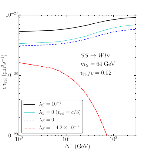
Figure 1: The cross section $\sigma v_{{\rm rel}}$ of $SS\to WW^{\ast}\to Wl\nu$ as a function of $\Delta^{\pm}$. The mass of DM is fixed to be $m_{S}=64\,\mathrm{GeV}$. Except the cyan line ($v_{{\rm rel}}=c/3$), we take a relative velocity $v_{{\rm rel}}=0.02c$ which can make a cancellation effect for $\lambda_{S}=-(s-m_{h}^{2})/(2v^{2})\simeq-4.2\times 10^{-3}$ as discussed in the main text. The black solid line, blue dashed and red dashed-dotted lines represent the values of $\lambda_{S}=10^{-3}$, $\lambda_{S}=0$ and $\lambda_{S}=-4.2\times 10^{-3}$, respectively.

Assuming a standard thermal history of our Universe, the number density of a particle with mass $m$ at the temperature $T$ can be simply presented by a Boltzmann distribution $\sim e^{-m/T}$. Under the thermal DM scenario, if the mass splittings between $S$, $A$, and $H^{\pm}$ are as small as the case considering in this analysis, the number densities of three particles at $T$ are comparable to each other and their co-annihilating processes play an important role of reducing the relic density. In this subsection, we summarize the dominant channels for annihilation and co-annihilation in the i2HDM.

Depending on the specific DM mass range, the DM annihilation is dominated by different channels. For the Higgs resonance regions, i.e. $m_{S}\simeq m_{h}/2$, the annihilations of $SS$ to SM fermions via the Higgs boson exchange are dominated, especially for the process $SS\rightarrow b\overline{b}$. The annihilation cross section in the function of the central energy $\sqrt{s}$ is given by

$$\sigma(s) = \frac{3\lambda_{S}^{2}}{8\pi}\frac{m_{f}^{2}}{\left(s-m_{h}^{2}\right)^{2}+\Gamma_{h}^{2}m_{h}^{2}}\times r^{3}(s,2m_{f})\times r(s,2m_{S}),~{}~{}\rm{where}$$

$$r(x,y) \equiv \sqrt{1-\frac{y^{2}}{x^{2}}}.$$ (19)

It is easy to see that the annihilation cross section from Eq. (III.3) is dramatically decreased when $m_{S}>m_{h}/2$.

For the region of $m_{S}>m_{h}/2$, the annihilation of $SS$ to $W^{+}W^{-(\ast)}$ via the four-vertex interaction, the $s$-channel $h$ exchange, and the $t$ and $u$-channel with $H^{\pm}$ exchange, becomes the dominant channel. The contribution from four-vertex diagram is usually dominant while the one from charged Higgs is typically small. The one from $h$ exchange becomes important only at around the Higgs resonance region. However, the total $SS\to W^{+}W^{-(\ast)}$ annihilation can be significantly reduced by the cancellations among these contributions. First, the cancellation between the four-vertex diagram and $h$ exchange contribution can take place at $\lambda_{S}=-(s-m_{h}^{2})/(2v^{2})$ Honorez:2010re . Second, if the masses of $S$ and $H^{\pm}$ are nearly degenerate, the cancellation between the four-vertex diagram and charged Higgs contribution can also occur. In Fig. 1, we show the cross section times relative velocity ($\sigma v_{{\rm rel}}$) for the process $SS\to WW^{\ast}\to Wl\nu$ as a function of $\Delta^{\pm}$ with various values of $\lambda_{S}$. The cross section is computed by using MadGraph5. The DM mass is fixed to be $m_{S}=64\,\mathrm{GeV}$ and its relative velocity in the early universe is taken as $v_{{\rm rel}}/c=0.02$ in order to realize a cancellation between the four-vertex diagram and $h$ exchange contribution for $\lambda_{S}=-(s-m_{h}^{2})/(2v^{2})\simeq-4.2\times 10^{-3}$. We also present the cyan line ($\lambda=0$ with $v_{{\rm rel}}=c/3$) as a reference. Three benchmark values of $\lambda$ are selected based on the allowed region given in a previous study Arhrib:2013ela . For a positive value of $\lambda_{S}=10^{-3}$ (black solid line), the contribution from the four-vertex diagram and s-channel Higgs exchange are dominant. When the $s$-channel Higgs exchange is removed by setting $\lambda_{S}=0$ (blue dashed line), $\sigma v_{{\rm rel}}$ is reduced but still sizable. For $\lambda_{S}=-4.2\times 10^{-3}$ (red dashed-dotted line), one can see that $\sigma v_{{\rm rel}}$ is the smallest and even can be neglected if the charged Higgs mass becomes heavy. This is due to the maximal cancellation between the four-vertex diagram and $h$ exchange contribution. The remaining $\sigma v_{{\rm rel}}$ is mainly from the charged Higgs contribution. One can also see that from the black solid and blue dashed lines, $\sigma v_{{\rm rel}}$ is slightly dropped if the mass splitting $\Delta^{\pm}$ decreases from $\sim 250$ GeV down to $\sim 1$ GeV. This is the result of the cancellation between the four-vertex diagram and $t/u$ channel charged Higgs contributions.

Unlike the most parameter space of the i2HDM, the difficulty of a compressed mass spectrum scenario is that additional co-annihilation channels in this scenario make under-abundant relic density. Ideally, the annihilation has to be properly switched off, but it is particularly hard for $SS\to WW^{(\ast)}$ because the coupling of four-vertex diagram $SSWW$ is the electroweak coupling. Therefore, the only way to reduce the annihilation cross section of $SS\to WW^{*}$ is via cancellation as shown in Fig. 1. Since the mass splitting $\Delta^{\pm}$ in this work is always greater than $1\,\mathrm{GeV}$, it is interesting to see the role of the $t/u$-channel with $H^{\pm}$ exchange playing in the cancellation. By engaging with micrOMEGAs package, we have checked that if we change $\Delta^{\pm}$ from $20\,\mathrm{GeV}$ to $500\,\mathrm{GeV}$, the relic density is slightly changed by a few percent. Hence, the $t/u$-channel with $H^{\pm}$ exchange are not the leading contribution to suppress the contribution from $SS\to WW^{\ast}$ annihilation in the co-annihilation scenario.

The co-annihilation contribution to the relic density is more complicated than the annihilation process. In particular, it depends on the size of mass splitting $\Delta^{0}$ and $\Delta^{\pm}$. Since we are focusing on the compressed mass spectrum scenario, the co-annihilation happens naturally and cannot be expelled from the full mass regions. In such a small mass splitting scenario, the most dominant co-annihilation channels are:

• $SA\to f\bar{f}$ for a small $\Delta^{0}$.

• $SH^{\pm}\to\gamma W^{\pm}$ for a small $\Delta^{\pm}$.

Unlike other subdominant co-annihilation channels, these two co-annihilation cross sections are only involved with the SM couplings. Naively speaking, the relic density in the co-annihilation dominant region is essentially controlled by the two mass splittings $\Delta^{0}$ and $\Delta^{\pm}$.

We evolve the Boltzmann equation by using the public code MicrOMEGAs Belanger:2018mqt . The numerical result of the relic density which has been taken into account the annihilation and co-annihilation contributions, is required to be in agreement with the recent PLANCK measurement Aghanim:2018eyx :

$$\Omega_{\rm{CDM}}h^{2}=0.1199\pm 0.0027.$$ (20)

We would like to comment on the multi-component DM within the framework of the i2HDM. If there exists more than one DM particle in the Universe, the DM $S$ can be only a fraction of the relic density and the DM local density. The DM constraints from relic density, direct detection, and indirect detection can be somewhat released. However, an important question followed by adding more new particles to the Lagrangian is whether the Higgs potential is altered and theoretical constraints are still validated. Such a next-to-minimal i2HDM is indeed interesting but beyond the scope of our current study. Here, we only consider the one component DM scenario.

III.4 DM direct detection

As indicated by several Higgs portal DM models Cheung:2012xb ; Athron:2017kgt ; Athron:2018hpc , the most stringent constraint on DM-SM interaction currently comes from the DM direct detection. This is also true in the case of the i2HDM, if we only consider the DM-quark/gluon elastic scattering via $t$-channel Higgs exchange at the leading order. Simply speaking, one would expect that the size of $S-S-h$ effective coupling ($\lambda_{S}$ at tree-level) can be directly constrained by the latest XENON1T experiment Aprile:2018dbl .

However, for a highly mass degenerated scenario $\Delta^{0}\simeq 0$, the DM-quark inelastic scattering $Sq\to Aq$ can be described by an unsuppressed coupling $Z-S-A$ whose size is fixed by the electroweak gauge coupling. Indeed, such the DM inelastic scattering scenario predicts a huge cross section but it has already excluded by the latest XENON1T result Arina:2009um ; Chen:2019pnt . The inelastic interactions are inefficient when the $\Delta^{0}$ is larger than the momentum exchange $\simeq\mathcal{O}(200\,\mathrm{keV})$ Arina:2009um . Hence, it is safe to ignore the inelastic interactions when requiring $\Delta^{0}\geq 10^{-3}\,\mathrm{GeV}$. We not that $\Delta^{0}$ has to be greater than $5\,\mathrm{GeV}$ when the DM relic density constraint is considered.

Going beyond the leading order calculation, we calculate the corrections at the next leading order in the i2HDM. We fold all the next leading order corrections into the effective coupling $\lambda_{S}^{\rm eff}$ which depends on the relative energy scale we have set. Once the input scales of our scan parameters are fixed at the EW scale, the effective coupling $\lambda_{S}^{\rm eff}$ will be modified at the low energy scale where the recoil energy of DM-quark/gluon scattering is located. As shown in the Appendix A, the one-loop correction $\delta\lambda$ is a function of $m_{S},\Delta^{0},\Delta^{\pm}$, and $\lambda_{2}$. Its value can be either positive or negative. Therefore, we can introduce a factor $R$ to illustrate the loop-induced effects,

$$R=\frac{\sigma^{\rm{SI}}_{p}(\texttt{tree+loop})}{\sigma^{\rm{SI}}_{p}(\texttt{tree})}=\left(\frac{\lambda_{S}+\delta\lambda}{\lambda_{S}}\right)^{2}=\left(\frac{\lambda_{S}^{\rm eff}}{\lambda_{S}}\right)^{2}.$$ (21)

The correction parameter $\delta\lambda$ is computed by using LoopTools code Hahn:1998yk . We consider two scenarios in this work: the XENON1T likelihood (Poisson distribution) is obtained with and without $R$ by using DDCalc code Workgroup:2017lvb . Note that both the tree and loop level are isospin conserving. Hence, the value of $R$ for DM-proton and DM-neutron scattering are approximately the same.

III.5 DM indirect detection

In addition to the singlet Higgs DM whose annihilation is only via SM Higgs exchange, the i2HDM at the present universe can be also dominated by the four-points interaction $SSW^{+}W^{-}$. If the DM annihilation is considerable, e.g. at dwarf spheroidal galaxies (dSphs) or galactic center where DM density is expected to be rich, some additional photons or antimatter produced by $W$ bosons or SM fermion pair would be detected by the DM indirect detection. Unfortunately, none of the indirect detection experiments reports a positive DM annihilation signal but gives a sever limit on the DM annihilation cross section. Thanks to a better measured dSphs kinematics which gives smaller systematic uncertainties than other DM indirect detection, the most reliable limit on the DM annihilation cross section at the DM mass $\sim\mathcal{O}(100\,\mathrm{GeV})$ comes from Fermi dSphs gamma ray measurements so far Fermi-LAT:2016uux .

On the other hand, several groups have found out some anomalies such as GCE Goodenough:2009gk ; Hooper:2010mq ; Calore:2014xka ; TheFermi-LAT:2017vmf and AMS02 antiproton excess Cui:2016ppb ; Cuoco:2016eej which might be able to be explained by the DM annihilation. Interestingly, these two anomalies are located at the DM mass $\sim 50-100\,\mathrm{GeV}$ region where coincides with the mass region discussed in this paper. Hence, we adopt a strategy in this work that only Fermi dSphs gamma-ray constraints are included in the scan level, but our allowed parameter space is compared with antiproton anomaly.

The differential gamma-ray flux due to the DM annihilation at the dSphs halo is given by

$$\frac{d\Phi_{\gamma}}{dE_{\gamma}}={\frac{\langle\sigma v\rangle}{8{\pi}m_{S}^{2}}\times J\times\sum_{\texttt{ch}}{\rm BR}(\texttt{ch})\times\frac{dN^{\texttt{ch}}_{\gamma}}{dE_{\gamma}}}.$$ (22)

The $J$-factor is $J={\int}dld{\Omega}{\rho}(l)^{2}$, where the integral is taken along the line of sight from the detector with the open angle $\Omega$ and the DM density distribution $\rho$. We adopt 15 dSphs and their $J$-factors as implemented in LikeDM Huang:2016pxg . We sum over all the DM annihilation channels ch. The annihilation branching ratio ${\rm BR}(\texttt{ch})$ and energy spectra $dN^{\texttt{ch}}_{\gamma}/dE_{\gamma}$ are computed by using micrOMEGAs in which the three-body final states (e.g. $SS\to WW^{*}\to W^{+}l^{-}\nu$) are properly taken into account. In this paper, we only focus on the region of $m_{S}<100\,\mathrm{GeV}$. For the DM indirect detection at the region of $m_{S}>100\,\mathrm{GeV}$, the future Cherenkov Telescope Array may give a severe limit Queiroz:2015utg .

IV Results and discussions

IV.1 Numerical method 

Likelihood type	Constraints	See text in
Step	perturbativity, stability, tree-level unitarity	Sec. III.1
	LEP-II, OPAL	Sec. III.2.2
Poisson	XENON1T (2018), Fermi dSphs $\gamma$ data	Sec.III.4, III.5
Half-Gaussian	exotic Higgs decays	Sec. III.2.3
Gaussian	relic abundance, $R_{\gamma\gamma}$, EWPT	Sec. III.3, III.3, III.2.1

Table 1: Likelihood distributions used in our analysis.

In a similar procedure developed in our previous works Arhrib:2013ela ; Cheung:2014hya ; Matsumoto:2014rxa ; Matsumoto:2016hbs ; Banerjee:2016hsk ; Matsumoto:2018acr , we use the likelihood distribution given in the Table 1 in our Markov Chain Monte Carlo scan. Considering the lower DM mass which might be potentially detected in the colliders, DM direct and indirect detections, we only focus on the DM mass less than $100\,\mathrm{GeV}$. Engaging with emcee ForemanMackey:2012ig , we perform 35 Markov chains in the five dimensional parameter space,

$$5.0 \leq\,m_{S}/\textrm{ GeV}\,\leq 100.0\;,$$

$$10^{-3} \leq\,\Delta^{0}/\textrm{ GeV}\,\leq 20\;,$$

$$1.0 \leq\,\Delta^{\pm}/\textrm{ GeV}\,\leq 30\;,$$

$$-2.0 \leq\,\lambda_{S}\,\,\leq 2.0\;,$$

$$0.0 \leq\,\lambda_{2}\,\leq 4.2\;.$$

Here, we only choose $\Delta^{\pm}$ up to $30\,\mathrm{GeV}$ but one can freely extend it to a larger value until $m_{H^{\pm}}\sim 250\,\mathrm{GeV}$ disfavored by the EWPT data (for a detailed analysis, see Ref. Bhardwaj:2019mts ). On the other hand, without the helps from the charged Higgs co-annihilations, we have checked that the total co-annihilation contribution to the relic density cannot be larger than $85\%$.

In order to scan the parameter space more efficiently, we set the range of $\lambda_{2}$ up to 4.2 allowed by the unitarity constraint Arhrib:2013ela . We compute the mass spectrum, theoretical conditions and oblique parameters by using 2HDMC. All survived parameter space points are then passed to micrOMEGAs to compute the relic density and the tree-level DM-nucleon elastic scattering cross section. The XENON1T statistics test is computed by using DDCalc. The loop corrections of DM-nucleon elastic scattering cross section is calculated by using LoopTools. In the end, we have collected more than 2.5 million data points and our achieved coverage of the parameter space is good enough to pin down the contours by using “Profile Likelihood” method Rolke:2004mj . Under the assumption that all uncertainties follow the approximate Gaussian distributions, confidence intervals are calculated from the tabulated values of $\Delta\chi^{2}\equiv-2\ln(\mathcal{L/L}_{\rm{max}})$. Thus, for a two dimension plot, the 95% confidence ($2\sigma$) region is defined by $\Delta\chi^{2}\leq 5.99$.

IV.2 Co-annihilation and mixed scenarios

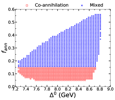
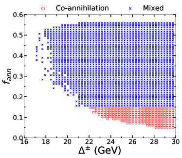
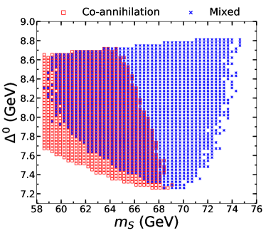
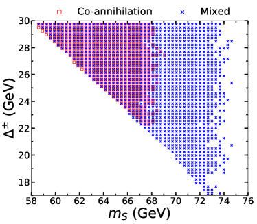
Figure 2: The $2\sigma$ allowed regions from the theoretical conditions, LEP, and PLANCK constraints. The red square and blue cross are the co-annihilation ($f_{ann}<15\%$) and mixed regions ($f_{ann}>15\%$), respectively

As mentioned in Sec. III.3, the compressed mass spectrum scenario guarantees the number density of $S$, $A$ and $H^{\pm}$ at the same temperature before freeze-out are comparable. Nevertheless, the thermal averaged cross section of co-annihilation could be very different with annihilation one. Therefore, the interaction rate can describe the effects from both the thermal averaged cross section and their mass splitting. If the interaction rate is below the Hubble expansion rate, the freeze-out mechanism occurs. Additionally, it is hard to cease the annihilation processes, particularly from four-points interactions whose the contributions are always significant at the mass region $m_{h}/2<m_{S}\lesssim 500\,\mathrm{GeV}$. Here, we introduce a new parameter $f_{ann.}$ to account for the fraction of interaction rate attributable to the annihilation. Following the convention from micrOMEGAs, the fraction $f_{ann.}$ can be given by

$$f_{ann.} = \frac{\Gamma_{ann.}}{\Gamma_{tot.}},$$ (23)

where $\Gamma_{ann.}$ and $\Gamma_{tot.}$ are the annihilation and total interaction rate before freeze-out, respectively. In this analysis, we assume that the co-annihilation domination before freeze-out acquires $f_{ann.}<0.15$.

The allowed regions of theoretical conditions, LEP, and PLANCK $2\sigma$ projected on ($\Delta^{0}$, $f_{ann.}$) and ($\Delta^{\pm}$, $f_{ann.}$) planes are shown in the two upper panels of Fig. 2. We found that the co-annihilation rate ($\Gamma_{tot.}-\Gamma_{ann.}$) is always larger than $45\%$ in our parameter space of interest. Therefore, there is no pure annihilation contribution in this compressed mass spectrum scenario. We also see that the relic density constraints can give a lower limit for both $\Delta^{0}$ and $\Delta^{\pm}$ because the co-annihilation processes are too efficient to reduce the relic density. On the other hand, $\Delta^{0}<8.7\,\mathrm{GeV}$ is caused by the LEP-II constraints. We note that there is no upper limit of $\Delta^{\pm}$ from neither OPAL exclusion nor PLANCK measurement. The small $m_{S}$ and $\Delta^{\pm}$ regions are excluded by the OPAL as shown in the right bottom panel of Fig. 2.

Once the phase space of $SS\to W^{+}W^{-(\ast)}$ process is suppressed at the early universe, the co-annihilation rate dominates $\Gamma_{tot}$ before freeze-out. As a result, the co-annihilation scenario $f_{ann.}<0.15$ only located at the region $m_{S}<70\,\mathrm{GeV}$. The annihilation process $SS\to W^{+}W^{-(\ast)}$ is still at least $5\%$ contribution to $\Gamma_{tot}$.

There are three edges of the allowed region in ($m_{S}$, $\Delta^{0}$) plane. The left-bottom and right-bottom corner are excluded by too little and too much relic density, respectively. The upper limit on the mass splitting, $\Delta^{0}\mathrel{\mathop{\kern 0.0pt\hbox to0.0pt{\raise 0.86108pt\hbox{$<$}\hss}}\lower 3.87495pt\hbox{\kern-1.90002pt$\sim$}}8.8\,\mathrm{GeV}$, is due to the LEP limit and this also leads to that $f_{ann.}\lesssim 55\%$. Therefore, the expected features of annihilation are hidden in the region of the Mixed scenario. For example, near the Higgs resonance region ($m_{S}\simeq 62\,\mathrm{GeV}$), one can see a small kink at the edge $\Delta^{0}\approx 7.6-7.7\,\mathrm{GeV}$ of the Mixed scenario region.

IV.3 Results

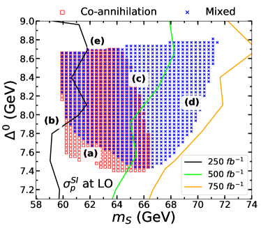
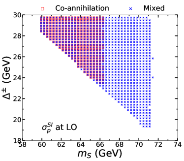
Figure 3: Left panel: the $2\sigma$ allowed regions from all constraints projected on ($m_{S}$, $\Delta^{0}$) plane. The black, green, and orange contours are the prospect of $2\sigma$ significance with the integrated luminosity of 250 ${\rm fb}^{-1}$, 500 ${\rm fb}^{-1}$, and 750 ${\rm fb}^{-1}$ for one of the signal regions in Ref. Aad:2019qnd as shown in the main text, respectively. Right panel: the $2\sigma$ allowed regions from all constraints projected on ($m_{S}$, $\Delta^{\pm}$) plane. The $\sigma^{\rm{SI}}_{p}$ is calculated at leading order and the colored codes for the scatter points are the same as Fig. 2.

In this section, we present the $2\sigma$ allowed region based on the total likelihoods, as shown in Table 1. Those constraints have been discussed in Sec. III and they are referred to the phrase “all constraints”, unless indicated otherwise.

Fig. 3 shows the $2\sigma$ allowed region by taking into account all constraints. The left panel is on the ($m_{S}$, $\Delta^{0}$) plane and the right panel is on ($m_{S}$, $\Delta^{\pm}$) plane. Here, the $\sigma^{\rm{SI}}_{p}$ is computed at LO. By comparing with the lower panels in Fig. 2, we can easily see that the allowed range of the DM mass is shrunk to $60<m_{S}/\,\mathrm{GeV}<72$ after applying all constraints. Since the correlations between $m_{S}$, $\Delta^{0}$, and $\Delta^{\pm}$ are non-trivial but important for understanding the different features of mixed scenario (blue crosses) and co-annihilation scenario (red squares), we label some specific regions shown in the left panel of Fig. 3 and discuss some features for these regions as follows:

• Region (a), the small $\Delta^{0}$ can provide an efficient co-annihilation to reach the correct relic density even without the annihilation. One has to keep in mind that the coupling $\lambda_{S}$ can be either very small or a negative value in this region. It depends on whether $SS\to WW^{\ast}$ is close (a tiny $\lambda_{S}$) or opened (a negative $\lambda_{S}$).

• Region (b), comparing with the lower panel in Fig. 2, involving the Higgs invisible decay constraint lifts the lower limit on DM mass to $60\,\mathrm{GeV}$.

• Region (c), the co-annihilation scenario cannot reach the large $m_{S}$ regions, particularly $m_{S}<64$ GeV for $\Delta^{0}=8.7$ GeV and $m_{S}<66\,\mathrm{GeV}$ for $\Delta^{0}=7.4\,\mathrm{GeV}$. This is due to the current DM direct detection constraint. In particular, a negative value of the coupling between the DM and Higgs boson is needed in the larger DM mass region so that the cancellation between $SS\to h^{\ast}\to WW^{\ast}$ and the four-points interaction $SSWW$ can occur to satisfy the relic abundance. However, this enhances $\sigma^{\rm{SI}}_{p}$ to be excluded by the XENON1T measurements. We also note that, due to the OPAL exclusion, a smaller DM mass region results in a larger $\Delta^{\pm}$ value. For the co-annihilation scenario, one can see that $\Delta^{\pm}>23\,\mathrm{GeV}$ as shown in the right panel of Fig. 3.

• Region (d), it is totally opposite to the region (a). The relic density at this region mainly comes from $SS\to W^{\pm}W^{\mp(\ast)}$ annihilation. Therefore, $\Delta^{0}$ shall be large enough to suppress co-annihilation and its lower bound is varied with respect to $m_{S}$. The mixed scenario can reach a larger DM mass region as compared with the co-annihilation scenario. On the other hand, the lower limit of $\Delta^{\pm}$ for the mixed scenario from the OPAL exclusion is more released. As shown in the right panel of Fig. 3, the mass splitting $\Delta^{\pm}\mathrel{\mathop{\kern 0.0pt\hbox to0.0pt{\raise 0.86108pt\hbox{$>$}\hss}}\lower 3.87495pt\hbox{\kern-1.90002pt$\sim$}}19$ GeV for the mixed scenario.

• Region (e), the LEP-II exclusion is presented. Together with the current XENON1T constraint, they yield two important upper limits: $\Delta^{0}<8.8\,\mathrm{GeV}$ and $m_{S}<72\,\mathrm{GeV}$.

As mentioned in the previous section, the current searches at the LHC is not yet to bite the parameter space. However, we find that the extended searches at the LHC Run 3, especially for the compressed mass spectra searches, can probe both co-annihilation and mixed scenarios. On the left panel of Fig. 3, we show the future prospect contours of 2$\sigma$ significance from the LHC compressed mass spectra searches with the integrated luminosity of 250 ${\rm fb}^{-1}$ (black line), 500 ${\rm fb}^{-1}$ (green line), and 750 ${\rm fb}^{-1}$ (orange line). Here, we fix $\lambda_{S}=0$, $\lambda_{2}=1$ and $\Delta^{\pm}=28\,\mathrm{GeV}$ as a benchmark point and only recast the dimuons final state of SR-E-low signal region with the muons invariant mass window: 3.2 GeV $\leq m_{\mu^{+}\mu^{-}}\leq$ 5 GeV Aad:2019qnd . The significance is given by $z=S/\sqrt{B+\delta_{B}^{2}}$, where $S$ is the number of signal event, $B$ is the number of background event and $\delta_{B}$ is the background uncertainty which is assumed to be $10\%$ of the number of background event at the future LHC. One can see that both scenarios can be partly probed at the LHC Run 3 with ${\cal{L}}$ = 250 ${\rm fb}^{-1}$. The parameter space in the co-annihilation scenario can be mostly covered if the integrated luminosity reach 500 ${\rm fb}^{-1}$, while one needs the luminosity about 750 ${\rm fb}^{-1}$ to probe the whole parameter space in the mixed scenario. A combined analysis of various signal regions, as the strategy presented in Ref. Aad:2019qnd , will certainly improve the significance, however, it is beyond the scope of this work. On the other hand, the mass-splitting $\Delta^{\pm}$ is sensitive to the stransverse mass $m_{T2}$, similar recasting method can be done according to Ref. Aad:2019qnd . We will return to these two parts in a future work.

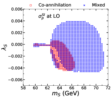
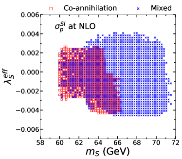
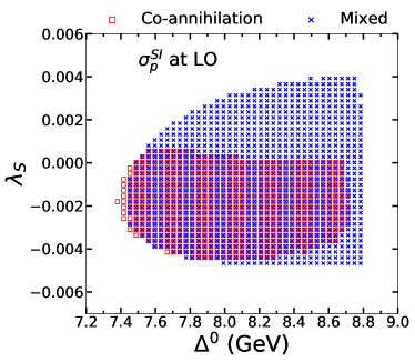
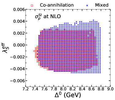
Figure 4: The scatter plots in $2\sigma$ allowed region. Left panels indicate the $\sigma^{\rm{SI}}_{p}$ computed at LO while right panels represent the $\sigma^{\rm{SI}}_{p}$ computed at NLO. Note that the effective coupling $\lambda_{S}^{\rm eff}=\lambda_{S}+\delta\lambda$ in the right panels. The color scheme is the same as Fig. 2.

As shown in Eq. (21), the NLO effects on the DM-proton scattering cross section can be understood by comparing the $\lambda_{S}$ and $\lambda_{S}^{\rm eff}$ couplings. In Fig. 4, we show the $2\sigma$ allowed region taking into account all constraints. The elastic scattering cross section $\sigma^{\rm{SI}}_{p}$ in the two left panels are based on the tree level coupling $\lambda_{S}$, and the two right panels are based on $\lambda_{S}^{\rm eff}$. Let us start with the two upper panels of Fig. 4. We can see two interesting regions: i) $m_{S}\lesssim m_{h}/2$, and ii) $m_{S}\gtrsim m_{h}/2$. Because of the Higgs resonance or co-annihilation process in the early universe, the $\lambda_{S}$ of the first region is required to be small to fulfill the relic density constraint, however such a small coupling makes an undetectable $\sigma^{\rm{SI}}_{p}$ in the present XENON1T experiment. Particularly, the $\lambda_{S}$ in the co-annihilation region can be even smaller than the one in the annihilation (Higgs resonance) region. However, the NLO corrections can enhance $\sigma^{\rm{SI}}_{p}$ to be more detectable in the near future direct detection experiments, and thus the effective coupling $|\lambda_{S}^{\rm eff}|$ can reach about $0.003$ as seen in the upper right panel. Note that $\lambda_{S}^{\rm eff}$ can be generated by gauge boson loops as the $g^{2}g^{\prime 2}$ term shown in Eq. (7) from one-loop RGEs. This reveals that some fine-tuning of the parameters is needed in order to reach a tiny $|\lambda_{S}^{\rm eff}|$ which is much less than $\mathcal{O}(10^{-3})$ in Fig. 4.

Regarding the second region $m_{S}\gtrsim m_{h}/2$, the four-vertex diagram $SSWW$ process becomes too sufficient to reduce the relic density. Hence, $\lambda_{S}$ needs to be negative so that a cancellation between this diagram and $SS\to h^{\ast}\to WW^{\ast}$ can occur. We can see that the exact cancellation happens at the strip region, $\lambda_{S}\approx-(s-m_{h}^{2})/(2v^{2})$, where the mixed scenario is absent because the universe is over abundant. Once the co-annihilation mechanism is triggered, the correct relic density can be still obtained in this region and nearby. For co-annihilation scenario, the above cancellation also makes an upper bound of DM mass with respect to the size of $\lambda_{S}$.

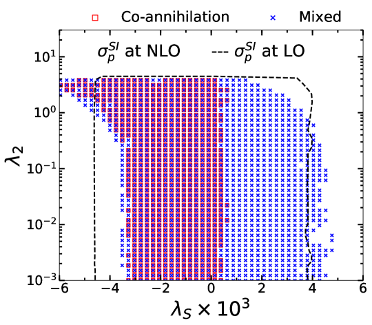
Figure 5: The scatter plots in $2\sigma$ allowed region on the plane of ($\lambda_{S}\times 10^{3}$, $\lambda_{2}$). The scattered points represent $\sigma^{\rm{SI}}_{p}$ at NLO while the region inside black dashed contours indicates that $\sigma^{\rm{SI}}_{p}$ is computed at LO.

The two lower panels of Fig. 4 show the $2\sigma$ distribution of $\lambda_{S}$ (left panel) and $\lambda_{S}^{\rm eff}$ (right panel) as a function of $\Delta^{0}$. The maximum value of $\Delta^{0}$ for co-annihilation scenario is due to the combined constraints from LEP-II and relic density. Because a large positive value of $\lambda_{S}$ in this scenario is disfavored when the $SS\to WW^{*}$ annihilation process kinematically opens, the asymmetry between positive and negative $\lambda_{S}$ can be found in the co-annihilation scenario. In addition, the co-annihilation gradually losses the power if splitting $\Delta^{0}$ increases and therefore the positive $\lambda_{S}$ has to be decreased once co-annihilation dominates at the early universe. However, the negative $\lambda_{S}$ is rather favorable because of the cancellation between diagrams of the four-points interaction and $SS\to h^{\ast}\to WW^{\ast}$. Again, we can see from the lower-right panel that the NLO corrections can generally increase the size of $|\lambda_{S}^{\rm eff}|$, especially for the positive $\lambda_{S}$ region which has been excluded if only tree level is considered. Note that the value of $|\lambda_{S}^{\rm eff}|$ can be smaller than $|\lambda_{S}|$ if the loop correction parameter $\delta\lambda$ and $\lambda_{S}$ are opposite signs as shown in Appendix B.

In Fig. 5, the NLO effects are more distinguishable on the plane of ($\lambda_{S}\times 10^{3}$, $\lambda_{2}$). The coupling $\lambda_{2}$ is not involved in LO processes, but it causes some interesting behaviors once the NLO corrections are included. There are two main features. The first feature is that some cancellations between the tree level diagrams and loop level diagrams are taking place. Particularly, these tree-loop cancellations can be found in the region of $\lambda_{S}\mathrel{\mathop{\kern 0.0pt\hbox to0.0pt{\raise 0.86108pt\hbox{$<$}\hss}}\lower 3.87495pt\hbox{\kern-1.90002pt$\sim$}}-4.8\times 10^{-4}$ and $\lambda_{2}>1$ as well as the region $\lambda_{S}>4\times 10^{-4}$ where the parameter space were excluded from LO computation but they can be saved when including NLO corrections. The second feature is that the NLO contribution generally increases $\sigma^{\rm{SI}}_{p}$. Apart from the tree-loop cancellation region, more parameter space have been ruled out comparing with only LO computation.

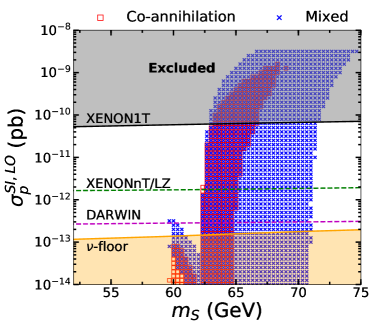
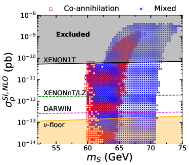
Figure 6: The scatter plots on the ($m_{S}$, $\sigma^{\rm SI}_{p}$) plane. Allowed points are in $2\sigma$ agreement with all constrains except the XENON1T measurements. The DM-proton scattering cross section is computed at LO in the left panel while the one taking into account the one loop correction is presented in the right panel. The color scheme for the scatter points is the same as Fig. 2. The solid black line represents the limit from XENON1T Aprile:2018dbl . The projected sensitivities of LZ Akerib:2015cja and DARWIN Aalbers:2016jon are dashed green and dashed magenta lines, respectively. The orange region is the neutrino background Billard:2013qya .

Fig. 6 shows the DM-proton scattering cross section as a function of DM mass, $m_{S}$, at tree-level (left panel) and one-loop level (right panel). Note that the DM direct detection constraints are not included in the scatter point regions to demonstrate its exclusion power. Again, the inelastic scattering can be neglected at the region $\Delta^{0}\gtrsim\mathcal{O}(200\,\mathrm{keV})$ Arina:2009um . Hence, the only significant contribution to the detection rate is the elastic scattering via $t$-channel Higgs exchange.

Because both scenarios are generally required a small $\lambda_{S}$ to fulfill the relic density constraints, making a drawback to detect the co-annihilation and Higgs resonance region. In the left panel, we can see that the elastic scattering cross section in the resonance region, $m_{S}\mathrel{\mathop{\kern 0.0pt\hbox to0.0pt{\raise 0.86108pt\hbox{$<$}\hss}}\lower 3.87495pt\hbox{\kern-1.90002pt$\sim$}}m_{h}/2$, is overall lower than the future projected sensitivities from LZ Akerib:2015cja and DARWIN Aalbers:2016jon . The co-annihilation region at $m_{S}<m_{h}/2$ is even below the neutrino floor and hard to be detected under current strategies of DM direct detection.

Strikingly, once the next-leading order correction for $\sigma^{\rm{SI}}_{p}$ is considered, the elastic scattering cross section $\sigma^{\rm{SI}}_{p}$ in the Higgs resonance and the co-annihilation regions are both significantly enhanced. Thanks to the loop contributions, especially from the large $|\lambda_{2}|$, co-annihilation region can be testable in the future direct detection searches.

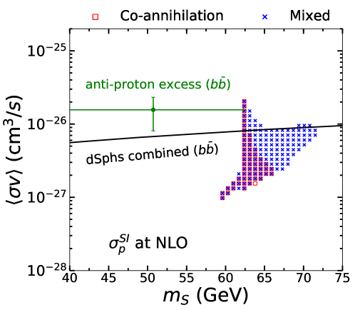
Figure 7: The scatter plots in $2\sigma$ allowed region on the ($m_{S}$, $\langle\sigma v\rangle$) plane. The color scheme for the scatter points is the same as Fig. 2. The solid black line represents the combined limit for DM annihilating into $b\bar{b}$ from observations of dSphs by Fermi-LAT, HAWC, HESS, MAGIC and VERITAS Oakes:2019ywx . The green error bar is the $1\sigma$ signal region for the antiproton excess Cui:2018nlm .

Lastly, we would like to discuss the detection of the DM annihilation at the present. In Fig. 7, we show the $2\sigma$ distribution in ($m_{S}$, $\langle\sigma v\rangle$) plane, allowed by all constraints in Table 1. With a conservative treatment, we have taken only the Fermi 15 dSphs gamma ray data into our total likelihood. However, we also show the current most stringent limit (solid black line) which is obtained by combing the latest data from Fermi-LAT, HAWC, HESS, MAGIC and VERITAS Oakes:2019ywx . To illustrate the antiproton anomaly, we also present the signal region for $b\bar{b}$ final state Cui:2018nlm as a comparison.

For the region of $m_{S}<m_{h}/2$, the dominant annihilation channel is $SS\to h\to b\bar{b}$ where $\lambda_{S}$ is suppressed due to the relic density constraint. Thus, the velocity averaged cross section at this region is a relatively small value, $\langle\sigma v\rangle$ $\sim 10^{-27}~{}{\rm cm}^{3}s^{-1}$. The Higgs resonance presents at the region of $m_{S}\simeq m_{h}/2$, but the large cross section part can be excluded if one takes into account the combined limit (black line). The DM annihilation at the present universe with mass $m_{S}>m_{h}/2$ are almost entirely to $WW^{*}$ final state and its spectrum $dN/dE$ is similar to the $b\bar{b}$ final state. Except a small part of blue crosses (mixed scenario), most of parameter space in this region are still survived. Interestingly, the viable regions of the model including the mixed and co-annihilation scenarios are in agreement with the antiproton anomaly within $3\sigma$ Cui:2018nlm . Hence, if the antiproton anomaly would be confirmed in the future, one would expect to see a signal at this DM mass region from the future HL-LHC compressed mass spectrum searches.

V Summary and future prospect

The compressed mass spectrum in the i2HDM is an interesting topic. It can escape from most of current collider constraints and its relic density in this region can be mainly governed by the $S$ and $A$ co-annihilations. To obtain the correct relic density and minimize the contribution from annihilation channels, there are two main features of the co-annihilation scenario. The first one is the requirement for a negligible $|\lambda_{S}|$ near the Higgs resonance region. As a type of Higgs portal DM model, one can intuitively reduce $\lambda_{S}$ to minimize the annihilation contributions. However, this method only works at the region where $SS\to W^{+}W^{-\ast}$ is not open. Once this channel is kinematically-allowed at the early universe, the $SSW^{+}W^{-}$ four-points interaction is very sufficient to reduce the relic density. To lower down the contribution from the $SSW^{+}W^{-}$ four-points interaction, one has to choose a negative sign of $\lambda_{S}$ to make a cancellation among four-points interaction and $s$-channel Higgs exchange. Therefore, the second feature is that a negative $\lambda_{S}$ is needed if $SS\to W^{+}W^{-\ast}$ channel is kinematically-allowed at the early universe.

Because of a small or negative $\lambda_{S}$, the NLO corrections for DM-nucleon elastic scattering become more important. We first fix the input scales of our scan parameters at the EW scale, the effective coupling $\lambda_{S}^{\rm eff}$ will be modified from quantum corrections at the low energy DM direct detection scale. At the tree-level, a small value of $|\lambda_{S}|$ predicts a cross section $\sigma^{\rm{SI}}_{p}$ smaller than the neutrino floor. However, it can be testable if $\sigma^{\rm{SI}}_{p}$ includes the NLO corrections. If the value of $|\lambda_{S}|$ is large and $\lambda_{S}$ is negative, a cancellation between LO and NLO contribution may be needed in order to escape from the present XENON1T constraint. Such a NLO contribution is sensitive to not only the mass splitting $\Delta^{\pm}$ but also the coupling $\lambda_{2}$. Interestingly, the coupling $\lambda_{2}$ plays no role at the tree-level phenomenology, neither Higgs nor DM.

Motivated by the non-trivial correlations between compressed mass spectra, co-annihilations, and NLO corrections of $\sigma^{\rm{SI}}_{p}$, we conduct a global scan to comprehensively explore the parameter space of compressed mass spectra in the i2HDM, including five parameters ($m_{S}$, $\Delta^{0}$, $\Delta^{\pm}$, $\lambda_{2}$, $\lambda_{S}$) at the EW scale. Particularly, the parameters $\Delta^{0}$ and $\Delta^{\pm}$ are adopted for searching the compressed mass spectrum and co-annihilation scenario. By using the profile likelihood method, the survived parameter space were subjected to constraints from the theoretical conditions (perturbativity, stability, and tree-level unitarity), the collider limits (electroweak precision tests, LEP, and LHC), the relic density as measured by PLANCK, the $\sigma^{\rm{SI}}_{p}$ limit from XENON1T, and the $\langle\sigma v\rangle$ limit from Fermi dSphs gamma ray data. For the computation of $\sigma^{\rm{SI}}_{p}$, the LO and NLO calculations are considered separately in the likelihood. We have shown the $2\sigma$ allowed points grouped by co-annihilation scenario ($f_{ann}<15\%$) and mixed scenario ($f_{ann}>15\%$) in two dimensional projections of the parameter space.

We found that the viable parameter spaces for the co-annihilation scenario are located at the $60\,\mathrm{GeV}\lesssim m_{S}\lesssim 66\,\mathrm{GeV}$, $7.4\,\mathrm{GeV}\lesssim\Delta^{0}\lesssim 8.7\,\mathrm{GeV}$, and $\Delta^{\pm}\gtrsim 23.0\,\mathrm{GeV}$. The NLO correction $\delta\lambda$ is sensitive to $\lambda_{2}$ when it is greater than 0.2 while the contribution from $\Delta^{\pm}$ dominates the $\delta\lambda$ if $\lambda_{2}<0.2$. Due to the interplay between OPAL exclusion and PLANCK relic density constraint, the co-annihilation scenario cannot be realized with the condition $-10^{-3}\lesssim\delta\lambda\lesssim 0.0$ when the contribution from $\Delta^{\pm}$ dominates the $\delta\lambda$.

Next, the correlation between $\lambda_{S}$ and $\lambda_{2}$ is non-trivial at the NLO level. For $\lambda_{2}>1$, the same sign between $\lambda_{S}$ and $\delta\lambda$ can enhance $\sigma^{\rm{SI}}_{p}$ so that the parameter space with a large value of $\lambda_{S}$ and $\lambda_{2}$ is excluded. For $\lambda_{2}<1$, the $\Delta^{\pm}$ plays the role to NLO corrections. Therefore, the cross section $\sigma^{\rm{SI}}_{p}$ for co-annihilation scenario can be significantly enhanced but ruled out by XENON1T. It becomes testable in the future direct detection experiments.

Finally, the $95\%$ allowed region predicted in the model coincides with the AMS-02 antiproton anomaly within $3\sigma$ range. This region can be also tested by the compressed mass spectra searches at the LHC. Although we found that the region is not sensitive to the current LHC searches, it can be partially probed with future luminosity 250 ${\rm fb}^{-1}$ and mostly probed with luminosity 750 ${\rm fb}^{-1}$ as shown in the left panel of Fig. 3.

Appendix A Spin-independent cross section at the next leading order

In this Appendix, we outline the calculations of spin-independent cross section at the next leading order from Ref. Abe:2015rja . We have checked the consistency of our numerical results. First, the effective interaction of the dark matter and quark/gluon can be represented as

$${\cal L}_{\rm eff.}= \frac{1}{2}\sum_{q=u,d,s}\Gamma^{q}S^{2}(m_{q}\bar{q}q)-\frac{1}{2}\frac{\alpha_{s}}{4\pi}\Gamma^{G}S^{2}G^{a}_{\mu\nu}G^{a\mu\nu}$$

$$+\frac{1}{2m_{S}^{2}}\sum_{q=u,d,s,c,b}\left[(\partial^{\mu}S)(\partial^{\nu}S)\Gamma^{q}_{\text{t2}}{\cal O}^{q}_{\mu\nu}-S(\partial^{\mu}\partial^{\nu}S)\Gamma^{\prime q}_{\text{t2}}{\cal O}^{q}_{\mu\nu}\right],$$ (24)

where ${\cal O}^{q}_{\mu\nu}$ is the quark twist-2 operator with the following form,

$${\cal O}^{q}_{\mu\nu}\equiv\frac{i}{2}\bar{q}\left(\partial_{\mu}\partial_{\nu}+\partial_{\nu}\partial_{\mu}-\frac{1}{2}g_{\mu\nu}\not{\partial}\right)q.$$ (25)

The higher twist gluon operators have been neglected in the above effective Lagrangian. Based on Eq. (24), the scattering amplitude and spin-independent cross section of dark matter and nucleon can be written as,

$$i{\cal M}= im_{N}\left[\sum_{q}\Gamma^{q}f_{q}+\frac{2}{9}\Gamma^{G}f_{g}+\frac{3}{4}\sum_{q}(\Gamma^{q}_{\text{t2}}+{\Gamma^{\prime}}^{q}_{\text{t2}})(q(2)+\bar{q}(2))\right],$$ (26)

$$\sigma_{\text{SI}}= \frac{\mu^{2}}{4\pi m_{S}^{2}}|{\cal M}|^{2},$$ (27)

where $\mu$ is the reduced mass with the form $\mu\equiv m_{S}m_{N}/(m_{S}+m_{N})$. $m_{S}$ and $m_{N}$ are dark matter and nucleon masses, respectively.

	$\Gamma^{q}_{\text{Box}}$	$\Gamma^{q}_{\text{t2}}+{\Gamma^{\prime}}^{q}_{\text{t2}}$	$\delta\Gamma_{h}$	$\Gamma^{G}_{\text{Box}}$
$W$	$(B.5)-(B.7)$	$(B.6)$	$(C.9)-(C.16)$	$(D.19)$
$Z$	$(B.2)-(B.4)$	$(B.3)$	$(C.1)-(C.8)$	$(D.20)$

Table 2: The relevant equation numbers to calculate Feynman diagrams with effective interaction of the dark matter and quark/gluon at the next leading order from Ref. Abe:2015rja . Here $(B.5)$ means equation $(B.5)$ in Ref. Abe:2015rja with the $W$ boson contribution inside the one-loop box type diagram, for example.

At the leading order, only $\Gamma^{q}$ and $\Gamma^{G}$ are non-zero in Eq. (26) and can be given as,

$$\Gamma^{q}=\Gamma^{G}=\frac{\lambda_{S}}{m_{h}^{2}}$$ (28)

At the next leading order, we closely follow the calculations in Ref. Abe:2015rja with the following classifications,

• One-loop box type diagrams

• One-loop Higgs vertex correction diagrams

• Two-loop gluon contribution diagrams

We list relevant equation numbers to calculate above diagrams from Ref. Abe:2015rja in the Table 2. Here $(B.5)$ means equation $(B.5)$ in Ref. Abe:2015rja with the $W$ boson contribution inside the one-loop box type diagram, for example.

We can further define $\Gamma^{q}$ and $\Gamma^{G}$ at the next leading order as,

$$\Gamma^{q}=\frac{\delta\Gamma_{h}(0)}{m_{h}^{2}}+\Gamma_{\text{Box}}^{q},\qquad\Gamma^{G}=\frac{\delta\Gamma_{h}(0)}{m_{h}^{2}}+\Gamma_{\text{Box}}^{g}.$$ (29)

Finally, according to Eq.$(3.21)-(3.24)$ in Ref. Abe:2015rja and arguments therein, the one-loop correction $\delta\lambda$ are combination of functions in the Table 2 with the following form,

$$\delta\lambda\equiv \delta\Gamma_{h}(0)-\delta\Gamma_{h}(m_{h}^{2})+\frac{m_{h}^{2}}{f_{N}}\left(\sum_{q}\Gamma^{q}_{\text{Box}}f_{q}\right)+\frac{2}{9}\frac{m_{h}^{2}}{f_{N}}\Gamma^{G}_{\text{Box}}f_{g}+\frac{3}{4}\frac{m_{h}^{2}}{f_{N}}\sum_{q}(\Gamma^{q}_{\text{t2}}+{\Gamma^{\prime}}^{q}_{\text{t2}})(q(2)+\bar{q}(2)).$$ (30)

where $f_{q}$, $f_{g}$, $q(2)$ and $\bar{q}(2)$ are matrix elements for nucleons and $f_{N}\equiv\frac{2}{9}+\frac{7}{9}\sum_{q}f_{q}$. Their exact values for proton and neutron are taken from the default values of MicrOMEGAs Belanger:2018mqt . Therefore, the loop-induced effects can be simply written as the form in Eq.(21) with four input parameters : $m_{S}$, $\Delta^{0}$, $\Delta^{\pm}$ and $\lambda_{2}$ inside $\delta\lambda$.

Appendix B Supplemental figures

In this Appendix, we show some plots which are useful to understand the details of NLO effects in the parameter space.

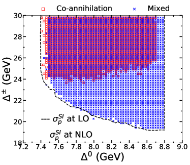
Figure 8: The scatter plots in $2\sigma$ allowed region on the plane of ($\Delta^{0}$, $\Delta^{\pm}$). The scattered points represent $\sigma^{\rm{SI}}_{p}$ at NLO while the region inside black dashed contours indicates that $\sigma^{\rm{SI}}_{p}$ is computed at LO. The color scheme is the same as Fig. 2.

The $2\sigma$ distribution for $(\Delta^{0},\Delta^{\pm})$ planes are shown in Fig. 8. The black dashed line represents $2\sigma$ contour for the LO calculation while the scatter points correspond to the one taking into account the NLO effects. From the left panel of Fig. 8, one can see that the NLO contribution takes effect only to the small $\Delta^{0}$ or $\Delta^{\pm}$ region, but it does not change the LO result significantly.

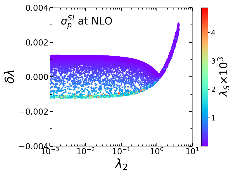
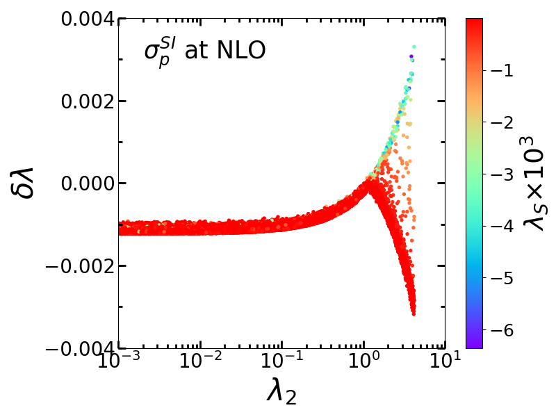
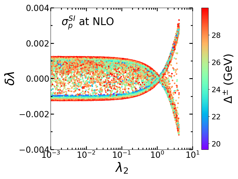
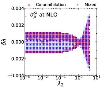
Figure 9: The $2\sigma$ allowed region on the plane ($\lambda_{2}$, $\delta\lambda$). Here, $\sigma^{\rm{SI}}_{p}$ is calculated at next leading order.

In Fig. 9, we discuss the loop correction parameter $\delta\lambda$ as a function of $\Delta^{\pm}$, $\lambda_{S}$, and $\lambda_{2}$. Although the $\Delta^{0}$ can alter the size of $\delta\lambda$, it is not significant due to its smallness required by the relic density constraint. In the two upper frames of Fig. 9, we discuss the cases of $\lambda_{S}>0$ (upper-left panel) and $\lambda_{S}<0$ (upper-right panel) on the ($\lambda_{2}$, $\delta\lambda$) plane, separately. The cross section $\sigma^{\rm{SI}}_{p}$ is proportional to the effective coupling squared $(\lambda_{S}^{\rm eff})^{2}$ which is sensitive to the relative signs of $\lambda_{S}$ and $\delta\lambda$ if they are in the same order. In particular, the cross section at NLO can even be lower than LO if the cancellation between $\lambda_{S}$ and $\delta\lambda$ occurs. A large value of $|\lambda_{S}|$ tends to accompany with an opposite sign of $\delta\lambda$, while a small value of $|\lambda_{S}|$ can either accompany with a same sign or opposite sign of $\delta\lambda$. Such a configuration results a small $\sigma^{\rm{SI}}_{p}$ at NLO as well as escapes from the XENON1T constraint.

The scatter plots of all allowed points on the ($\lambda_{2}$, $\delta\lambda$) plane are shown in the lower frames of Fig. 9. The color codes indicate the value of $\Delta^{\pm}$ (lower-left panel) and the governed relic density channels (lower-right panel). For the region of $\lambda_{2}>0.2$, the loop correction parameter $\delta\lambda$ highly depends on $\lambda_{2}$. Especially, due to the cancellation between loop diagrams, $\delta\lambda$ drops down at $\lambda_{2}\sim 1.4$. However, it significantly increases for a larger value of $\lambda_{2}$. On the other hand, $\Delta^{\pm}$ plays a significant role in $\delta\lambda$ for the region of $\lambda_{2}\mathrel{\mathop{\kern 0.0pt\hbox to0.0pt{\raise 0.86108pt\hbox{$<$}\hss}}\lower 3.87495pt\hbox{\kern-1.90002pt$\sim$}}0.2$. In particular, the lower limit on $\Delta^{\pm}$ which is due to the OPAL exclusion, can give a lower limit on the loop correction $\delta\lambda$. Furthermore, in this region, $|\delta\lambda|$ is restricted to be small ($|\delta\lambda|<1.1\times 10^{-3}$) due to our choice of $\Delta^{\pm}<$ 30 GeV. As aforementioned, the OPAL exclusion is more stringent on the co-annihilation than the mixed scenario, hence a stronger lower limit on $|\delta\lambda|$ is set for the co-annihilation scenario. This results in the blank strip for the co-annihilation scenario (red crosses) appears at around the region $-10^{-3}<\delta\lambda<0$. We note that the loop correction $|\delta\lambda|$ is slightly larger for the mixed scenario in the region $\lambda_{2}\mathrel{\mathop{\kern 0.0pt\hbox to0.0pt{\raise 0.86108pt\hbox{$>$}\hss}}\lower 3.87495pt\hbox{\kern-1.90002pt$\sim$}}1.4$.

References

- (1) R. Bernabei et al. [DAMA and LIBRA Collaborations], Eur. Phys. J. C 67 (2010) 39 doi:10.1140/epjc/s10052-010-1303-9 [arXiv:1002.1028 [astro-ph.GA]].
- (2) C. E. Aalseth et al. [CoGeNT Collaboration], Phys. Rev. Lett. 106 (2011) 131301 doi:10.1103/PhysRevLett.106.131301 [arXiv:1002.4703 [astro-ph.CO]].
- (3) M. Ackermann et al. [Fermi-LAT Collaboration], Astrophys. J. 840 (2017) no.1, 43 doi:10.3847/1538-4357/aa6cab [arXiv:1704.03910 [astro-ph.HE]].
- (4) M. Y. Cui, Q. Yuan, Y. L. S. Tsai and Y. Z. Fan, Phys. Rev. Lett. 118 (2017) no.19, 191101 doi:10.1103/PhysRevLett.118.191101 [arXiv:1610.03840 [astro-ph.HE]].
- (5) A. Cuoco, M. Kramer and M. Korsmeier, Phys. Rev. Lett. 118 (2017) no.19, 191102 doi:10.1103/PhysRevLett.118.191102 [arXiv:1610.03071 [astro-ph.HE]].
- (6) M. Felcini, arXiv:1809.06341 [hep-ex].
- (7) F. Richard, G. Arcadi and Y. Mambrini, Eur. Phys. J. C 75 (2015) 171 doi:10.1140/epjc/s10052-015-3379-8 [arXiv:1411.0088 [hep-ex]].
- (8) T. Han, S. Mukhopadhyay and X. Wang, Phys. Rev. D 98 (2018) no.3, 035026 doi:10.1103/PhysRevD.98.035026 [arXiv:1805.00015 [hep-ph]].
- (9) G. Arcadi, M. Dutra, P. Ghosh, M. Lindner, Y. Mambrini, M. Pierre, S. Profumo and F. S. Queiroz, Eur. Phys. J. C 78 (2018) no.3, 203 doi:10.1140/epjc/s10052-018-5662-y [arXiv:1703.07364 [hep-ph]].
- (10) K. Griest and D. Seckel, Phys. Rev. D 43 (1991) 3191. doi:10.1103/PhysRevD.43.3191
- (11) L. A. Harland-Lang, V. A. Khoze, M. G. Ryskin and M. Tasevsky, JHEP 1904 (2019) 010 doi:10.1007/JHEP04(2019)010 [arXiv:1812.04886 [hep-ph]].
- (12) N. Okada and O. Seto, Phys. Rev. D 101 (2020) no.2, 023522 doi:10.1103/PhysRevD.101.023522 [arXiv:1908.09277 [hep-ph]].
- (13) N. G. Deshpande and E. Ma, Phys. Rev. D 18 (1978) 2574. doi:10.1103/PhysRevD.18.2574
- (14) E. Ma, Phys. Rev. D 73 (2006) 077301 doi:10.1103/PhysRevD.73.077301 [hep-ph/0601225].
- (15) R. Barbieri, L. J. Hall and V. S. Rychkov, Phys. Rev. D 74 (2006) 015007 doi:10.1103/PhysRevD.74.015007 [hep-ph/0603188].
- (16) L. Lopez Honorez, E. Nezri, J. F. Oliver and M. H. G. Tytgat, JCAP 0702 (2007) 028 doi:10.1088/1475-7516/2007/02/028 [hep-ph/0612275].
- (17) N. Blinov, J. Kozaczuk, D. E. Morrissey and A. de la Puente, Phys. Rev. D 93 (2016) no.3, 035020 doi:10.1103/PhysRevD.93.035020 [arXiv:1510.08069 [hep-ph]].
- (18) A. Arhrib, Y. L. S. Tsai, Q. Yuan and T. C. Yuan, JCAP 1406 (2014) 030 doi:10.1088/1475-7516/2014/06/030 [arXiv:1310.0358 [hep-ph]].
- (19) J.-M. Gerard and M. Herquet, Phys. Rev. Lett. 98 (2007) 251802 doi:10.1103/PhysRevLett.98.251802 [hep-ph/0703051 [HEP-PH]].
- (20) N. Aghanim et al. [Planck Collaboration], arXiv:1807.06209 [astro-ph.CO].
- (21) T. Abe and R. Sato, JHEP 1503 (2015) 109 doi:10.1007/JHEP03(2015)109 [arXiv:1501.04161 [hep-ph]].
- (22) A. Goudelis, B. Herrmann and O. Stal, JHEP 1309 (2013) 106 doi:10.1007/JHEP09(2013)106 [arXiv:1303.3010 [hep-ph]].
- (23) M. Cirelli, N. Fornengo and A. Strumia, Nucl. Phys. B 753 (2006) 178 doi:10.1016/j.nuclphysb.2006.07.012 [hep-ph/0512090].
- (24) D. Eriksson, J. Rathsman and O. Stal, Comput. Phys. Commun. 181 (2010) 189 doi:10.1016/j.cpc.2009.09.011 [arXiv:0902.0851 [hep-ph]].
- (25) M. E. Peskin and T. Takeuchi, Phys. Rev. D 46 (1992) 381. doi:10.1103/PhysRevD.46.381
- (26) A. Ilnicka, M. Krawczyk and T. Robens, Phys. Rev. D 93 (2016) no.5, 055026 doi:10.1103/PhysRevD.93.055026 [arXiv:1508.01671 [hep-ph]].
- (27) E. J. Chun, Z. Kang, M. Takeuchi and Y. L. S. Tsai, JHEP 1511 (2015) 099 doi:10.1007/JHEP11(2015)099 [arXiv:1507.08067 [hep-ph]].
- (28) K. A. Olive et al. [Particle Data Group], Chin. Phys. C 38 (2014) 090001. doi:10.1088/1674-1137/38/9/090001
- (29) M. Aoki, S. Kanemura and H. Yokoya, Phys. Lett. B 725 (2013) 302 doi:10.1016/j.physletb.2013.07.011 [arXiv:1303.6191 [hep-ph]].
- (30) J. Kalinowski, W. Kotlarski, T. Robens, D. Sokolowska and A. F. Zarnecki, JHEP 1812 (2018) 081 doi:10.1007/JHEP12(2018)081 [arXiv:1809.07712 [hep-ph]].
- (31) E. Dolle, X. Miao, S. Su and B. Thomas, Phys. Rev. D 81 (2010) 035003 doi:10.1103/PhysRevD.81.035003 [arXiv:0909.3094 [hep-ph]].
- (32) A. Pierce and J. Thaler, JHEP 0708 (2007) 026 doi:10.1088/1126-6708/2007/08/026 [hep-ph/0703056 [HEP-PH]].
- (33) G. Abbiendi et al. [OPAL Collaboration], Eur. Phys. J. C 32 (2004) 453 doi:10.1140/epjc/s2003-01466-y [hep-ex/0309014].
- (34) M. Acciarri et al. [L3 Collaboration], Phys. Lett. B 472 (2000) 420 doi:10.1016/S0370-2693(99)01388-X [hep-ex/9910007].
- (35) E. Lundstrom, M. Gustafsson and J. Edsjo, Phys. Rev. D 79 (2009) 035013 doi:10.1103/PhysRevD.79.035013 [arXiv:0810.3924 [hep-ph]].
- (36) M. Aaboud et al. [ATLAS Collaboration], Phys. Rev. Lett. 122 (2019) no.23, 231801 doi:10.1103/PhysRevLett.122.231801 [arXiv:1904.05105 [hep-ex]].
- (37) A. M. Sirunyan et al. [CMS Collaboration], Phys. Lett. B 793 (2019) 520 doi:10.1016/j.physletb.2019.04.025 [arXiv:1809.05937 [hep-ex]].
- (38) CMS Collaboration [CMS Collaboration], CMS-PAS-HIG-18-008.
- (39) K. Cheung, J. S. Lee and P. Y. Tseng, JHEP 1909 (2019) 098 doi:10.1007/JHEP09(2019)098 [arXiv:1810.02521 [hep-ph]].
- (40) CMS Collaboration [CMS Collaboration], CMS-PAS-FTR-18-016.
- (41) A. Arhrib, R. Benbrik and N. Gaur, Phys. Rev. D 85 (2012) 095021 doi:10.1103/PhysRevD.85.095021 [arXiv:1201.2644 [hep-ph]].
- (42) B. Swiezewska and M. Krawczyk, Phys. Rev. D 88 (2013) no.3, 035019 doi:10.1103/PhysRevD.88.035019 [arXiv:1212.4100 [hep-ph]].
- (43) G. Belanger, F. Boudjema, A. Goudelis, A. Pukhov and B. Zaldivar, Comput. Phys. Commun. 231 (2018) 173 doi:10.1016/j.cpc.2018.04.027 [arXiv:1801.03509 [hep-ph]].
- (44) A. Belyaev, N. D. Christensen and A. Pukhov, Comput. Phys. Commun. 184 (2013) 1729 doi:10.1016/j.cpc.2013.01.014 [arXiv:1207.6082 [hep-ph]].
- (45) The ATLAS collaboration [ATLAS Collaboration], ATLAS-CONF-2018-031.
- (46) CMS Collaboration [CMS Collaboration], CMS-PAS-HIG-18-029.
- (47) M. Aaboud et al. [ATLAS Collaboration], JHEP 1801 (2018) 126 doi:10.1007/JHEP01(2018)126 [arXiv:1711.03301 [hep-ex]].
- (48) G. Aad et al. [ATLAS Collaboration], Phys. Rev. D 100 (2019) no.5, 052013 doi:10.1103/PhysRevD.100.052013 [arXiv:1906.05609 [hep-ex]].
- (49) J. Alwall et al., JHEP 1407 (2014) 079 doi:10.1007/JHEP07(2014)079 [arXiv:1405.0301 [hep-ph]].
- (50) B. Dumont et al., Eur. Phys. J. C 75 (2015) no.2, 56 doi:10.1140/epjc/s10052-014-3242-3 [arXiv:1407.3278 [hep-ph]].
- (51) A. M. Sirunyan et al. [CMS Collaboration], JHEP 1908 (2019) 150 doi:10.1007/JHEP08(2019)150 [arXiv:1905.13059 [hep-ex]].
- (52) M. Aaboud et al. [ATLAS Collaboration], Phys. Rev. D 97 (2018) no.5, 052010 doi:10.1103/PhysRevD.97.052010 [arXiv:1712.08119 [hep-ex]].
- (53) G. Aad et al. [ATLAS Collaboration], Phys. Rev. D 101 (2020) no.5, 052005 doi:10.1103/PhysRevD.101.052005 [arXiv:1911.12606 [hep-ex]].
- (54) T. Sjostrand et al., Comput. Phys. Commun. 191 (2015) 159 doi:10.1016/j.cpc.2015.01.024 [arXiv:1410.3012 [hep-ph]].
- (55) J. de Favereau et al. [DELPHES 3 Collaboration], JHEP 1402 (2014) 057 doi:10.1007/JHEP02(2014)057 [arXiv:1307.6346 [hep-ex]].
- (56) L. Lopez Honorez and C. E. Yaguna, JHEP 1009 (2010) 046 doi:10.1007/JHEP09(2010)046 [arXiv:1003.3125 [hep-ph]].
- (57) K. Cheung, Y. L. S. Tsai, P. Y. Tseng, T. C. Yuan and A. Zee, JCAP 1210 (2012) 042 doi:10.1088/1475-7516/2012/10/042 [arXiv:1207.4930 [hep-ph]].
- (58) P. Athron et al. [GAMBIT Collaboration], Eur. Phys. J. C 77 (2017) no.8, 568 doi:10.1140/epjc/s10052-017-5113-1 [arXiv:1705.07931 [hep-ph]].
- (59) P. Athron et al. [GAMBIT Collaboration], Eur. Phys. J. C 79 (2019) no.1, 38 doi:10.1140/epjc/s10052-018-6513-6 [arXiv:1808.10465 [hep-ph]].
- (60) E. Aprile et al. [XENON Collaboration], Phys. Rev. Lett. 121 (2018) no.11, 111302 doi:10.1103/PhysRevLett.121.111302 [arXiv:1805.12562 [astro-ph.CO]].
- (61) C. Arina, F. S. Ling and M. H. G. Tytgat, JCAP 0910 (2009) 018 doi:10.1088/1475-7516/2009/10/018 [arXiv:0907.0430 [hep-ph]].
- (62) C. R. Chen, Y. X. Lin, C. S. Nugroho, R. Ramos, Y. L. S. Tsai and T. C. Yuan, Phys. Rev. D 101 (2020) no.3, 035037 doi:10.1103/PhysRevD.101.035037 [arXiv:1910.13138 [hep-ph]].
- (63) T. Hahn and M. Perez-Victoria, Comput. Phys. Commun. 118 (1999) 153 doi:10.1016/S0010-4655(98)00173-8 [hep-ph/9807565].
- (64) T. Bringmann et al. [The GAMBIT Dark Matter Workgroup], Eur. Phys. J. C 77 (2017) no.12, 831 doi:10.1140/epjc/s10052-017-5155-4 [arXiv:1705.07920 [hep-ph]].
- (65) A. Albert et al. [Fermi-LAT and DES Collaborations], Astrophys. J. 834 (2017) no.2, 110 doi:10.3847/1538-4357/834/2/110 [arXiv:1611.03184 [astro-ph.HE]].
- (66) L. Goodenough and D. Hooper, arXiv:0910.2998 [hep-ph].
- (67) D. Hooper and L. Goodenough, Phys. Lett. B 697 (2011) 412 doi:10.1016/j.physletb.2011.02.029 [arXiv:1010.2752 [hep-ph]].
- (68) F. Calore, I. Cholis and C. Weniger, JCAP 1503 (2015) 038 doi:10.1088/1475-7516/2015/03/038 [arXiv:1409.0042 [astro-ph.CO]].
- (69) X. Huang, Y. L. S. Tsai and Q. Yuan, Comput. Phys. Commun. 213 (2017) 252 doi:10.1016/j.cpc.2016.12.015 [arXiv:1603.07119 [hep-ph]].
- (70) F. S. Queiroz and C. E. Yaguna, JCAP 1602 (2016) 038 doi:10.1088/1475-7516/2016/02/038 [arXiv:1511.05967 [hep-ph]].
- (71) K. Cheung, R. Huo, J. S. Lee and Y. L. Sming Tsai, JHEP 1504 (2015) 151 doi:10.1007/JHEP04(2015)151 [arXiv:1411.7329 [hep-ph]].
- (72) S. Matsumoto, S. Mukhopadhyay and Y. L. S. Tsai, JHEP 1410 (2014) 155 doi:10.1007/JHEP10(2014)155 [arXiv:1407.1859 [hep-ph]].
- (73) S. Matsumoto, S. Mukhopadhyay and Y. L. S. Tsai, Phys. Rev. D 94 (2016) no.6, 065034 doi:10.1103/PhysRevD.94.065034 [arXiv:1604.02230 [hep-ph]].
- (74) S. Banerjee, S. Matsumoto, K. Mukaida and Y. L. S. Tsai, JHEP 1611 (2016) 070 doi:10.1007/JHEP11(2016)070 [arXiv:1603.07387 [hep-ph]].
- (75) S. Matsumoto, Y. L. S. Tsai and P. Y. Tseng, JHEP 1907 (2019) 050 doi:10.1007/JHEP07(2019)050 [arXiv:1811.03292 [hep-ph]].
- (76) D. Foreman-Mackey, D. W. Hogg, D. Lang and J. Goodman, Publ. Astron. Soc. Pac. 125 (2013) 306 doi:10.1086/670067 [arXiv:1202.3665 [astro-ph.IM]].
- (77) A. Bhardwaj, P. Konar, T. Mandal and S. Sadhukhan, Phys. Rev. D 100 (2019) no.5, 055040 doi:10.1103/PhysRevD.100.055040 [arXiv:1905.04195 [hep-ph]].
- (78) W. A. Rolke, A. M. Lopez and J. Conrad, Nucl. Instrum. Meth. A 551 (2005) 493 doi:10.1016/j.nima.2005.05.068 [physics/0403059].
- (79) D. S. Akerib et al. [LZ Collaboration], arXiv:1509.02910 [physics.ins-det].
- (80) J. Aalbers et al. [DARWIN Collaboration], JCAP 1611 (2016) 017 doi:10.1088/1475-7516/2016/11/017 [arXiv:1606.07001 [astro-ph.IM]].
- (81) J. Billard, L. Strigari and E. Figueroa-Feliciano, Phys. Rev. D 89 (2014) no.2, 023524 doi:10.1103/PhysRevD.89.023524 [arXiv:1307.5458 [hep-ph]].
- (82) L. Oakes et al., PoS ICRC 2019 (2020) 012 doi:10.22323/1.358.0012 [arXiv:1909.06310 [astro-ph.HE]].
- (83) M. Y. Cui, W. C. Huang, Y. L. S. Tsai and Q. Yuan, JCAP 1811 (2018) 039 doi:10.1088/1475-7516/2018/11/039 [arXiv:1805.11590 [hep-ph]].