Optimizing the Data Movement in Quantum Transport Simulations via Data-Centric Parallel Programming

Abstract.

Designing efficient cooling systems for integrated circuits (ICs) relies on a deep understanding of the electro-thermal properties of transistors. To shed light on this issue in currently fabricated FinFETs, a quantum mechanical solver capable of revealing atomically-resolved electron and phonon transport phenomena from first-principles is required. In this paper, we consider a global, data-centric view of a state-of-the-art quantum transport simulator to optimize its execution on supercomputers. The approach yields coarse- and fine-grained data-movement characteristics, which are used for performance and communication modeling, communication-avoidance, and data-layout transformations. The transformations are tuned for the Piz Daint and Summit supercomputers, where each platform requires different caching and fusion strategies to perform optimally. The presented results make ab initio device simulation enter a new era, where nanostructures composed of over 10,000 atoms can be investigated at an unprecedented level of accuracy, paving the way for better heat management in next-generation ICs.

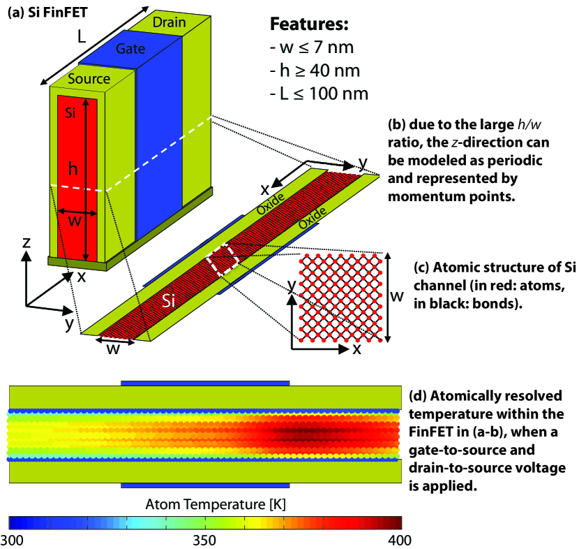
Figure 1. Schematic view of a 3-D Silicon FinFET.

1. Introduction

Heat dissipation in microchips reached alarming peak values of 100 W/cm² already in 2006 (wei; pop). This led to the end of Dennard scaling and the beginning of the “multicore crisis”, an era with energy-efficient parallel, but sequentially slower multicore CPUs. Now, more than ten years later, average power densities of up to 30 W/cm², about four times more than hot plates, are commonplace in modern high-performance CPUs, putting thermal management at the center of attention of circuit designers (hotplate). By scaling the dimensions of transistors more rapidly than their supply voltage, the semiconductor industry has kept increasing heat dissipation from one generation of microprocessors to the other. In this context, large-scale data and supercomputing centers are facing critical challenges regarding the design and cost of their cooling infrastructures. The price to pay for that has become exorbitant, as the cooling can be up to 40% of the total electicity consumed by data centers; a cumulative cost of many billion dollars per year.

Landauer’s theoretical limit of energy consumption for non-reversible computing offers a glimmer of hope: today’s processing units require orders of magnitude more energy than the $k_{B}T\ln 2$ Joule bound to (irreversibly) change one single bit. However, to approach this limit, it will be necessary to first properly understand the mechanisms behind nanoscale heat dissipation in semiconductor devices (pop). Fin field-effect transistors (FinFETs), as schematized in Fig. 1(a-c), build the core of all recent integrated circuits (ICs). Their dimensions do not exceed 100 nanometers along all directions, even 10 nm along one of them, with an active region composed of fewer than 1 million atoms. This makes them subject to strong quantum mechanical and peculiar thermal effects.

When a voltage is applied across FinFETs, electrons start to flow from the source to the drain contact, giving rise to an electrical current whose magnitude depends on the gate bias. The potential difference between source and drain allows electrons to transfer part of their energy to the crystal lattice surrounding them. This energy is converted into atomic vibrations, called phonons, that can propagate throughout FinFETs. The more atoms vibrate, the “hotter” a device becomes. This phenomenon, known as self- or Joule-heating, plays a detrimental role in today’s transistor technologies and has consequences up to the system level. It is illustrated in Fig. 1(d): a strong increase of the lattice temperature can be observed close to the drain contact of the simulated FinFET. The negative influence of self-heating on the CPU/GPU performance can be minimized by devising computer-assisted strategies to efficiently evacuate the generated heat from the active region of transistors.

Electro-thermal properties of nano-devices can be modeled and analyzed via Quantum Transport (QT) simulation, where electron and phonon currents are evaluated by taking quantum mechanics into account. Due to the large height/width ratio of FinFETs, these effects can be physically captured in a two-dimensional simulation domain comprising 10,000 to 15,000 thousand atoms. Such dissipative simulations involve solving the Schrödinger equation with open boundary conditions over several momentum and energy vectors that are coupled to each other through electron-phonon interactions. A straightforward algorithm to address this numerical problem consists of defining two loops, one over the momentum points and another one over the electron energies, which results in potentially extraneous execution dependencies and a complex communication pattern. The latter scales sub-optimally with the number of participating atoms and computational resources, thus limiting current simulations to the order of thousand atoms.

While the schedule (ordering) of the loops in the solver is natural from the physics perspective (§ 2), the data decomposition it imposes when parallelizing is not scalable from the computational perspective. To investigate larger device structures, it is crucial to reformulate the problem as a communication-avoiding algorithm — rescheduling computations across compute resources to minimize data movement.

Even when each node is operating at maximum efficiency, large-scale QT simulations are both bound by communication volume and memory requirements. The former inhibits strong scaling, as simulation time includes nanostructure-dependent point-to-point communication patterns, which becomes infeasible when increasing node count. The memory bottleneck is a direct result of the former. It hinders large simulations due to the increased memory requirements w.r.t. atom count. Transforming the QT simulation algorithm to minimize communication is thus the key to simultaneously model larger devices and increase scalability on different supercomputers.

The current landscape of supercomputing resources is dominated by heterogeneous nodes, where no two clusters are the same. Each setup requires careful tuning of application performance, focused mostly around data locality (padal). As this kind of tuning demands in-depth knowledge of the hardware, it is typically performed by a  Performance Engineer, a developer who is versed in intricate system details, existing high-performance libraries, and capable of modeling performance and setting up optimized procedures independently. This role, which complements the  Domain Scientist, has been increasingly important in scientific computing for the past three decades, but is now essential for any application beyond straightforward linear algebra to operate at extreme scales. Until recently, both Domain Scientists and Performance Engineers would work with one code-base. This creates a co-dependent  situation (pat-maccormicks-sos-talk), where the original domain code is tuned to a point that making modifications to the algorithm or transforming its behavior is difficult to one without the presence of the other, even if data locality or computational semantics are not changed.

In this paper, we propose a paradigm change by rewriting the problem from a data-centric perspective. We use OMEN, the current state-of-the-art quantum transport simulation application (omen), as our baseline, and show that the key to formulating a communication-avoiding variant is tightly coupled with recovering local and global data dependencies of the application. We start from a reference Python implementation, using Data-Centric (DaCe) Parallel Programming (sdfg) to express the computations separately from data movement. DaCe automatically constructs a stateful dataflow view that can be used to optimize data movement without modifying the original computation. This enables rethinking the communication pattern of the simulation, and tuning the data movement for each target supercomputer.

In sum, the paper makes the following contributions:

• Construction of the dissipative quantum transport simulation problem from a physical perspective;

• Definition of the stateful dataflow of the algorithm, making data and control dependencies explicit on all levels;

• Creation of a novel tensor-free communication-avoiding variant of the algorithm based on the data-centric view;

• Optimal choice of the decomposition parameters based on the modeling of the performance and communication of our variant, nano-device configuration, and cluster architecture;

• Demonstration of the algorithm’s scalability on two vastly different supercomputers — Piz Daint and Summit — up to full-scale runs on 10k atoms, 21 momentum points and 1,000 energies per momentum;

• A performance increase of 1–2 orders of magnitude over the previous state of the art, all from a data-centric Python implementation that reduces code-length by a factor of five.

2. Statement of the Problem

A technology computer aided design (TCAD) tool can shed light on the electro-thermal properties of nano-devices, provided that it includes the proper physical models:

• The dimensions of FinFETs calls for an atomistic quantum mechanical treatment of the device structures;

• The electron and phonon bandstructures should be accurately and fully described;

• The interactions between electrons and phonons, especially energy exchanges, should be accounted for.

The Non-equilibrium Green’s Function (NEGF) formalism (datta) combined with density functional theory (DFT) (kohn) fulfills all these requirements and lends itself optimally to the investigation of self-heating in arbitrary device geometries. With NEGF, both electron and phonon transport can be described, together with their respective interactions. With the help of DFT, an ab initio method, any material (combination) can be handled at the atomic level without the need for empirical parameters.

FinFETs are essentially three-dimensional (3-D) components that can be approximated as 2-D slices in the $x$-$y$ plane, whereas the height, aligned with the $z$-axis (see Fig. 1(a-b)), can be treated as a periodic dimension and represented by a momentum vector $k_{z}$ or $q_{z}$ in the range $[-\pi,\pi]$. Hence, the DFT+NEGF equations have the following form:

(3) $$\left\{\begin{array}[]{l}\left(E\cdot{\mathbf{S}}(k_{z})-{\mathbf{H}}(k_{z})-{\mathbf{\Sigma}}^{R}(E,k_{z})\right)\cdot{\mathbf{G}}^{R}(E,k_{z})={\mathbf{I}}\\ {\mathbf{G}}^{\gtrless}(E,k_{z})=\mathbf{G}^{R}(E,k_{z})\cdot{\mathbf{\Sigma}}^{\gtrless}(E,k_{z})\cdot{\mathbf{G}}^{A}(E,k_{z}).\end{array}\right.$$

In Eq. (3), $E$ is the electron energy, ${\mathbf{S}}(k_{z})$ and ${\mathbf{H}}(k_{z})$ the overlap and Hamiltonian matrices, respectively. They typically exhibit a block tri-diagonal structure and a size $N_{A}\times N_{orb}$ with $N_{A}$ as the total number of atoms in the considered structure and $N_{orb}$ the number of orbitals (basis components) representing each atom. The ${\mathbf{S}}(k_{z})$ and ${\mathbf{H}}(k_{z})$ matrices must be produced by a DFT package relying on a localized basis set, e.g., SIESTA (siesta) or CP2K (cp2k). The ${\mathbf{G}}(E,k_{z})$’s refer to the electron Green’s Functions (GF) at energy $E$ and momentum $k_{z}$. They are of the same size as ${\mathbf{S}}(k_{z})$, ${\mathbf{H}}(k_{z})$, and ${\mathbf{I}}$, the identity matrix. The GF can be either retarded ($R$), advanced ($A$), lesser ($<$), or greater ($>$) with ${\mathbf{G}}^{A}(E,k_{z})$=$\left({\mathbf{G}}^{R}(E,k_{z})\right)^{T}$. The same conventions apply to the self-energies ${\mathbf{\Sigma}}(E,k_{z})$ that include a boundary and a scattering term. The former connects the simulation domain to external contacts, whereas the latter encompasses all possible interactions of electrons with their environment.

To handle phonon transport, the following NEGF-based system of equations must be processed:

(6) $$\left\{\begin{array}[]{l}\left(\omega^{2}\cdot{\mathbf{I}}-{\mathbf{\Phi}}(q_{z})-{\mathbf{\Pi}}^{R}(\omega,q_{z})\right)\cdot{\mathbf{D}}^{R}(\omega,q_{z})={\mathbf{I}}\\ {\mathbf{D}}^{\gtrless}(\omega,q_{z})={\mathbf{D}}^{R}(\omega,q_{z})\cdot{\mathbf{\Pi}}^{\gtrless}(\omega,q_{z})\cdot{\mathbf{D}}^{A}(\omega,q_{z}),\end{array}\right.$$

where the ${\mathbf{D}}(\omega,q_{z})$’s are the phonon Green’s functions at frequency $\omega$ and momentum $q_{z}$ and the ${\mathbf{\Pi}}(\omega,q_{z})$’s the self-energies, while ${\mathbf{\Phi}}(q_{z})$ refers to the dynamical (Hessian) matrix of the studied domain, computed with density functional perturbation theory (DFPT) (dfpt). The phonon Green’s Function types are the same as for electrons (retarded, advanced, lesser, and greater). All matrices involved in Eq. (6) are of size $N_{A}\times N_{3D}$, $N_{3D}$=3 corresponding to the number of directions along which the crystal can vibrate ($x$, $y$, $z$).

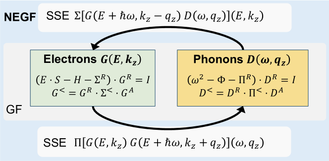
Figure 2. Self-consistent coupling between the GF and SSE phases (kernels) as part of the NEGF formalism.

Equations (3) and (6) must be solved for all possible electron energy ($N_{E}$) and momentum ($N_{k_{z}}$) points as well as all phonon frequencies ($N_{\omega}$) and momentum ($N_{q_{z}}$). This can be done with a so-called recursive Green’s Function (RGF) algorithm (rgf) that takes advantage of the block tri-diagonal structure of the matrices ${\mathbf{H}}$, ${\mathbf{S}}$, and ${\mathbf{\Phi}}$. All matrices can be divided into $bnum$ blocks with $\frac{N_{A}}{bnum}$ atoms each, if the structure is homogeneous, as here. RGF then performs a forward and backward pass over the $bnum$ blocks that compose the 2-D slice. Both passes involve a number of multiplications between matrices of size $\left(\frac{N_{A}}{bnum}N_{orb}\right)^{2}$ for electrons (or $\left(\frac{N_{A}}{bnum}N_{3D}\right)^{2}$ for phonons) for each block.

The main computational bottleneck does not come from RGF, but from the fact that in the case of self-heating simulations the energy-momentum ($E$,$k_{z}$) and frequency-momentum ($\omega$,$q_{z}$) pairs are not independent from each other, but tightly coupled through the scattering self-energies (SSE) ${\mathbf{\Sigma}}^{R\gtrless,S}$ and ${\mathbf{\Pi}}^{R\gtrless,S}$. These matrices are made of blocks of size $N_{orb}\times N_{orb}$ and $N_{3D}\times N_{3D}$, respectively, and are given by (stieger):

$${\mathbf{\Sigma}}^{\gtrless S}_{aa}(E,k_{z})=i\sum_{q_{z}ijl}\int\frac{d\hbar\omega}{2\pi}\left[\nabla_{i}{\mathbf{H}}_{ab}\cdot{\mathbf{G}}^{\gtrless}_{bb}(E-\hbar\omega,k_{z}-q_{z})\cdot\right.$$

$$\nabla_{j}{\mathbf{H}}_{ba}\cdot\left({\mathbf{D}}^{\gtrless ij}_{ba}(\omega,q_{z})-{\mathbf{D}}^{\gtrless ij}_{bb}(\omega,q_{z})-\right.$$

(7) $$\left.\left.{\mathbf{D}}^{\gtrless ij}_{aa}(\omega,q_{z})+{\mathbf{D}}^{\gtrless ij}_{ab}(\omega,q_{z})\right)\right],$$

(8) $${\mathbf{\Pi}}^{\gtrless S}_{aa}(\omega,q_{z})=-i\sum_{k_{z}l}\int\frac{dE}{2\pi}\mathrm{tr}\left\{\nabla_{i}{\mathbf{H}}_{ba}\cdot{\mathbf{G}}^{\gtrless}_{aa}(E+\hbar\omega,k_{z}+q_{z})\cdot\right.$$

$$\left.\nabla_{j}{\mathbf{H}}_{ab}\cdot{\mathbf{G}}^{\lessgtr}_{bb}(E,k_{z})\right\},$$

(9) $${\mathbf{\Pi}}^{\gtrless S}_{ab}(\omega,q_{z})=i\sum_{k_{z}}\int\frac{dE}{2\pi}\mathrm{tr}\left\{\nabla_{i}\mathbf{H}_{ba}\cdot\mathbf{G}^{\gtrless}_{aa}(E+\hbar\omega,k_{z}+q_{z})\cdot\right.$$

$$\left.\nabla_{j}\mathbf{H}_{ab}\cdot\mathbf{G}^{\lessgtr}_{bb}(E,k_{z})\right\}.$$

In Eqs. (7-9), all Green’s Functions ${\mathbf{G}_{ab}}$ (${\mathbf{D}_{ab}}$) are matrices of size $N_{orb}\times N_{orb}$ ($N_{3D}\times N_{3D}$). They describe the coupling between all orbitals (vibrational directions) of two neighbor atoms $a$ and $b$ situated at position ${\mathbf{R}}_{a}$ and ${\mathbf{R}}_{b}$. Each atom possesses $N_{B}$ neighbors. Furthermore, $\nabla_{i}{\mathbf{H}}_{ab}$ is the derivative of the Hamiltonian block $\mathbf{H}_{ab}$ coupling atoms $a$ and $b$ w.r.t variations along the $i$=$x$, $y$, or $z$ coordinate of the bond $\mathbf{R}_{b}-\mathbf{R}_{a}$. To obtain the retarded components of the scattering self-energies, the following relationship can be used: ${\mathbf{\Sigma}}^{R}\approx({\mathbf{\Sigma}}^{>}-{\mathbf{\Sigma}}^{<})/2$, which is also valid for ${\mathbf{\Pi}}^{R}$(lake). Due to computational reasons, only the diagonal blocks of ${\mathbf{\Sigma}}^{R\gtrless,S}$ are retained, while $N_{B}$ non-diagonal connections are kept for ${\mathbf{\Pi}}^{R\gtrless,S}$.

Table 1. Typical QT Simulation Parameters

Variable	Description	Range
$N_{k_{z}}$	Number of electron momentum points	$[1,21]$
$N_{q_{z}}$	Number of phonon momentum points	$[1,21]$
$N_{E}$	Number of energy points	[700, 1500]
$N_{\omega}$	Number of phonon frequencies	[10, 100]
$N_{A}$	Total number of atoms per device structure	See Table  2
$N_{B}$	Neighbors considered for each atom	[4, 50]
$N_{orb}$	Number of orbitals per atom	[1, 30]
$N_{3D}$	Degrees of freedom for crystal vibrations	3

Table 2. State of the Art Quantum Transport Simulators

Name	Maximum # of Computed Atoms						Scalability
	Tight-binding-like∗			DFT			Max. Cores	Using
	$GF^{\dagger}_{e}$	$GF^{\dagger}_{ph}$	$GF+SSE$	$GF^{\dagger}_{e}$	$GF^{\dagger}_{ph}$	$GF+SSE$	(Magnitude)	GPUs
GOLLUM (ferrer2014gollum)	1k	1k	—	100	100	—	N/A	✗
Kwant (groth2014kwant)	10k	—	—	—	—	—	N/A	✗
NanoTCAD ViDES (vides)	10k	—	—	—	—	—	N/A	✗
QuantumATK (atk)	10k	10k	—	1k	1k	—	1k	✗
TB_sim (niquet)	100k	—	10k‡	1k	—	—	10k	✓
NEMO5 (nemo5)	100k	100k	10k‡	—	—	—	100k	✓
OMEN (omen)	100k (1.44 Pflop/s (sc11))	100k	10k	10k	10k (15 Pflop/s (sc15))	1k (0.16 Pflop/s)	100k	✓
This work	N/A	N/A	N/A	10k	10k	10k (19.71 Pflop/s)	1M	✓

^∗: including Maximally-Localized Wannier Functions (MLWF), $\dagger$: Ballistic, $\ddagger$: Simplified.

The evaluation of Eqs. (7-9) does not require the knowledge of all entries of the ${\mathbf{G}}$ and ${\mathbf{D}}$ matrices, but of two (lesser and greater) 5-D tensors of shape $[N_{k_{z}},N_{E},N_{A},N_{orb},N_{orb}]$ for electrons and two 6-D tensors of shape $[N_{q_{z}},N_{\omega},N_{A},N_{B}+1,N_{3D},N_{3D}]$ for phonons. Each $[k_{z},E,N_{A},N_{orb},N_{orb}]$ and $[q_{z},\omega,N_{A},N_{B}+1,N_{3D},$ $N_{3D}]$ combination is produced independently from the other by solving Eq. (3) and (6), respectively. The electron and phonon scattering self-energies can also be reshaped into multi-dimensional tensors that have exactly the same dimensions as their Green’s functions counterparts. However, the self-energies cannot be computed independently, one energy-momentum or frequency-momentum pair depending on many others, as defined in Eqs. (7-9) and depicted in Fig. 2. Furthermore, ${\mathbf{\Sigma}}^{\gtrless S}(E,k_{z})$ is a function of ${\mathbf{D}}^{\gtrless}(\omega,q_{z})$, while ${\mathbf{G}}^{\gtrless S}(E,k_{z})$ is needed to calculate ${\mathbf{\Pi}}^{\gtrless}(\omega,q_{z})$.

To obtain the electrical and energy currents that flow through a given device and the corresponding charge density, Eqs. (3-6) (GF) and Eqs. (7-9) (SSE) must be iteratively solved until convergence is reached, and all GF contributions must be accumulated (stieger). The algorithm starts by setting ${\mathbf{\Sigma}}^{\gtrless}(E,k_{z})$=${\mathbf{\Pi}}^{\gtrless}(\omega,q_{z})$=0 and continues by computing all GFs under this condition. The latter then serve as inputs to the next phase, where the SSE are evaluated for all ($k_{z}$,$E$) and ($q_{z}$,$\omega$) pairs. Subsequently, the SSE matrices are fed into the GF calculation and the process repeats itself until the GF variations do not exceed a pre-defined threshold. In terms of HPC, the main challenges reside in the distribution of these quantities over thousands of compute units, the resulting communication-intensive gathering of all data to handle the SSE phase, and the efficient solution of Eqs. (7-9) on hybrid nodes, as they involve many small matrix multiplications. Typical simulation parameters are listed in Table 1.

2.1. Current State of the Art

There exist several atomistic quantum transport simulators (ferrer2014gollum; groth2014kwant; nemo5; atk; vides; niquet; omen) that can model the characteristics of nano-devices. Their performance is summarized in Table 2, where their estimated maximum number of atoms that can be simulated for a given physical model is provided. Only orders of magnitude are shown, as these quantities depend on the device geometries and bandstructure method. It should be mentioned that most tools are limited to tight-binding-like (TB) Hamiltonians, because they are computationally cheaper than DFT ones ($N_{orb,TB}<N_{orb,DFT}$ and $N_{B,TB}\ll N_{B,DFT}$). This explains the larger systems that can be treated with TB. However, such approaches lack accuracy when it comes to the exploration of material stacks, amorphous layers, metallic contacts, or interfaces. In these cases, only DFT ensures reliable results, but at much higher computational cost.

To the best of our knowledge, the only tool that can solve Eqs. (3) to (9) self-consistently, in structures composed of thousands of atoms, at the DFT level is OMEN, a two times Gordon Bell Prize finalist (sc11; sc15). The code is written in C++, contains 90,000 lines of code in total, and uses MPI as its communication protocol. Some parts of it have been ported to GPUs using the CUDA language and taking advantage of libraries such as cuBLAS, cuSPARSE, and MAGMA. The electron-phonon scattering model was first implemented based on the tight-binding method and a three-level MPI distribution of the workload (momentum, energy, and spatial domain decomposition). A first release of the model with equilibrium phonon (${\mathbf{\Pi}}$=0) was validated up to 95k cores for a device with $N_{A}$=5,402, $N_{B}$=4, $N_{orb}$=10, $N_{k_{z}}$=21, and $N_{E}$=1,130. These runs showed that the application can reach a parallel efficiency of 57%, when going from 3,276 up to 95,256 cores, with the SSE phase consuming from 25% to 50% of the total simulation times. The reason for the SSE increase could be attributed to the communication time required to gather all Green’s Function inputs for Eq. (7), which grew from 16 to 48% of the total simulation time (sc10) as the number of cores went from 3,276 to 95,256.

After extending the electron-phonon scattering model to DFT and adding phonon transport to it, it has been observed that the time spent in the SSE phase (communication and computation) explodes. Even for a small structure with $N_{A}$=2,112, $N_{orb}$=4, $N_{k_{z}}$=$N_{q_{z}}$=11, $N_{E}$=650, $N_{\omega}$=30, and $N_{B}$=13, 95% of the total simulation time is dedicated to SSE, regardless of the number of used cores/nodes, among which $\sim$60% for the communication between the different MPI tasks. To simulate self-heating in realistic FinFETs ($N_{A}>$10,000), with a high accuracy ($N_{k_{Z}}>$20, $N_{E}>$1,000), and within reasonable times (a couple of minutes for one GF-SSE iteration at machine scale), the algorithms involved in the solution of Eqs. (3) to (9) must be drastically improved: as compared to the state of the art, an improvement of at least one order of magnitude is needed in terms of the number of atoms that can be handled, and two orders of magnitude for what concerns the computational time.

3. Data-Centric Parallel Programming

Communication-Avoiding (CA) algorithms (demmel13ca; writeav) are defined as algorithm variants and schedules (orders of operations) that minimize the total number of performed memory loads and stores, achieving lower bounds in some cases. To achieve such bounds, a subset of those algorithms is matrix-free, potentially reducing communication at the expense of recomputing parts of the data on-the-fly. A key requirement in modifying an algorithm to achieve communication avoidance is to explicitly formulate its data movement characteristics. The schedule can then be changed by reorganizing the data flow to minimize the sum of accesses in the algorithm. Recovering a Data-Centric (DaCe) view of an algorithm, which makes movement explicit throughout all levels (from a single core to the entire cluster), is thus the path forward in scaling up the creation of CA variants to more complex algorithms and multi-level memory hierarchies as one.

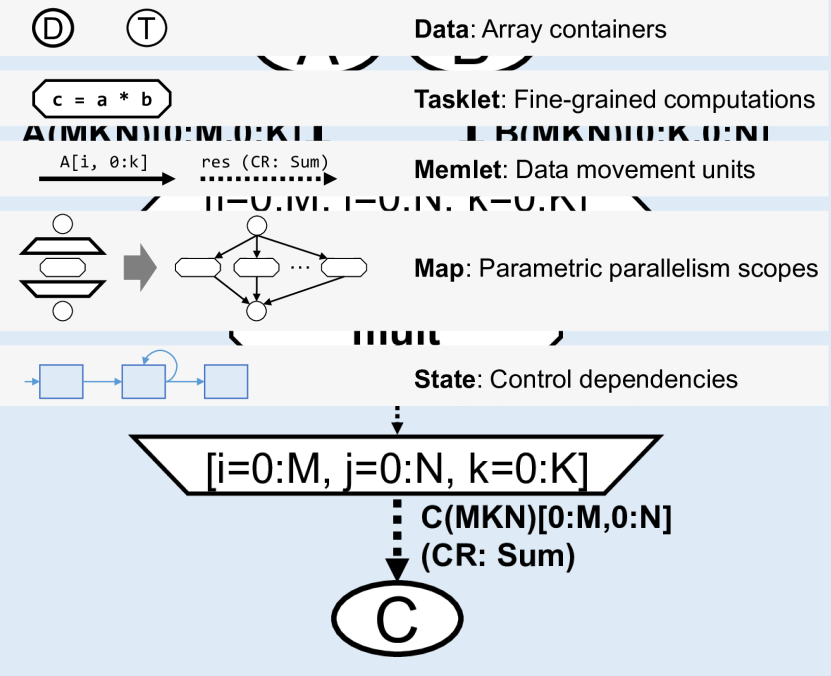
Figure 3. SDFG concepts and syntax.

DaCe defines a development workflow where the original algorithm is independent from its data movement representation, enabling symbolic analysis and transformation of the latter without modifying the scientific code. This way, a CA variant can be formulated and developed by a performance engineer, while the original algorithm retains readability and maintainability. At the core of the DaCe implementation is the Stateful DataFlow multiGraph (SDFG) (sdfg), an intermediate representation that encapsulates data movement and can be generated from high-level code in Python. The syntax (node and edge types) of SDFGs is listed in Fig. 3. The workflow is as follows: The domain scientist designs an algorithm and implements it as linear algebra operations (imposing dataflow implicitly), or using Memlets and Tasklets (specifying dataflow explicitly). This implementation is then parsed into an SDFG, where performance engineers may apply graph transformations to improve data locality. After transformation, the optimized SDFG is compiled to machine code for performance evaluation. It may be further transformed interactively and tuned for different target platforms and memory hierarchy characteristics.

Figure 4. Matrix multiplication in DaCe.

An example of a naïve matrix multiplication SDFG (C = A @ B in Python) is shown in Fig. 4. In the figure, we see that data flows from Data nodes A and B through a Map scope. This would theoretically expand to M*N*K multiplication Tasklets (mult), where the contribution of each Tasklet (i.e., a multiplied pair) will be summed in Data node C (due to conflicting writes that are resolved by CR: Sum). The Memlet edges define all data movement, which is seen in the input and output of each Tasklet, but also entering and leaving the Map with its overall requirements (in brackets) and number of accesses (in parentheses). The accesses and ranges are symbolic expressions, which can be summed to obtain the algorithm’s data movement characteristics. The SDFG representation allows the performance engineer to add transient (local) arrays, reshape and nest Maps (e.g., to impose a tiled schedule), fuse multiple scopes, map computations to accelerators (GPUs and FPGAs), and other transformations that may modify the overall number of accesses.

⬇

1# Declaration of symbolic variables

2Nkz, NE, Nqz, Nw, N3D, NA, NB, Norb = (

3 dace.symbol(name)

4 for name in [’Nkz’, ’NE’, ’Nqz’, ’Nw’,

5 ’N3D’, ’NA’, ’NB’, ’Norb’])

6

7@dace.program

8def sse_sigma(neigh_idx: dace.int32[NA, NB],

9 dH: dace.float64[NA, NB, N3D, Norb, Norb],

10 G: dace.complex128[Nkz, NE, NA, Norb, Norb],

11 D: dace.complex128[Nqz, Nw, NA, NB, N3D, N3D],

12 Sigma: dace.complex128[Nkz, NE, NA, Norb, Norb]):

13

14 # Declaration of Map scope

15 for k, E, q, w, i, j, a, b in dace.map[0:Nkz, 0:NE,

16 0:Nqz, 0:Nw,

17 0:N3D, 0:N3D,

18 0:NA, 0:NB]:

19 f = neigh_idx[a, b]

20 dHG = G[k-q, E-w, f] @ dH[a, b, i]

21 dHD = dH[a, b, j] * D[q, w, a, b, i, j]

22 Sigma[k, E, a] += dHG @ dHD

23

24if __name__ == ’__main__’:

25 # Initialize symbolic variables

26 Nkz.set(21)

27 NE.set(1000)

28 ...

29 # Initialize input/output arrays

30 idx = numpy.ndarray((NA.get(), NB.get()), numpy.int32)

31 ...

32 # Call dace program

33 sse_sigma(neigh_idx=idx, dH=dH, G=G, D=D, Sigma=Sigma)\end{lstlisting}

34 \vspace{-1em}

35 \caption{$\Sigma^\gtrless$ computation in Python}

36 \vspace{-1em}

37 \label{fig:frontend}

38\end{figure}

39

40Fig.~\ref{fig:frontend} \hl{shows the computation of $\Sigma^\gtrless$ in DaCe, implemented

41with linear algebra operations in a Python-based frontend, while the resulting SDFG is presented in} Fig.~\ref{fig:sse-initial}.

42\hl{Symbolic variables, such as the number of atoms, momentums and energies, are

43declared in lines 2-5.}

44\hl{The \texttt{dace.program} decorator (line 7) is used to define the function to be converted to an SDFG.

45Type annotations in the function signature (lines 8-12) are used to define the datatype

46and shape of the input and output arrays.}

47\hl{For-loop statements using the \texttt{dace.map} iterator (lines 15-18) define a Map scope.

48Linear algebra operations (lines 20-22) are automatically parsed to Tasklets.

49The latter can be subsequently lowered to nested SDFGs that implement

50these operations in fine-grained dataflow, such as the matrix multiplication SDFG

51in} Fig.~\ref{fig:dacemm}. \hl{Alternatively, they can be mapped to optimized BLAS calls

52when generating code.

53The DaCe program is executed through Python host code (lines 24-33), where the

54symbolic variables, input and output arrays are initialized.}

55

56

57Our main innovation in optimizing the OMEN QT simulator lies in

58the use of the DaCe parallel programming framework.

59In the following section, we show how the data-centric view provided by DaCe

60is used to identify and implement a \textit{tensor-free} CA variant of OMEN,

61achieving optimal communication for the first time

62in this scientific domain.

63

64

65

66\section{Transforming OMEN}

67

68To understand the dataflow of the OMEN implementation, its 90,000 lines of code, or 15,798 lines\footnote{generated using David A. Wheeler’s ’SLOCCount’.} of core RGF and SSE computations can be examined.

69Alternatively, the SDFG could be used to obtain a hierarchical view of the application, where States and Map scopes can be collapsed.

70A deeper dive allows optimization of certain regions.

71Below, we take a methodological top-down approach to transform the OMEN SDFG,

72starting from its high-level decomposition, which generates the communication,

73through individual computational kernels, to small-scale linear algebra operations.

74We instrument the code in order to find bottlenecks and critical subgraphs to ‘‘cut out’’ and transform.

75Furthermore, we support our decisions with communication and performance models obtained using

76the data-centric representation.

77

78\begin{figure}[b]

79 \centering

80 \includegraphics[width=\linewidth, page=2]{figures/omen_figures.pdf}

81 \vspace{-2em}

82 \caption{SDFG of QT simulation: high-level performance engineer view of the problem.}

83 \label{fig:dace-view}

84\end{figure}

85

86

87

88The top-level view of the QT simulation algorithm can be seen in Fig.~\ref{fig:dace-view}.

89The SDFG shows that the simulation iterates over two states, GF and SSE.

90The former computes the Green’s Functions, boundary conditions, and the electrical current. The state consists of two concurrent Maps, one for the electrons and one for the phonons (\S~\ref{sec:problem}).

91The SSE state computes the scattering Self-Energies ${\mathbf \Sigma}^\gtrless$ and ${\mathbf \Pi}^\gtrless$.

92At this point, we opt to represent the RGF solvers and SSE kernel as Tasklets, i.e., collapsing their dataflow, so as to focus on high-level aspects of the algorithm. %, because they operate on all the atoms for a specific energy-momentum pair.

93This view indicates that the RGF solver cannot compute the Green’s Functions for a specific atom separately from the rest of the material (operating on all atoms for a specific energy-momentum pair), and that SSE

94outputs the contribution of a specific

95$\left(k_z, E, q_z, \omega, a, b\right)$ point to ${\mathbf \Sigma}^\gtrless$ and ${\mathbf \Pi}^\gtrless$.

96These contributions are then accumulated to the output tensors, as indicated by the dotted Memlet edges.

97The accumulation is considered associative; therefore the map can compute all dimensions of the inputs and outputs in parallel.

98

99

100

101\subsection{Communication Avoidance}\label{sec:ca}

102

103\begin{figure}[t]

104 \centering

105 \includegraphics[width=\linewidth, page=14]{figures/omen_figures.pdf}

106 \vspace{-1em}

107 \caption{Map-tiling SSE (left) and resulting Memlets (right).}

108 \vspace{-1em}

109 \label{fig:ssetiling}

110 % \end{subfigure}\qquad

111 % \begin{subfigure}[b]{.45\linewidth}

112 % \centering

113 % \includegraphics[height=1.6in, page=19]{figures/omen_figures_2.pdf}

114 % \caption{Memlet propagation for one of the ${\mathbf G}^\gtrless$ accesses.}

115 % \label{fig:sse-prop}

116 % \end{subfigure}

117 % \vspace{-1em}

118 % \caption{High-level SSE transformation.}

119 % \vspace{-1em}

120 % \label{fig:sse-hl}

121\end{figure}

122

123The applications shown in Table~\ref{tab:competitors}, including OMEN, have been developed mainly by domain scientists, and thus use the ‘‘natural’’ decomposition construction of momentum points and energies, as shown in Fig.~\ref{fig:dace-view}.

124As a result, the communication scheme for SSE in OMEN is split to $N_{q_z}N_{\omega}$ rounds.

125In each round:

126\begin{itemize}

127\item The phonon Green’s Functions ${\mathbf D}^\gtrless(\omega, q_z)$ are broadcast to all processes;

128\item Each process iterates over its assigned electron Green’s Functions ${\mathbf G}^\gtrless(E, k_z)$,

129and sends the corresponding ${\mathbf G}^\gtrless(E\pm\hbar\omega, k_z+q_z)$ to the processes that need them;

130\item Each process iterates over its assigned electron Green’s Functions ${\mathbf G}^\gtrless(E, k_z)$

131and receives the corresponding ${\mathbf G}^\gtrless(E\pm\hbar\omega, k_z-q_z)$;

132\item The partial phonon self-energies $\Pi_p^\gtrless(\omega, q_z)$ produced by each process are reduced

133to ${\mathbf \Pi}^\gtrless(\omega, q_z)$.

134\end{itemize}

135Based on the above, we make the following observations:

136\begin{itemize}

137\item The full 6-D tensors ${\mathbf D}^\gtrless$ are broadcast to all processes;

138\item The full 5-D tensors ${\mathbf G}^\gtrless$ are replicated through point-to-point communication $2N_{q_z}N_{\omega}$ times.

139\end{itemize}

140We use DaCe to transform the SSE state and find optimal data distributions and communication schemes in the following manner:

141First, we tile the SSE map (Fig.~\ref{fig:ssetiling} left, differences highlighted in bold) across all dimensions,

142with the intention of assigning each tile to a different process.

143The tiling graph transformation splits a map to two nested ones, where each dimension

144of the original map is partitioned to $n_d$ approximately equal ranges of size $s_d$.

145For example, the electron momentum dimension is partitioned to $n_{k_z}$ ranges of size $s_{k_z}$ each. The corresponding symbol $t_{k_z}$ in the outer map spans the partitions, whereas the inner symbol $k_z$ takes values in the range $\left[t_{k_z}s_{k_z}, \left(t_{k_z}+1\right)s_{k_z}\right)$.

146Likewise, $q_z$ iterates over $\left[t_{q_z}s_{q_z}, \left(t_{q_z}+1\right)s_{q_z}\right)$.

147

148

149Subsequently, the DaCe framework propagates the data access expressions in Memlets from the Tasklets outwards, through scopes.

150DaCe automatically computes contiguous and strided ranges, but can only over-approximate some irregular accesses. In these cases, performance engineers can manually provide

151the additional information to the SDFG, creating new optimization opportunities.

152

153In particular, the propagation of the access ${\mathbf G}^\gtrless[k_z-q_z,E-\omega,f(a,b)]$

154is shown in Fig.~\ref{fig:ssetiling} (right).

155The propagated range of the index expression $k_z-q_z$ is computed automatically as

156$[t_{k_z}s_{k_z}-\left(t_{q_z}+1\right)s_{q_z}+1,$ $\left(t_{k_z}+1\right)s_{k_z}-t_{q_z}s_{q_z})$.

157The total number of accesses over this range is $s_{k_z}+s_{q_z}-1$, while the length,

158which coincides with the number of unique accesses,

159is $\min\left(N_{k_z}, s_{k_z}+s_{q_z}-1\right)$.

160However, the expression $f(a,b)$, which represents the index of the $b$-th neighbor of atom $a$, %, which is in the range $\left[0,N_A\right)$.

161is an indirection through a matrix of the atom couplings.

162DaCe cannot propagate such indices and thus the performance engineer must provide a model or expression manually.

163

164For this work, we do not to tile the dimensions of the atom neighbors.

165Instead, we make use of the observation that atoms with neighboring indices are

166very often neighbors in the coupling matrix.

167A good approximation to the propagation of $f(a,b)$ over the range

168$\left[t_as_a, \left(t_a+1\right)s_a\right)\times\left[0, N_B\right)$ is then

169$\big[\min\left(0, t_as_a-\frac{N_B}{2}\right),\allowbreak\max\left(N_A, \left(t_a+1\right)s_a+\frac{N_B}{2}\right)\big)$.

170The total number of accesses incr-eases to $s_aN_B$, while the length of this range is

171$\min\left(N_A, s_a + N_B\right)$.

172

173After Memlet propagation is complete, the total length of the Memlet ranges between the

174two maps provides the amount of data that each process must

175load/store or communicate over the network.

176An \textit{\textbf{optimal communication scheme}} can subsequently be found by minimizing these expressions.

177For this work, we perform exhaustive search over the feasible tile sizes.

178Since the combinations of the latter are in the order of $10^6$ for most simulation parameters and number of processes,

179the search completes in just a few seconds.

180

181We demonstrate the power of the above approach by comparing the OMEN communication

182scheme against partitioning the atom and electron-energy dimensions.

183Using the original OMEN data distribution, each process:

184\begin{itemize}

185\item receives $64\frac{N_{k_z}N_E}{P}N_{q_z}N_{\omega}N_AN_{orb}^2$ bytes for the electron\\ Green’s Functions ${\mathbf G}^\gtrless$;

186\item sends and receives a total of $64N_{q_z}N_{\omega}N_AN_BN_{3D}^2$ bytes for the phonon Green’s functions ${\mathbf D}^\gtrless$ and self-energies ${\mathbf \Pi}^\gtrless$;

187\end{itemize}

188where $P$ is the number of processes.

189The DaCe-transformed SDFG changes the distribution of the data between the GF

190and SSE states, which yields all-to-all collective operations (\texttt{alltoallv} in the MPI standard). Specifically, each process contributes:

191\begin{itemize}

192\item $64N_{k_z}\left(\frac{N_E}{T_E}+2N_\omega\right)\left(\frac{N_A}{T_A}+N_B\right)N_{orb}^2$ bytes for the electron Green’s functions ${\mathbf G}^\gtrless$ and self-energies ${\mathbf \Sigma}^\gtrless$;

193\item $64N_{q_z}N_{\omega}\left(\frac{N_A}{T_A}+N_B\right)N_BN_{3D}^2$ bytes for ${\mathbf D}^\gtrless$ and ${\mathbf \Pi}^\gtrless$.

194\end{itemize}

195$T_E$ and $T_A$ are the number of partitions of the energies and atoms respectively, with $P = T_ET_A$.

196For ${\mathbf D}^\gtrless$ and ${\mathbf \Pi}^\gtrless$, the DaCe-based communication scheme reduces the factor

197$N_AN_B$ to $\frac{N_A}{T_A}+N_B$.

198In the case of ${\mathbf G}^\gtrless$, this scheme eliminates the quadratic factor over the number of momentum points exhibited by OMEN.

199

200

201

202

203

204

205\subsection{Dataflow Optimizations}\label{sec:dataflow}

206

207The data-centric view not only encompasses macro dataflow that imposes communication, but

208also data movement within compute devices. We use DaCe to transform all computations in

209the communication-avoiding variant of OMEN, including the RGF algorithm, SSE, and boundary

210conditions, and automatically generate GPU code. Below we cut-out and showcase a subset of these transformations, focusing on a

211bottleneck subgraph of the QT simulator, which is found within the SSE kernel: computing

212${\mathbf \Sigma}^\gtrless$ as in Eq.~(\ref{eq:3}). We note that computation of ${\mathbf \Pi}^\gtrless$ is

213transformed in a similar manner.

214

215\begin{figure}

216 \centering

217 \includegraphics[clip, height=2.4in, page=3]{figures/omen_figures.pdf}

218 \vspace{-1em}

219 \caption{Initial SDFG of ${\mathbf \Sigma}^\gtrless$ computation in SSE.}

220 \label{fig:sse-initial}

221\end{figure}

222

223Fig.~\ref{fig:sse-initial} gives the initial representation of the computation, generated from a reference Python implementation. The inputs are:

224\begin{itemize}

225\item $\mathbf{G}^\gtrless$: Electron Green’s Functions, a 3-D array of $N_{orb}^2$ matrices

226and size $N_{k_z} \times N_E \times N_A$;

227\item $\mathbf{\nabla {\mathbf H}}$: Derivative of the Hamiltonian, a 3-D array of $N_{orb}^2$ matrices

228and size $N_A \times N_B \times N_{3D}$;

229\item $\mathbf{D}^\gtrless$: Phonon Green’s Functions, a 6-D array of scalar values

230and size $N_{q_z} \times N_\omega \times N_A \times N_B \times N_{3D}^2$. Prior to the kernel, the Green’s Functions have been preprocessed to contain the values

231${\mathbf D}^{\gtrless ij}_{ln}(\omega,q_z)-{\mathbf D}^{\gtrless ij}_{ll}(\omega,q_z)-

232{\mathbf D}^{\gtrless ij}_{nn}(\omega,q_z)+{\mathbf D}^{\gtrless ij}_{nl}(\omega,q_z)$,

233as described in Eq.~(\ref{eq:3}).

234\end{itemize}

235The outputs are the electron self-energies ${\mathbf \Sigma}^\gtrless$, which are also a

2363-D array of $N_{orb}^2$ matrices with the same dimensions as ${\mathbf G}^\gtrless$.

237The SDFG consists of a map over the 8-D space

238$\left[0, N_{k_z}\right)\times\left[0, N_E\right)\times\left[0, N_{q_z}\right)\times

239\left[0, N_\omega\right)\times\left[0, N_{3D}\right)\times\left[0, N_{3D}\right)\times

240\left[0, N_A\right)\times\left[0, N_B\right)$. For each $\left(k_z,E,q_z,\omega,i,j,a,b\right)$ point

241in this space, the following computations must be performed:

242\begin{enumerate}

243\item The matrices at indices ${\mathbf G}^\gtrless[k_z-q_z,E-\omega,f]$ and $\nabla {\mathbf H}[a,b,i]$

244are multiplied (‘‘\texttt{@}’’ symbol) and the result is stored in the temporary matrix $\nabla {\mathbf H}{\mathbf G}^\gtrless$.

245The index $f$ in the array ${\mathbf G}^\gtrless$ is an indirection $f(a,b)$ in

246the space $\left[0, N_A\right)$;

247\item The matrix at index $\nabla {\mathbf H}[a,b,j]$ is multiplied by the scalar value

248${\mathbf D}^\gtrless[q_z,\omega,a,b,i,j]$ (‘‘$*$’’ symbol) and the result is stored in the

249temporary matrix $\nabla {\mathbf H}{\mathbf D}^\gtrless$;

250\item The product of the temporary matrices $\nabla {\mathbf H}{\mathbf G}^\gtrless$ and $\nabla {\mathbf H}{\mathbf D}^\gtrless$

251is accumulated (dotted edges) to the matrix ${\mathbf \Sigma}^\gtrless[k_z,E,a]$.

252\end{enumerate}

253

254\begin{figure}

255 \centering

256 \includegraphics[clip, height=2.4in, page=4]{figures/omen_figures.pdf}

257 \vspace{-1em}

258 \caption{${\mathbf \Sigma}^\gtrless$ SDFG after applying Map Fission.}

259 \vspace{-1em}

260 \label{fig:sse-map-fission}

261\end{figure}

262

263To optimize the SDFG, we first isolate the three computations described above.

264This is achieved by applying the Map Fission (distribution) transformation, as shown in Fig.~\ref{fig:sse-map-fission}.

265The transformation splits the map into three separate ones, where each one operates

266over a subset of the original space.

267As a result, it automatically detects that the top-left and bottom maps are independent

268of the $j$ symbol, and removes it from them.

269Likewise, $k_z$ and $E$ are excluded from the top-right map.

270Furthermore, it substitutes the temporary matrices $\nabla {\mathbf H}{\mathbf G}^\gtrless$ and $\nabla {\mathbf H}{\mathbf D}^\gtrless$

271with multi-dimensional tensors, that store all the intermediate results of two top maps.

272

273

274\begin{figure*}

275\centering

276\begin{subfigure}[b]{.25\linewidth}

277 \centering

278 \includegraphics[clip, width=\linewidth, page=5]{figures/omen_figures.pdf}

279 \caption{$\nabla {\mathbf H}{\mathbf G}^{\gtrless}$ computation.}

280 \label{fig:dHGa}

281\end{subfigure}\quad

282\begin{subfigure}[b]{.23\linewidth}

283 \centering

284 \includegraphics[clip, height=1.5in, page=6]{figures/omen_figures.pdf}

285 \caption{Redundancy removal.}

286 \label{fig:dHGb}

287\end{subfigure}\quad

288\begin{subfigure}[b]{.23\linewidth}

289 \centering

290 \includegraphics[clip, height=1.5in, page=7]{figures/omen_figures.pdf}

291 \caption{Data-layout transformation.}

292 \label{fig:dHGc}

293\end{subfigure}\quad

294\begin{subfigure}[b]{.23\linewidth}

295 \centering

296 \includegraphics[clip, height=1.5in, page=8]{figures/omen_figures.pdf}

297 \caption{Multiplication fusion.}

298 \label{fig:dHGd}

299\end{subfigure}

300\vspace{-1em}

301\caption{Transformation progression on the first part of the SSE kernel (computing $\nabla {\mathbf H}{\mathbf G}^\gtrless$).}

302\end{figure*}

303

304We proceed with the optimization of the top-left map, enlarged in Fig.~\ref{fig:dHGa}.

305In the subgraph, the symbols $\left(q_z, \omega\right)$ (highlighted) are only used as offsets to the

306indices $\left(k_z, E\right)$ of ${\mathbf G}^\gtrless$. Therefore, the

307subspace $\left[0, N_{k_z}\right)\times\left[0, N_E\right)$ already covers all

308$\left(k_z-q_z, E-\omega\right)$ points.

309The iteration over the subspace $\left[0, N_{q_z}\right)\times\left[0, N_\omega\right)$ ($q_z$ and $\omega$) results in redundant computation,

310and is removed in Fig.~\ref{fig:dHGb}. The two corresponding dimensions are also removed from $\nabla {\mathbf H}{\mathbf G}^\gtrless$.

311

312At this point, the matrices $\nabla {\mathbf H}[a,b,i]$ are used multiple times inside the map (highlighted in Fig.~\ref{fig:dHGb}),

313a fact that can be exploited. However, the matrices ${\mathbf G}^\gtrless[k_z, E, f]$

314are accessed irregularly, since $f$ is in this case an indirection $f(a, b)$.

315This irregularity is treated by a data-layout transformation on ${\mathbf G}^\gtrless$ and

316$\nabla {\mathbf H}{\mathbf G}^\gtrless$ (Fig.~\ref{fig:dHGc}). Now that the inner dimensions of

317the arrays are accessed continuously over $\left(k_z, E\right)$ (highlighted), we combine

318the $N_{k_z}N_E$ matrix multiplications of size $N_{orb} \times N_{orb} \times N_{orb}$ in Fig.~\ref{fig:dHGd} to a single $N_{orb} \times N_{orb} \times N_{k_z}N_EN_{orb}$ operation, with better performance characteristics.

319

320

321Our next optimization target is the third computation (${\mathbf \Sigma}^\gtrless$) in the SSE kernel, found in the bottom map enlarged in Fig.~\ref{fig:sse-bottom-map}.

322In the figure, both input tensors are accessed in a continuous manner

323over $\omega$. In Fig.~\ref{fig:sse-after-map-expansion} we apply Map Expansion to create a nested map over the space $\left[0, N_\omega\right)$.

324The nested map performs the accumulation (showing only the inner indices)

325${\mathbf \Sigma}^\gtrless[E]$ \texttt{+=} $\sum_\omega\{\nabla {\mathbf H}{\mathbf G}^\gtrless[E-\omega]\cdot\nabla {\mathbf H}{\mathbf D}^\gtrless[\omega]\}$,

326which can be rewritten as

327${\mathbf \Sigma}^\gtrless[E]$ \texttt{+=} $\nabla {\mathbf H}{\mathbf G}^\gtrless[E-\omega:E]\cdot\nabla {\mathbf H}{\mathbf D}^\gtrless[:]^T$.

328In Fig.~\ref{fig:sse-second-mm} we substitute the nested map with a single

329$N_{orb} \times N_{orb}N_\omega \times N_{orb}$ GEMM operation, which typically performs better than the individual small matrix multiplications.

330

331\begin{figure*}

332\begin{subfigure}[b]{.33\linewidth}

333 \centering

334 \includegraphics[clip,height=1.6in, page=10]{figures/omen_figures.pdf}

335 \caption{Continuous access over $\omega$.}

336 \label{fig:sse-bottom-map}

337\end{subfigure}\quad

338\begin{subfigure}[b]{.3\linewidth}

339 \centering

340 \includegraphics[clip,height=1.6in, page=11]{figures/omen_figures.pdf}

341 \caption{Map expansion.}

342 \label{fig:sse-after-map-expansion}

343\end{subfigure}\quad

344\begin{subfigure}[b]{.33\linewidth}

345 \centering

346 \includegraphics[clip,height=1.6in, page=12]{figures/omen_figures.pdf}

347 \caption{Nested map substitution.}

348 \label{fig:sse-second-mm}

349\end{subfigure}

350\vspace{-1em}

351\caption{Transformation progression on the third part of the SSE kernel (computing ${\mathbf \Sigma}^\gtrless$).}

352\end{figure*}

353Since the introduced transient tensors consist of multiple dimensions, their overall size may grow rapidly.

354Therefore, the last optimization step involves reducing the memory footprint of the kernel.

355We achieve this in two steps. First, we expand the $\left[0, N_A\right)\times\left[0, N_B\right)$ space in each of the separate maps; and second,

356we combine the three separate (outer) maps back to a single one with Map Fusion.

357The result is illustrated in Fig.~\ref{fig:sse-final}. The transformation reduces

358the size of the transient arrays to only three dimensions, which are accessed for each

359iteration $\left(a, b\right)$.

360

361\begin{figure}[h]

362 \centering

363 \includegraphics[clip,height=2.4in, page=13]{figures/omen_figures.pdf}

364 \vspace{-1em}

365 \caption{Optimized SSE ${\mathbf \Sigma}^{\gtrless}$ SDFG.}

366 \label{fig:sse-final}

367\end{figure}

368

369

370

371

372

373

374\subsection{Performance Model}\label{sec:perfmodel}

375

376The majority of computations in the SDFG revolves around three kernels: (a) Contour Integration, computation of the open boundary conditions; (b) Recursive Green’s Function (RGF); and (c) the SSE kernel.

377The first two kernels represent most of the computational load in the GF phase,

378while the SSE phase comprises the SSE kernel.

379

380The kernels of the GF phase involve mostly matrix multiplications.

381Therefore, the computational complexity of the RGF algorithm

382is $O\left(N_A^3N_{orb}^3\right)$ for each ($E$,$k_z$)

383pair and $O\left(N_{k_z}N_EN_A^3N_{orb}^3\right)$ for

384the entire grid.

385Due to the GF phase kernels using both dense and sparse matrices, it is

386difficult to obtain an exact flop count using analytical expressions.

387We overcome this issue by counting GPU flop with the NVIDIA profiler \texttt{nvprof}, since most of the computations occur on the GPU.

388

389For the SSE phase, described in detail in the previous section, the

390complexity of the multitude of small matrix

391multiplications (sized $N_{orb}\times N_{orb}$) is equal to

392$O\left(N_{k_z}N_EN_{q_z}N_{\omega}N_AN_BN_{orb}^3\right)$.

393Since the operations only involve dense matrices, the flop count

394for the original OMEN algorithm is $64N_AN_BN_{3D}N_{k_z}N_{q_z}N_EN_{\omega}N_{orb}^3$.

395The data-centric transformations performed on the algorithm reduce it to

396$32N_AN_BN_{3D}N_{k_z}N_{q_z}N_EN_{\omega}N_{orb}^3 +

39732N_AN_BN_{3D}N_{k_z}N_EN_{orb}^3$. Table \ref{tab:flop} shows the flop values, empirical and analytical, for a Silicon structure with $N_A=4{,}864, N_B=34, N_E=706$ and $N_{\omega}=70$, for varying $N_{k_z}$ values,

398corresponding to a structure with $W=$ 2.1nm and $L=$ 35nm.

399

400\begin{table}[t]

401\vspace{0.5em}

402\caption{Single Iteration Computational Load (Pflop Count)}

403\vspace{-1em}

404\label{tab:flop}

405\begin{tabular}{ l rrrrr }

406 \toprule

407 & \multicolumn{5}{c}{$\boldsymbol{N_{k_z}}$}\\\cmidrule{2-6}

408 \textbf{Kernel} & 3 & 5 & 7 & 9 & 11 \\

409 \midrule

410Contour Integral & 8.45 & 14.12 & 19.77 & 25.42 & 31.06\\

411RGF & 52.95 & 88.25 & 123.55 & 158.85 & 194.15\\

412SSE (OMEN) & 24.41 & 67.80 & 132.89 & 219.67 & 328.15\\

413SSE (DaCe) & 12.38 & 34.19 & 66.85 & 110.36 & 164.71\\

414\bottomrule

415\end{tabular}\vspace{-1em} %\\\vspace{0.5em}

416\end{table}

417

418

419

420

421

422

423

424

425\section{Performance Evaluation}

426

427We proceed to evaluate the performance of the data-centric OMEN algorithm.

428Starting with microbenchmarks, we demonstrate the necessity of a high-performance implementation and that critical portions of the algorithm

429deliver close-to-optimal performance on the underlying systems.

430We then measure performance aspects of OMEN and the DaCe variant on a large-scale problem consisting of 4,864 atoms, between 22 and 5,400 nodes.

431Lastly, we run on the full extent of a supercomputer, measuring

432the heat dissipation of a 10,240 atom nanodevice with $W=$ 4.8nm and $L=$ 35nm.

433All DFT input parameters in Eqs.~(\ref{eq:1}-\ref{eq:2}) were created with CP2K

434and rely therefore on Gaussian-type orbitals (GTO). A 3SP basis set was used to

435model all atoms. The choice of the exchange correlation function (LDA)

436has no influence on the computational efficiency.

437

438The two systems we use are CSCS Piz Daint~\cite{daint} (6th place in June’s 2019’s Top500 supercomputer list) and OLCF Summit~\cite{summit} (1st place).

439Piz Daint is composed of 5,704 Cray XC50 compute nodes, each equipped with a

44012-core HT-enabled (2-way SMT) Intel Xeon E5-2690 CPU with 64 GiB RAM,

441and one NVIDIA Tesla P100 GPU. The nodes communicate using Cray’s Aries interconnect.

442Summit comprises 4,608 nodes, each containing two IBM POWER9 CPUs (21 usable physical cores with 4-way SMT) with 512 GiB RAM and six NVIDIA Tesla V100 GPUs. The nodes are connected using Mellanox EDR 100G InfiniBand organized in a Fat Tree topology.

443For Piz Daint, we run our experiments with two processes per node (sharing the GPU),

444apart from a full-scale run on 5,400 nodes, where the simulation parameters do not

445produce enough workload for more than one process per node.

446In Summit we run with six processes per node, each consuming 7 physical cores.

447

448We conduct every experiment at least 5 times (barring extreme-scale runs), and report the median result and 95\% Confidence Interval as error bars.

449

450\subsection{Microbenchmarks}

451

452Below we discuss the communication aspect of SSE, followed by computational aspects of GF.

453We also evaluate the single-node performance of the different OMEN implementations.

454

455\begin{table}

456 \begin{center}

457 \caption{Weak Scaling of SSE Communication Volume (TiB)}\vspace{-1em}

458 \label{tab:weak-bytes}

459 \small

460 \begin{tabular}{l rrrrr}

461 \toprule

462 \textbf{Algorithm} & \multicolumn{5}{c}{\bf $\boldsymbol{N_{k_z}}$ (Processes)}\\\cline{2-6}

463 \textbf{Variant} &3 (768)&5 (1280)&7 (1792)&9 (2304)&11 (2816)\\

464 \midrule

465 OMEN & 32.11 & 89.18 & 174.80 & 288.95 & 431.65\\

466 DaCe & 0.54 & 1.22 & 2.17 & 3.38 & 4.86\\

467 \bottomrule

468 \end{tabular}\\

469 $N_A = 4{,}864, N_B=34, N_{orb} = 12, N_E = 706, N_{\omega}=70$.

470 \end{center}

471 \vspace{-1em}

472\end{table}

473

474\subsubsection{SSE Communication Pattern}

475

476In Tables \ref{tab:weak-bytes} and \ref{tab:strong-bytes} the total communication load for the different

477implementations is shown, for a Silicon material with $N_A=4{,}864, N_B=34, N_E=706$

478and $N_{\omega}=70$.

479In Table \ref{tab:weak-bytes}, the number of processes increases relatively to $N_{k_z}$.

480The tiling parameters (\S~\ref{sec:ca}) of the DaCe implementation are $T_E = N_{k_z}$ and $T_A=7$.

481In Table \ref{tab:strong-bytes}, we fix $N_{k_z}$ to 7 and vary the number of processes.

482$T_E$ is always 7 and $T_A$ is equal to $32\frac{P}{112}$. The tables both show clear advantage of using the communication-avoiding variant of the algorithm, with up to two orders of magnitude speedup.

483

484\begin{table}[t]

485 \begin{center}

486 \caption{Strong Scaling of SSE Communication Volume (TiB)}\vspace{-1em}

487 \label{tab:strong-bytes}

488 \small

489 \begin{tabular}{l rrrrr}

490 \toprule

491 \textbf{Algorithm} & \multicolumn{5}{c}{\bf Processes}\\\cline{2-6}

492 \textbf{Variant} & 224 & 448 & 896 & 1792 & 2688 \\

493 \midrule

494 OMEN & 108.24 & 117.75 & 136.76 & 174.80 & 212.84\\

495 DaCe & 0.95 & 1.13 & 1.48 & 2.17 & 2.87\\

496 \bottomrule

497 \end{tabular}\\

498 $N_A = 4{,}864, N_B=34, N_{orb} = 12, N_{k_z}=7, N_E = 706, N_{\omega}=70$.

499 \end{center}

500 \vspace{-1em}

501\end{table}

502

503

504

505\begin{figure*}

506 \begin{subfigure}[b]{.42\linewidth}

507 \centering

508 \includegraphics[width=\linewidth]{plots/daint-svg.pdf}

509 \vspace{-2em}

510 \caption{Piz Daint}

511 \end{subfigure}\qquad\qquad

512 \begin{subfigure}[b]{.42\linewidth}

513 \centering

514 \includegraphics[width=\linewidth]{plots/summit-svg.pdf}

515 \vspace{-2em}

516 \caption{Summit}

517 \end{subfigure}

518 \vspace{-1em}

519 \caption{DaCe OMEN simulation scalability ($N_a=4{,}864$, black lines:

520 ideal scaling).}

521 \vspace{-1em}

522 \label{fig:scalability}

523\end{figure*}

524

525\subsubsection{Green’s Functions and Sparsity}

526Since the RGF algorithm uses a combination of sparse and dense matrices,

527there are several paths that can be taken for computing their multiplication

528with each other. In particular, a common operation in

529RGF is \texttt{F[n] @ gR[n + 1] @ E[n + 1]} --- multiplying two sparse blocks of the

530block tri-diagonal Hamiltonian matrix (\texttt{E,F}) with a retarded Green’s Functions block (\texttt{gR}). To perform this operation, one might (a) use CSR-to-dense

531conversion followed by dense multiplication (\textit{Dense-MM}); (b) multiply the first CSR

532matrices with the dense to obtain a dense matrix, followed by a transposed dense-CSR multiplication (\textit{CSRMM}); or (c) multiply all matrices as sparse, keeping the result (and thus \texttt{gR}) sparse (\textit{CSRGEMM}).

533The first two options can be interchanged via data-centric transformations.

534

535

536

537\begin{table}[h]

538 \vspace{-0.75em}

539 \caption{Sparse vs. Dense 3-Matrix Multiplication in RGF}

540 \label{fig:mb:gf}

541 \vspace{-1em}

542 \small

543 \begin{tabular}{llll}

544 \toprule

545 \textbf{Approach} & Dense-MM & CSRMM & CSRGEMM\\

546 \midrule

547 \textbf{Time [ms]} & 203.59 $\pm$ 5.95 & \textbf{47.06} $\pm$ 0.15 & 93.02 $\pm$ 0.21\\

548 \bottomrule

549 \end{tabular}

550 \vspace{-0.75em}

551\end{table}

552

553

554In Table~\ref{fig:mb:gf} we study the performance of all three approaches for

555representative sizes and matrix sparsity, using cuSPARSE for the operations. All

556implementations use multiple CUDA streams (as a result of SDFG scheduling)

557and thus pipeline CPU-to-GPU copies and computation. From the table, the best performance is attained with the \textit{CSRMM} approach, with 1.98--4.33$\times$ speedup. %In \textit{Dense-MM}, while the CSR-to-dense conversion is fast (taking 655 $\mu$s on average), the subsequent GEMM operation takes the lion’s share of the time. This indicates that while sparse matrices

558

559

560

561\subsubsection{Single-Node Performance}

562

563We evaluate the performance of OMEN, the DaCe variant, and the Python reference

564implementation (using the numpy module implemented over MKL), on a Silicon nanostructure with

565$N_A=4{,}864, N_B=34, N_{k_z} = 3, N_E=706$ and $N_{\omega}=70$.

566In Table ~\ref{tab:single-node} the runtime of the GF and SSE SDFG states is shown,

567for $\frac{1}{112}$ of the total computational load, executed by a single node on Piz Daint. Although Python uses optimized routines, it exhibits very slow performance on its own. This is a direct result of using an interpreter for mathematical expressions, where

568arrays are allocated at runtime and each operation incurs high overheads. This can especially be seen in SSE, which consists of many small multiplication operations.

569The table also shows that the data-centric transformations made on the Python code

570using DaCe outperforms the manually-tuned C++ OMEN on both phases, where the performance-oriented reconstruction of SSE generates a speedup of 9.97$\times$.

571

572\begin{table}[h]

573 \begin{center}

574 \vspace{-1em}

575 \caption{Single-Node Runtime (Seconds)}\vspace{-1em}

576 \small

577 \label{tab:single-node}

578 \begin{tabular}{l rrr}

579 \toprule

580 \textbf{Phase} & \multicolumn{3}{c}{\bf Algorithm Variant}\\\cline{2-4}\addlinespace

581 & OMEN & Python & DaCe \\

582 \midrule

583 GF & 144.14 & 1,342.77 & \textbf{111.25} \\

584 SSE & 965.45 & 30,560.13 & \textbf{96.79} \\

585 \bottomrule

586 \end{tabular}

587 \end{center}

588 \vspace{-1em}

589\end{table}

590

591\subsection{Scalability}

592

593The communication-avoiding variant of OMEN (\textit{DaCe OMEN}) exhibits strong scaling on both supercomputers. In Fig.~\ref{fig:scalability}, we measure the runtime and scalability of a single iteration of OMEN and the DaCe variant on Piz Daint and Summit.

594For strong scaling, we set a fixed nanostructure with 4,864 atoms and $N_{k_z}=7$ (so that OMEN can treat it),

595using 112--5,400 nodes on Piz Daint and 19--228 nodes (114--1,368 GPUs) on Summit.

596Instead of linear scaling, we annotate ideal weak scaling (in black) with proportional

597increases in the number of $k_z$ points and nodes, since

598the GF and SSE phases scale differently relative to the simulation parameters

599(by $N_{k_z}$ and $N_{k_z}N_{q_z}=N_{k_z}^2$ respectively).

600We measure the same nanostructure with varying $k_z$ points: $N_{k_z}\in\left\{3,5,7,9,11\right\}$, using 384--1,408 nodes on Piz Daint and

60166--242 nodes (396--1,452 GPUs) on Summit.

602

603Compared with the original OMEN, the DaCe variant is efficient, both from the

604computation and communication aspects. On Piz Daint, the total runtime of the reduced-communication

605variant \textbf{outperforms OMEN, the current state of the art, up to a factor of 16.3$\times$},

606while the communication time \textbf{improves by up to 417.2$\times$}. On Summit,

607the total runtime \textbf{improves by up to factor of 24.5$\times$}, while communication

608is \textbf{sped up by up to 79.7$\times$}.

609

610Observe that on Summit, the speedup of the computational runtime is higher than on Piz Daint.

611This is the result of OMEN depending on multiple external libraries, some of which are not

612necessarily optimized for every architecture (e.g., IBM POWER9). On the other hand,

613SDFGs are compiled on the target architecture and depend only on a few optimized

614libraries provided by the architecture vendor (e.g., MKL, cuBLAS, ESSL), whose implementations can be replaced by SDFGs for further tuning and transformations.

615

616As for scaling, on Summit DaCe OMEN achieves a total speedup of 9.68$\times$ on 12 times the nodes in the strong scaling experiment (11.23$\times$ for computation alone). Piz Daint yields similar results with 10.69$\times$ speedup.

617The algorithm weakly scales with $N_{k_z}$ on both platforms, again an order of

618magnitude faster than the state of the art. We can thus conclude that the data-centric

619transformed version of OMEN is strictly desirable over the C++ version.

620

621\subsubsection{Extreme-Scale Run}

622

623We run DaCe OMEN on a setup that is not possible on the original OMEN,

624due to infeasible memory requirements of the algorithm. We simulate a

62510,240 atom, Silicon-based nanostructure --- \textit{a size never-before-simulated with DFT/SSE at the ab initio level} --- using the DaCe variant of OMEN.

626For this purpose, we use up to 76.5\% of the Summit supercomputer: 21,150 GPUs, and run our proposed Python code with up to 21 $k_z$ points, which are necessary to produce accurate results. %which

627produces accurate results and costs 7,363 petaflop/iteration.

628This achieves 12\% of effective peak performance (44.5\% for the GF state and 6.2\% for the SSE one), including communication.

629The simulation costs 7,363 Pflop/iteration, achieving a sustained performance of 19.71 Pflop/s (12.83\% of the effective peak), including communication.

630The results are listed in Table \ref{tab:fullscale}, proving that the electro-thermal properties of nano-devices of this magnitude can be computed in under 7 minutes per iteration,

631as required for practical applications. A full-scale run on Summit, with further optimizations, is described by Ziogas et al.~\cite{ziogas19}.

632

633\begin{table}[h]

634 \vspace{-0.5em}

635 \caption{Summit Performance on 10,240 Atoms}

636 \vspace{-1em}

637 \small

638 \label{tab:fullscale}

639 \begin{tabular}{l r r r r r}

640 \toprule

641 & \multicolumn{4}{c}{\textbf{Computation}} & \textbf{Comm.}

642 \\\cline{2-5}\addlinespace

643 \multicolumn{1}{c}{$\boldsymbol{N_{k_z}}$} & \multicolumn{2}{c}{\textbf{GF state}} & \multicolumn{2}{c}{\textbf{SSE state}} &

644 \\\cline{2-6}\addlinespace

645 \textbf{(Nodes)} & \textbf{Pflop} & \textbf{Time [s]} & \textbf{Pflop} & \textbf{Time [s]}& \textbf{Time [s]}\\

646 \midrule

647 %\textbf{Time [s]} & 251.236 & 122.348\\

648 %\midrule

649 \addlinespace

650 %\textbf{PFLOPS} & \multicolumn{2}{c}{\textbf{51.213}, 33.34\% of effective peak}\\

651 11 (1852) & 2,922 & 75.84 & 490 & 95.46 & 44.02\\

652 15 (2580) & 3,985 & 75.90 & 910 & 116.67 & 43.93\\

653 21 (1763) & 5,579 & 150.38 & 1,784 & 346.56 & 121.91\\

654 21 (3525) & 5,579 & 76.09 & 1,784 & 175.15 & 122.35\\

655 \bottomrule

656 \end{tabular}

657 $N_A = 10{,}240, N_B=34, N_{orb} = 12, N_E = 1{,}000, N_{\omega}=70$.

658 \vspace{-0.75em}

659\end{table}

660

661

662

663

664

665

666

667

668\section{Conclusions}

669

670This paper shows that modifications to data movement alone can transform a dissipative quantum

671transport simulation algorithm to become communication-efficient. Through rigorous modeling

672made possible by a data-centric intermediate representation, and graph transformations on

673the underlying macro and micro dataflow, this work is the first to introduce communication-avoiding

674principles to a full application. The algorithm is run on two of the fastest supercomputers, where the

675performance is increased by up to \textit{two orders of

676magnitude} over the previous state of the art, measuring heat dissipation of nanodevices

677with scattering self-energies, 10,240 atoms, and 21 $k_z$ points \textit{for the first

678time}. These results were obtained from a Python source code containing 3,155 lines of

679code\footnote{Generated using David A. Wheeler’s ’SLOCCount’.} and an SDFG with 2,015

680nodes, all without modifying the original operations. Applying the contributions of this

681paper on the state of the art C++ code, on the other hand, would require its complete

682rewrite, due to its tightly-coupled computation and communication modules.

683

684\yinyang~The presented results imply that optimizing data movement separately from the

685source code can be used to \yang~further adapt this algorithm, as well as other physics simulations, to future supercomputers;

686and to \yin~~augment quantum transport simulations with additional features, without undoing

687existing optimizations, enabling better cooling system designs in future microprocessors.

688

689

690

691\begin{acks}

692This work was supported by the European Research Council

693(ERC) under the European Union’s Horizon 2020 programme

694(grant agreement DAPP, No. 678880), by the MARVEL NCCR of the

695Swiss National Science Foundation (SNSF), by SNSF grant 175479

696(ABIME), and by a grant from the Swiss National Supercomputing Centre, Project No.~s876. This work used resources of the Oak Ridge

697Leadership Computing Facility, which is a DOE Office of Science User

698Facility supported under Contract DE-AC05-00OR22725. The authors would

699like to thank Maria Grazia Giuffreda, Nick Cardo (CSCS), Don Maxwell, Christopher Zimmer, and especially Jack Wells (ORNL) for access and support of the computational resources.

700\end{acks}

701

702\vspace{-0.5em}

703

704\bibliographystyle{ACM-Reference-Format}

705\bibliography{references}

706

707\end{document}’