Bridging the Gap between Community
and Node Representations:
Graph Embedding via Community Detection

Abstract

Graph embedding has become a key component of many data mining and analysis systems. Current graph embedding approaches either sample a large number of node pairs from a graph to learn node embeddings via stochastic optimization or factorize a high-order node proximity/adjacency matrix via computationally intensive matrix factorization techniques. These approaches typically require significant resources for the learning process and rely on multiple parameters, which limits their applicability in practice. Moreover, most of the existing graph embedding techniques operate effectively in one specific metric space only (e.g., the one produced with cosine similarity), do not preserve higher-order structural features of the input graph and cannot automatically determine a meaningful number of dimensions for the embedding space. Typically, the produced embeddings are not easily interpretable, which complicates further analyses and limits their applicability. To address these issues, we propose DAOR, a highly efficient and parameter-free graph embedding technique producing metric space-robust, compact and interpretable embeddings without any manual tuning. Compared to a dozen state-of-the-art graph embedding algorithms, DAOR yields competitive results on both node classification (which benefits form high-order proximity) and link prediction (which relies on low-order proximity mostly). Unlike existing techniques, however, DAOR does not require any parameter tuning and improves the embeddings generation speed by several orders of magnitude. Our approach has hence the ambition to greatly simplify and speed up data analysis tasks involving graph representation learning.

I Introduction

Representation learning has become a key paradigm to learn low-dimensional node representations from graphs. These automatically generated representations can be used as features to facilitate downstream graph analysis tasks such as node classification and link prediction. The main idea behind graph embedding techniques is to project graph nodes onto a low-dimensional vector space such that the key structural properties of the graph are preserved. The most commonly preserved property in this context is the proximity between nodes in the graph [1]. For example, DeepWalk [2] and Node2vec [3] preserve up-to-$k$-order node proximity by sampling random walk sequences from an input graph using a context window of a certain size; HOPE [4] and NetMF [5] capture high (up-to-infinite)-order node proximity by factorizing high-order node proximity matrices, measured by the Katz index [6], for example. The resulting embedding vectors from those techniques, capturing node proximity in graphs, are known to achieve good results on many downstream graph analysis tasks, such as node classification, node clustering (a.k.a. community detection) and link prediction.

Among various graph analysis applications, community detection is one of the most popular tasks. Network communities (i.e., node clusters or granules [7]) represent groups of nodes that are densely connected inside each group and loosely connected between different groups [8]. In essence, community detection techniques intrinsically capture node proximity in the graph to generate such node clusters. In the context of graph embeddings, community detection naturally implies that nodes in a cluster should be projected closer to each other than to the nodes from other clusters in the vector space. For example, DeepWalk [2] performs node sampling using random walks, such that nodes from the same cluster (intra-cluster nodes) are linked tighter together than nodes from different clusters (inter-cluster nodes) and have a higher probability to be closer in random walk sequences. In the case of HOPE [4], the node proximity is defined by the Katz index [6] that computes the weighted sum of all paths between two nodes. There, intra-cluster nodes also have a higher proximity measure than inter-cluster nodes, since there are more paths linking nodes in the same cluster than paths linking nodes between different clusters.

In this paper, by revisiting existing graph embedding techniques, we raise the following question: “Can we generate node embeddings from clusters produced via community detection? More precisely, we explore how to generate node embeddings in a graph leveraging the latest advances in community detection techniques, analyzing and addressing emerging issues in the embedding learning process.

In the current literature, the graph embedding problem has also been investigated to specifically preserve community structures in a graph by applying hybrid approaches [9, 10]. These approaches consist in specific graph embedding models jointly learning node embeddings and performing community detection, where the two steps are performed iteratively until convergence. However, such hybrid methods preserving community structures lose other inherent advantages from modern community detection techniques:
$\bullet$ Parameter-free community detection does not require any manual tuning, while current embedding techniques (hybrid or not) impose significant human efforts. Parameter-free processing could significantly simplify the application of graph embeddings in practice compared to current graph embedding techniques, which require manual tuning of multiple parameters (including the number of embedding dimensions).
$\bullet$ Metric-Robustness: community detection typically does not rely on any specific metric space (e.g., cosine, Jaccard, or Hamming spaces), which provides an opportunity to obtain metric-robust node embeddings. More precisely, as existing graph embedding techniques are designed to learn node embeddings in a specific metric space (e.g., cosine [2] or Hamming [11]), they are often limited to the specified metric space. To ensure the applicability of learned embeddings in a wide variety of settings, it might hence be beneficial to learn embeddings that are robust to different metric spaces.
$\bullet$ Efficient community detection techniques usually have linear or near-linear runtime complexity and are able to handle large graphs consisting of billions of nodes [12], which may significantly speedup the embedding learning process. Specifically, existing graph embedding techniques usually either sample a large number of node pairs from a graph to learn node embeddings via stochastic optimization, or factorize a high-order proximity/adjacency matrix, which requires significant computational resources. Therefore, it might be desirable to let graph embedding techniques benefit from the high-efficiency of state-of-the-art community detection techniques.

In this paper, we bridge the gap between community detection and node embeddings. More specifically, our main contributions can be formulated as follows: a) we propose a mechanism to generate node embeddings from given community structures (i.e., a set of clusters) and b) we identify the key features of community detection algorithms required to efficiently produce effective graph embeddings. Both of these contributions are applied on top of the Louvain [12]-based DAOC [13] clustering algorithm and constitute our novel graph embedding framework called DAOR .

II Related Work

II-A Graph embedding

Graph embedding techniques project graph nodes onto a low-dimensional vector space such that the key structural properties of the graph are preserved [1]. Existing techniques can be classified into four categories. First, graph-sampling based techniques design specific embedding models to learn node embeddings from sampled node pairs from an input graph. The node pairs are often sampled by scanning random walk sequences from an input graph using a context window of size $k$ to capture up-to-$k$-order node proximity [2, 14, 15], or directly sampled to capture 1st- and 2nd-order node proximities [16]. Second, factorization-based techniques decompose specific node proximity matrices, such as high-order transitional matrices [17], high-order proximity matrices measured by the Katz index, personalized PageRank or Adamic-Adar [4], to output node embeddings. Third, hashing-based techniques resort to similarity-preserving hashing techniques [18, 19] to create node embeddings, capturing high-order common neighbors between nodes in a graph. Due to the high efficiency of the hashing process, these techniques show significant speedup in the embedding learning process compared to the techniques of the two previous categories [19]. Fourth, a few meta techniques are designed to preserve higher-order structural features by hierarchical coarsening of the input graph prior to the embedding process [20]. As they capture higher-order node proximity in the graph, modern graph embedding techniques have shown good performance on various graph analysis tasks, including node classification, node clustering and link prediction.

In the current literature, the graph embedding problem has also been investigated to specifically preserve community structures in a graph [9, 10]. These hybrid techniques combine the objectives of both node embedding learning and community detection. More precisely, community detection and node embedding learning are tightly coupled and are performed alternatively to enhance each other in the learning process. The resulting node embeddings preserve the community structures of the input graph. However, such hybrid approaches are not able to directly reuse results of existing community detection techniques, loosing their advantages as outlined in the introduction, i.e., they typically are not parameter-free, metric-robust, or particularly efficient (as we show in Section VI).

In this paper, instead of jointly learning node embedding and detecting communities in a graph, we take an alternative solution to bridge the gap from detected communities to node embeddings. Specifically, we a) design a new mechanism to generate node embeddings directly from given community structures (i.e., clusters) and b) analyze the various aspects of community detection techniques required for effective node embeddings generation from the clusters. We implement these contributions in a novel graph embedding framework called DAOR ftn:sys.

II-B Community detection for graph embedding

To the best our knowledge, only matrix factorization-based (MF) community detection methods have been used to directly generate graph embeddings. Spectral clustering is a matrix factorization approach [3], which was the first community detection method used for graph embedding. It can be applied in two variations: a) conventional spectral clustering [21] (introduced in [22, 23] and operating on a Laplacian matrix) and b) spectral optimization of modularity [24, 21] (introduced in [25] and operating on a modularity matrix). Node embeddings in this context are represented as the top-$d$ eigenvectors (i.e., latent dimensions) of the respective matrix. Conventional spectral clustering is equivalent to nonnegative matrix factorization (NMF) [26]. The latter is another community detection method [27], which is applied jointly with spectral optimization of modularity to learn node embeddings [10].

The Gausian mixture model (GMM) is a statistical inference-based community detection method [28], which can be used jointly with a conventional node representation learning (e.g., Deepwalk [2] and SDNE [29]) to perform graph embedding [9]. It is worth noting that GMM by itself explicitly learns the “random mixtures over latent communities variables” [28] (i.e., node embeddings) but suffers from a large number of parameters and does not take into account the low-order proximity of the nodes when generating the graph embeddings.

In essence, community detection by modularity maximization [30], statistical inference [31], normalized-cut graph partitioning [32] and spectral clustering are equivalent under certain conditions [33]. According to [34], community detection through generalized modularity maximization is equivalent to the provably correct but computationally expensive maximum likelihood method applied to the degree-corrected stochastic block model [35, 36]. The latter inspired us to develop a novel graph embedding framework, which is able to generate node embeddings directly form the detected communities, and to extend an efficient community detection method based on parameter-free optimization of generalized modularity to produce effective embeddings.

III Preliminaries

Network communities represent groups of tightly-coupled graph nodes with loosely inter-group connections [8], where the group structure is determined by a clustering optimization function. The resulting clusters can be overlapping, which happens in case they share some common nodes called the overlap. Also, the clusters can be nested, forming a hierarchical structure inherent to many complex real-world systems [37]. Each cluster represents a coarse-grained view on (i.e., an approximation of) its member nodes or subclusters being called a granule [38]. The main notations used in this paper are listed in Table I.

TABLE I: Notations

#i	Node <i> of the graph (network) $\mathcal{G}$
$c_{i}$	Cluster <i> of the graph $\mathcal{G}$
$n$	The number of nodes in the graph $\mathcal{G}$
$m$	The number of links in the graph $\mathcal{G}$
$k$	The number of clusters (communities) in the graph $\mathcal{G}$
$w$	Weight of the graph $\mathcal{G}$
$w_{i}$	Weight of #i
$\dot{w}_{i}$	Weight of $c_{i}$: $\dot{w}_{i}=w_{c_{i}}$
Q	Modularity
$\Delta Q_{i,j}$	Modularity Gain between #i and #j
$\gamma$	Resolution parameter
$s$	The number of salient clusters (features), $s\leq k$
$d$	The number of embedding dimensions: $d=|D|,d\leq s$

Modularity ($Q$) [39] is a standard measure of clustering quality that is equal to the difference between the density of the links in the clusters and their expected density:

$$Q=\frac{1}{2w}\sum_{i,j}\left({w_{i,j}-\frac{w_{i}w_{j}}{2w}}\right)\delta(C_{i},C_{j}),$$ (1)

where $w_{i,j}$ is the accumulated weight of the links between nodes #i and #j; $w_{i}$ is the accumulated weight of all links of #i; $w$ is the total weight of the graph; $C_{i}$ is the cluster to which #i is assigned; and the Kronecker delta $\delta(C_{i},C_{j})$ equals to $1$ when #i and #j belong to the same cluster (i.e., $C_{i}=C_{j}$), and $0$ otherwise.

Modularity gain ($\Delta Q$) [12] captures the difference in modularity when merging two nodes #i and #j into the same cluster, providing a computationally efficient way to optimize Modularity:

$$\Delta Q_{i,j}=\frac{1}{2w}\bigg{(}w_{i,j}-\frac{w_{i}w_{j}}{w}\bigg{)}.$$ (2)

Modularity is commonly used as a global optimization criterion but suffers from the resolution limit problem [40, 41], which corresponds to its inability to detect clusters smaller than a certain size. To address this problem, generalized modularity was proposed with a resolution parameter $\gamma$ [42, 43]:

$$Q=\frac{1}{2w}\sum_{i,j}\left({w_{i,j}-\gamma\frac{w_{i}w_{j}}{2w}}\right)\delta(C_{i},C_{j}).$$ (3)

The optimal value of the resolution parameter is $\acute{\gamma}$ [34]:

$$\begin{split}\acute{\gamma}=&\frac{\check{p}-\hat{p}}{\log\check{p}-\log\hat{p}},\\ \check{p}=\frac{2\check{w}}{\sum_{c}\dot{w}^{2}_{c}/(2w)},\quad&\hat{p}=\frac{2w-2\check{w}}{2w-\sum_{c}\dot{w}^{2}_{c}/(2w)},\end{split}$$ (4)

where $\check{w}$ is the total internal weight of all clusters (i.e., accumulated weight of all intra-cluster links). The generalized modularity is equivalent to the standard modularity when $\gamma=1$; it tends to find larger (macro-scale) clusters if $\gamma\in[0,1)$ and smaller clusters otherwise. We use the generalized modularity gain ($\Delta Q$) as an underlying optimization function for the meta-optimization strategy MMG of the DAOC [13] clustering algorithm on top of which our framework, DAOR, is built.

IV Transforming Clusters into Node Embeddings

Community detection algorithms only generate clusters as groups of nodes, which hence requires some post-processing to produce node embeddings, namely to: a) form latent embedding dimensions from the clusters (i.e., extract features) and b) quantify node membership in each dimension (i.e., generate the embedding vector for a node). In addition, it is often desirable to manually control the number of embedding dimensions $d$. These aspects are described in the following and are illustrated in Fig. 1.

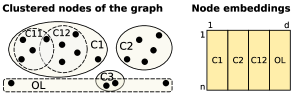
Figure 1: Transformation of the hierarchy of overlapping clusters consisting of $n$ nodes and $k=5+2$ clusters (2 nodes-outliers, which are grouped as OL together with the outlier cluster C3) into $d=4$ dimensional node embeddings.

IV-A Feature Extraction from Clusters

Intuitively, a straightforward approach for feature extraction from clusters is to consider each cluster as a dedicated feature representing one embedding dimension [24]. This approach can be used to discriminate between the nodes (given a fine-grained structure of clusters), but on the other hand, may not correlate with the graph embedding objective of providing a low-dimensional representation of the nodes. Fixing the number of clusters to the required number of dimensions $d$ is possible when considering flat clustering [24] but not for hierarchical cases. For hierarchical clustering, producing $d$ dimensions can be expressed with an inequality in the general case, i.e. producing at most $d$ clusters at the top level. Therefore, some technique to identify a small number $s\geq d$ of salient clusters, which are then regarded as features, is required. This number $s$ can either be parameterized or, ideally, inferred as the optimal tradeoff between the number of clusters and their quality. In addition, there exists a fundamental constraint on the structure of the clusters used to create the embedding space. Namely, each graph node should be connected to at least one feature to be present in the embeddings.

The exact way salient clusters (features) are identified depends on the structure of the clusters (e.g., hierarchical, multi-resolution, overlapping, non-overlapping) and on the ability to control the number of formed clusters $k\geq s$ by the community detection algorithm. In the following, we discuss salient clusters identification for the most general case, i.e., for clustering techniques that are multi-resolution, hierarchical and overlapping.

Algorithm 1 Features extraction

1:function features($hier$)

2:    $scls\leftarrow[]$ $\triangleright$ Salient clusters (features), dynamic array

3:    $clsts\leftarrow\{\}$ $\triangleright$ Ancestor cluster statistics, hash map

4:    for all $lev\in hier$ do

5:         for all $cl\in lev$ do

6:             $res\leftarrow\texttt{count}(cl.ances)=0$ $\triangleright$ Salient flag

7:             $dens\leftarrow cl.weight/\texttt{count}(cl.nodes)$ $\triangleright$ Density

8:             $savdens\leftarrow 0;savwgh\leftarrow 0$ $\triangleright$ Statistics to be stored

9:             if not $res$ then

10:                 $hits\leftarrow 0$ $\triangleright$ Saliency hits

11:                 for all $ac\in cl.ances$ do $\triangleright$ Traverse ancestors

12:                     $ast\leftarrow clsts[ac]$ $\triangleright$ Ancestor statistics

13:                     if $savdens<ast.dens$ and (not $savwgh$ or $savwgh>ast.wgh$) then

14:                         $savdens\leftarrow ast.dens$

15:                         $savwgh\leftarrow ast.wgh$

16:                     end if

17:                     if not $res$ and $dens\geq ast.dens$ and $cl.weight\leq ast.wgh$ then

18:                         $hits\leftarrow hits+1$

19:                     end if

20:                     $ast.reqs\leftarrow ast.reqs+1$

21:                     if $ast.reqs=\texttt{count}(ac.des)$ then

22:                         $clsts.erase(cl)$ $\triangleright$ Remove outdated

23:                     end if

24:                 end for

25:             end if

26:             if not $res$ and $hits=\textbf{count}(cl.ances)$ then

27:                 $res\leftarrow$ true

28:             end if

29:             $savwgh\leftarrow cl.weight*wrstep$

30:             $clsts[cl]\leftarrow(savdens,savwgh)$ $\triangleright$ dens,wgh,reqs=0

31:             if $res$ then

32:                 $scls.add(cl)$

33:             end if

34:         end for

35:    end for

36:    return $scls$ $\triangleright$ The resulting salient clusters

37:end function

Features extraction is presented in Algorithm 1. We traverse all clusters on each level of the formed hierarchy of clusters starting from the top level, and fetch as salient clusters: a) the top-level clusters of the hierarchy (line 6) (to cover all nodes) and b) all the nested clusters satisfying the following requirements (line 17):
- having a higher weight density than each of their direct super-clusters (ancestors), since the nested salient clusters are expected to represent the mutual core structure [44] of their ancestors, and
- weighting less than the most lightweight ancestor (discounted by a factor).
The weight discounting factor $r_{w}$ (line 29) is required to prevent fetching too many similar clusters that are nested into each other. The factor $r_{w}\in[0.5,1)$ retains an approximation of the nested cluster to its ancestor, while $r_{w}\rightarrow r_{w_{min}}=0.5$ reduces the number of salient clusters. However, considering the availability of overlapping clusters and known weight of the overlap $w_{C_{ovp}}<w_{C}$ for the cluster $C$, we refine $r_{w}$ as $r_{w}=0.5+\frac{(b-1)\times w_{c_{ovp}}}{2\,b\times w_{c}}$, where $b\geq 2$ is the overlap factor equal to the number of clusters sharing the overlapping nodes in $C$. Also, the number of overlapping clusters can be estimated according to the Pareto principle [45, 46], which makes reasonable to take $r_{w}=0.5\times 1.2=0.6$ when the exact value cannot be evaluated.

IV-B Dimension Formation from Features

Embedding dimensions are formed from the salient clusters extracted above, which implicitly yields the recommended number of dimensions for the input graph based on its statistical properties. The embedding vector $v_{i}\in V$ of size $d=|D|$ for each graph node #i is then produced by quantifying the degree of belonging of the node to each dimension $D_{j}$ as the node weight $w_{i,D_{j}}$ belonging to this dimension. This weight corresponds to the aggregated weight of the node links to other nodes being members of all salient clusters composing the dimension:

$$\begin{split}V=\{\frac{w_{i,D_{j}}}{w_{i}}\;|\;i=1..n,j=1..d\},\\ w_{i,D_{j}}=\sum_{k\in nodes(D_{j})}w_{i,k}\,.\end{split}$$ (5)

We perform this embedding vectors generation efficiently by resorting to a single scan over the members of each salient cluster. The node weights are then aggregated to form the dimension values. The embedding vectors are obtained by transposing the resulting matrix: $V=D^{T}$.

Constraining the Number of Dimensions

In the case of a connected graph without clusters-outliers, the most salient clusters $d$ are fetched from the $t\leq d\leq s$ top level clusters of the hierarchy and from the $d-t$ densest of the remaining $s-t$ salient clusters. When the clustering algorithm does not allow to control the number of top level clusters or when the graph is disconnected and the number of components is larger than $d$ resulting in $t>d$, then the dimensions are formed as follows. According to the so-called “Rag Bag” formal constraint of clustering quality [47, 48], the $t-(d-1)$ most lightweight clusters should be grouped together to the last dimension and the $d-1$ heaviest clusters fill the remaining dimensions. However, the presence of outliers on the top levels prevents to effectively generate dimensions from the salient clusters. To solve this issue, the outliers can be separated from the valid clusters based on their weights, which are either evaluated from the statistical distributions or approximately estimated as follows. In case there is no prior information about the data, a rule of thumb is to take the estimated minimal size of clusters as the square root of the number of nodes [49]. Generalizing the rule of thumb to the weighted graphs, the number of $z<t$ root clusters, each having a weight less that the square root of the graph weight $w$ can be moved to the “outliers” dimension. The resulting dimensions are composed of the $t-z$ top level clusters of the hierarchy, the $d-1-(t-z)$ densest remaining salient clusters, each having a weight $w_{i}\geq\sqrt{w}$, and a single dimension of outliers to cover all remaining graph nodes (see Fig. 1 for an illustration).

Dimension Interpretability

The resulting embedding space is inherently easier to interpret than spaces derived from other techniques, as its dimensions are taken from (salient) clusters representing ground-truth semantic categories, with accuracy being evaluated using extrinsic quality metrics [47]. This opens the door to new features and applications in the fields of granular and privacy-preserving computations. For example, only a subset of the dimensions having some required semantics can be fetched for evaluation, which has the advantage of reducing the amount of processing data while avoiding to leak or share information beyond the required features.

V Community Detection

In this section, we first discuss the properties of a community detection algorithm that are required to perform an effective and efficient graph embedding. Then, we select one of the most suitable state-of-the-art community detection algorithms for our task and propose its extension to satisfy the required properties.

As an effective graph embedding technique should preserve both low- and high-order node proximities, the community detection algorithm used for the graph embedding should be able to produce clusters with various resolutions (i.e., at different granularities). Moreover, the more resolutions are covered, the wider the range of node proximity orders that can be captured, since each embedding dimension consists of at least one cluster as described in Section IV-B. A low-dimensional representation of graph nodes implies a small number $t$ of coarse-grained (macro-scale) clusters, since the number of generated dimensions $d\geq t$ (see Section IV). This number $t$ should be a parameter of the technique when a specific number $d$ of embedding dimensions is required, with a default value defined according to the statistical properties of the input graph.

In addition, the following properties of community detection algorithms are also required to generate high-quality embeddings, to simplify and speedup the generation process:

• Each graph node should potentially belong to multiple features (i.e., should be represented in multiple dimensions), which requires the clustering to be soft (i.e., fuzzy or overlapping).

• It is desirable to have graph embedding techniques applicable to any input graph without any manual tuning; hence, the clustering should be parameter-free and efficient (to be applicable to large graphs).
  - An unsupervised parameter-free processing is sensitive to the quality of the input data, so a robust clustering algorithm is required. Robustness is typically reached by applying a consensus (also called ensemble) clustering method [50, 51, 52].
  - From a practical perspective, it is desirable to have consistent embeddings for the same input graph irrespective of the order in which the nodes are processed or whether their IDs are modified. The clustering algorithm should hence be deterministic and input-order invariant.
  - Considering the hierarchical nature of complex networks modeling real-world systems [37, 53], the effective clustering algorithm should be hierarchical. In particular, an agglomerative hierarchical clustering addresses also the efficiency criterion by reducing the number of processed items at each iteration, since each hierarchy level is built using clusters from the previous level directly.

Following the above requirements, DAOCftn:daoc [13] is, to the best of our knowledge, the only parameter-free clustering algorithm that is simultaneously deterministic, input order invariant, robust (as it uses a consensus approach) and applicable to large weighted networks yielding a fine-grained hierarchy of overlapping clusters [54]. Moreover, it is based on a MMG meta-optimization function, where generalized modularity gain can be used as the target optimization function to perform clustering at the required resolution. However, DAOC a) yields a hierarchy of clusters only for a single value of the resolution parameter ($\gamma=1$ operating with the non-generalized modularity), treating the hierarchy levels as scales (i.e., resolutions in terms of nested clusters rather than distinct values of $\gamma$) similar to [55, 12], and b) does not bound the size of the top (root) level of the forming hierarchy to produce the required number $t\leq d$ of clusters as described in Section IV-A. Therefore, we propose two extensions addressing these issues in the following.

V-A Hierarchical multi-resolution clustering

Even though a multi-resolution structure of non-overlapping clusters is not necessary hierarchical [56, 57] (i.e., a node might be a member of several clusters that are not nested into each other), it can be represented as a hierarchy of overlapping clusters [58] (where the overlap addresses the case of a node shared by non-nested clusters). However, a hierarchical overlapping structure created with a single resolution may substantially differ from the respective multi-resolution structure (i.e., the produced clusters may differ vastly) as illustrated in Fig. 2, where the strength on nodes interaction is represented with the width of the links and the number of interactions with the size of the nodes (i.e., their weight). A large value of the resolution parameter can penalize heavily-weighted nodes according to Eq. (3), resulting in grouping together linked lightweight nodes. Such a behavior makes sense in many real-world cases, for example when employees working on the same project interact more frequently with their supervisor than between each other but the supervisor may not be a core of the group, participating also in other projects. Therefore, it is essential to incorporate the resolution parameter when generating the hierarchy levels, similar to [56, 59, 60].

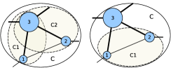
Figure 2: A possible overlapping hierarchical clustering with the fixed resolution parameter of the weighed subgraph consisting of three nodes is shown on the left-hand side of the figure. A possible multi-resolution clustering for the same subgraph is shown on the right-hand side. The size of the nodes and the width of the links correspond to their weights.

In [56, 60], the authors operate with the analog of the resolution parameter called resistance parameter, which can not be transformed to the resolution parameter $\gamma$ according to [42] and, hence, cannot be used with the generalized modularity defined in Eq. (3). In [59], the scale factor $\alpha$ is proposed, which can be directly transformed to the resolution parameter: $\gamma=(1-\alpha)/\alpha$. However, the computational complexity of the proposed method is $O(n\sqrt{n})\times O_{0}$ in average and $O(n^{2})\times O_{0}$ in the worst case, where $n$ is the number of nodes in the graph and $O_{0}$ is the complexity of the original clustering algorithm without the multi-scaling technique. This boosting of the computational complexity makes this technique inappropriate for large graphs. Hence, we propose our own approach to produce a hierarchy of multi-resolution clusters for large graphs based on DAOC.

The main idea behind our efficient multi-resolution hierarchical clustering is the dynamic variation of the resolution parameter $\gamma$ during the hierarchy construction process. More precisely, DAOC is an agglomerative clustering algorithm, which builds the hierarchy bottom-up with micro-scale clusters on the bottom levels. These clusters should be constructed on a high value of the resolution parameter ($\gamma\gg 1$) according to Eq. (3). The resolution should then gradually decrease to the lowest value $\gamma>0$ yielding macro-scale clusters located on the top (root) level of the hierarchy. The bounds for $\gamma$ can be estimated based on the resolution limit analysis conducted in [40], where the equation is defined for the marginal case when all clusters have a perfect balance between the internal and external degrees being on the limit of detectability. That equation takes the following shape when adapted to the generalized modularity:

$$\check{\dot{m}}<\check{\dot{m}}_{max}=\frac{m}{4\gamma},$$ (6)

where $\check{\dot{m}}$ is the number of internal links in a cluster and $m$ is the total number of links in the graph. To estimate the upper bound of $\gamma$, we need to bind $\check{\dot{m}}$ and $m$, which could be done relying on the two following heuristics. First, in case there is no prior information about the data, a rule of thumb is to take the estimated maximal number of clusters as the square root of the number of nodes [49]: $\tilde{k}_{max}=\sqrt{n}$. Then, considering that the number of internal links constitutes half of all the links of a cluster in the marginal case described by Eq. (6):

$$2\,m=2\,\check{\dot{m}}\times k,\;k\lesssim\tilde{k}_{max}\implies m\lesssim\check{\dot{m}}\sqrt{n}.$$ (7)

Second, most real-world systems are modeled by sparse graphs [53]. The number of links in a sparse graph does not exceed $n^{3/2}$. Thereby, Eq. (6) extended with Eq. (7) takes the following shape:

$$\check{\dot{m}}<\frac{\check{\dot{m}}\sqrt{n}}{4\gamma}\implies\gamma<\frac{\sqrt{n}}{4}\lesssim\frac{\sqrt[3]{m}}{4}\leq\frac{\sqrt[3]{w/\breve{w}_{min}}}{4}=\gamma_{max}.$$ (8)

where $\breve{w}_{min}$ is the minimal weight of a link. Eq. (8) provides a definition for the upper bound of $\gamma$ in a weighted graph. The lower bound of gamma is evaluated dynamically based on the optimal value of the resolution parameter given in Eq. (4) for each level of the hierarchy: $\gamma_{min}=\acute{\gamma}$. Typically, $\acute{\gamma}\geq 1$ for large real-world networks [34], so $\gamma_{min}=0.5\,..\,1$ is taken for the first iteration before $\acute{\gamma}$ is evaluated.

In summary, $\gamma$ is decreased from $\gamma_{max}$ to $\gamma_{min}$ with a fixed ratio $r_{\gamma}$ and represents a trade-off between the number of captured resolutions when $r_{\gamma}\rightarrow 1$ versus a lower number of iterations (i.e., higher efficiency) and higher quality on coarse resolutions when $r_{\gamma}\rightarrow 0$. The quality of the forming macro-clusters is affected by the amount and size of the fine-grained clusters since the former are constructed iteratively from the latter, and the actual multi-resolution structure is not necessary hierarchical [56, 57]. In theory, $r_{\gamma}$ should allow the growth of the cluster weight by a factor less than two to still retain the cluster semantics (super/sub-cluster ordering). Otherwise, the super/sub-cluster association is transformed into an overlapping clusters relation, losing the hierarchical structure. The limitation of the cluster weight growth to a factor 2 corresponds to $r_{\gamma}>2^{-2}=0.25$ according to Eq. (3), which is a hard theoretical bound. In practice, a larger value of $r_{\gamma}$ is required considering the possibility of multiple mutually overlapping clusters as discussed in Section IV-A: $r_{\gamma}\gtrsim r_{w_{min}}^{2}=0.36$. The upper bound of $r_{\gamma}$ corresponds to the lower bound of the cluster weight growth factor, which can be taken as $10-20\%$ according to the Pareto principle [45, 46] or 10/90 gap [61]: $r_{\gamma}\leq 1.1^{-2}=0.826$. Thus, the operational range of the gamma ratio is as follows: $r_{\gamma}\in[0.36,0.826]$, and we pick $r_{\gamma}=0.6$. This selected value is not supposed to be tuned by the users. Higher values of $r_{\gamma}$ yield a larger number of salient clusters, which is not desirable, and lower values may cause the loss of some important salient clusters. The exact theoretical $r_{\gamma}$ depends on the number of overlapping clusters on the next iteration, which is generally speaking unknown.

V-B Bounding the number of clusters

DAOC generates a hierarchy of clusters as long as the value of the optimization function is improving (i.e., $\Delta Q\geq 0$), which might result in any number of clusters at the top level of the hierarchy. If a specific number of clusters is required (e.g., for a fair comparison of various graph embedding techniques on the same number of dimensions), we propose the following extensions of the hierarchy generation process:

• The hierarchy generation is interrupted early if the number of clusters at level $i$, $|h_{i}|$ reaches the required number $d$.

• The hierarchy generation is forced to continue until the number of clusters reaches the required number $d$ even if the value of the optimization function $\Delta Q$ becomes negative. In that case, the clustering objective becomes the minimal loss of the optimization function value: $\max\Delta Q<0$.

The proposed extensions of the clustering algorithm are summarized in Algorithm 2. The early termination of the hierarchy construction process happens on lines 11, 19. The forced continuation of the hierarchy construction corresponds to a boolean parameter $d\neq 0$ for the original DAOC clustering on line 7. This parameter prevents the completion of the clustering process when the optimization function $\Delta Q$ cannot be further improved.

Algorithm 2 Hierarchical multi-resolution clustering with optionally bounded number of clusters.

1:function cluster($nodes,d$)

2:    $rg\leftarrow 0.6$ $\triangleright$ Gamma ratio

3:    $gamma\leftarrow\sqrt[3]{\texttt{weight}(nodes)/\texttt{min\_weightln}(nodes)}/4$

4:    $gmin\leftarrow 0.5$ $\triangleright$ Min gamma

5:    $hier\leftarrow[]$ $\triangleright$ List of the hierarchy levels

6:    while $nodes$ do $\triangleright$ Stop if the nodes list is empty

7:         $cls\leftarrow\texttt{daocHierLev}(nodes,gamma,d)$

8:         if $gamma*(rg+1)/2\geq gmin$ and (not $cls$ or $\texttt{count}(cls)\leq\sqrt{\texttt{count}(nodes)}$) then $\triangleright$ Decrease gamma

9:             $gamma\leftarrow gamma*rg$

10:         else

11:             $nodes\leftarrow cls$ $\triangleright$ Consider early termination

12:         end if

13:         if $cls$ then $\triangleright$ Initialize the next-level nodes

14:             $hier.append(cls)$ $\triangleright$ Extend the hierarchy

15:             $gmin\leftarrow\texttt{gammaOptim}(cls)$ $\triangleright$ Update min gamma

16:             if not $d$ or $\texttt{count}(cls)>d$ then

17:                 $nodes\leftarrow cls$ $\triangleright$ Update the processing nodes

18:             else

19:                 $nodes\leftarrow[]$ $\triangleright$ Early termination

20:             end if

21:         end if

22:    end while

23:    return $hier$ $\triangleright$ The resulting hierarchy of clusters

24:end function

VI Experimental Evaluation

In this section, we conduct an extensive set of experiments to evaluate our proposed method on two typical graph analysis tasks, i.e., node classification and link prediction. We start by introducing our experimental setup including the datasets and baselines we use before presenting our experimental results.

VI-A Experimental Setup

VI-A1 Datasets

We conduct experiments on the following five graphs, which are widely used in the current literature for evaluating graph embedding techniques. Table II summarizes the key characteristics of the graphs.
$\bullet$ BlogCatalog (Blog) [24] is a social network of bloggers. Each node represents a user, while the labels of a node represent the topics the corresponding user is interested in.
$\bullet$ Protein-Protein Interactions (PPI) [3] is a graph of the PPI network for Homo Sapiens. The labels of a node refer to its gene sets and represent the corresponding biological states.
$\bullet$ Wikipedia (Wiki) [3] is a co-occurrence network of words appearing in a sampled set of the Wikipedia dump. The labels represent part-of-speech tags.
$\bullet$ DBLP [62] is a collaboration network capturing the co-authorship of writers. Each node represents an author, and the labels of a node refer to the publication venues of the corresponding author.
$\bullet$ YouTube [63] is a social network of users on YouTube. Each node represents a user, and the labels of a node refer to the groups (e.g., “anime”) that the corresponding user is interested in. This graph is used only to evaluate the efficiency of the embedding techniques, since the ground-truth categories include only 3% of the graph (as opposed to a 100% coverage for the other graphs).

TABLE II: Characteristics of the experimental graphs

Dataset	Blog	PPI	Wiki	DBLP	YouTube
Nodes	10,312	3,890	4,777	13,326	1,138,499
Links	333,983	76,584	184,812	34,281	2,990,443
Labels	39	50	40	2	47

VI-A2 Baselines

We compare our proposed technique against ten state-of-the-art graph embedding techniques from three categories.

Graph-sampling based techniques

DeepWalk [2], Node2Vec [3], LINE [16] and VERSE [64]. For DeepWalk and Node2Vec, we set the walk length to 40, the number of walks per node to 80, and the context window size to 10. For Node2Vec, we also tune the return parameter $p$ and the in-out parameter $q$ with a grid search over $p,q\in\{0.25,0.05,1,2,4\}$. For LINE, we set the total number of samples to 1 billion for Blog, PPI, Wiki and DBLP and to 10 billions for YouTube. For VERSE, we tune the damping factor $\alpha$ of personalized PageRank using the method suggested by the authors.

Factorization-based techniques

GraRep [17], HOPE [4] and NetMF [5]. For GraRep, we search the optimal $k$ over $\{1,2,3,4,5,6\}$. When $d/k$ is not an integer, we learn the first $k-1$ sets of $\lceil d/k\rceil$-dimension embeddings, and the last set of embeddings of dimension $d-(k-1)\lceil d/k\rceil$. For HOPE, we search the optimal decay parameter $\beta$ from $0.1$ to $0.9$ with a step of $0.2$. For NetMF, we tune the implicit window size $T$ within $\{1,10\}$.

Similarity-preserving hashing based techniques

INH-MF [65], NetHash [18] and NodeSketch [19]. For INH-MF, we set the ratio for subspace learning to 100%, to let it achieve optimal performance w.r.t. the quality of the learnt node embeddings. For NetHash, as suggested by the authors, we search the optimal tree depth in $\{1,2,3\}$. For NodeSketch, we search the optimal order of proximity $k$ up to $6$ and the optimal decay parameter $\alpha$ from $0.0001$ to $1$ on a log scale.

Meta techniques

HARP [20]. We configure HARP to learn from the embeddings of DeepWalk (HARP-DWalk) and LINE (HARP-LINE) using the following parameter settings. For HARP-DWalk, we set the walk length to 10, the number of walks per node to 40, the context window size to 10 and the sampling ratio to 0.1. For HARP-LINE, we set the context window size to 1, the number of iterations to 50 and the sampling ratio to 0.001.

VI-B Node Classification Task

Node classification tries to predict the most probable label(s) for some nodes based on other labeled nodes. In this experiment, we consider a multi-label setting, where a node is assigned one or multiple labels. Our evaluation was performed using an open-source graph embeddings evaluation framework, GraphEmbEval, which uses the same evaluation scheme as in [2, 3, 17]. More precisely, we randomly pick a set of nodes as labeled nodes for training, and use the rest for testing. To fairly compare node embeddings with different similarity measures, we train a one-vs-rest kernel SVM classifier with a pre-computed kernel (cosine, Jaccard or Hamming kernel according to the embedding techniques) to return the most probable labels for each node. We report the average Macro-F1 and Micro-F1 scores from 5 repeated trials. A higher value of these metrics implies better performance.

TABLE III: Node classification performance using kernel SVM, where the top-3 results for each dataset are highlighted with bold numbers

Method	Micro-F1 (%)				Macro-F1 (%)
	Blog	PPI	Wiki	DBLP	Blog	PPI	Wiki	DBLP
$\cdot$DeepWalk	39.60	17.24	46.05	83.46	21.93	10.28	6.62	83.16
:Node2Vec	37.95	16.04	50.32	93.25	20.22	9.57	9.86	93.12
$\cdot$LINE	35.49	15.01	48.22	86.83	16.60	8.70	8.47	86.54
$\cdot$VERSE	39.61	15.90	41.39	92.79	22.85	9.76	4.14	92.66
:GraRep	36.21	5.83	56.22	91.41	16.91	1.52	12.14	91.25
:HOPE	31.37	14.69	56.68	91.47	11.74	8.13	13.30	91.30
:NetMF	40.04	15.03	57.62	93.59	23.43	8.74	14.35	93.46
$\cdot$INH-MF	36.13	15.50	45.03	93.27	18.88	9.55	6.90	93.16
:NetHash	35.80	18.85	47.57	97.61	18.72	12.91	8.05	97.57
:NodeSketch	38.16	21.04	59.07	98.83	21.84	15.55	16.31	98.81
$\cdot$HARP-DWalk	36.52	15.46	43.06	92.66	19.56	9.04	5.59	92.53
$\cdot$HARP-LINE	30.27	12.67	42.79	88.07	13.06	6.25	5.38	87.84
DAOC	21.3	12.56	42.43	89.24	6.47	7.25	5.66	89.03
DAOR	33.05	19.07	53.24	87.86	17.25	13.94	15.97	87.64

$\cdot$ the algorithm meta parameters are tuned once for all datasets to maximize accuracy
: the algorithm parameters are tuned for each dataset to maximize accuracy

Our method, DAOR, shows competitive results without requiring any tuning (unlike conventional embedding techniques, which require extensive tuning, as described above). We also evaluated embeddings generated using DAOC without our proposed extension for multi-resolution clustering. The improvement of DAOR over DAOC verifies the effectiveness of our proposed extensions for graph embedding.

VI-C Link Prediction Task

Link prediction is a typical graph analysis task that predicts potential (or missing) links between nodes in a graph. For this task, we use the same setting as in [4]. Specifically, we randomly sample 20% of the links out of the graph as test data, and use the rest of the graph for training. After learning the node embeddings based on the training graph, we predict the missing links by generating a ranked list of potential links. For each pair of nodes, we use the cosine, Jaccard or Hamming similarity (according to the embedding techniques) between their embedding vectors to generate the ranked list. As the number of possible pairs of nodes is too large, we randomly sample 0.1% pairs of nodes for evaluation. We report the average precision@N and recall@N from 10 repeated trials.

TABLE IV: Link prediction performance, where the top-3 results for each dataset are highlighted with bold numbers

Method	Precision@100				Recall@100
	Blog	PPI	Wiki	DBLP	Blog	PPI	Wiki	DBLP
$\cdot$DeepWalk	0.0200	0.0159	0.0090	0.0423	0.0301	0.2227	0.0493	0.6749
:Node2Vec	0.0927	0.0137	0.0267	0.0321	0.1378	0.1958	0.1514	0.5174
$\cdot$LINE	0.0070	0.0073	0.0031	0.0392	0.0103	0.0923	0.0167	0.6186
$\cdot$VERSE	0.0404	0.0206	0.0212	0.0436	0.0602	0.2723	0.1118	0.6906
:GraRep	0.0014	0.0011	0.0054	0.0001	0.0020	0.0118	0.0286	0.0011
:HOPE	0.0023	0.0073	0.0027	0.0248	0.0035	0.0960	0.0149	0.4034
:NetMF	0.0175	0.0174	0.0084	0.0218	0.0266	0.2287	0.0474	0.3126
$\cdot$INH-MF	0.0158	0.0158	0.0084	0.0252	0.0227	0.2209	0.0454	0.4052
:NetHash	0.0015	0.0134	0.0020	0.0387	0.0022	0.1899	0.0101	0.5958
:NodeSketch	0.0729	0.0250	0.0176	0.0462	0.1080	0.3331	0.0942	0.7595
$\cdot$HARP-DWalk	x	0.0142	0.0101	0.0407	x	0.1978	0.0536	0.6459
$\cdot$HARP-LINE	x	0.0026	0.0021	0.0309	x	0.0331	0.0117	0.5029
DAOC	0.0001	0.0099	0.0059	0.0027	0.0001	0.1301	0.0314	0.0444
DAOR	0.0958	0.0175	0.0164	0.0032	0.1438	0.2345	0.0892	0.0548

$\cdot$ the algorithm meta parameters are tuned once for all datasets to maximize accuracy
: the algorithm parameters are tuned for each dataset to maximize accuracy
x the algorithm is crashed on coarsening small disconnected components

Table IV shows the results of the link prediction task. Our proposed method, DAOR, is among the top-3 best-performing techniques being unsupervised and parameter-free. The impact of our proposed multi-resolution clustering is especially visible on this task, were DAOR significantly outperforms DAOC.

VI-D Robustness to the Metric Space

Node embedding robustness to different metric spaces is shown in Table V on the node classification task for our method DAOR versus the two other best-performing methods from Table III that technically can be evaluated with another metric space (NodeSketch is omitted because it uses a non-linear Hamming metric space, where cosine distance cannot be formally evaluated). For all input graphs, DAOR shows the best worst-case performance, i.e., DAOR yields much more accurate results in its least accurate non-primary metric space than the other methods do. Moreover, Hamming distance is directly applicable to DAOR without any preliminary binarization, unlike the algorithms operating in the cosine metric space.

TABLE V: Node embedding robustness to the metric space, where the native metric space for each algorithm is highlighted in bold

Method	Metric	Micro-F1 (%)
		Blog	PPI	Wiki	DBLP
DAOR	jaccard	33.05	19.07	53.24	87.86
	cosine	30.41	13.62	47.20	87.42
	hamming	23.87	14.13	45.52	86.98
	binham	23.89	10.25	41.36	87.17
NetMF	cosine	40.04	15.03	57.62	93.59
	hamming	17.54	6.55	40.93	70.32
	binham	19.82	7.05	42.85	74.91
HOPE	cosine	31.37	14.69	56.68	91.47
	hamming	17.02	5.95	40.89	59.94
	binham	18.23	6.21	40.89	74.36

binham - Hamming metric applied after a binarization of each dimension using its median value

VI-E Runtime Performance

In this experiment, we investigate the efficiency of the graph embedding learning process. Our evaluation was performed using an open-source graph embeddings evaluation framework, GraphEmbEvalftn:gembev. on a Linux Ubuntu 16.04.3 LTS server with an Intel Xeon CPU E5-2620 v4 @ 2.10GHz CPU (16 physical cores) and 132 GB RAM. The training and execution termination constraints for each algorithm were set to 64 GB of RAM and 240 hours CPU time (we terminate the process when either of those thresholds are met).

TABLE VI: Node embedding learning time (in seconds), where the top 3 results for each dataset are highlighted in bold

Method	Blog	PPI	Wiki	DBLP	YouTube
DeepWalk	3375	1273	1369	4665	747060
Node2Vec	1073	383	1265	504	-
LINE	2233	2153	1879	2508	29403
VERSE	1095	203	276	1096	245334
GraRep	3364	323	422	10582	-
HOPE	239	100	78	283	15517
NetMF	487	124	708	213	-
INH-MF	509	39	98	378	-
NetHash	721	201	134	35	12708
NodeSketch	70	8	17	8	2439
HARP-DWalk	1436	299	483	958	336200
HARP-LINE	1274	106	189	90	13951
DAOC	7.9	0.3	1.8	0.2	4893
DAOR	1.6	0.2	0.4	0.2	57.1

- the algorithm was terminated by timeout

Table VI shows the end-to-end embedding learning time. To discount the impact of the multi-threaded implementation of some of the methods, we dedicate a single logical CPU per each method implementation and report the total CPU time. Our method, DAOR, is faster than existing state-of-the-art techniques by several orders of magnitude; it exhibits near-linear scaling when increasing the number of links in the graph. DAOR is also much more scalable than DAOC (on which DAOR is built) due to its specific multi-scaling approach that boosts the number of nodes reaching consensus of the optimization function early on lower levels of the hierarchy. Moreover, unlike other graph embedding techniques, DAOR execution time decreases when increasing the number of embedding dimensions, which is due to the early termination of the clustering as described in Section V-B.

VII Conclusions

In this paper, we presented a novel highly efficient and parameter-free graph embedding technique, DAOR ftn:sys, which produces metric-robust and interpretable embeddings without requiring any manual tuning. Compared to a dozen state-of-the-art graph embedding algorithms, DAOR yields competitive results on diverse graph analysis tasks (node classification and link prediction), while being several orders of magnitude more efficient.

In future work, we plan to recommend the minimal, maximal and optimal number of embedding dimensions, and conduct a comprehensive study on their quality and interpretability. Also, we plan to integrate further state-of-the-art community detection algorithms in addition to DAOC.

References

- [1] H. Cai, V. W. Zheng, and K. Chang, “A comprehensive survey of graph embedding: problems, techniques and applications,” TKDE, 2018.
- [2] B. Perozzi, R. Al-Rfou, and S. Skiena, “Deepwalk: Online learning of social representations,” in KDD’14. ACM, 2014, pp. 701–710.
- [3] A. Grover and J. Leskovec, “node2vec: Scalable feature learning for networks,” in KDD’16. ACM, 2016, pp. 855–864.
- [4] M. Ou, P. Cui, J. Pei, Z. Zhang, and W. Zhu, “Asymmetric transitivity preserving graph embedding,” in KDD’16. ACM, 2016, pp. 1105–1114.
- [5] J. Qiu, Y. Dong, H. Ma, J. Li, K. Wang, and J. Tang, “Network embedding as matrix factorization: Unifying deepwalk, line, pte, and node2vec,” in WSDM’18. ACM, 2018, pp. 459–467.
- [6] L. Katz, “A new status index derived from sociometric analysis,” Psychometrika, vol. 18, no. 1, pp. 39–43, 1953.
- [7] Y. Y. Yao, “Granular computing: basic issues and possible solutions,” in 5th Joint Conference on Information Sciences, 2000, pp. 186–189.
- [8] M. E. J. Newman, “The structure and function of complex networks,” SIAM Rev., vol. 45, no. 2, 2003.
- [9] S. Cavallari, V. W. Zheng, H. Cai, K. C.-C. Chang, and E. Cambria, “Learning community embedding with community detection and node embedding on graphs,” in CIKM. ACM, 2017, pp. 377–386.
- [10] X. Wang, P. Cui, J. Wang, J. Pei, W. Zhu, and S. Yang, “Community preserving network embedding,” in AAAI, 2017.
- [11] D. Yang, B. Li, L. Rettig, and P. Cudré-Mauroux, “Histosketch: Fast similarity-preserving sketching of streaming histograms with concept drift,” in ICDM’17. IEEE, 2017, pp. 545–554.
- [12] V. D. Blondel, J.-L. Guillaume, R. Lambiotte, and E. Lefebvre, “Fast unfolding of communities in large networks,” J Stat Mech., no. 10, 2008.
- [13] A. Lutov, M. Khayati, and P. Cudré-Mauroux, “Daoc: Stable clustering of large networks,” in IEEE BigData, 2019.
- [14] D. Yang, B. Qu, J. Yang, and P. Cudre-Mauroux, “Revisiting user mobility and social relationships in lbsns: a hypergraph embedding approach,” in WWW. ACM, 2019, pp. 2147–2157.
- [15] R. Hussein, D. Yang, and P. Cudré-Mauroux, “Are meta-paths necessary?: Revisiting heterogeneous graph embeddings,” in CIKM, 2018, pp. 437–446.
- [16] J. Tang, M. Qu, M. Wang, M. Zhang, J. Yan, and Q. Mei, “Line: Large-scale information network embedding,” in WWW, 2015, pp. 1067–1077.
- [17] S. Cao, W. Lu, and Q. Xu, “Grarep: Learning graph representations with global structural information,” in CIKM’15. ACM, 2015, pp. 891–900.
- [18] W. Wu, B. Li, L. Chen, and C. Zhang, “Efficient attributed network embedding via recursive randomized hashing.” in IJCAI, 2018.
- [19] D. Yang, P. Rosso, B. Li, and P. Cudre-Mauroux, “Nodesketch: Highly-efficient graph embeddings via recursive sketching.” in KDD, 2019.
- [20] H. Chen, B. Perozzi, Y. Hu, and S. Skiena, “Harp: Hierarchical representation learning for networks,” in AAAI, 2018.
- [21] L. Tang and H. Liu, “Leveraging social media networks for classification,” Data Min. Knowl. Discov., vol. 23, pp. 447–478, Nov. 2011.
- [22] M. Fiedler, “Algebraic connectivity of graphs,” Czechoslovak Mathematical Journal, vol. 23, no. 2, pp. 298–305, 1973.
- [23] A. Pothen, H. Simon, and K. Liou, “Partitioning sparse matrices with eigenvectors of graphs,” SIMAX, vol. 11, no. 3, pp. 430–452, 1990.
- [24] L. Tang and H. Liu, “Relational learning via latent social dimensions,” in ACM SIGKDD. ACM, 2009, pp. 817–826.
- [25] M. E. J. Newman, “Finding community structure in networks using the eigenvectors of matrices,” Phys. Rev. E, vol. 74, p. 036104, Sep 2006.
- [26] C. Ding, X. He, and H. D. Simon, “On the equivalence of nonnegative matrix factorization and spectral clustering,” in SDM, 2005, pp. 606–610.
- [27] J. Yang and J. Leskovec, “Overlapping community detection at scale: A nonnegative matrix factorization approach,” ser. WSDM, 2013.
- [28] H. Zhang, C. L. Giles, H. C. Foley, and J. Yen, “Probabilistic community discovery using hierarchical latent gaussian mixture model,” ser. AAAI, vol. 1, 2007, pp. 663–668.
- [29] D. Wang, P. Cui, and W. Zhu, “Structural deep network embedding,” ser. ACM SIGKDD, 2016, pp. 1225–1234.
- [30] M. E. J. Newman, “Fast algorithm for detecting community structure in networks,” Phys. Rev. E, vol. 69, p. 066133, Jun 2004.
- [31] T. A. Snijders and K. Nowicki, “Estimation and prediction for stochastic blockmodels for graphs with latent block structure,” Journal of Classification, vol. 14, no. 1, pp. 75–100, Jan 1997.
- [32] L. Yu and C. Ding, “Network community discovery: Solving modularity clustering via normalized cut,” ser. MLG ’10. ACM, pp. 34–36.
- [33] M. E. J. Newman, “Spectral methods for network community detection and graph partitioning,” Phys. Rev. E, vol. 88, no. 4, p. 042822, 2013.
- [34] Newman, M. E. J., “Equivalence between modularity optimization and maximum likelihood methods for community detection,” Phys. Rev. E, vol. 94, p. 052315, 2016.
- [35] B. Karrer and M. E. J. Newman, “Stochastic blockmodels and community structure in networks,” Phys. Rev. E, vol. 83, Jan 2011.
- [36] T. P. Peixoto, “Efficient monte carlo and greedy heuristic for the inference of stochastic block models,” Phys. Rev. E, vol. 89, Jan 2014.
- [37] H. A. Simon, “The architecture of complexity,” Proc. Am. Phil. Soc., vol. 106, no. 6, pp. 467–482, 1962.
- [38] Y. Y. Yao, “Information granulation and rough set approximation,” Int J Intell Syst, vol. 16, no. 1, pp. 87–104, 2001.
- [39] M. E. J. Newman and M. Girvan, “Finding and evaluating community structure in networks,” Phys. Rev. E, vol. 69, no. 2, p. 026113, 2004.
- [40] S. Fortunato and M. Barthélemy, “Resolution limit in community detection,” PNAS, vol. 104, no. 1, pp. 36–41, 2007.
- [41] B. H. Good, Y.-A. de Montjoye, and A. Clauset, “Performance of modularity maximization in practical contexts,” Phys. Rev. E, vol. 81, no. 4, p. 046106, 2010.
- [42] A. Arenas, A. Fernandez, and S. Gomez, “Analysis of the structure of complex networks at different resolution levels,” New Journal of Physics, vol. 10, no. 5, p. 053039, 2008.
- [43] Kumpula, J. M., Saramäki, J., Kaski, K., and Kertész, J., “Limited resolution in complex network community detection with potts model approach,” Eur. Phys. J. B, vol. 56, no. 1, pp. 41–45, 2007.
- [44] S. P. Borgatti and M. G. Everett, “Models of core/periphery structures,” Social Networks, vol. 21, no. 4, pp. 375 – 395, 2000.
- [45] V. Pareto, Manual of political economy (manuale di economia politica). Kelley, 1971 (1906).
- [46] G. E. Box and R. D. Meyer, “An analysis for unreplicated fractional factorials,” Technometrics, vol. 28, no. 1, pp. 11–18, 1986.
- [47] A. Lutov, M. Khayati, and P. Cudré-Mauroux, “Accuracy evaluation of overlapping and multi-resolution clustering algorithms on large datasets,” in BigComp, 2019, pp. 1–8.
- [48] E. Amigó, J. Gonzalo, J. Artiles, and F. Verdejo, “A comparison of extrinsic clustering evaluation metrics based on formal constraints,” Inf. Retr., vol. 12, no. 4, Aug. 2009.
- [49] K. V. Mardia, J. T. Kent, and J. M. Bibby, Multivariate analysis. Academic Press, 1979.
- [50] A. L. N. Fred and A. K. Jain, “Robust data clustering,” in CVPR, 2003, pp. 128–136.
- [51] S. Vega-Pons and J. Ruiz-Shulcloper, “A survey of clustering ensemble algorithms,” Int. J. Pattern Recogn., vol. 25, no. 03, pp. 337–372, 2011.
- [52] A. Lancichinetti and S. Fortunato, “Consensus clustering in complex networks,” Sci. Rep., vol. 2, 2012.
- [53] A.-L. Barabási and M. Pósfai, Network science. Cambridge Press, 2016.
- [54] A. Lutov, M. Khayati, and P. Cudré-Mauroux, “Clubmark: a parallel isolation framework for benchmarking and profiling clustering algorithms on numa architectures,” in ICDMW, 2018, pp. 1481–1486.
- [55] M. Sales-Pardo, R. Guimerà, A. A. Moreira, and L. A. N. Amaral, “Extracting the hierarchical organization of complex systems,” Proc Natl Acad Sci USA, vol. 104, no. 39, pp. 15 224–9, Sep. 2007.
- [56] A. Arenas, A. Fernández, and S. Gómez, “Multiple resolution of the modular structure of complex networks,” New J. Phys, vol. 10, 2008.
- [57] R. Lambiotte, “Multi-scale modularity in complex networks,” in WiOpt, May 2010, pp. 546–553.
- [58] A. Lancichinetti, S. Fortunato, and J. Kertész, “Detecting the overlapping and hierarchical community structure in complex networks,” New Journal of Physics, vol. 11, no. 3, p. 033015, 2009.
- [59] P. Pons and M. Latapy, “Post-processing hierarchical community structures: Quality improvements and multi-scale view,” Theor. Comput. Sci., vol. 412, no. 8-10, pp. 892–900, Mar. 2011.
- [60] C. Granell, S. Gómez, and A. Arenas, “Hierarchical multiresolution method to overcome the resolution limit in complex networks,” Int. J. Bifurc. Chaos, vol. 22, no. 07, p. 1250171, 2012.
- [61] L. Currat, A. Francisco, S. Al-Tuwaijri, A. Ghaffar, and S. Jupp. Global Forum for Health Research, 2004, vol. 18, no. 3.
- [62] J. Yang and J. Leskovec, “Defining and evaluating network communities based on ground-truth,” KIS, vol. 42, no. 1, pp. 181–213, 2015.
- [63] L. Tang and H. Liu, “Scalable learning of collective behavior based on sparse social dimensions,” in CIKM’09. ACM, 2009, pp. 1107–1116.
- [64] A. Tsitsulin, D. Mottin, P. Karras, and E. Müller, “Verse: Versatile graph embeddings from similarity measures,” in WWW’18, 2018, pp. 539–548.
- [65] D. Lian, K. Zheng, V. W. Zheng, Y. Ge, L. Cao, I. W. Tsang, and X. Xie, “High-order proximity preserving information network hashing,” in KDD’18. ACM, 2018, pp. 1744–1753.