Poisson Multi-Bernoulli Mixtures for Sets of Trajectories

Abstract

For the standard point target model with Poisson birth process, the Poisson Multi-Bernoulli Mixture (pmbm) is a conjugate multi-target density. The pmbm filter for sets of targets has been shown to have state-of-the-art performance and a structure similar to the Multiple Hypothesis Tracker (mht). In this paper we consider a recently developed formulation of multiple target tracking as a random finite set (rfs) of trajectories, and present three important and interesting results. First, we show that, for the standard point target model, the pmbm density is conjugate also for sets of trajectories. Second, based on this we develop pmbm trackers (trajectory rfs filters) that efficiently estimate the set of trajectories. Third, we establish that for the standard point target model the multi-trajectory density is pmbm for trajectories in any time window, given measurements in any (possibly non-overlapping) time window. In addition, the pmbm trackers are evaluated in a simulation study, and shown to yield state-of-the-art performance.

I Introduction

Multiple Target Tracking (mtt) can be defined as the processing of noisy sensor measurements to determine 1) the number of targets, and 2) each target’s trajectory, see, e.g., [1]. mtt is a challenging problem due to the partitioning of noisy sensor measurements into potential tracks and false alarms, referred to as data association. Each new measurement received could be the continuation of some previously detected target, the first detection of a thus far undetected target, or a false alarm. In this paper, we consider the standard point target models with Poisson birth, see, e.g., [2, Sec. 10.2], where each target can yield at most one detection per scan, and each detection is from at most one target. For target tracking with multiple detections per target per scan, see, e.g., [3].

In this paper we rely on modelling the mtt problem using random finite sets (rfs) of trajectories, recently proposed in [4, 5]. Within this set of trajectories framework, the goal of Bayesian mtt is to compute the posterior density over the set of trajectories. Assuming the standard point target models, we focus specifically on two set of trajectory densities: the density for the set of all trajectories; and the density for the set of current (i.e., remaining) trajectories. We then show that in both cases the conjugate set of trajectories density is of the Poisson Multi-Bernoulli Mixture (pmbm) form, first introduced for sets of target states in [6]. We derive the pmbm predictions and the pmbm update, resulting in two pmbm set of trajectories filters: we call these tracking algorithms pmbm trackers, to easily distinguish them from the pmbm filter [6], which is for sets of target states.

Solutions to the mtt problem presuppose the ability to solve single target tracking. In single target prediction, filtering and smoothing, linear and Gaussian models are important because they yield closed form solutions, provided by the Kalman filter and the Rauch-Tung-Striebel (rts) smoother, see, e.g., [7]. For notation, let $x_{k}\in\mathbb{R}^{n_{x}}$ denote the single target state at time $k$, denote a measurement at time $k$. A key result in Bayesian filtering is that for linear and Gaussian models, the posterior density is, see, e.g., [7],

$$p(x_{k}|z_{1:k^{\prime}})=\mathcal{N}\left(x_{k}\,;\,m_{k|k^{\prime}},P_{k|k^{\prime}}\right)$$ (1)

for any $k$ and $k^{\prime}$, where $1:k^{\prime}$ denotes the consecutive time steps from $1$ to $k^{\prime}$. That is, regardless of if we are doing prediction ($k>k^{\prime}$), filtering ($k=k^{\prime}$) or smoothing ($k<k^{\prime}$), the posterior is Gaussian and exactly described by the first two moments $m_{k|k^{\prime}}$ and $P_{k|k^{\prime}}$.

Even more generally, if $x_{\alpha:\gamma}$ and $z_{\xi:\chi}$ denote the concatenation of target state and measurements in the time intervals $\alpha:\gamma$ and $\xi:\chi$, it holds that

$$p(x_{\alpha:\gamma}|z_{\xi:\chi})=\mathcal{N}\left(x_{\alpha:\gamma}\,;\,m_{\alpha:\gamma|\xi:\chi},P_{\alpha:\gamma|\xi:\chi}\right)$$ (2)

for any time intervals $\alpha:\gamma$ and $\xi:\chi$, see, e.g., [7]. That is, regardless of what time intervals we consider, the posterior is Gaussian and exactly described by the first two moments.

In this paper, in addition to deriving the pmbm trackers, we also show that a result similar to (2) holds also for multi-target tracking with the standard point object models. Specifically, the set of trajectories in some (finite) time interval $\alpha:\gamma$, is pmbm distributed given measurements in any (finite) time interval $\xi:\chi$. Consequently, for prediction, filtering and smoothing, the set of trajectories in a given time interval is pmbm distributed. An important special case of this is given by the pmbm filter [6]: the set of targets at time step $k$, given measurements up until the same time step, is pmbm distributed.

To summarize the contributions in this paper, for the standard point target model we

1. extend pmbm conjugacy to sets of trajectories,

2. present computationally efficient algorithms for computing the pmbm density, and,

3. similar to (2), we show that for arbitrary time intervals the posterior set of trajectories density is pmbm.

In [8, Sec. II] computing the set of trajectories density was predicted to be “extremely challenging…even for small problems”. Importantly, the pmbm trackers show that there is a closed-form recursion to obtain the density over the set of trajectories, and that this density can be approximated in an efficient way even for problems with many trajectories of varying length, including trajectories that are several hundred time steps long.

The rest of the paper is organised as follows. Related work is discussed in the next section. In Section III we present the two considered problem formulations, and we review the standard point target models. In Section IV we present necessary background theory about random finite sets of trajectories. The prediction and update of the pmbm density for sets of trajectories are presented in Section V. In Section VI we show that, for the point target models, the distribution of the set of trajectories over any time window is pmbm. Linear and Gaussian implementations of the pmbm trackers are presented in Section VII, and Section VIII contains results from a simulation study. The paper is concluded in Section IX.

II Related work

Approaches to the mtt problem include the multi hypothesis tracker [9], and various tracking filters based on rfs [2, 10]. mht algorithms maintain a series of global hypotheses for each possible measurement-target correspondence, along with a conditional state distribution for each target under each hypothesis. In the original mht [9], each measurement could potentially be the first detection of a new target, and the number of newly detected targets was given a Poisson distribution in order to provide a Bayesian prior. In [11], the mht model was made rigorous through random finite sequences, under the assumption that the number of targets present is constant but unknown, and has a Poisson prior. Target state sequences were formed under each global hypothesis, and the Poisson distribution of targets remaining to be detected provided a Bayes prior for events involving newly detected targets. Hypotheses were constructed as being data-to-data, since no a priori data was assumed on target identity. mht was extended further in [8], to address a time-varying number of targets, incorporating birth of targets which are not immediately detected, necessitating equivalence classes of indistinguishable hypotheses.

In [6], the conjugate Bayes filter for Poisson birth models was derived using rfss, obtaining a result somewhat similar to [11], involving a Poisson distribution representing targets which are hypothesised to exist but have not been associated to any measurements, and a multi-Bernoulli mixture (mbm) representing targets that have been associated at some stage. Adopting the standard point target models, target appearance and disappearance were modelled. The resulting pmbm filter has a hypothesis structure similar to mht [12], however, track continuity in the form of trajectories was not established.

Like the pmbm filter [6], other early tracking algorithms based on rfs, such as the phd filter [13], did not formally establish track continuity. In previous work, track continuity has been established using labels, see, e.g., [14, 15, 16, 17, 18], or related approaches, see, e.g., [19, 20]. When using labelled rfs, a label (whose uniqueness is ensured through the model) is incorporated into the target state. With labelled states, track continuity is maintained by connecting estimates from different times that have the same label. The $\delta$-glmb [16, 17, 18] filter is conjugate for labelled Bernoulli birth; the similarities and differences between the pmbm and $\delta$-glmb conjugate priors are discussed in, e.g., [21, Sec. V.C] and [22, Sec. IV].

Several simulation studies have shown that, compared to tracking filters built upon labelled rfs, the pmbm filters provide state-of-the-art performance for tracking the set of targets, see, e.g., [23, 22, 24, 25, 21, 26]. The pmbm filters have been shown to be versatile, and have been used with data from lidars [27, 28, 29, 30], radars [28, 29], and cameras [31, 29, 32]. They have been successfully applied not only to tracking of moving targets, but also mapping of stationary objects [33], joint tracking and mapping, as well as joint tracking and sensor localisation [34]. It is therefore well-motivated to establish pmbm conjugacy for sets of trajectories, to derive efficient tracking algorithms, and to prove that the set of trajectories density is pmbm for any time interval.

The material in Sections V-A and V-B were published in [35], remaining parts are either new, or significantly extended. The multi-scan pmbm trackers presented in [36] build directly upon the material presented in Sections V-A and V-B.

III Problem formulations

To clearly differentiate between a target state at a single time and a sequence of target states, we let target denote the state at some time, and we let trajectory denote a sequence of consecutive states. Thus, “set of targets” and “target rfs” refer to formulations involving rfss of target states at a single time (e.g., the unlabelled rfs formulation in [6]), and “set of trajectories” and “trajectory rfs” refer to formulations involving a rfs of trajectories, or sequences of states.

Let $x_{k}\in\mathcal{X}$ denote a target state at time $k$, where $\mathcal{X}$ represent the base state space, and let $z_{k}\in\mathcal{Z}$ denote a measurement at time $k$, where $\mathcal{Z}$ is the measurement state space. We utilise the standard multi-target dynamics model, defined in Assumption 1, and the standard point target measurement model, defined in Assumption 2.

Assumption 1.

The multiple target state evolves according to the following time dynamics process:

• Targets arrive at each time according to a Poisson Point Process (ppp) with birth intensity $\lambda^{\mathrm{b}}(x_{k})$, independent of existing targets.

• Targets depart according to independent and identically distributed (iid) Markovian processes; the survival probability in state $x_{k}$ is $P^{\rm S}(x_{k})$.

• Target motion follows iid Markovian processes; the single-target transition pdf is $\pi^{x}(x_{k}|x_{k-1})$.

Assumption 2.

The multiple target measurement process is as follows:

• Each target may give rise to at most one measurement; probability of detection in state $x_{k}$ is $P^{\rm D}(x_{k})$.

• Each measurement is the result of at most one target.

• False alarm measurements arrive according to a ppp with intensity $\lambda^{\mathrm{FA}}(z_{k})$, independent of targets and of measurements originating from targets.

• Each measurement originating from a target is independent of all other targets and all other measurements, conditioned on its corresponding target; the single target measurement likelihood is $\varphi^{z}(z_{k}|x_{k})$.

There are many ways in which a Multiple Target Tracking (mtt) problem can be formulated, and which one is interesting/relevant depends on the tracking application. In this paper, we begin with the following two Problem Formulations (pf):

Problem Formulation 1.

The set of all trajectories: the objective is, under Assumptions 1 and 2, to compute the density of the trajectories of all targets that have passed through the surveillance area at some point between the initial time step and the current time step, i.e., both the targets that are present in the surveillance area at the current time, and the targets that have left the surveillance area (but were in the surveillance area at at least one previous time).

Problem Formulation 2.

The set of current trajectories: the objective is, under Assumptions 1 and 2, to compute the density of the trajectories of the targets that are present in the surveillance area at the current time.

The following pf was considered in [6, 22, 23, 24, 37]:

Problem Formulation 3.

The set of current targets: the objective is, under Assumptions 1 and 2, to compute the density of the states of the targets that are present in the surveillance area at the current time.

In Section VI we establish results that show that, under Assumptions 1 and 2, for any time interval the set of trajectories density is pmbm. Using these results it is straightforward to show how pmbm solutions to pf 1 and pf 2 relate to pmbm solutions to pf 3.

IV Random finite sets of trajectories

In this section, we first review the trajectory state representation, and then present densities for sets of trajectories.

IV-A Single trajectory

For two time steps $\alpha$ and $\gamma$, $\alpha\leq\gamma$, following standard tracking notation the ordered sequence of consecutive time steps is denoted $\alpha:\gamma=\left(\alpha,\alpha+1,\ldots,\gamma-1,\gamma\right)$. The (unordered) set of consecutive time steps is denoted $\mathbb{N}_{\alpha}^{\gamma}=\left\{\alpha,\alpha+1,\ldots,\gamma-1,\gamma\right\}.$ We use the trajectory state model proposed in [4, 5], in which the trajectory state is a tuple

$$X=\left(\beta,\varepsilon,x_{\beta:\varepsilon}\right)$$ (3)

where

• $\beta$ is the discrete time step of the trajectory birth, i.e., the time step when the trajectory begins.

• $\varepsilon$ is the discrete time step of the trajectory’s most recent state, i.e., the time step when the trajectory ends.

• $x_{\beta:\varepsilon}$ is, given $\beta$ and $\varepsilon$, the sequence of states

  $$\left(x_{\beta},x_{\beta+1},\ldots,x_{\varepsilon-1},x_{\varepsilon}\right),$$ (4a)

  $$x_{k}\in\mathcal{X},\ \forall k\in\mathbb{N}_{\beta}^{\varepsilon}.$$ (4b)

The length of a trajectory $X$ is $\ell=\varepsilon-\beta+1$ time steps; $\ell$ is finite because $\beta$ and $\varepsilon$ are finite.

The trajectory state space for trajectories in the time interval $\alpha:\gamma$ is [5]

$$\mathcal{T}_{\alpha:\gamma}=\uplus_{(\beta,\varepsilon)\in I_{\alpha:\gamma}}\{\beta\}\times\{\varepsilon\}\times\mathcal{X}^{\varepsilon-\beta+1},$$ (5)

where $\uplus$ denotes union of disjoint sets, $I_{\alpha:\gamma}=\{(\beta,\varepsilon):\alpha\leq\beta\leq\varepsilon\leq\gamma\}$ and $\mathcal{X}^{\ell}$ denotes $\ell$ Cartesian products of $\mathcal{X}$. This is a slight generalisation of the definition in [5], where $\mathcal{T}_{k}$ is used to denote the trajectory state space for trajectories in $0:k$. The finite lengths of trajectories in $\mathcal{T}_{\alpha:\gamma}$ are restricted to $1\leq\ell\leq\gamma-\alpha+1$.

The trajectory state density factorises as follows

$$p(X)=p(x_{\beta:\varepsilon}|\beta,\varepsilon)P(\beta,\varepsilon),$$ (6)

where the domain of $P(\beta,\varepsilon)$ is $I_{\alpha:\gamma}$ for $X\in\mathcal{T}_{\alpha:\gamma}$. Integration is performed as follows [5],

$$\int_{\mathcal{T}_{\alpha:\gamma}}p(X)\mathrm{d}X$$ (7)

$$=\sum_{(\beta,\varepsilon)\in I_{\alpha:\gamma}}\left[\int_{\mathcal{X}^{\ell}}p(x_{\beta:\varepsilon}|\beta,\varepsilon)\mathrm{d}x_{\beta:\varepsilon}\right]P(\beta,\varepsilon).$$

IV-B Sets of trajectories

The set of trajectories in the time interval ${\alpha:\gamma}$ is denoted as $\mathbf{X}_{\alpha:\gamma}$. The domain for $\mathbf{X}_{\alpha:\gamma}$ is $\mathcal{F}(\mathcal{T}_{\alpha:\gamma})$, the set of all finite subsets of $\mathcal{T}_{\alpha:\gamma}$. In some applications, e.g., pf 2, we consider a subset of the trajectories in $\mathbf{X}_{\alpha:\gamma}$, namely the ones that were alive at some point in the time interval $\eta:\zeta$, where $\alpha\leq\eta\leq\zeta\leq\gamma$. We denote this set of trajectories as

$$\mathbf{X}_{\alpha:\gamma}^{\eta:\zeta}=\left\{X=\left(\beta,\varepsilon,x_{\beta:\varepsilon}\right)\in\mathcal{T}_{\alpha:\gamma}\ :\ \mathbb{N}_{\beta}^{\varepsilon}\cap\mathbb{N}_{\eta}^{\zeta}\neq\emptyset\right\}.$$ (8)

Let $g\left(\mathbf{X}_{\alpha:\gamma}\right)$ be a real-valued function on a set of trajectories $\mathbf{X}_{\alpha:\gamma}$. Integration over sets of trajectories is defined as regular set integration [2]:

$$\int{g\left(\mathbf{X}_{\alpha:\gamma}\right)\delta\mathbf{X}_{\alpha:\gamma}}\triangleq g(\emptyset)+\\ \sum_{n=1}^{\infty}\frac{1}{n!}\idotsint{g(\{X^{1},\dots,X^{n}\})\mathrm{d}X^{1}\cdots\mathrm{d}X^{n}}.$$ (9)

The multi-trajectory density $f\left(\mathbf{X}_{\alpha:\gamma}\right)$ is defined analogously to the multi-target density. A trajectory Poisson Point Process (ppp) is analogous to a target ppp, and has set density

$$f\left(\mathbf{X}_{\alpha:\gamma}\right) =e^{-\int\lambda(X)\mathrm{d}X}\lambda^{\mathbf{X}_{\alpha:\gamma}},$$ (10)

with intensity $\lambda(X)$, where $\left\langle f;g\right\rangle=\int f(X)g(X)\mathrm{d}X$, $\lambda^{\mathbf{X}_{\alpha:\gamma}}=\prod_{X\in\mathbf{X}_{\alpha:\gamma}}\lambda(X)$ if $\mathbf{X}_{\alpha:\gamma}\neq\emptyset$, and $\lambda^{\mathbf{X}_{\alpha:\gamma}}=1$ if $\mathbf{X}_{\alpha:\gamma}=\emptyset$. The trajectory ppp intensity $\lambda(\cdot)$ is defined on the trajectory state space $\mathcal{T}_{\alpha:\gamma}$, i.e., realisations of the ppp are trajectories with a birth time, a time of the most recent state, and a state sequence.

A trajectory Bernoulli process is analogous to a target Bernoulli process, and has set density

$$f\left(\mathbf{X}_{\alpha:\gamma}\right) =\begin{cases}1-r,&\mathbf{X}_{\alpha:\gamma}=\emptyset,\\ rf(X),&\mathbf{X}_{\alpha:\gamma}=\{X\},\\ 0,&\mbox{otherwise},\end{cases}$$ (11)

Here, $f(X)$ is a trajectory state density (6), and $r$ is the Bernoulli probability of existence. Together, $r$ and $f(X)$ can be used to find the probability that the target trajectory existed at a specific time, or find the probability that the target state was in a certain area at a certain time. Trajectory Multi-Bernoulli (mb) rfs and trajectory mb-Mixture (mbm) rfs are both defined analogously to target mb rfs and target mbm rfs: a trajectory mb is the union of multiple independent trajectory Bernoulli rfss; trajectory mbm rfs is an rfs whose density is a mixture of trajectory mb densities. Lastly, a pmbm density is the union of a ppp and an mbm.

V PMBM trackers

In this section we present the modelling for the two problem formulations, and the resulting prediction and update for the pmbm filters. For the set of all trajectories (pf 1), we seek the density for the rfs $\mathbf{X}_{0:k}$, in other words, all trajectories existing at some point in time between the initial time step $0$ to the current time step $k$. For the set of current trajectories (pf 2) we only want the trajectories that are still alive $(\varepsilon=k)$, and we seek the density for the rfs

$$\mathbf{X}_{0:k}^{k} \triangleq\mathbf{X}_{0:k}^{k:k}=\left\{X\in\mathcal{T}_{0:k}\ :\ \varepsilon=k\right\}.$$ (12)

As in [6, 21, 22, 23, 24], we hypothesise that the set of trajectories density is a multi-target conjugate prior of the pmbm form, and we will show that the pmbm form is preserved through prediction and update. In tracking with standard models, the ppp represents trajectories that are hypothesised to exist, but have never been detected, e.g., because they have been occluded or have been located in an area where the sensor(s) have low detection probability. The mbm represents trajectories that have been detected at least once, and each mb in the mixture corresponds to a unique sequence of data associations for all detected trajectories.

The pmbm density is defined as

$$f_{k|k^{\prime}}(\mathbf{X}_{k})=\sum_{\mathbf{X}_{k}^{\rm u}\uplus\mathbf{X}_{k}^{\rm d}=\mathbf{X}_{k}}f_{k|k^{\prime}}^{\rm u}(\mathbf{X}_{k}^{\rm u})f_{k|k^{\prime}}^{\rm d}(\mathbf{X}_{k}^{\rm d})$$ (13a)

$$f_{k|k^{\prime}}^{\rm d}(\mathbf{X}_{k}^{\rm d})\propto\sum_{a_{k|k^{\prime}}\in\mathcal{A}_{k|k^{\prime}}}w_{k|k^{\prime}}^{a}\sum_{\uplus_{i\in\mathbb{T}_{k|k^{\prime}}}\mathbf{X}_{k}^{i}=\mathbf{X}_{k}^{\rm d}}\prod_{i\in\mathbb{T}_{k|k^{\prime}}}f_{k|k^{\prime}}^{i,a^{i}}(\mathbf{X}_{k}^{i})$$ (13b)

where $\uplus$ is union of disjoint sets, $f_{k|k^{\prime}}^{\rm u}(\mathbf{X}_{0:k}^{\rm u})$ is a ppp density (10) with intensity $\lambda^{\mathrm{u}}_{k|k^{\prime}}(X)$, $f_{k|k^{\prime}}^{i,a^{i}}(\mathbf{X}_{0:k}^{i})$ are Bernoulli densities (11) with probabilities of existence $r_{k|k^{\prime}}^{i,a^{i}}$ and trajectory densities $f_{k|k^{\prime}}^{i,a^{i}}(X)$. In the mbm density (13b), ${\mathbb{T}}_{k|k^{\prime}}$ is a track table with $n_{k|k^{\prime}}$ tracks indexed $1$ to $n_{k|k^{\prime}}$, and $a\in\mathcal{A}_{k|k^{\prime}}$ is a possible global data association hypothesis, and for each global hypothesis $a$ and each track $i\in{\mathbb{T}}_{k|k^{\prime}}$, $a^{i}$ indicates which track hypothesis is used in the global hypothesis. For track $i$, there are $h_{k|k^{\prime}}^{i}$ single trajectory hypotheses. The weight of the global hypothesis $a$ is $w_{k|k^{\prime}}^{a}\propto\prod_{i\in{\mathbb{T}}_{k|k^{\prime}}}w_{k|k^{\prime}}^{i,a^{i}}$, where $w_{k|k^{\prime}}^{i,a^{i}}$ is the weight of single trajectory hypothesis $a^{i}$ from track $i$.

The structure of the trajectory pmbm (13) is the same as the structure of the target pmbm from [6]. We present “track oriented” (to) pmbm trackers, where a track is initiated for each measurement. The set of all measurement indices up to time $k$ is denoted $\mathcal{M}^{k}$, and $\mathcal{M}^{k}(i,a^{i})$ is the history of measurements that are hypothesised to belong to hypothesis $a^{i}$ from track $i$. The set of global data association hypotheses $\mathcal{A}_{k|k^{\prime}}$ can be obtained from $\mathcal{M}^{k}$, and $\mathcal{M}^{k}(i,a^{i})$, see [6, Eq. 35].

A pmbm density (13) is defined by the parameters

$$\lambda^{\mathrm{u}}_{k|k^{\prime}}(\cdot),\left\{\left(w_{k|k^{\prime}}^{i,a^{i}},r_{k|k^{\prime}}^{i,a^{i}},f_{k|k^{\prime}}^{i,a^{i}}(\cdot)\right)\right\}_{a\in\mathcal{A}_{k|k^{\prime}},\ i\in\mathbb{T}_{k|k^{\prime}}},$$ (14)

In the following subsections we will show how the pmbm parameters are predicted and updated, in order to track either the set of current trajectories, or the set of all trajectories.

V-A Prediction step

In this section we describe the time evolution of the set of trajectories. A standard ppp birth model is used, i.e., target birth at time step $k$ is modelled by a ppp, with trajectory birth intensity

$$\lambda_{k}^{{\rm B}}(X) =\begin{cases}\lambda_{k}^{\mathrm{b}}(x_{k})&(\beta,\varepsilon)=(k,k),\\ 0&\text{otherwise.}\end{cases}$$ (15)

Note that it is possible to have alternative birth models, such as mb birth, or mbm birth, which results in mbm filters for sets of trajectories [5]. Performance evaluation of filters based on either ppp birth or mb birth is presented in, e.g., [23, 37]. For those cases, the spatial densities of the Bernoulli birth components would be of the same form as in (15), i.e., for birth at time $k$ we have $\beta=\varepsilon=k$.

The trajectory state dependent probability of survival at time $k$ is defined as

$$P_{k}^{\rm S}(X)=P^{\rm S}(x_{\varepsilon})\Delta_{k}(\varepsilon),$$ (16)

where $\Delta_{k}(\cdot)$ denotes Kronecker’s delta function located at $k$.

V-A1 Transition model for the set of all trajectories

The Bernoulli rfs transition density without birth is

$$f_{k|k-1}^{\rm a}(\mathbf{X}_{0:k}|\mathbf{X}_{0:k-1})=$$ (17a)

$$\qquad\left\{\begin{array}[]{lcl}1&&\mathbf{X}_{0:k-1}=\emptyset,\mathbf{X}_{0:k}=\emptyset,\\ \pi^{\rm a}(X|X^{\prime})&\text{if}&\mathbf{X}_{0:k-1}=\{X^{\prime}\},\mathbf{X}_{0:k}=\{X\},\\ 0&&\text{otherwise},\end{array}\right.$$ (17e)

$$\pi^{\rm a}(X|X^{\prime})=\pi^{{\rm a},x}(x_{\beta:\varepsilon}|\beta,\varepsilon,X^{\prime})\pi^{\varepsilon}(\varepsilon|X^{\prime})\Delta_{\beta^{\prime}}(\beta),$$ (17f)

$$\pi^{\varepsilon}(\varepsilon|X^{\prime})=\left\{\begin{array}[]{ll}1,&\varepsilon={\varepsilon}^{\prime}<k-1,\\ 1-P_{k-1}^{\rm S}(X^{\prime}),&\varepsilon={\varepsilon}^{\prime}=k-1,\\ P_{k-1}^{\rm S}(X^{\prime}),&\varepsilon={\varepsilon}^{\prime}+1=k,\\ 0,&\text{otherwise},\end{array}\right.$$ (17k)

$$\pi^{{\rm a},x}(x_{\beta:\varepsilon}|\beta,\varepsilon,X^{\prime})=$$ (17l)

$$\qquad\left\{\begin{array}[]{ll}\delta_{x_{\beta^{\prime}:\varepsilon^{\prime}}^{\prime}}(x_{\beta:\varepsilon}),&\varepsilon=\varepsilon^{\prime},\\ \pi^{x}(x_{\varepsilon}|x^{\prime}_{\varepsilon^{\prime}})\delta_{x^{\prime}_{\beta^{\prime}:\varepsilon^{\prime}}}(x_{\beta:\varepsilon-1}),&\varepsilon=\varepsilon^{\prime}+1.\end{array}\right.$$ (17o)

where $\delta(\cdot)$ denotes Dirac’s delta function. In this model, the interpretation of the probability of survival is that it governs whether or not the trajectory ends, or if it extends by one more time step. However, importantly, regardless of whether or not the trajectory ends, the trajectory remains in the set of all trajectories.

The prediction step is presented in the theorem below.

Theorem 1.

Assume that the distribution from the previous time step is of the pmbm form (13). Then, the predicted distribution for the next step is of the pmbm form (13) with:

$$\lambda^{\mathrm{u}}_{k|k-1}(X) =\lambda_{k}^{\rm B}(X)+\left\langle\lambda^{\mathrm{u}}_{k-1|k-1};\pi^{\rm a}\right\rangle,$$ (18a)

$$n_{k|k-1} =n_{k-1|k-1},$$ (18b)

$$h^{i}_{k|k-1} =h^{i}_{k-1|k-1}\;\forall\;i,$$ (18c)

$$w_{k|k-1}^{i,a^{i}} =w_{k-1|k-1}^{i,a^{i}}\;\forall\;i,a^{i},$$ (18d)

$$r_{k|k-1}^{i,a^{i}} =r_{k-1|k-1}^{i,a^{i}},\;\forall\;i,a^{i},$$ (18e)

$$f_{k|k-1}^{i,a^{i}} =\left\langle f_{k-1|k-1}^{i,a^{i}};\pi^{\rm a}\right\rangle,\;\forall\;i,a^{i}.$$ (18f)

Proof outline: Analogous to proof of [6, Thm. 1].

V-A2 Transition model for the set of current trajectories

The Bernoulli rfs transition density without birth is

$$f_{k|k-1}^{\rm c}(\mathbf{X}_{0:k}^{k}|\mathbf{X}_{0:k-1}^{k-1})=$$ (19a)

$$\quad\left\{\begin{array}[]{ll}1,&\mathbf{X}_{0:k-1}^{k-1}=\emptyset,\mathbf{X}_{0:k}^{k}=\emptyset,\\ 1-P_{k-1}^{\rm S}(X^{\prime}),&\mathbf{X}_{0:k-1}^{k-1}=\{X^{\prime}\},\mathbf{X}_{0:k}^{k}=\emptyset,\\ P_{k-1}^{\rm S}(X^{\prime})\pi^{\rm c}(X|X^{\prime}),&\mathbf{X}_{0:k-1}^{k-1}=\{X^{\prime}\},\mathbf{X}_{0:k}^{k}=\{X\},\\ 0,&\text{otherwise},\end{array}\right.$$ (19f)

$$\pi^{\rm c}(X|X^{\prime})=\pi^{{\rm c},x}(x_{\beta:\varepsilon}|\beta,\varepsilon,X^{\prime})\Delta_{\varepsilon^{\prime}+1}(\varepsilon)\Delta_{\beta^{\prime}}(\beta),$$ (19g)

$$\pi^{{\rm c},x}(x_{\beta:\varepsilon}|\beta,\varepsilon,X^{\prime})=\pi^{x}(x_{\varepsilon}|x^{\prime}_{\varepsilon^{\prime}})\delta_{x^{\prime}_{\beta^{\prime}:\varepsilon^{\prime}}}(x_{\beta:\varepsilon-1}).$$ (19h)

In this model, $P^{\rm S}(\cdot)$ is used as follows. If a target disappears, or “dies” ($\mathbf{X}_{0:k-1}^{k-1}=\{X^{\prime}\},\mathbf{X}_{0:k}^{k}=\emptyset$ in (19a)), then the entire trajectory will no longer be a member of the set of current trajectories. If the target survives, then the trajectory is extended by one time step. For the set of current trajectories, $P^{\rm S}(\cdot)$ is therefore used in a way that is typical for tracking a set of targets, see, e.g., [6].

The resulting prediction step is given in the theorem below.

Theorem 2.

Assume that the distribution from the previous time step is of the pmbm form (13). Then, the predicted distribution for the next step is of the pmbm form (13) with:

$$\lambda^{\mathrm{u}}_{k|k-1}(X) =\lambda_{k}^{\rm B}(X)+\left\langle\lambda^{\mathrm{u}}_{k-1|k-1};\pi^{\rm c}P_{k-1}^{\rm S}\right\rangle,$$ (20a)

$$n_{k|k-1} =n_{k-1|k-1},$$ (20b)

$$h^{i}_{k|k-1} =h^{i}_{k-1|k-1}\;\forall\;i,$$ (20c)

$$w_{k|k-1}^{i,a^{i}} =w_{k-1|k-1}^{i,a^{i}}\;\forall\;i,a^{i},$$ (20d)

$$r_{k|k-1}^{i,a^{i}} =r_{k-1|k-1}^{i,a^{i}}\left\langle f_{k-1|k-1}^{i,a^{i}};P_{k-1}^{\rm S}\right\rangle,\;\forall\;i,a^{i},$$ (20e)

$$f_{k|k-1}^{i,a^{i}} =\frac{\left\langle f_{k-1|k-1}^{i,a^{i}};\pi^{\rm c}P_{k-1}^{\rm S}\right\rangle}{\left\langle f_{k-1|k-1}^{i,a^{i}};P_{k-1}^{\rm S}\right\rangle},\;\forall\;i,a^{i}.$$ (20f)

Proof.

Analogous to proof of [6, Thm. 1]. ∎

V-B Update step

The measurement model is the same regardless of problem formulation, hence we express it for a general trajectory rfs $\mathbf{X}$. The target measurement model of Assumption 2 is extended to a trajectory measurement model by defining a Bernoulli measurement density as follows:

$$\varphi_{k}(\mathbf{w}_{k}|\mathbf{X})=$$ (21a)

$$\qquad\left\{\begin{array}[]{ll}1,&\mathbf{X}=\emptyset,\mathbf{w}_{k}=\emptyset,\\ 1-P_{k}^{\rm D}(X),&\mathbf{X}=\{X\},\mathbf{w}_{k}=\emptyset,\\ P_{k}^{\rm D}(X)\varphi(z_{k}|X),&\mathbf{X}=\{X\},\mathbf{w}_{k}=\{z_{k}\},\\ 0,&\text{otherwise},\end{array}\right.$$ (21f)

$$P_{k}^{\rm D}(X)=P^{\rm D}(x_{\varepsilon})\Delta_{k}(\varepsilon),$$ (21g)

$$\varphi(z|X)=\varphi^{z}(z|x_{\varepsilon}).$$ (21h)

The clutter is modelled as a ppp with intensity $\lambda_{k}^{\rm FA}(z)$.

The measurement model is of the same form as the standard set of targets measurement model, and thus the trajectory measurement update is analogous to the target measurement update in [6].

Theorem 3.

Assume that the predicted distribution is of the pmbm form (13). Then, the posterior distribution (updated with the measurement set $Z_{k}=\{z_{k}^{1},\dots,z_{k}^{m_{k}}\}$) is of the pmbm form (13) with $n_{k|k}=n_{k|k-1}+m_{k}$, and

$$\lambda^{\mathrm{u}}_{k|k}(X) =\left(1-P_{k}^{\rm D}(X)\right)\lambda^{\mathrm{u}}_{k|k-1}(X),$$ (22)

$$\mathcal{M}^{k} =\mathcal{M}^{k-1}\cup\big{\{}(k,j)|j\in\{1,\dots,m_{k}\}\big{\}}.$$ (23)

For tracks continuing from previous time steps ($i\in\{1,\dots,n_{k|k-1}\}$), a hypothesis is included for each combination of a hypothesis from a previous time and either a missed detection or an update using one of the $m_{k}$ new measurements, such that the number of hypotheses becomes $h^{i}_{k|k}=h^{i}_{k|k-1}(1+m_{k})$. For missed detection hypotheses ($i\in\{1,\dots,n_{k|k-1}\}$, $a^{i}\in\{1,\dots,h_{k|k-1}^{i}\})$:

$$\mathcal{M}^{k}(i,a^{i}) =\mathcal{M}^{k-1}(i,a^{i}),$$ (24a)

$$w_{k|k}^{i,a^{i}} =w^{i,a^{i}}_{k|k-1}\left(1-r_{k|k-1}^{i,a^{i}}\left\langle f_{k|k-1}^{i,a^{i}};P_{k}^{\rm D}\right\rangle\right),$$ (24b)

$$r^{i,a^{i}}_{k|k} =\frac{r_{k|k-1}^{i,a^{i}}\left\langle f_{k|k-1}^{i,a^{i}};1-P_{k}^{\rm D}\right\rangle}{1-r_{k|k-1}^{i,a^{i}}\left\langle f_{k|k-1}^{i,a^{i}};P_{k}^{\rm D}\right\rangle},$$ (24c)

$$f^{i,a^{i}}_{k|k}(X) =\frac{\left(1-P_{k}^{\rm D}(X)\right)f_{k|k-1}^{i,a^{i}}(X)}{\left\langle f_{k|k-1}^{i,a^{i}};1-P_{k}^{\rm D}\right\rangle}.$$ (24d)

For hypotheses updating existing tracks ($i\in\{1,\dots,n_{k|k-1}\}$, $a^{i}=\tilde{a}^{i}+h^{i}_{k|k-1}j$, $\tilde{a}^{i}\in\{1,\dots,h^{i}_{k|k-1}\}$, $j\in\{1,\dots,m_{k}\}$, i.e., the previous hypothesis $\tilde{a}^{i}$, updated with measurement $z_{k}^{j}$):

$$\mathcal{M}^{k}(i,a^{i}) =\mathcal{M}^{k-1}(i,\tilde{a}^{i})\cup\{(k,j)\},$$ (25a)

$$w_{k|k}^{i,a^{i}} =w^{i,\tilde{a}^{i}}_{k|k-1}r_{k|k-1}^{i,\tilde{a}^{i}}\left\langle f_{k|k-1}^{i,\tilde{a}^{i}};\varphi(z_{k}^{j}|\cdot)P_{k}^{\rm D}\right\rangle,$$ (25b)

$$r^{i,a^{i}}_{k|k} =1,$$ (25c)

$$f^{i,a^{i}}_{k|k}(X) =\frac{\varphi(z_{k}^{j}|X)P_{k}^{\rm D}(X)f_{k|k-1}^{i,\tilde{a}^{i}}(X)}{\left\langle f_{k|k-1}^{i,\tilde{a}^{i}};\varphi(z_{k}^{j}|\cdot)P_{k}^{\rm D}\right\rangle}.$$ (25d)

Finally, for new tracks, $i\in\{n_{k|k-1}+j\}$, $j\in\{1,\dots,m_{k}\}$ (i.e., the new track commencing on measurement $z_{k}^{j}$),

$$h^{i}_{k|k} =2,$$ (26a)

$$\mathcal{M}^{k}(i,1) =\emptyset,\quad w^{i,1}_{k|k}=1,\quad r^{i,1}_{k|k}=0,$$ (26b)

$$\mathcal{M}^{k}(i,2) =\{(t,j)\}$$ (26c)

$$w^{i,2}_{k|k} =\lambda^{\mathrm{FA}}(z_{k}^{j})+\left\langle\lambda^{\mathrm{u}}_{k|k-1};\varphi(z_{k}^{j}|\cdot)P_{k}^{\rm D}\right\rangle,$$ (26d)

$$r_{k|k}^{i,2} =\frac{\left\langle\lambda^{\mathrm{u}}_{k|k-1};\varphi(z_{k}^{j}|\cdot)P_{k}^{\rm D}\right\rangle}{\lambda^{\mathrm{FA}}(z_{k}^{j})+\left\langle\lambda^{\mathrm{u}}_{k|k-1};\varphi(z_{k}^{j}|\cdot)P_{k}^{\rm D}\right\rangle},$$ (26e)

$$f_{k|k}^{i,2}(X) =\frac{\varphi(z_{k}^{j}|X)P_{k}^{\rm D}(X)\lambda^{\mathrm{u}}_{k|k-1}(X)}{\left\langle\lambda^{\mathrm{u}}_{k|k-1};\varphi(z_{k}^{j}|\cdot)P_{k}^{\rm D}\right\rangle}.$$ (26f)

Proof.

Analogous to proof of [6, Thm. 2]. ∎

V-C Properties of the resulting trackers

Two pmbm trackers result from the theorems:

1. A tracker for all trajectories (pf 1) is given by the prediction in Theorem 1 and the update in Theorem 3.

2. A tracker for the current trajectories (pf 2) is given by the prediction in Theorem 2 and the update in Theorem 3.

Note that regardless of which problem formulation is considered, current trajectories or all trajectories, the update, cf. Theorem 3, is the same. Both pmbm trackers are to. For each measurement, a potential new track is initiated, see (26). In the update, additional hypotheses are created, as indicated in (24) and (25). In the prediction, the number of tracks and hypotheses remains constant, see (20b) and (20c).

The Bernoulli probabilities of existence $r$ have different meanings in the two trackers: for the set of current trajectories problem formulation, $r$ is the probability that the trajectory exists at the current time step $k$ and has not ended yet; in the set of all trajectories problem formulation, $r$ represents the probability that the trajectory existed at any time between $0$ and the current time step $k$.

We proceed to discuss the representation of the ppp intensity and the Bernoulli densities in the trackers.

V-C1 Density/intensity representation

Consider a trajectory mixture density of the form

$$f(X) =\sum_{j\in\mathbb{J}}\nu^{j}f^{j}(X;\theta^{j}),$$ (27a)

$$f^{j}(X;\theta^{j}) =\begin{cases}p^{j}(x_{b^{j}:e^{j}})&(\beta,\varepsilon)=(b^{j},e^{j}),\\ 0&\text{otherwise},\end{cases}$$ (27b)

$$\theta^{j} =\left(b^{j},e^{j},p^{j}(\cdot)\right),$$ (27c)

where $$\mathbb{J} \nu^{j} \theta^{j} b^{j} e^{j} b^{j}\leq e^{j} p^{j}(x_{b^{j}:e^{j}}) (\beta,\varepsilon)$$ is an index set, and each mixture component is characterised by a weight and a parameter . The parameter consists of a birth time , a most recent time , where , and a state sequence density . For the trajectory density (27a) a pmf for is obtained straighforwadly as

$$P(\beta,\varepsilon)=\int f(X)\mathrm{d}x_{\beta:\varepsilon}=\sum_{j\in\mathbb{J}}\nu^{j}\Delta_{b^{j}}(\beta)\Delta_{e^{j}}(\varepsilon).$$ (27d)

For the weights we have that $\sum_{j}\nu^{j}=1$ if $f(X)$ is a density, and $\sum_{j}\nu^{j}\geq 0$ if $f(X)$ is an intensity function, e.g., a ppp intensity. Note that there is no restriction in (27) that $b^{j}$ and $e^{j}$ must be unique, i.e., we may have $b^{j}=b^{j^{\prime}}$ and/or $e^{j}=e^{j^{\prime}}$ for $j,j^{\prime}\in\mathbb{J}$, $j\neq j^{\prime}$. Densities/intensities of the form (27) facilitate simple representations for the state sequence $x_{\beta:\varepsilon}$, conditioned on $\beta$ and $\varepsilon$.

The target birth ppp intensity $\lambda_{k}^{\mathrm{b}}(x_{k})$ is often modelled as an un-normalized distribution mixture, often a Gaussian mixture. It then follows that the trajectory birth ppp intensity $\lambda_{k}^{{\rm B}}(X)$, cf. (15), is of the form (27), with the special structure that $b^{j}=e^{j}=k$. From this it follows further that the Poisson intensity $\lambda^{\mathrm{u}}_{k|k^{\prime}}(X)$, and all Bernoulli densities $f_{k|k^{\prime}}^{i,a^{i}}(X)$ will be of the form (27).

In other words the parameters of the posterior pmbm density are

$$\lambda^{\mathrm{u}}(\cdot),\left\{\left(w^{i,a^{i}},r^{i,a^{i}},f^{i,a^{i}}(\cdot)\right)\right\}_{a\in\mathcal{A},\ i\in\mathbb{T}},$$ (28a)

with intensity and state densities of the form (27),

$$\lambda^{\mathrm{u}}(X) =\sum_{j\in\mathbb{J}^{\rm u}}\nu^{{\rm u},j}f^{{\rm u},j}(X;\theta^{{\rm u},j}),$$ (28b)

$$f^{i,a^{i}}(X) =\sum_{j\in\mathbb{J}^{i,a^{i}}}\nu^{i,a^{i},j}f^{i,a^{i},j}(X;\theta^{i,a^{i},j}),$$ (28c)

where $\mathbb{J}^{\rm u}$ and $\mathbb{J}^{i,a^{i}}$ are index sets for the mixture density components, and $\nu^{{\rm u},j}$ and $\nu^{i,a^{i},j}$ are weights such that $\sum_{j\in\mathbb{J}^{\rm u}}\nu^{{\rm u},j}\geq 0$ and $\sum_{j\in\mathbb{J}^{i,a^{i}}}\nu^{i,a^{i},j}=1$.

V-C2 Time of birth

Consider a data association in which a measurement $z_{k}$ at time step $k$ is associated to a potential new target. Conditioned on the association, for the trajectory end time $\varepsilon$, we have that $\Pr(\varepsilon=k)=1$. We proceed to focus on the time of birth probability mass function (pmf). The new Bernoulli track density is of the form (26f),

$$f_{k|k}(X)= \frac{\varphi(z_{k}|X)P_{k}^{\rm D}(X)\lambda^{\mathrm{u}}_{k|k-1}(X)}{\left\langle\lambda^{\mathrm{u}}_{k|k-1};\varphi(z_{k}|\cdot)P_{k}^{\rm D}\right\rangle}.$$ (29)

With a Poisson intensity of the mixture form (27),

$$\lambda^{\mathrm{u}}_{k|k-1}(X) =\sum_{j\in\mathbb{J}_{k|k-1}^{\rm u}}\nu_{k|k-1}^{{\rm u},j}f_{k|k-1}^{{\rm u},j}(X;\theta_{k|k-1}^{{\rm u},j})$$ (30)

we get a multi-modal posterior trajectory density $f_{k|k}(X)$, which can be pruned if necessary. The pmf for $\beta$ is

$$P_{k|k}(\beta)=\begin{cases}\frac{\sum_{j\in\mathbb{J}_{k|k-1}^{{\rm u},\varepsilon=k}}\nu_{k|k-1}^{{\rm u},j}q_{k}^{{\rm u},j}(z_{k})\Delta_{b_{k|k-1}^{{\rm u},j}}(\beta)}{\sum_{j\in\mathbb{J}_{k|k-1}^{{\rm u},\varepsilon=k}}\nu_{k|k-1}^{{\rm u},j}q_{k}^{{\rm u},j}(z_{k})}&\beta\leq k,\\ 0&\beta>k,\end{cases}$$ (31)

where $\mathbb{J}_{k|k-1}^{{\rm u},\varepsilon=k}=\left\{j\in\mathbb{J}_{k|k-1}^{\rm u}:e_{k|k-1}^{{\rm u},j}=k\right\}$, and

$$q_{k}^{{\rm u},j}(z_{k})=\int\varphi^{z}(z_{k}|x_{k})P_{k}^{\rm D}(x_{k})p_{k|k-1}^{{\rm u},j}\left(x_{k}\right)\mathrm{d}x_{k}.$$ (32)

Note that, as more measurements are associated the trajectory density is updated, meaning that the maximum a posteriori (map) time of birth may change. An example of this is shown in Section VIII.

V-C3 Time of most recent state

Consider a posterior Bernoulli density $f_{k|k}(X)$ of the form (27), to which a measurement was associated at time $k$, and for the sake of brevity, assume that it has a single mixture component with parameter $\theta~{}=~{}\left(b,k,p_{k|k}(\cdot)\right)$. Assume, for the sake of brevity, that $P^{\rm S}(x_{k})=P^{\rm S}$, and let $Q^{\rm S}=1-P^{\rm S}$ denote the transitions model’s probability that the trajectory ends. Then it is possible to represent the predicted density at time $k+1$ as a mixture,

$$f_{k+1|k}(X_{k+1})=Q^{\rm S}f^{0}(X_{k+1};\theta^{0})+P^{\rm S}f^{1}(X_{k+1};\theta^{1}),$$ (33a)

$$\theta^{0}=\left(b,k,p_{k|k}(x_{b:k})\right),$$ (33b)

$$\theta^{1}=\left(b,k+1,p_{k|k}(x_{b:k})\pi^{x}(x_{k+1}|x_{k})\right).$$ (33c)

Note that the state sequence density for $\varepsilon=k$, (33b), is given by marginalising $x_{k+1}$ from the state sequence density for $\varepsilon=k+1$, (33c).

This has important implications for the implementation of the pmbm trackers for the set of all trajectories: during the prediction step, the hypothesis space for the trajectory density increases, due to the fact that we do not know if the trajectory ended at time $k$, (33b), or continued to time $k+1$, (33c). However, it is not necessary to explicitly represent both state sequence densities, instead it is sufficient to explicitly represent the state sequence density that continued to time $k+1$, as well as a pmf $P_{k+1|k}(\varepsilon)$.

This is especially important when there are several consecutive misdetections associated: for $N$ consecutive misdetections, with a single pmf $P_{k|k^{\prime}}(\varepsilon)$ and a single pdf $p_{k|k^{\prime}}(x_{b:k})$ we can compactly represent $N+1$ different hypotheses for $\varepsilon$ and $x_{b:\varepsilon}$. Similar observations were made for the mht in [8, Sec. IV].

We now assume that $P_{k}^{\rm S}(x_{k})=P^{\rm S}$ and $P_{k}^{\rm D}(x_{k})=P^{\rm D}$, as this facilitates the closed form expression of the time of latest state pmf $P_{k|k}(\varepsilon)$. Let $Q^{D}=1-P^{\rm D}$ denote the probability of misdetection. Consider a target Bernoulli where $\tau$ is the last time step that a measurement was associated. Given the association, we have that $\Pr(\varepsilon\geq\tau)=1$. Then, at time $k>\tau$, if $\phi=Q^{\rm D}P^{\rm S}<1$, then the posterior pmf for $\varepsilon$ is

$$P_{k|k}(\varepsilon) =\begin{cases}0&\varepsilon<\tau\text{ or }\varepsilon>k,\\ \frac{1}{C}Q^{\rm S}\phi^{i}&\varepsilon=\tau+i,i\in\mathbb{N}_{0}^{k-\tau-1},\\ \frac{1}{C}\phi^{k-\tau}&\varepsilon=k,\end{cases}$$ (34)

where $C=Q^{\rm S}\left({1-\phi^{k-\tau}}\right)\left({1-\phi}\right)^{-1}+\phi^{k-\tau}$. When only misdetections are associated, in the limit the pmf for $\varepsilon$ is

$$\lim_{k\rightarrow\infty}P_{k|k}(\varepsilon)=\begin{cases}0&\varepsilon<\tau,\\ \phi^{i}(1-\phi)&\varepsilon=\tau+i,i\geq 0,\end{cases}$$ (35)

which is the pmf of a Geometric distribution with success probability $1-\phi$. From this it follows that eventually, for the given association (only misdetections after time step $\tau$), the map estimate of $\varepsilon$ is $\tau$ and the expected value of $\varepsilon$ is $\tau+\frac{\phi}{1-\phi}$, which can be rounded to the nearest integer. Note that $\Pr(\varepsilon>\tau)=\phi$, which may be significant for high $P^{\rm S}$ and/or low $P^{\rm D}$. The pmf $P_{k|k}(\varepsilon)$ can also be computed recursively, see Appendix A.

V-D Estimator

Trajectory estimation, or trajectory extraction, is the process of obtaining estimates of the set of trajectories from the multi-target density.

V-D1 Single trajectory estimator

Given a posterior Bernoulli trajectory density $f(X)=p(x_{\beta:\varepsilon}|\beta,\varepsilon)P(\beta,\varepsilon)$, obtaining a trajectory estimate

$$\hat{X}=\left(\hat{\beta},\ \hat{\varepsilon},\ \hat{x}_{\hat{\beta}:\hat{\varepsilon}}\right)$$ (36)

can be understood as answering two questions: 1) What are the times of birth and most recent state? 2) Given those times, what is the sequence of states? In this work, we obtain trajectory estimates as follows. The map times for birth and most recent state are given by

$$\left(\hat{\beta},\hat{\varepsilon}\right)=\arg\max_{(\beta,\varepsilon)}P(\beta,\varepsilon).$$ (37)

For trajectory densities of the form (27), this corresponds to finding the component with maximum weight. The trajectory estimate from the estimated birth time to the estimated most recent state time is computed as the conditional expectation

$$\hat{x}_{\hat{\beta}:\hat{\varepsilon}}=\mathbb{E}\left[x_{\hat{\beta}:\hat{\varepsilon}}\left|\hat{\beta},\hat{\varepsilon}\right.\right].$$ (38)

V-D2 Multiple trajectory estimator

Given a posterior pmbm density, obtaining a set of trajectories estimate can be understood as answering the question: What is the set of trajectories? A typical approach is to select a certain global hypothesis and report estimates from it. A discussion of estimators for pf 3 can be found in [22, Sec. VI].

In this paper, we use the following estimator. Given a set of trajectories pmbm density, the global hypothesis with highest probability is selected,

$$a_{\star}=\arg\max_{a}w_{k|k}^{a},$$ (39a)

and a set of trajectory estimates is given by

$$\hat{\mathbf{X}}_{k|k}=\left\{\hat{X}_{k|k}^{i,a_{\star}^{i}}\right\}_{i\in\mathbb{T}_{k|k}\ :\ r_{k|k}^{i,a_{\star}^{i}}>r^{\rm e}},$$ (39b)

where the threshold $r^{\rm e}$ is a parameter, and the trajectory estimate $\hat{X}_{k|k}^{i,a_{\star}^{i}}$ is computed as outlined in Section V-D1. The multiple trajectory estimator (39) corresponds to the multiple target estimator 1 presented in [22, Sec. VI.A].

VI Density for arbitrary time intervals

It follows from Theorem 1 (pmbm prediction, all trajectories) and Theorem 3 (pmbm update) that for the standard point target model the posterior set of trajectories density

$$f_{k|k^{\prime}}(\mathbf{X}_{0:k})=f_{0:k|0:k^{\prime}}(\mathbf{X}_{0:k})$$ (40)

is exactly pmbm, regardless if we are doing prediction ($k>k^{\prime}$) or filtering ($k=k^{\prime}$). In other words, in terms of prediction and filtering, we have a result that is analogous to (1).

The fact that the density (40) is pmbm is already an important and general result. In this section we present even more general results that are analogous to (2): we have measurements in the time interval $\xi:\chi$, and we want trajectories in the interval $\alpha:\gamma$, limited to the trajectories that are alive in the time interval $\eta:\zeta$. The following theorem shows that the density for these trajectories, given the measurements, is exactly pmbm.

Theorem 4.

For the standard point target model (Assumptions 1 and 2), given measurement sets in the time interval $\xi:\chi$, the density for trajectories in the time interval $\alpha:\gamma$ that are alive at any point in the time interval $\eta:\zeta$, $\mathbb{N}_{\eta}^{\zeta}\subseteq\mathbb{N}_{\alpha}^{\gamma}$,

$$f_{\alpha:\gamma|\xi:\chi}^{\eta:\zeta}\left(\mathbf{X}_{\alpha:\gamma}^{\eta:\zeta}\right),$$ (41)

is exactly pmbm for any time intervals $\xi:\chi$ and $\alpha:\gamma$, and any interval $\eta:\zeta$ such that $\mathbb{N}_{\eta}^{\zeta}\subseteq\mathbb{N}_{\alpha}^{\gamma}$.

The following corollary to Theorem 4 provides a result that is directly analogous to (2).

Corollary 1.

If $\eta=\alpha$ and $\zeta=\gamma$ in Theorem 4, then

$$f_{\alpha:\gamma|\xi:\chi}\left(\mathbf{X}_{\alpha:\gamma}\right)$$ (42)

is exactly pmbm for any $\alpha:\gamma$ and $\xi:\chi$.

We prove Theorem 4 in Section VI-B after first presenting an intermediate result in Section VI-A. The result in Section VI-A is also used to illustrate the relation between the pmbm trackers and the pmbm filter [6] in Section VI-C.

VI-A Time marginalisation

Given a set of trajectories defined on a time interval, time marginalisation is the process of marginalising states for particular times from the trajectories, such that only states related to a different time interval remain.

The following theorem shows that if we have a pmbm density for all trajectories in a time interval $0:k$, then the trajectories in any time interval $\alpha:\gamma$ that is contained in $0:k$, i.e., $\mathbb{N}_{\alpha}^{\gamma}\subseteq\mathbb{N}_{0}^{k}$, are also pmbm distributed. Further, we can limit to the trajectories in $\alpha:\gamma$ that were alive in the time interval $\eta:\zeta$, where $\mathbb{N}_{\eta}^{\zeta}\subseteq\mathbb{N}_{\alpha}^{\gamma}$, and the set of trajectory density is still pmbm.

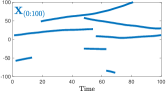
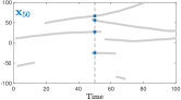
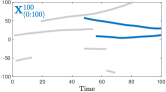
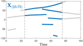
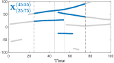
Figure 1: Examples that illustrate Theorem 5. Seven trajectories in the time window $0:100$, in a 1D state space with surveillance area $[-100,\ 100]$. Left to right: set of all trajectories $\mathbf{X}_{0:100}$; corresponding target set at time $50$, $\mathbf{x}_{50}$; corresponding set of current trajectories $\mathbf{X}_{0:100}^{100}$; corresponding set of trajectories in interval $25$ to $75$, $\mathbf{X}_{25:75}$; corresponding set of trajectories in interval $25$ to $75$ alive at some point in the interval $45$ to $55$, $\mathbf{X}_{25:75}^{45:55}$. For the standard point target model, it follows from Theorem 4 that the densities for all these sets of trajectories are pmbm.

After presenting the theorem we give examples for when this may be useful. In what follows, we denote by $\int\mathrm{d}x_{\beta:\varepsilon\backslash b:e}$ the marginalisation of the states in the sequence $x_{\beta:\varepsilon}$ that are not in the time interval $b:e$, where $\beta\leq b\leq e\leq\varepsilon$.

Theorem 5.

Given a posterior pmbm density with parameters as in (28) for the set of all trajectories at time $k$, $\mathbf{X}_{0:k}$, the posterior density for $\mathbf{X}_{\alpha:\gamma}^{\eta:\zeta}$, where $\mathbb{N}_{\eta}^{\zeta}\subseteq\mathbb{N}_{\alpha}^{\gamma}\subseteq\mathbb{N}_{0}^{k}$, is a pmbm density with parameters

$$\tilde{\lambda}^{\rm u}(\cdot),\left\{\left(w^{i,a^{i}},\tilde{r}^{i,a^{i}},\tilde{f}^{i,a^{i}}(\cdot)\right)\right\}_{a\in\mathcal{A},\ i\in\mathbb{T}:\tilde{r}^{i,a^{i}}\neq 0}$$ (43a)

with ppp intensity

$$\tilde{\lambda}^{\rm u}(X)=\sum_{j\in\mathbb{J}^{{\rm u},\eta:\zeta}}\nu^{{\rm u},j}\tilde{f}^{{\rm u},j}(X;\tilde{\theta}^{{\rm u},j}),$$ (43b)

$$\mathbb{J}^{{\rm u},\eta:\zeta}=\left\{j\in\mathbb{J}^{\rm u}:\mathbb{N}_{b^{{\rm u},j}}^{e^{{\rm u},j}}\cap\mathbb{N}_{\eta}^{\zeta}\neq\emptyset\right\},$$ (43c)

$$\tilde{\theta}^{{\rm u},j}=\left(\tilde{b}^{{\rm u},j},\tilde{e}^{{\rm u},j},\tilde{p}^{{\rm u},j}(\cdot)\right),$$ (43d)

$$\tilde{b}^{{\rm u},j}=\max\left(b^{{\rm u},j},\alpha\right),\quad\tilde{e}^{{\rm u},j}=\min\left(e^{{\rm u},j},\gamma\right),$$ (43e)

$$\tilde{p}^{{\rm u},j}(x_{\tilde{b}^{{\rm u},j}:\tilde{e}^{{\rm u},j}})=\int p^{{\rm u},j}(x_{b^{{\rm u},j}:e^{{\rm u},j}})\mathrm{d}x_{b^{{\rm u},j}:e^{{\rm u},j}\backslash\tilde{b}^{{\rm u},j}:\tilde{e}^{{\rm u},j}},$$ (43f)

and Bernoulli parameters

$$\tilde{r}^{i,a^{i}}=r^{i,a^{i}}\sum_{j\in\mathbb{J}^{i,a^{i},\eta:\zeta}}\nu^{i,a^{i},j},$$ (43g)

$$\tilde{f}^{i,a^{i}}(X)=\frac{\sum_{j\in\mathbb{J}^{i,a^{i},\eta:\zeta}}\nu^{i,a^{i},j}\tilde{f}^{i,a^{i},j}(X;\tilde{\theta}^{i,a^{i},j})}{\sum_{j\in\mathbb{J}^{i,a^{i},\eta:\zeta}}\nu^{i,a^{i},j}},$$ (43h)

$$\mathbb{J}^{i,a^{i},\eta:\zeta}=\left\{j\in\mathbb{J}^{i,a^{i}}:\mathbb{N}_{b^{i,a^{i},j}}^{e^{i,a^{i},j}}\cap\mathbb{N}_{\eta}^{\zeta}\neq\emptyset\right\},$$ (43i)

$$\tilde{\theta}^{i,a^{i},j}=\left(\tilde{b}^{i,a^{i},j},\tilde{e}^{i,a^{i},j},\tilde{p}^{i,a^{i},j}(\cdot)\right),$$ (43j)

$$\tilde{b}^{i,a^{i},j}=\max\left(b^{i,a^{i},j},\alpha\right),\tilde{e}^{i,a^{i},j}=\min\left(e^{i,a^{i},j},\gamma\right),$$ (43k)

$$\tilde{p}^{i,a^{i},j}(x_{\tilde{b}^{i,a^{i},j}:\tilde{e}^{i,a^{i},j}})$$ (43l)

$$=\int p^{i,a^{i},j}(x_{b^{i,a^{i},j}:e^{i,a^{i},j}})\mathrm{d}x_{b^{i,a^{i},j}:e^{i,a^{i},j}\backslash\tilde{b}^{i,a^{i},j}:\tilde{e}^{i,a^{i},j}}.$$

Proof.

See Appendix B. ∎

Theorem 5 is understood as follows: from (43c)/(43i) we obtain the densities of the trajectories that are alive in the time interval $\eta:\zeta$. From (43e)/(43k) we get the time of birth and time of most recent state parameters, and from (43f)/(43l) we get the state sequence densities, corresponding to $\alpha:\gamma$.

A few cases of $\alpha:\gamma$ and $\eta:\zeta$ are of particular interest:

• If $\alpha=0$ and $\gamma=\eta=\zeta=k$ then we get $f(\mathbf{X}_{0:k}^{k})$ which is a solution to pf 2.

• If $\alpha=\gamma=\eta=\zeta=k$ then we get $f(\mathbf{X}_{k}^{k})$ which is a solution to pf 3, albeit under a trajectory parametrisation with single time step trajectories $X=(k,k,x_{k})$.

• If $\eta=\alpha$ and $\zeta=\gamma$, then we get $f(\mathbf{X}_{\alpha:\gamma})$, the density of all trajectories in $\alpha:\gamma$.

Some examples of time marginalisation of the set of trajectories $\mathbf{X}_{0:100}$ are illustrated in Figure 1.

VI-B Proof of Theorem 4

Proof.

It follows from Theorem 1 and Theorem 3 that

$$f_{\min(\alpha,\xi):\max(\gamma,\chi)|\xi:\chi}\left(\mathbf{X}_{\min(\alpha,\xi):\max(\gamma,\chi)}\right),$$ (44)

is a pmbm density, where no update (only prediction) is performed for time steps outside the interval $\xi:\chi$. Applying Theorem 5 to (44) concludes the proof. ∎

VI-C Discussion

The proof of Theorem 4 also provides a possible way to compute the density $f_{\alpha:\gamma|\xi:\chi}^{\eta:\zeta}\left(\mathbf{X}_{\alpha:\gamma}^{\eta:\zeta}\right)$: first use the pmbm tracker for all trajectories, and then use time marginalisation to obtain the desired density. Thus, Theorem 4 is not limited to being a theoretical result, it is also practical. However, we note that the pmbm tracker followed by time marginalisation is possibly not the only way to compute the density $f_{\alpha:\gamma|\xi:\chi}^{\eta:\zeta}\left(\mathbf{X}_{\alpha:\gamma}^{\eta:\zeta}\right)$. Compare to the Gaussian result in (2): it is possible to compute the Gaussian density $p(x_{k}|z_{0:K})$ by computing the joint density $p(x_{0:K}|z_{0:K})$ and then marginalizing, however, one can also use forward-backward rts-smoothing, see, e.g., [7]. Design and comparison of alternative implementations to compute the density in Theorem 4 is beyond the scope of this paper.

Using Theorem 5 for $\alpha=\gamma=\eta=\zeta=k$ the relations between the two pmbm trackers, and between the pmbm trackers and the pmbm filter [6], become clear. For example, for the pmbm tracker for all trajectories and the pmbm filter, we have:

$$\small\begin{array}[]{c c c}f_{k|k}(\mathbf{X}_{0:k})\overset{\text{Thm.~{}\ref{th:PredictionAllTrajectories}}}{\rightarrow}&f_{k+1|k}(\mathbf{X}_{0:k+1})\overset{\text{Thm.~{}\ref{th:Update}}}{\rightarrow}&f_{k+1|k+1}(\mathbf{X}_{0:k+1})\\ \\ \big{\downarrow}{\scriptsize\text{Thm.~{}\ref{thm:all_to_trajs_in_a2g_alive_in_e2z}}}&\big{\downarrow}{\scriptsize\text{Thm.~{}\ref{thm:all_to_trajs_in_a2g_alive_in_e2z}}}&\big{\downarrow}{\scriptsize\text{Thm.~{}\ref{thm:all_to_trajs_in_a2g_alive_in_e2z}}}\\ \\ f_{k|k}(\mathbf{x}_{k})\overset{\text{\cite[cite]{[\@@bibref{}{Wil12}{}{}, Thm. 1]}}}{\rightarrow}&f_{k+1|k}(\mathbf{x}_{k+1})\overset{\text{\cite[cite]{[\@@bibref{}{Wil12}{}{}, Thm. 2]}}}{\rightarrow}&f_{k+1|k+1}(\mathbf{x}_{k+1})\end{array}$$

For the pmbm tracker for the current trajectories, similar relations can be established. It follows that marginalising past time steps to obtain a pmbm filter [6] representation, and then predicting and updating, yields the same result as predicting and updating the pmbm tracker, and then marginalising to obtain a pmbm filter representation. Thus, the hypotheses in the pmbm filter may be regarded as implicitly operating on the latest time step of the trajectory hypotheses in the pmbm tracker.

VII Linear Gaussian implementation

Let $\mathcal{X}=\mathbb{R}^{n_{x}}$, $\mathcal{Z}=\mathbb{R}^{n_{z}}$, and let the transition density and measurement model both be linear and Gaussian,

$$\pi^{x}(x|x^{\prime}) =\mathcal{N}\left(x\,;\,Fx^{\prime},Q\right),$$ (45a)

$$\varphi^{z}(z|x) =\mathcal{N}\left(z\,;\,Hx,R\right),$$ (45b)

where $F\in\mathbb{R}^{n_{x}\times n_{x}}$ is a state transition matrix, $H\in\mathbb{R}^{n_{z}\times n_{x}}$ is a measurement matrix, $Q\in\mathbb{S}_{n_{x}}^{++}$ and $R\in\mathbb{S}_{n_{z}}^{++}$ are the covariance matrices of the process noise and measurement noise, respectively, and $\mathbb{S}_{d}^{++}$ denotes the space of positive definite matrices of size $d\times d$.

For linear and Gaussian models (45) we present three alternatives for the state sequence density. In what follows, $m_{k|k}^{[a]}$ and $P_{k|k}^{[a]}$ denote the parts of the mean vector and the covariance matrix for time step $a$, and $P_{k|k}^{[a:b,c:d]}$ denotes the part the covariance matrix with rows for time steps $a$ to $b$ and columns for time steps $c$ to $d$.

VII-A Gaussian moment form

The state sequence density can be expressed on Gaussian moment form, i.e., with mean vector $m_{k|k^{\prime}}$ and covariance matrix $=P_{k|k^{\prime}}$,

$$p_{k|k^{\prime}}(x_{\beta:k}) =\mathcal{N}\left(x_{\beta:k}\ ;\ m_{k|k^{\prime}},P_{k|k^{\prime}}\right),$$ (46)

VII-A1 Prediction

Given the motion model (45) and posterior parameters $m_{k|k}$ and $P_{k|k}$, the predicted parameters are

$$m_{k+1|k} =\begin{bmatrix}m_{k|k}\\ Fm_{k|k}^{[k]}\end{bmatrix},$$ (47a)

$$P_{k+1|k} =\begin{bmatrix}P_{k|k}&P_{k|k}^{[\beta:k,k]}F^{\scriptscriptstyle\mathrm{T}}\\ FP_{k|k}^{[k,\beta:k]}&FP_{k|k}^{[k]}F^{\scriptscriptstyle\mathrm{T}}+Q\end{bmatrix}.$$ (47b)

VII-A2 Update

Given the measurement model (45), predicted parameters $m_{k+1|k}$ and $P_{k+1|k}$, and an associated detection $z$, the posterior parameters are

$$m_{k+1|k+1} =m_{k+1|k}+K(z-Hm_{k+1|k}^{[k]}),$$ (48a)

$$P_{k+1|k+1} =P_{k+1|k}-KHP_{k+1|k}^{[k,\beta:k]},$$ (48b)

$$K =P_{k+1|k}^{[\beta:k,k]}H^{\scriptscriptstyle\mathrm{T}}(HP_{k+1|k}^{[k]}H^{\scriptscriptstyle\mathrm{T}}+R)^{-1}.$$ (48c)

VII-B Gaussian information form

The state sequence density can be expressed on Gaussian information form,

$$p_{k|k^{\prime}}(x_{\beta:k}) =\frac{e^{-\frac{1}{2}y_{k|k^{\prime}}^{T}Y_{k|k^{\prime}}^{-1}y_{k|k^{\prime}}-\frac{1}{2}x_{\beta:k}^{T}Y_{k|k^{\prime}}x_{\beta:k}+y_{k|k^{\prime}}^{T}x_{\beta:k}}}{\sqrt{|2\pi Y_{k|k^{\prime}}^{-1}|}}$$ (49)

with information vector $y_{k|k^{\prime}}$ and information matrix $Y_{k|k^{\prime}}$. The relationship between the moment form and the information form is $y_{k|k^{\prime}}=P_{k|k^{\prime}}^{-1}m_{k|k^{\prime}}$ and $Y_{k|k^{\prime}}=P_{k|k^{\prime}}^{-1}$.

VII-B1 Prediction

Given the motion model (45) and posterior parameters $y_{k|k}$ and $Y_{k|k}$, the predicted parameters are [38, 39, 40]

$$y_{k+1|k} =\begin{bmatrix}\text{\footnotesize$y_{k|k}$}\\ \text{\footnotesize$0_{n_{x}\times 1}$}\end{bmatrix},$$ (50a)

$$Y_{k+1|k} =\begin{bmatrix}\text{\footnotesize$Y_{k|k}^{[\beta:k-1]}$}&\text{\scriptsize$Y_{k|k}^{[\beta:k-1,k]}$}&\text{\footnotesize$0_{(\ell-1)n_{x}\times n_{x}}$}\\ \text{\footnotesize$Y_{k|k}^{[k,\beta:k-1]}$}&\text{\footnotesize$Y_{k|k}^{[k]}+F^{T}Q^{-1}F$}&\text{\footnotesize$-F^{T}Q^{-1}$}\\ \text{\footnotesize$0_{n_{x}\times(\ell-1)n_{x}}$}&\text{\footnotesize$-Q^{-1}F$}&\text{\footnotesize$Q^{-1}$}\end{bmatrix},$$ (50b)

where $0_{m\times n}$ is an $m$ by $n$ all-zero matrix.

VII-B2 Update

Given the measurement model (45), predicted parameters $y_{k+1|k}$ and $Y_{k+1|k}$, and an associated detection $z$, the posterior parameters are [38, 39, 40]

$$y_{k+1|k+1} =y_{k+1|k}+\begin{bmatrix}\text{\footnotesize$0_{(\ell-1)n_{x}\times 1}$}\\ \text{\footnotesize$H^{T}R^{-1}z$}\end{bmatrix},$$ (51a)

$$Y_{k+1|k+1} =Y_{k+1|k}+\begin{bmatrix}\text{\footnotesize$0_{(\ell-1)n_{x}\times(\ell-1)n_{x}}$}&\text{\footnotesize$0_{(\ell-1)n_{x}\times n_{x}}$}\\ \text{\footnotesize$0_{n_{x}\times(\ell-1)n_{x}}$}&\text{\footnotesize$H^{T}R^{-1}H$}\end{bmatrix}.$$ (51b)

VII-C Gaussian L-scan approximation

In [41, Sec. VI.C] it was proposed to represent the state sequence density approximately as a Gaussian,

$$p_{k|k^{\prime}}(x_{\beta:k}) =\mathcal{N}\left(x_{\beta:k}\ ;\ m_{k|k^{\prime}},P_{k|k^{\prime}}\right)$$ (52)

with mean vector $m_{k|k^{\prime}}$ and a covariance matrix with the following structure,

$$P_{k|k^{\prime}}=\mathrm{diag}\left(P_{k|k^{\prime}}^{[\beta]},\ \ldots,P_{k|k^{\prime}}^{[\varepsilon-L]},\ P_{k|k^{\prime}}^{[\varepsilon-L+1:\varepsilon]}\right).$$ (53)

In other words, states before the last $L$ time steps are assumed independent of the most recent $L$ states.

VII-C1 Prediction

Given the motion model (45) and posterior parameters $m_{k|k}$ and $P_{k|k}$, the predicted parameters are

$$m_{k+1|k} =\begin{bmatrix}m_{k|k}\\ Fm_{k|k}^{[k]}\end{bmatrix},$$ (54a)

$$P_{k+1|k} =\mathrm{diag}\left(P_{k|k}^{[\beta]},\ \ldots,\ P_{k|k}^{[k-L]},\ P_{k|k}^{[k-L+1]},\ \Psi\right),$$ (54b)

$$\Psi =\begin{bmatrix}\text{\footnotesize$P_{k|k}^{[k-L+2:k]}$}&\text{\footnotesize$P_{k|k}^{[k-L+2:k,k]}F^{\scriptscriptstyle\mathrm{T}}$}\\ \text{\footnotesize$FP_{k|k}^{[k,k-L+2:k]}$}&\text{\footnotesize$FP_{k|k}^{[k]}F^{\scriptscriptstyle\mathrm{T}}+Q$}\end{bmatrix}.$$ (54c)

VII-C2 Update

Given the measurement model (45), predicted parameters $m_{k+1|k}$ and $P_{k+1|k}$ and an associated detection $z$, the posterior parameters are

$$m_{k+1|k+1}=\begin{bmatrix}m_{k+1|k}^{[\beta:k-L]}\\ m_{k+1|k}^{[k-L+1:k]}+K(z-Hm_{k+1|k}^{[k]})\end{bmatrix},$$ (55a)

$$P_{k+1|k+1}^{[\beta:k-L]}=P_{k+1|k}^{[\beta:k-L]},$$ (55b)

$$P_{k+1|k+1}^{[k-L+1:k]}=P_{k+1|k}^{[k-L+1:k]}-KHP_{k+1|k}^{[k,k-L+1:k]},$$ (55c)

$$K=P_{k+1|k}^{[k-L+1:k,k]}H^{\scriptscriptstyle\mathrm{T}}(HP_{k+1|k}^{[k,k]}H^{\scriptscriptstyle\mathrm{T}}+R)^{-1}.$$ (55d)

VII-D Discussion

In all three predictions, (47), (50) and (54), the mean/covariance, or information vector/matrix, are augmented to account for the additional time step that, following the prediction, is represented by the trajectory. The moment form update (48) and the $L$-scan update (55) affect all states in the state sequence, and the $L$ latest states, respectively. In comparison, the information form update (51) only affects the parts of the information vector and information matrix corresponding to the single most recent state. The number of non-zero elements required by the three different representations are listed in Table I.

TABLE I: Number of non-zero elements

Representation	Mean	Covariance
Moment form	$n_{x}\ell$	$n_{x}^{2}\ell^{2}$
Information form	$n_{z}\left|\mathcal{M}^{k}(i,a^{i})\right|$	$n_{x}^{2}(3\ell-2)$
$L$-scan approximation	$n_{x}\ell$	$n_{x}^{2}\left(L^{2}+\ell-L\right)$

For the information form, a key result is that the bottom left and top right corners of the predicted information matrix (50b) are exactly zero, and that the update (51b) only affects the part of the information matrix that is related to the current state. This means that the information matrix is sparse without approximation, a direct consequence of the Markov property associated with $\pi^{x}(\cdot|\cdot)$. The sparseness has been utilised to formulate accurate and computationally efficient simultaneous localisation and mapping (slam) algorithms, see, e.g., [38, 39, 40].

In theory, when using the Gaussian information form, computing the weights (25b) and (26d), and computing an estimate $\hat{x}_{\hat{\beta}:\hat{\varepsilon}}$, involves the inverse of the information matrix. However, it is not necessary to compute the inverse in practice. Instead, multiplications with the inverse information matrix are solved efficiently as sparse, symmetric, positive-definite, linear system of equations. Utilizing the sparseness does make the computations significantly faster, however, the computational cost inevitably increases with the length of the trajectory. An alternative is to compute, in parallel to the information vector and information matrix, the mean and covariance for the current state, thus making them directly available for computation of the the weights (25b) and (26d). Further discussion about computationally efficient data association, as well as state sequence recovery (both full and partial), for the Gaussian information form can be found in [38, Sec. IV] and [40, Sec. IV-VI].

For the $L$-scan approximation the appropriate choice of $L$ depends on the linear and Gaussian models (45), and how well the cross-covariances $P_{k|k}^{[k,k^{\prime}]}$ can be approximated by all-zero matrices $0_{n_{x}\times n_{x}}$ for time steps $k^{\prime}<k-L$. The simulation study in [41, Sec. VII] showed that the larger $L$ is, the more accurate the resulting tracking filter is, at the price of a computational cost that increases as $L$ increases. One implementation alternative that potentially is computationally cheap and has low memory requirements is a $1$-scan approximation, combined with backwards rts-smoothing, where the backwards smoothing is only performed for selected Bernoulli densities $f_{k|k}^{i,a^{i}}(X)$ when it is deemed necessary, e.g., to perform trajectory estimation [36].

Lastly, the predictions and updates can be generalized to non-linear models, e.g., using linearization; details for the Gaussian information form are found in [38, 39, 40].

VIII Simulation study

In three scenarios we compare three trackers: 1) pmbm tracker for all trajectories, with state sequence density on Gaussian information form, abbreviated pmbm-t-if; 2) pmbm tracker for all trajectories, with $L=1$ scan Gaussian approximation of the state sequence density, abbreviated pmbm-t-$L1$; and 3) a labelled rfs filter, specifically computationally efficient variant of the $\delta$-glmb filter with joint prediction and update [18]. The $\delta$-glmb filter uses an mb birth model instead of a ppp. For a fair comparison, the Gaussian densities in the mb birth were the same as the Gaussian densities in the ppp birth. All compared trackers process the measurements sequentially, one measurement set after another; comparison with trackers that involve multi-scan data association, see, e.g., [42, 43, 24, 36], is outside the scope of this work.

All three trackers used gating with gate probability $0.9999$. In the pmbm trackers, to limit the number of data associations in each update (cf. Theorem 3), analogously to the pmbm filter, see [22, Sec V.C.3], the $M$ best global hypotheses are found using Murty’s algorithm [44]. Pruning was applied to the initial trajectory densities (26f) (threshold $10^{-3}$), as well as to Bernoullis with too small probability of existence (threshold $10^{-5}$). For $\delta$-glmb, we use the standard estimator, see [16]. For the pmbm trackers for all trajectories, we found that setting $r^{\rm e}=1$, cf. Section V-D, yields an estimator that is robust against false trajectories.

Regarding the choice of density representation for the state sequence, cf. Section VII, empirically we found that, for the models and noise covariances simulated in this work, if $L\geq 10$, the tracking results using Gaussian information form and Gaussian $L$-scan approximation are numerically indiscernible.

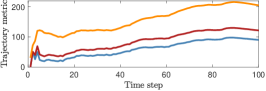
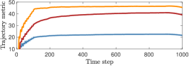
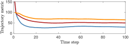
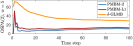
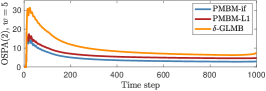
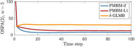
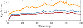
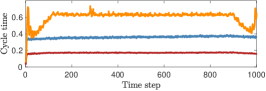
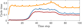
Figure 2: Results from the three simulated scenarios. Left column - scenario 1; middle column - scenario 2; right column - scenario 3.

VIII-A Simulation setup

In all three scenarios a 2D constant velocity motion model, see [45, Sec. III], with Gaussian acceleration standard deviation $\sigma_{v}$ was used. Target measurements were simulated using linear position measurements with Gaussian noise with covariance $R=\mathrm{diag}\left([\sigma_{r}^{2},\ \sigma_{r}^{2}]\right)$. Clutter measurements were simulated uniformly distributed in the surveillance area, with average number of false alarms per time step $\mu^{\rm FA}=\int\lambda^{\rm FA}(z)\mathrm{d}z$. Both $P^{\rm S}$ and $P^{\rm D}$ were set to constant values. The simulation parameters for all three scenarios are listed in Table II, where $K$ denotes the number of time steps in the scenario, and $|\mathbf{X}_{0:K}|$ is the cardinality of the set of all trajectories at the final time step. The birth models and the true trajectories are described in the following.

TABLE II: Simulation parameters

Scenario	$K$	$|\mathbf{X}_{0:K}|$	$\sigma_{v}$	$\sigma_{r}$	$P^{\rm S}$	$P^{\rm D}$	$\mu^{\rm FA}$
1	$100$	$90$	$1$	$1$	0.95	0.99	$100$
2	$1000$	$10$	$1$	$1$	0.99	0.75	$100$
3	$100$	$3$	$0.5$	$10$	0.99	0.98	$1$

VIII-A1 Scenario 1: Many trajectories

The true trajectories were generated by simulating the models in the surveillance area $[-10^{4},10^{4}]\times[-10^{4},10^{4}]$. The trajectories vary in length from $3$ to $83$ time steps, with mean/median length $18.5/14$. The birth density had nine components, with mean positions given by the columns in the following matrix,

$$\begin{bmatrix}-\sqrt{2}&\sqrt{2}&-\sqrt{2}&\sqrt{2}&1&-1&0&0&0\\ -\sqrt{2}&-\sqrt{2}&\sqrt{2}&\sqrt{2}&0&0&1&-1&0\end{bmatrix}\cdot\frac{10^{4}}{2},$$

zero velocity and covariances $\mathrm{diag}\left([500^{2},500^{2},10^{2},10^{2}]\right)$. The expected number of births per time step for each component was set to $1/9$ for all filters.

VIII-A2 Scenario 2: Long trajectories

The times of birth and death were set deterministically to $10,\ 20,\ldots,100$ and $990,\ 980,\ldots,900$, respectively. The trajectories vary in length from $801$ to $981$ time steps. The true trajectories were generated by sampling the initial state from the birth process, and then simulating the motion model in the surveillance area $[-2\times 10^{4},2\times 10^{4}]\times[-2\times 10^{4},2\times 10^{4}]$. The birth density had a single component with mean $[0,0,0,0]^{\scriptscriptstyle\mathrm{T}}$, and covariance $\mathrm{diag}\left([9\cdot 10^{8},9\cdot 10^{8},10^{2},10^{2}]\right)$. The expected number of births per time step was set to $0.01$ for the pmbm trackers, and $0.1$ for the $\delta$-glmb filter. A higher value was used for $\delta$-glmb because with the parameter set to $0.01$ there were too many missed trajectories.

VIII-A3 Scenario 3: Target coalescence

As noted in several previous publications, see, e.g., [6, 23, 22, 24, 35], a large number of spatially separated trajectories, or very long trajectories, is not necessarily the most difficult scenario. Therefore we also simulated a challenging scenario with several targets that start separated, come together at the mid point of the scenario, and then separate again.

The surveillance area was $[-10^{3},10^{3}]\times[-10^{3},10^{3}]$, and the birth density had three components with mean positions given by the columns in the following matrix,

$$\begin{bmatrix}-335&-335&-430\\ 45&-45&0\end{bmatrix},$$

zero velocity and covariances $\mathrm{diag}\left([150^{2},150^{2},10^{2},10^{2}]\right)$. The expected number of births per time step for each component was set to $0.1$ for all filters.

VIII-A4 Performance evaluation

Two performance measures were used: 1) the trajectory metric (tm) [46] with location error cut-off $c=100$, order $p=1$, and switch cost $\gamma=20$; and 2) the ospa(2) metric [47] with location error cut-off $c=100$, orders $p=q=1$, and time window length $w=5$. Both metrics used the Euclidean metric as base metric. tm penalises four types of error: location error (le), missed target error (me), false target error (fe), and switch error (se). ospa(2) penalises two types of errors: location error (le), and a cardinality error (ce). Refer to [46, 47] for metric definitions and further details.

Each metric is computed at each time step, and the result is normalised by the time step. This allows a comparison of how the metrics evolve over time in the scenario, as opposed to, e.g., only computing the metrics at the final time step.

VIII-B Results

Each scenario was simulated 100 times. Monte Carlo average errors, and average cycle times are shown in Figure 2. We see that for all three scenarios, and both metrics, pmbm-t-if outperforms pmbm-t-$L1$, which in turn outperforms $\delta$-glmb. Scenarios 1 and 2 illustrate that the pmbm trackers are not limited to handling a low number of short trajectories, but are capable of handling a high number of long trajectories. Scenario 3 is challenging due to the complex data association when the targets are close for several consecutive time steps.

One interesting difference between the labelled rfs solutions and the pmbm trackers was observed in Scenario 3: the labelled solutions are susceptible to switching that is unrealistic/improbable given the motion model. Two selected example results out of the $100$ Monte Carlo simulations are shown in Figure 3. In the first one all three filters yield reasonable trajectories, however, in the the second example there is unrealistic/improbable switching in the labelled trajectories. This type of switching was not observed in the output from the set of trajectories pmbm filters, which is a direct result of solving mtt using trajectory rfs.

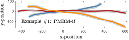
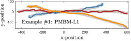
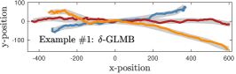
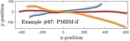
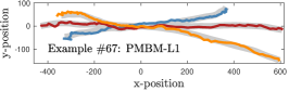
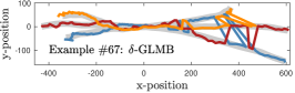
Figure 3: Examples from Scenario 3. #1: similar outputs; #67 $\delta$-glmb results include unrealistic switches, which was not observed for the pmbm trackers.

Lastly, some 1D examples of the estimation of time of birth, and time of most recent state, are given in Appendix C.

IX Conclusions

In this paper we have shown that the set of trajectories pmbm density is conjugate for mtt under assumed standard point target models. We presented two pmbm trackers for the set of target trajectories and evaluated them in a simulation study. Further, we showed that regardless of what time window we consider, for the standard point target model, the exact multi-trajectory density is pmbm, a result analogous to the Gaussian distribution in linear/Gaussian systems.

Appendix A Recursive computation of the probability of most recent state $\varepsilon$

The pmf $P_{k|k}(\varepsilon)$ can also be computed recursively. Let the posterior pmf be $P_{k-1|k-1}(\varepsilon)$, then, given that the association is a missed detection, the predicted and posterior pmfs at time $k$ are

$$P_{k|k-1}(\varepsilon) =\begin{cases}P_{k-1|k-1}(\varepsilon)&\varepsilon<k-1\\ \left(1-P^{\rm S}\right)P_{k-1|k-1}(\varepsilon)&\varepsilon=k-1\\ P^{\rm S}P_{k-1|k-1}(\varepsilon)&\varepsilon=k\end{cases}$$ (56a)

$$P_{k|k}(\varepsilon) =\begin{cases}\frac{P_{k|k-1}(\varepsilon)}{1-P^{\rm D}P_{k|k-1}(k)}&\varepsilon<k-1\\ \frac{\left(1-P^{\rm D}\right)P_{k|k-1}(\varepsilon)}{1-P^{\rm D}P_{k|k-1}(k)}&\varepsilon=k\end{cases}$$ (56b)

Appendix B Proof of Theorem 5

B-A Preliminaries

For trajectories $X\in\mathcal{T}_{0:k}$ we define the function

$$\tau_{\alpha:\gamma}^{\eta:\zeta}(X)= \begin{cases}\left\{\left(b,e,x_{b:e}\right)\right\}&\mathbb{N}_{\beta}^{\varepsilon}\cap\mathbb{N}_{\eta}^{\zeta}\neq\emptyset,\\ \emptyset&\text{otherwise,}\end{cases}$$ (57a)

$$b= \max(\beta,\alpha),\quad e=\min(\varepsilon,\gamma).$$ (57b)

where $0\leq\alpha\leq\eta\leq\zeta\leq\gamma\leq k$. Note that a function corresponding to $\tau_{k:k}^{k:k}(X)$ was defined in [5, Sec. II.A]. For set inputs, like in [5, Sec. II.A], we have

$$\tau_{\alpha:\gamma}^{\eta:\zeta}(\mathbf{X}) =\begin{cases}\bigcup_{X\in\mathbf{X}}\tau_{\alpha:\gamma}^{\eta:\zeta}(X)&\mathbf{X}\neq\emptyset\\ \emptyset&\mathbf{X}=\emptyset\end{cases}$$ (58)

For $\tau_{\alpha:\gamma}^{\eta:\zeta}(\mathbf{X})$ it holds that $\tau_{\alpha:\gamma}^{\eta:\zeta}(\mathbf{X}^{1}\cup\mathbf{X}^{2})=\tau_{\alpha:\gamma}^{\eta:\zeta}(\mathbf{X}^{1})\cup\tau_{\alpha:\gamma}^{\eta:\zeta}(\mathbf{X}^{2})$.

The multi-target Dirac delta is defined as [2, Sec. 11.3.4.3]

$$\delta_{\mathbf{X}^{\prime}}(\mathbf{X})\triangleq\begin{cases}0&|\mathbf{X}|\neq|\mathbf{X}^{\prime}|\\ 1&\mathbf{X}=\mathbf{X}^{\prime}=\emptyset\\ \displaystyle\sum_{\sigma\in\Gamma_{n}}\prod_{i=1}^{n}\delta_{X_{\sigma_{i}}^{\prime}}(X_{i})&\begin{cases}\mathbf{X}=\left\{X_{i}\right\}_{i=1}^{n}\\ \mathbf{X}^{\prime}=\left\{X_{i}^{\prime}\right\}_{i=1}^{n}\end{cases}\end{cases}$$ (59)

From [5, Thm. 11] we know that using the multi-target Dirac delta function and $\tau_{\alpha:\gamma}^{\eta:\zeta}(\mathbf{X})$ we can formulate a transition density from the set $\mathbf{X}_{0:k}$ to the set $\mathbf{X}_{\alpha:\gamma}^{\eta:\zeta}=\tau_{\alpha:\gamma}^{\eta:\zeta}(\mathbf{X}_{0:k})$ as

$$\delta_{\tau_{\alpha:\gamma}^{\eta:\zeta}(\mathbf{X}_{0:k})}\left(\mathbf{X}_{\alpha:\gamma}^{\eta:\zeta}\right).$$ (60)

Lemma 1 shows how this allows us to find the density corresponding to the function $\tau_{\alpha:\gamma}^{\eta:\zeta}(\mathbf{X})$.

Lemma 1.

Suppose $f(\mathbf{X})$ is a pmbm density parameterised as in Section V. Then, if $\mathbf{Y}=\tau_{\alpha:\gamma}^{\eta:\zeta}(\mathbf{X})$, the density for $\mathbf{Y}$ is given by

$$g(\mathbf{Y}) =\int\delta_{\tau_{\alpha:\gamma}^{\eta:\zeta}(\mathbf{X})}(\mathbf{Y})f(\mathbf{X})\delta\mathbf{X}$$ (61a)

$$=\sum_{\begin{subarray}{c}\left(\uplus_{i\in\mathbb{T}}\mathbf{Y}^{i}\right)\uplus\mathbf{Y}^{\rm u}=\mathbf{Y}\end{subarray}}\int\delta_{\tau_{\alpha:\gamma}^{\eta:\zeta}\left(\mathbf{X}^{\rm u}\right)}(\mathbf{Y}^{\rm u})f^{\rm u}(\mathbf{X}^{\rm u})\delta\mathbf{X}^{\rm u}$$

$$\quad\times\sum_{a\in\mathcal{A}}w_{a}\prod_{i\in\mathbb{T}}\int\delta_{\tau_{\alpha:\gamma}^{\eta:\zeta}\left(\mathbf{X}^{i}\right)}(\mathbf{Y}^{i})f^{i,a^{i}}(\mathbf{X}^{i})\delta\mathbf{X}^{i}$$ (61b)

Proof.

Follows from [48, Lem. 2] and [5, Thm. 11]. ∎

Note that in Lemma 1 we have integrals with the transition density and ppp densities and Bernoulli densities. The following Lemmas provide the solutions to these integrals.

Lemma 2.

Let $f(\mathbf{X}_{0:k})$ be a Bernoulli density, with parameters $r$ and $f(X)$. The trajectory rfs density

$$f(\mathbf{X}_{\alpha:\gamma}^{\eta:\zeta})=\int\delta_{\tau_{\alpha:\gamma}^{\eta:\zeta}(\mathbf{X}_{0:k})}(\mathbf{X}_{\alpha:\gamma}^{\eta:\zeta})f(\mathbf{X}_{0:k})\delta\mathbf{X}_{0:k}$$ (62)

is a trajectory Bernoulli density with parameters

$$\tilde{r}= r\Pr\left(\mathbb{N}_{\beta}^{\varepsilon}\cap\mathbb{N}_{\eta}^{\zeta}\neq\emptyset\right)$$ (63a)

$$\tilde{f}(X)= \frac{\displaystyle\sum_{\begin{subarray}{c}\beta,\varepsilon:\\ \mathbb{N}_{\beta}^{\varepsilon}\cap\mathbb{N}_{\eta}^{\zeta}\neq\emptyset\end{subarray}}\int p(x_{\beta:\varepsilon}|\beta,\varepsilon)P(\beta,\varepsilon)\mathrm{d}x_{\beta:\varepsilon\backslash b:e}}{\Pr\left(\mathbb{N}_{\beta}^{\varepsilon}\cap\mathbb{N}_{\eta}^{\zeta}\neq\emptyset\right)}$$ (63b)

where

$$\Pr\left(\mathbb{N}_{\beta}^{\varepsilon}\cap\mathbb{N}_{\eta}^{\zeta}\neq\emptyset\right)=\sum_{\begin{subarray}{c}\beta,\varepsilon:\\ \mathbb{N}_{\beta}^{\varepsilon}\cap\mathbb{N}_{\eta}^{\zeta}\neq\emptyset\end{subarray}}P(\beta,\varepsilon)$$ (64)

Specifically, for

$$f(X)=\sum_{j\in\mathbb{J}}\nu^{j}f^{j}(X;\theta^{j}),$$ (65)

we get

$$\tilde{r}=r\sum_{j\in\mathbb{J}^{\eta:\zeta}}\nu^{j}$$ (66a)

$$\tilde{f}(X)=\frac{\sum_{j\in\mathbb{J}^{\eta:\zeta}}\nu^{j}\tilde{f}^{j}(X;\tilde{\theta}^{j})}{\sum_{j\in\mathbb{J}^{\eta:\zeta}}\nu^{j}}$$ (66b)

$$\tilde{\theta}^{j}=\left(\tilde{b}^{j},\tilde{e}^{j},\tilde{p}^{j}(x_{\tilde{b}^{j}:\tilde{e}^{j}})\right)$$ (66c)

$$\tilde{b}^{j}=\max(b^{j},\alpha),\quad\tilde{e}^{j}=\min(e^{j},\gamma)$$ (66d)

$$\tilde{p}^{j}(x_{\tilde{b}^{j}:\tilde{e}^{j}})=\int p^{j}(x_{b^{j}:e^{j}})\mathrm{d}x_{b^{j}:e^{j}\backslash\tilde{b}^{j}:\tilde{e}^{j}}$$ (66e)

where $\mathbb{J}^{\eta:\zeta}=\left\{j\ :\ \mathbb{N}_{b^{j}}^{e^{j}}\cap\mathbb{N}_{\eta}^{\zeta}\neq\emptyset\right\}$.

Proof.

See (67).

 

$$f \left(\mathbf{X}_{\alpha:\gamma}^{\eta:\zeta}\right)=\int\delta_{\tau_{\alpha:\gamma}^{\eta:\zeta}(\mathbf{X}_{0:k})}\left(\mathbf{X}_{\alpha:\gamma}^{\eta:\zeta}\right)f(\mathbf{X}_{0:k})\delta\mathbf{X}_{0:k}=\delta_{\tau_{\alpha:\gamma}^{\eta:\zeta}(\emptyset)}\left(\mathbf{X}_{\alpha:\gamma}^{\eta:\zeta}\right)(1-r)+\int\delta_{\tau_{\alpha:\gamma}^{\eta:\zeta}(\{X\})}\left(\mathbf{X}_{\alpha:\gamma}^{\eta:\zeta}\right)rf(X)\mathrm{d}X$$ (67a)

$$= \delta_{\emptyset}\left(\mathbf{X}_{\alpha:\gamma}^{\eta:\zeta}\right)(1-r)+\sum_{\begin{subarray}{c}\beta,\varepsilon:\\ \mathbb{N}_{\beta}^{\varepsilon}\cap\mathbb{N}_{\eta}^{\zeta}=\emptyset\end{subarray}}\int\delta_{\emptyset}\left(\mathbf{X}_{\alpha:\gamma}^{\eta:\zeta}\right)rf((x_{\beta:\varepsilon},\beta,\varepsilon))\mathrm{d}x_{\beta:\varepsilon}+\sum_{\begin{subarray}{c}\beta,\varepsilon:\\ \mathbb{N}_{\beta}^{\varepsilon}\cap\mathbb{N}_{\eta}^{\zeta}\neq\emptyset\end{subarray}}\int\delta_{\{\left(b,e,x_{b:e}\right)\}}\left(\mathbf{X}_{\alpha:\gamma}^{\eta:\zeta}\right)rf((x_{\beta:\varepsilon},\beta,\varepsilon))\mathrm{d}x_{\beta:\varepsilon}$$ (67b)

$$= \delta_{\emptyset}\left(\mathbf{X}_{\alpha:\gamma}^{\eta:\zeta}\right)\left(1-r\sum_{\begin{subarray}{c}\beta,\varepsilon:\\ \mathbb{N}_{\beta}^{\varepsilon}\cap\mathbb{N}_{\eta}^{\zeta}\neq\emptyset\end{subarray}}P(\beta,\varepsilon)\right)+r\left(\sum_{\begin{subarray}{c}\beta,\varepsilon:\\ \mathbb{N}_{\beta}^{\varepsilon}\cap\mathbb{N}_{\eta}^{\zeta}\neq\emptyset\end{subarray}}P(\beta,\varepsilon)\right)\frac{\sum_{\begin{subarray}{c}\beta,\varepsilon:\\ \mathbb{N}_{\beta}^{\varepsilon}\cap\mathbb{N}_{\eta}^{\zeta}\neq\emptyset\end{subarray}}\int\delta_{\{\left(b,e,x_{b:e}\right)\}}\left(\mathbf{X}_{\alpha:\gamma}^{\eta:\zeta}\right)p(x_{\beta:\varepsilon}|\beta,\varepsilon)P(\beta,\varepsilon)\mathrm{d}x_{\beta:\varepsilon}}{\sum_{\begin{subarray}{c}\beta,\varepsilon:\\ \mathbb{N}_{\beta}^{\varepsilon}\cap\mathbb{N}_{\eta}^{\zeta}\neq\emptyset\end{subarray}}P(\beta,\varepsilon)}$$ (67c)

$$= \begin{cases}1-r\sum_{\begin{subarray}{c}\beta,\varepsilon:\\ \mathbb{N}_{\beta}^{\varepsilon}\cap\mathbb{N}_{\eta}^{\zeta}\neq\emptyset\end{subarray}}P(\beta,\varepsilon)&\text{if }\mathbf{X}_{\alpha:\gamma}^{\eta:\zeta}=\emptyset\\ r\left(\sum_{\begin{subarray}{c}\beta,\varepsilon:\\ \mathbb{N}_{\beta}^{\varepsilon}\cap\mathbb{N}_{\eta}^{\zeta}\neq\emptyset\end{subarray}}P(\beta,\varepsilon)\right)\frac{\sum_{\begin{subarray}{c}\beta,\varepsilon:\\ \mathbb{N}_{\beta}^{\varepsilon}\cap\mathbb{N}_{\eta}^{\zeta}\neq\emptyset\end{subarray}}\int p(x_{\beta:\varepsilon}|\beta,\varepsilon)\mathrm{d}x_{\beta:\varepsilon\backslash b:e}P(\beta,\varepsilon)}{\sum_{\begin{subarray}{c}\beta,\varepsilon:\\ \mathbb{N}_{\beta}^{\varepsilon}\cap\mathbb{N}_{\eta}^{\zeta}\neq\emptyset\end{subarray}}P(\beta,\varepsilon)}&\text{if }\mathbf{X}_{\alpha:\gamma}^{\eta:\zeta}=\{X\}\end{cases}$$ (67d)

 

∎

Lemma 3.

Let $f(\mathbf{X}_{0:k})$ be a trajectory ppp density, with intensity $\lambda(X)=\mu p(x_{\beta:\varepsilon}|\beta,\varepsilon)P(\beta,\varepsilon)$. The trajectory rfs density

$$f(\mathbf{X}_{\alpha:\gamma}^{\eta:\zeta})=\int\delta_{\tau_{\alpha:\gamma}^{\eta:\zeta}(\mathbf{X}_{0:k})}(\mathbf{X}_{\alpha:\gamma}^{\eta:\zeta})f(\mathbf{X}_{0:k})\delta\mathbf{X}_{0:k}$$ (68)

is a trajectory ppp density with intensity

$$\tilde{\lambda}(X)= \sum_{\begin{subarray}{c}\beta,\varepsilon:\\ \mathbb{N}_{\beta}^{\varepsilon}\cap\mathbb{N}_{\eta}^{\zeta}\neq\emptyset\end{subarray}}\int\mu p(x_{\beta:\varepsilon}|\beta,\varepsilon)P(\beta,\varepsilon)\mathrm{d}x_{\beta:\varepsilon\backslash b:e}$$ (69)

Specifically, for

$$\lambda(X)=\sum_{j\in\mathbb{J}}\nu^{j}f^{j}(X;\theta^{j}),$$ (70)

we get

$$\tilde{\lambda}(X)=\sum_{j\in\mathbb{J}^{\eta:\zeta}}\nu^{j}\tilde{f}^{j}(X;\tilde{\theta}^{j})$$ (71a)

$$\tilde{\theta}^{j}=\left(\tilde{b}^{j},\tilde{e}^{j},\tilde{p}^{j}(x_{\tilde{b}^{j}:\tilde{e}^{j}})\right)$$ (71b)

$$\tilde{b}^{j}=\max(b^{j},\alpha),\quad\tilde{e}^{j}=\min(e^{j},\gamma)$$ (71c)

$$\tilde{p}^{j}(x_{\tilde{b}^{j}:\tilde{e}^{j}})=\int p^{j}(x_{b^{j}:e^{j}})\mathrm{d}x_{b^{j}:e^{j}\backslash\tilde{b}^{j}:\tilde{e}^{j}}$$ (71d)

where $\mathbb{J}^{\eta:\zeta}=\left\{j\ :\ \mathbb{N}_{b^{j}}^{e^{j}}\cap\mathbb{N}_{\eta}^{\zeta}\neq\emptyset\right\}$.

Proof.

From [10, p. 99, Rmk. 12] we know that the ppp $\mathbf{X}_{0:k}$ with intensity $\lambda(X)$ can be divided into two disjoint and independent ppp subsets

$$\mathbf{X}_{0:k}= \mathbf{X}_{0:k}^{\eta:\zeta}\cup\mathbf{X}_{0:k}^{\not\eta:\not\zeta},\quad\mathbf{X}_{0:k}^{\eta:\zeta}\cap\mathbf{X}_{0:k}^{\not\eta:\not\zeta}=\emptyset$$ (72a)

$$\mathbf{X}_{0:k}^{\eta:\zeta}= \left\{X\in\mathbf{X}_{0:k}\ :\ \mathbb{N}_{\beta}^{\varepsilon}\cap\mathbb{N}_{\eta}^{\zeta}\neq\emptyset\right\}$$ (72b)

$$\mathbf{X}_{0:k}^{\not\eta:\not\zeta}= \left\{X\in\mathbf{X}_{0:k}\ :\ \mathbb{N}_{\beta}^{\varepsilon}\cap\mathbb{N}_{\eta}^{\zeta}=\emptyset\right\}$$ (72c)

with ppp intensities

$$\lambda^{\eta:\zeta}(X) =\mathbf{1}_{\mathbb{N}_{\beta}^{\varepsilon}\cap\mathbb{N}_{\eta}^{\zeta}}\lambda(X),$$ (73a)

$$\lambda^{\not\eta:\not\zeta}(X) =\left(1-\mathbf{1}_{\mathbb{N}_{\beta}^{\varepsilon}\cap\mathbb{N}_{\eta}^{\zeta}}\right)\lambda(X),$$ (73b)

where

$$\mathbf{1}_{\mathbb{N}_{\beta}^{\varepsilon}\cap\mathbb{N}_{\eta}^{\zeta}}=\begin{cases}1&\mathbb{N}_{\beta}^{\varepsilon}\cap\mathbb{N}_{\eta}^{\zeta}\neq\emptyset\\ 0&\text{otherwise.}\end{cases}$$ (74)

It is straightforward to verify that $\lambda^{\eta:\zeta}(X)+\lambda^{\not\eta:\not\zeta}(X)=\lambda(X)$. The rest of the proof follows in (75).

 

$$f^{\gamma}(\mathbf{Y})= \int\delta_{\tau_{\alpha:\gamma}^{\eta:\zeta}(\mathbf{X}_{0:k})}(\mathbf{Y})f(\mathbf{X}_{0:k})\delta\mathbf{X}_{0:k}$$ (75a)

$$= \sum_{\begin{subarray}{c}\mathbf{X}_{0:k}^{\eta:\zeta},\mathbf{X}_{0:k}^{\not\eta:\not\zeta}\\ \mathbf{X}_{0:k}^{\eta:\zeta}\uplus\mathbf{X}_{0:k}^{\not\eta:\not\zeta}=\mathbf{Y}\end{subarray}}\int\delta_{\tau_{\alpha:\gamma}^{\eta:\zeta}(\mathbf{X}_{0:k}^{\gamma})}(\mathbf{X}_{0:k}^{\eta:\zeta})f(\mathbf{X}_{0:k}^{\gamma})\delta\mathbf{X}_{0:k}^{\gamma}\int\delta_{\tau_{\alpha:\gamma}^{\eta:\zeta}(\mathbf{X}_{0:k}^{\not\gamma})}(\mathbf{X}_{0:k}^{\not\eta:\not\zeta})f(\mathbf{X}_{0:k}^{\not\gamma})\delta\mathbf{X}_{0:k}^{\not\gamma}$$ (75b)

$$= \int\delta_{\tau_{\alpha:\gamma}^{\eta:\zeta}(\mathbf{X}_{0:k}^{\gamma})}(\mathbf{Y})f(\mathbf{X}_{0:k}^{\gamma})\delta\mathbf{X}_{0:k}^{\gamma}$$ (75c)

$$= \delta_{\emptyset}(\mathbf{Y})e^{-\left\langle\lambda^{\eta:\zeta};1\right\rangle}+\sum_{n=1}^{\infty}\frac{1}{n!}\idotsint\delta_{\tau_{\alpha:\gamma}^{\eta:\zeta}(\{X^{1},\ldots,X^{n}\})}(\mathbf{Y})e^{-\left\langle\lambda^{\eta:\zeta};1\right\rangle}\prod_{i=1}^{n}\lambda^{\eta:\zeta}(X^{i})\mathrm{d}X^{1}\cdots\mathrm{d}X^{n}$$ (75d)

$$= \delta_{\emptyset}(\mathbf{Y})e^{-\left\langle\lambda^{\eta:\zeta};1\right\rangle}+\sum_{n=1}^{\infty}\frac{e^{-\left\langle\lambda^{\eta:\zeta};1\right\rangle}}{n!}\sum_{\begin{subarray}{c}\mathbf{Y}^{1},\ldots,\mathbf{Y}^{n}:\\ \uplus_{i=1}^{n}\mathbf{Y}^{i}=\mathbf{Y}\end{subarray}}\prod_{i=1}^{n}\int\delta_{\tau_{\alpha:\gamma}^{\eta:\zeta}(\{X^{i}\})}(\mathbf{Y}^{i})\lambda^{\eta:\zeta}(X^{i})\mathrm{d}X^{i}$$ (75e)

$$= \delta_{\emptyset}(\mathbf{Y})e^{-\left\langle\lambda^{\eta:\zeta};1\right\rangle}+\sum_{n=1}^{\infty}\frac{e^{-\left\langle\lambda^{\eta:\zeta};1\right\rangle}}{n!}\sum_{\begin{subarray}{c}\mathbf{Y}^{1},\ldots,\mathbf{Y}^{n}:\\ \uplus_{i=1}^{n}\mathbf{Y}^{i}=\mathbf{Y}\end{subarray}}\prod_{i=1}^{n}\sum_{\begin{subarray}{c}\beta,\varepsilon:\\ \mathbb{N}_{\beta}^{\varepsilon}\cap\mathbb{N}_{\eta}^{\zeta}\end{subarray}}\int\delta_{\{X^{i}\}}(\mathbf{Y}^{i})\lambda(X^{i})\mathrm{d}x_{\beta:\varepsilon\backslash b:e}^{i}$$ (75f)

$$= e^{-\left\langle\lambda^{\eta:\zeta};1\right\rangle}\delta_{\emptyset}(\mathbf{Y})+e^{-\left\langle\lambda^{\eta:\zeta};1\right\rangle}\sum_{n=1}^{\infty}\delta_{\{Y^{1},\ldots,Y^{n}\}}(\mathbf{Y})\prod_{i=1}^{n}\sum_{\begin{subarray}{c}\beta,\varepsilon:\\ \mathbb{N}_{\beta}^{\varepsilon}\cap\mathbb{N}_{\eta}^{\zeta}\end{subarray}}\int\delta_{\{X^{i}\}}(\{Y^{i}\})\lambda(X^{i})\mathrm{d}x_{\beta:\varepsilon\backslash b:e}^{i}$$ (75g)

$$= e^{-\mu\sum_{\begin{subarray}{c}\beta,\varepsilon:\mathbb{N}_{\beta}^{\varepsilon}\cap\mathbb{N}_{\eta}^{\zeta}\end{subarray}}P(\beta,\varepsilon)}\prod_{Y\in\mathbf{Y}}\mu p(Y)\sum_{\begin{subarray}{c}\beta,\varepsilon:\mathbb{N}_{\beta}^{\varepsilon}\cap\mathbb{N}_{\eta}^{\zeta}\end{subarray}}P(\beta,\varepsilon)$$ (75h)

 

∎

B-B Proof of Theorem 5

Given a pmbm density $f(\mathbf{X}_{0:k})$ for the set of all trajectories from $0$ to $k$, the density for $\mathbf{X}_{\alpha:\gamma}^{\eta:\zeta}$, where $0\leq\alpha\leq\eta\leq\zeta\leq\gamma\leq k$, is given by [5, Thm. 11]

$$f(\mathbf{X}_{\alpha:\gamma}^{\eta:\zeta})=\int\delta_{\tau_{\alpha:\gamma}^{\eta:\zeta}(\mathbf{X}_{0:k})}(\mathbf{X}_{\alpha:\gamma}^{\eta:\zeta})f(\mathbf{X}_{0:k})\delta\mathbf{X}_{0:k}$$ (76)

Theorem 5 then follows from Lemmas 1, 2 and 3.

Appendix C Illustrations of $\beta$ and $\varepsilon$

Figure 4 and Figure 5 illustrate how the pmbm trackers compute pmfs for $\beta$ and $\varepsilon$. In Figure 4 we see how the pmf for $\beta$ changes as more detections are associated. In Figure 5 we see how, when only misdetections are associated, the map estimate of $\varepsilon$ eventually becomes the time of last associated measurement.

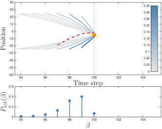
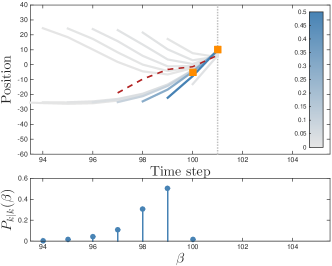
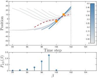
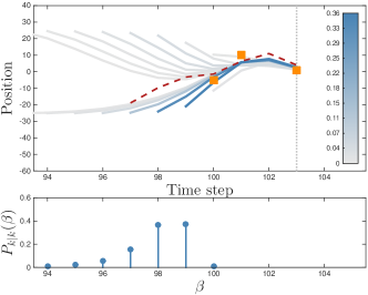
Figure 4: Birth ppp intensity with two components with mean $-25$ and $25$, and standard deviation $5$. Dashed red: true trajectory. Orange squares: measurements. Dotted gray vertical: current time step $k$. Blue solid: expected state sequence hypotheses, color corresponds to probability of hypothesis (see colorbar). First measurement associated at $k=100$; note how both pmf $P_{k|k}(\beta)$ and expected state sequences change as more measurements are associated.

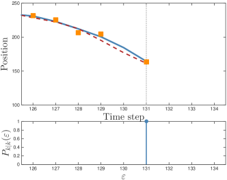
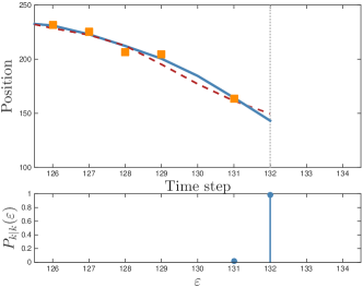
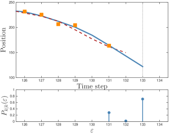
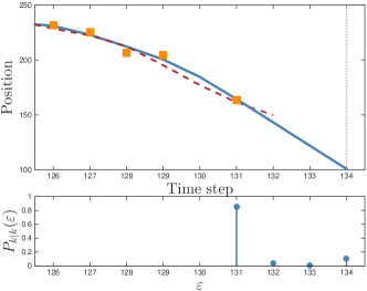
Figure 5: At $k=131$ a detection is associated to a Bernoulli component. After $k=131$, only misdetections are associated. Dashed red: true trajectory. Orange squares: associated measurements. Dotted gray vertical: current time step $k$. Blue solid: state sequence. Pmf $P_{k|k}(\varepsilon)$ changes as time since last association increases.

References

• [1] Y. Bar-Shalom, P. K. Willett, and X. Tian, Tracking and Data Fusion: A Handbook of Algorithms.   YBS Publishing, 2011.
• [2] R. P. S. Mahler, Statistical Multisource-Multitarget Information Fusion.   Norwood, MA: Artech House, 2007.
• [3] K. Granström, M. Baum, and S. Reuter, “Extended Object Tracking: Introduction, Overview and Applications,” Jour. Adv. Inform. Fusion, vol. 12, no. 2, pp. 139–174, Dec. 2017.
• [4] L. Svensson and M. Morelande, “Target tracking based on sets of trajectories,” in Proc. Int. Conf. Inform. Fusion, Salamanca, Spain, Jul. 2014.
• [5] A. F. García-Fernández, L. Svensson, and M. R. Morelande, “Multiple target tracking based on sets of trajectories,” IEEE Trans. Aerosp. Electron. Syst., DOI: 10.1109/TAES.2019.2921210.
• [6] J. L. Williams, “Marginal multi-Bernoulli filters: RFS derivation of MHT, JIPDA and association-based MeMBer,” IEEE Trans. Aerosp. Electron. Syst., vol. 51, no. 3, July 2015.
• [7] S. Särkkä, Bayesian Filtering and Smoothing.   Cambridge University Press, 2013.
• [8] S. Coraluppi and C. A. Carthel, “If a tree falls in the woods, it does make a sound: multiple-hypothesis tracking with undetected target births,” IEEE Trans. Aerosp. Electron. Syst., vol. 50, no. 3, pp. 2379–2388, July 2014.
• [9] D. B. Reid, “An algorithm for tracking multiple targets,” IEEE Trans. Automatic Control, vol. AC-24, no. 6, pp. 843–854, December 1979.
• [10] R. Mahler, Advances in Multisource-Multitarget Information Fusion.   Norwood, MA, USA: Artech House, 2014.
• [11] S. Mori, C.-Y. Chong, E. Tse, and R. Wishner, “Tracking and classifying multiple targets without a priori identification,” IEEE Trans. Automatic Control, vol. 31, no. 5, pp. 401–409, May 1986.
• [12] E. Brekke and M. Chitre, “Relationship between finite set statistics and the multiple hypothesis tracker,” IEEE Transactions on Aerospace and Electronic Systems, vol. 54, no. 4, pp. 1902–1917, Aug. 2018.
• [13] R. Mahler, “Multitarget Bayes filtering via first-order multi target moments,” IEEE Trans. Aerosp. Electron. Syst., vol. 39, no. 4, pp. 1152–1178, Oct. 2003.
• [14] A. F. Garcia-Fernandez, J. Grajal, and M. R. Morelande, “Two-layer particle filter for multiple target detection and tracking,” IEEE Trans. Aerosp. Electron. Syst., vol. 49, no. 3, pp. 1569–1588, Jul. 2013.
• [15] E. H. Aoki, P. K. Mandal, L. Svensson, Y. Boers, and A. Bagchi, “Labeling uncertainty in multitarget tracking,” IEEE Trans. Aerosp. Electron. Syst., vol. 52, no. 3, pp. 1006–1020, Jun. 2016.
• [16] B.-T. Vo and B.-N. Vo, “Labeled random finite sets and multi-object conjugate priors,” IEEE Trans. Signal Process., vol. 61, no. 13, pp. 3460–3475, 2013.
• [17] B.-T. Vo, B.-N. Vo, and D. Phung, “Labeled random finite sets and the Bayes multi-target tracking filter,” IEEE Trans. Signal Process., vol. 62, no. 24, pp. 6554–6567, Dec. 2014.
• [18] B. N. Vo, B. T. Vo, and H. G. Hoang, “An efficient implementation of the generalized labeled multi-Bernoulli filter,” IEEE Trans. Signal Process., vol. 65, no. 8, pp. 1975–1987, Apr. 2017.
• [19] K. Panta, D. Clark, and B.-N. Vo, “Data association and track management for the Gaussian mixture probability hypothesis density filter,” IEEE Trans. Aerosp. Electron. Syst., vol. 45, no. 3, pp. 1003–1016, Jul. 2009.
• [20] J. Houssineau and D. E. Clark, “Multitarget filtering with linearized complexity,” IEEE Trans. Signal Process., vol. 66, no. 18, pp. 4957–4970, Sep. 2018.
• [21] K. Granström, M. Fatemi, and L. Svensson, “Poisson multi-Bernoulli conjugate prior for multiple extended object filtering,” IEEE Trans. Aerosp. Electron. Syst., DOI 10.1109/TAES.2019.2920220.
• [22] A. F. García-Fernández, J. Williams, K. Granström, and L. Svensson, “Poisson multi-Bernoulli mixture filter: direct derivation and implementation,” IEEE Trans. Aerosp. Electron. Syst., vol. 54, no. 4, Aug. 2018.
• [23] Y. Xia, K. Granström, L. Svensson, and A. F. García-Fernández, “Performance evaluation of multi-Bernoulli conjugate priors for multi-target filtering,” in Proc. Int. Conf. Inform. Fusion, Xi’an, China, Jul. 2017.
• [24] ——, “An implementation of the Poisson multi-Bernoulli mixture trajectory filter via dual decomposition,” in Proc. Int. Conf. Inform. Fusion, Cambridge, UK, Jul. 2018.
• [25] K. Granström, M. Fatemi, and L. Svensson, “Gamma Gaussian inverse-Wishart Poisson multi-Bernoulli Filter for Extended Target Tracking,” in Proc. Int. Conf. Inform. Fusion, Heidelberg, Germany, Jul. 2016.
• [26] Y. Xia, K. Granström, L. Svensson, A. F. García-Fernández, and J. L. Williams, “Extended target Poisson multi-Bernoulli mixture trackers based on sets of trajectories,” in Proc. Int. Conf. Inform. Fusion, Ottawa, Canada, Jul. 2019.
• [27] K. Granström, S. Reuter, M. Fatemi, and L. Svensson, “Pedestrian tracking using velodyne data - stochastic optimization for extended object tracking,” in Proc. IEEE Intel. Veh. Symp., Redondo Beach, CA, USA, Jun. 2017, pp. 39–46.
• [28] L. Cament, M. Adams, J. Correa, and C. Perez, “The $\delta$-generalized multi-Bernoulli Poisson filter in a multi-sensor application,” in Int. Conf. Cont. Autom. Inform. Sci. (ICCAIS), Oct. 2017, pp. 32–37.
• [29] L. Cament, M. Adams, and J. Correa, “A multi-sensor, Gibbs sampled, implementation of the multi-Bernoulli Poisson filter,” in Proc. Int. Conf. Inform. Fusion, Cambridge, UK, Jul. 2018, pp. 2580–2587.
• [30] K. Granström, L. Svensson, S. Reuter, Y. Xia, and M. Fatemi, “Likelihood-based data association for extended object tracking using sampling methods,” IEEE Trans. Intel. Veh., vol. 3, no. 1, Mar. 2018.
• [31] S. Scheidegger, J. Benjaminsson, E. Rosenberg, A. Krishnan, and K. Granström, “Mono-camera 3D multi-object tracking using deep learning detections and PMBM filtering,” in Proc. IEEE Intel. Veh. Symp., Changshu, Suzhou, China, Jun. 2018.
• [32] M. Motro and J. Ghosh, “Measurement-wise occlusion in multi-object tracking,” in Proc. Int. Conf. Inform. Fusion, Jul. 2018, pp. 2384–2391.
• [33] M. Fatemi, K. Granström, L. Svensson, F. Ruiz, and L. Hammarstrand, “Poisson multi-Bernoulli mapping using Gibbs sampling,” IEEE Trans. Signal Process., vol. 65, no. 11, pp. 2814–2827, Jun. 2017.
• [34] M. Fröhle, C. Lindberg, K. Granström, and H. Wymeersch, “Multisensor Poisson multi-Bernoulli filter for joint target-sensor state tracking,” IEEE Trans. Intel. Veh., DOI 10.1109/TIV.2019.2938093.
• [35] K. Granström, L. Svensson, Y. Xia, J. Williams, and A. F. García-Fernández, “Poisson multi-Bernoulli mixture trackers: Continuity through random finite sets of trajectories,” in Proc. Int. Conf. Inform. Fusion, Cambridge, UK, Jul. 2018.
• [36] Y. Xia, K. Granström, L. Svensson, A. F. García-Fernández, and J. L. Williams, “Multi-scan implementation of the trajectory Poisson multi-Bernoulli mixture filter,” Jour. Adv. Inform. Fusion, Accepted, pre-print available: https://arxiv.org/abs/1912.01748.
• [37] A. F. García-Fernández, Y. Xia, K. Granström, L. Svensson, and J. L. Williams, “Gaussian implementation of the multi-Bernoulli mixture filter,” in Proc. Int. Conf. Inform. Fusion, Ottawa, Canada, Jul. 2019.
• [38] R. M. Eustice, H. Singh, and J. J. Leonard, “Exactly sparse delayed-state filters for view-based SLAM,” IEEE Trans. Robot., vol. 22, no. 6, pp. 1100–1114, 2006.
• [39] M. R. Walter, R. M. Eustice, and J. J. Leonard, “Exactly sparse extended information filters for feature-based SLAM,” International Journal of Robotics Research, vol. 26, no. 4, pp. 335–359, Apr. 2007.
• [40] I. Mahon, S. B. Williams, O. Pizarro, and M. Johnson-Roberson, “Efficient view-based SLAM using visual loop closures,” IEEE Trans. Robot., vol. 24, no. 5, pp. 1002–1014, Oct. 2008.
• [41] A. F. García-Fernández and L. Svensson, “Trajectory PHD and CPHD filters,” IEEE Trans. Signal Process., vol. 67, no. 22, pp. 5702–5714, Nov. 2019.
• [42] R. A. Lau and J. L. Williams, “Multidimensional assignment by dual decomposition,” in Int. Conf. Intel. Sensors, Sensor Netw. and Inform. Proc. (ISSNIP), Dec. 2011, pp. 437–442.
• [43] B. Vo and B. Vo, “A multi-scan labeled random finite set model for multi-object state estimation,” IEEE Trans. Signal Process., vol. 67, no. 19, pp. 4948–4963, Oct. 2019.
• [44] K. Murty, “An algorithm for ranking all the assignments in order of increasing cost,” Operations Research, vol. 16, no. 3, pp. 682–687, 1968.
• [45] X. Rong-Li and V. Jilkov, “Survey of maneuvering target tracking: Part I. Dynamic models,” IEEE Trans. Aerosp. Electron. Syst., vol. 39, no. 4, pp. 1333–1364, Oct. 2003.
• [46] A. S. Rahmathullah, Á. F. García-Fernández, and L. Svensson, “A metric on the space of finite sets of trajectories for evaluation of multi-target tracking algorithms,” arXiv pre-print, 2016. [Online]. Available: arxiv.org/abs/1605.01177
• [47] M. Beard, B. T. Vo, and B. Vo, “OSPA(2): Using the OSPA metric to evaluate multi-target tracking performance,” in Int. Conf. Control, Autom. Inform. Sci. (ICCAIS), Oct. 2017, pp. 86–91.
• [48] J. Williams, “An efficient, variational approximation of the best fitting multi-Bernoulli filter,” IEEE Trans. Signal Process., vol. 63, no. 1, pp. 258–273, Jan. 2015.