Flavor physics and CP violation

OUTLINE

1. Introduction: Why $N_{q}=N_{l}$ and why we are sure that $N_{g}=3$.

2. Cabibbo-Kobayashi-Maskawa (CKM) matrix, unitarity triangles.

3. CP, CP violation.

4. $M^{0}-\bar{M}^{0}$ mixing, CPV in mixing.

5. Neutral kaons: mixing ($\Delta m_{LS}$) and CPV in mixing ($\tilde{\varepsilon}$).

6. Direct CPV.

7. Constraints on the unitarity triangle.

8. CPV in $B^{0}-\bar{B}^{0}$ mixing.

9. CPV in interference of mixing and decays, $B^{0}(\bar{B}^{0})\to J/\Psi K$, angle $\beta$.

10. What is the probability of $\Upsilon(4S)\rightarrow B_{d}^{0}\bar{B}_{d}^{0}\to J/\Psi K_{S}\;J/\Psi K_{S}$ decay?

11. CPV in $b\to sg\to ss\bar{s}$ transition: penguin domination.

12. $B_{s}(\bar{B}_{s})\to J/\Psi\phi,\phi_{s}$.

13. Angles $\alpha$ and $\gamma$.

14. CKM fit.

15. Perspectives: $K\longrightarrow\pi\nu\nu$, Belle II, LHC.

0.1 Introduction

0.1.1 Fundamental particles and Periodic Table

One of the main problems for particle physics in the 21st century is why there are 3 quark-lepton generations and what explains fermion properties. This is a modern version of I.Rabi question which he asked in response to the news that a recently discovered muon is not a hadron: “Who ordered that?”

Dmitry Mendeleev, professor of St. Petersburg University, discovered his Periodic Table in 1869, just 150 years ago. He put there 63 existing elements and predicted 4 new elements. This 19th century discovery was explained by Quantum Mechanics in the beginning of the 20th century. Let us hope that an explanation of the Table of Elementary Particles in general and the solution of a flavor problem in particular will be found in this century. There is much in common with the Periodic Table: $W,Z,H$ with their masses were predicted as well. The central question is: what is an analog of Quantum Mechanics?

0.1.2 More generations?

After the discovery of the third generation the speculations on the 4th generation were very popular. Why only 3?

However for invisible Z boson width we have:

$$\Gamma_{Z\to ff}=\frac{G_{F}M_{Z}^{3}}{6\sqrt{2}\pi}[(g_{V}^{f})^{2}+(g_{A}^{f})^{2}]=332[(g_{V}^{f})^{2}+(g_{A}^{f})^{2}]\;\mbox{\rm MeV}.\;\;$$ (1)

And taking into account $\nu_{e},\nu_{\mu}$ and $\nu_{\tau}$ we obtain:

$$\Gamma_{Z\to\nu\nu}^{\mbox{theor}}=3\cdot 332[\frac{1}{4}+\frac{1}{4}]=498\;\mbox{\rm MeV}\;\;,$$ (2)

$$\Gamma_{inv}^{\mbox{exp}}=499\pm 1.5\;\mbox{\rm MeV}\;\;.$$ (3)

Thus $\nu_{4}$ is not allowed - so, there is no 4th generation.

BUT: what if $m(\nu_{4})>M_{Z}/2$?

In H production at LHC the following diagram dominates:

and for $2m_{t}>>M_{H}$ the corresponding amplitude does not depend on $m_{t}$.

In case of the 4th generation $T-$ and $B-$ quarks contribute as well, so the amplitude triples and the cross section of $H$ production at LHC becomes 9 times larger than in SM, which is definitely excluded by experimental data.

Problem 1

At LHC the values of signal strength $\mu_{f}\equiv\sigma(pp\longrightarrow H+X)*Br(H\longrightarrow f)/()_{SM}$ are measured. What will the change in $\mu_{f}$ be in case of the fourth generation?

0.1.3 Why $N_{q}=N_{l}$?

$N_{q}=N_{l}$ in order to compensate chiral anomalies, which violate conservation of gauge axial currents, making theory nonrenormalizable.

The case of QED:

Unlike QED, $SU(2)_{L}\times U(1)$ gauge invariant Standard Model (SM) deals with Weyl fermions. Thus the gauge bosons $A_{i}$ and $B$ interact with axial currents. In each generation the quarkonic and leptonic $A_{i}^{2}B$ and $B^{3}$ triangles compensate each other, that is why $N_{q}$ should be equal to $N_{l}$.

Problem 2

Prove that the quarkonic triangles cancel the leptonic ones when $Q_{e}=-Q_{p}$ (so hydrogen atoms are neutral) and $Q_{n}=Q_{\nu}=0$ (thus neutrino and neutron are neutral).

0.2 Cabibbo-Kobayashi-Maskawa (CKM) matrix, unitarity triangles

0.2.1 The CKM matrix - where from?

In constructing the Standard Model Lagrangian the basic ingredients are:

1. gauge group,

2. particle content,

3. renormalizability of the theory.

There is no such a building block in the Standard Model as CKM matrix in charged current quark interactions.

This is the SM lagrangian:

$${\cal L}_{\rm SM}=-\frac{1}{2}{\rm tr}G_{\mu\nu}^{2}-\frac{1}{2}{\rm tr}A_{\mu\nu}^{2}-\frac{1}{4}B_{\mu\nu}^{2}+|D_{\mu}H|^{2}-\frac{\lambda^{2}}{2}[H^{+}H-\eta^{2}/2]^{2}+$$

$$+\bar{Q}_{L}^{i}\hat{D}Q_{L}^{i}+\bar{u}_{R}^{i}\hat{D}u_{R}^{i}+\bar{d}_{R}^{i}\hat{D}d_{R}^{i}+\bar{L}_{L}^{i}\hat{D}L_{L}^{i}+\bar{l}_{R}^{i}\hat{D}l_{R}^{i}+\bar{N}_{R}^{i}\hat{\partial}N_{R}^{i}+$$ (4)

$$+\left[f_{ik}^{(u)}\bar{Q}_{L}^{i}u_{R}^{k}H+f_{ik}^{(d)}\bar{Q}_{L}^{i}d_{R}^{k}\tilde{H}+f_{ik}^{(\nu)}\bar{L}_{L}^{i}N_{R}^{k}H+f_{ik}^{(l)}\bar{L}_{L}^{i}l_{R}^{k}\tilde{H}+M_{ik}N_{R}^{i}C^{+}N_{R}^{k}+c.c.\right],$$

$$\hat{D}\equiv D_{\mu}\gamma_{\mu}\;,\;\;D_{\mu}=\partial_{\mu}-ig_{s}G_{\mu}^{i}\lambda_{i}/2-igA_{\mu}^{i}\sigma_{i}/2-ig^{\prime}B_{\mu}Y/2,$$ (5)

where we suppose that neutrinos get masses by the see-saw mechanism.

CKM matrix originates from Higgs field interactions with quarks.

(All quark fields are primed: $Q_{L}\rightarrow Q_{L}^{{}^{\prime}},u_{R}\rightarrow u_{R}^{{}^{\prime}},...$)

0.2.2 CKM matrix originates from Higgs field interactions with quarks.

The piece of the Lagrangian from which the up quarks get their masses looks like:

$$\Delta{\cal L}_{\rm up}=f_{ik}^{(u)}\bar{Q}_{L}^{i^{\prime}}u_{R}^{k^{\prime}}H+{\rm c.c.}\;,\;\;i,k=1,2,3\;\;,$$ (6)

where

$$Q_{L}^{1^{\prime}}=\left(\begin{array}[]{cc}u^{\prime}\\ d^{\prime}\\ \end{array}\right)_{L}\;,\;\;Q_{L}^{2^{\prime}}=\left(\begin{array}[]{cc}c^{\prime}\\ s^{\prime}\\ \end{array}\right)_{L}\;,\;\;Q_{L}^{3^{\prime}}=\left(\begin{array}[]{cc}t^{\prime}\\ b^{\prime}\\ \end{array}\right)_{L}\;\;;$$ (7)

$$u_{R}^{1^{\prime}}=u_{R}^{\prime}\;,\;\;u_{R}^{2^{\prime}}=c_{R}^{\prime}\;,\;\;u_{R}^{3^{\prime}}=t_{R}^{\prime}$$ (8)

and $H$ is the higgs doublet:

$$H=\left(\begin{array}[]{cc}H^{0}\\ H^{-}\end{array}\right).$$ (9)

The piece of the Lagrangian which is responsible for the down quark masses looks the same way:

$$\Delta{\cal L}_{\rm down}=f_{ik}^{(d)}\bar{Q}_{L}^{i^{\prime}}d_{R}^{k^{\prime}}\tilde{H}+{\rm c.c.}\;,$$ (10)

where

$$d_{R}^{1^{\prime}}=d_{R}^{\prime}\;,\;\;d_{R}^{2^{\prime}}=s_{R}^{\prime}\;,\;\;d_{R}^{3^{\prime}}=b_{R}^{\prime}\;\;{\rm and}\;\;\tilde{H}_{a}=\varepsilon_{ab}H_{b}^{*}\;,$$ (11)

$$\varepsilon_{ab}=\left(\begin{array}[]{rl}0&1\\ -1&0\end{array}\right)\;.$$ (12)

After $SU(2)\times U(1)$ symmetry breaking by the Higgs field expectation value ${<H^{0}>=v}$, two mass matrices emerge:

$$M_{\rm up}^{ik}\bar{u}_{L}^{i^{\prime}}u_{R}^{k^{\prime}}+M_{\rm down}^{ik}\bar{d}_{L}^{i^{\prime}}d_{R}^{k^{\prime}}+c.c.$$ (13)

The matrices $M_{\rm up}$ and $M_{\rm down}$ are arbitrary 3$\times$3 matrices; their matrix elements are complex numbers. According to the very useful theorem, an arbitrary matrix can be written as a product of the hermitian and unitary matrices:

$$M=UH\;,\;\;{\rm where}\;\;H=H^{+}\;,\;\;{\rm and}\;\;UU^{+}=1\;\;,$$ (14)

(do not mix the hermitian matrix $H$ with the Higgs field!) which is analogous to the following representation of an arbitrary complex number:

$$a=e^{i\phi}|a|\;\;.$$ (15)

Matrix $M$ can be diagonalized by 2 different unitary matrices acting from left and right:

$$U_{L}MU_{R}^{+}=M_{\rm diag}=\left(\begin{array}[]{ccc}m_{u}&&0\\ &m_{c}&\\ 0&&m_{t}\end{array}\right)\;\;,$$ (16)

where $m_{i}$ are the real numbers (if matrix $M$ is hermitian ($M=M^{+}$) then we will get $U_{L}=U_{R}$, the case of hamiltonian in QM). Having these formulas in mind, let us rewrite the up-quarks mass term:

$$\bar{u}_{L}^{i^{\prime}}M_{ik}u_{R}^{k^{\prime}}+c.c.\equiv\bar{u}_{L}^{\prime}U_{L}^{+}U_{L}MU_{R}^{+}U_{R}u_{R}^{\prime}+c.c.=\bar{u}_{L}M_{\rm diag}u_{R}+c.c.=\bar{u}M_{\rm diag}u\;\;,$$ (17)

where we introduce the fields $u_{L}$ and $u_{R}$ according to the following formulas:

$$u_{L}=U_{L}u_{L}^{\prime}\;,\;\;u_{R}=U_{R}u_{R}^{\prime}\;\;.$$ (18)

Applying the same procedure to matrix $M_{\rm down}$ we observe that it becomes diagonal as well in the rotated basis:

$$d_{L}=D_{L}d_{L}^{\prime}\;,\;\;d_{R}=D_{R}d_{R}^{\prime}\;\;.$$ (19)

Thus we start from the primed quark fields and get that they should be rotated by 4 unitary matrices $U_{L}$, $U_{R}$, $D_{L}$ and $D_{R}$ in order to obtain unprimed fields with diagonal masses.

Since kinetic energies and interactions with the vector fields $A_{\mu}^{3}$, $B_{\mu}$ and gluons are proportional to the unit matrix, these terms remain diagonal in a new unprimed basis. The only term in the SM Lagrangian where matrices $U$ and $D$ show up is charged current interactions with the emission of $W$-boson:

$$\Delta{\cal L}=gW_{\mu}^{+}\bar{u}_{L}^{\prime}\gamma_{\mu}d_{L}^{\prime}=gW_{\mu}^{+}\bar{u}_{L}\gamma_{\mu}U_{L}D_{L}^{+}d_{L}\;\;,$$ (20)

and the unitary matrix $V\equiv U_{L}D_{L}^{+}$ is called Cabibbo-Kobayashi-Maskawa (CKM) quark mixing matrix.

0.2.3 Parametrization of the CKM matrix: angles, phases, unitarity triangles

$n\times n$ unitary matrix has $n^{2}/2$ complex or $n^{2}$ real parameters. The orthogonal $n\times n$ matrix is specified by $n(n-1)/2$ angles (3 Euler angles in case of $O(3)$). That is why the parameters of the unitary matrix are divided between phases and angles according to the following relation:

$$\begin{array}[]{cccc}n^{2}=&{\frac{n(n-1)}{2}}&+&\frac{n(n+1)}{2}\;\;.\\ &&&\\ &{\rm angles}&&{\rm phases}\end{array}$$ (21)

Are all these phases physical observables or, in other words, can they be measured experimentally?

The answer is “no” since we can perform phase rotations of quark fields ($u_{L}\to e^{i\zeta}u_{L}$, $d_{L}\to e^{i\xi}d_{L}$ …) removing in this way $2n-1$ phases of the CKM matrix. The number of unphysical phases equals the number of up and down quark fields minus one. The simultaneous rotation of all up-quarks on one and the same phase multiplies all the matrix elements of matrix $V$ by (minus) this phase. The rotation of all down-quark fields on one and the same phase acts on $V$ in the same way. That is why the number of the “unremovable” phases of matrix $V$ is decreased by the number of possible rotations of up and down quarks minus one.

Finally for the number of observable phases we get:

$$\frac{n(n+1)}{2}-(2n-1)=\frac{(n-1)(n-2)}{2}\;\;.$$ (22)

As you see, for the first time one observable phase arrives in the case of 3 quark-lepton generations.

0.2.4 A bit of history

Introduced in 1963 by Cabibbo angle $\theta_{c}$ [2] in a modern language mixes $d$- and $s$-quarks in the expression for the charged quark current:

$$J_{\mu}^{+}=\bar{u}\gamma_{\mu}(1+\gamma_{5})[d\cos\theta_{c}+s\sin\theta_{c}]\;\;.$$ (23)

In this way he related the suppression of the strange particles weak decays to the smallness of angle $\theta_{c}$, $\sin^{2}\theta_{c}\approx 0.05$. In order to explain the suppression of $K^{0}-\bar{K}^{0}$ transition the GIM mechanism (and c-quark) was suggested in 1970 [4]. After the discovery of a $J/\Psi$-meson made from ($c\bar{c}$) quarks in 1974 it was confirmed that 2 quark-lepton generations exist. The mixing of two quark generations is described by the unitary 2$\times$2 matrix parametrised by one angle and zero observable phases. This angle is Cabibbo angle.

However, even before the $c$-quark discovery in 1973 Kobayashi and Maskawa noticed that one of the several ways to implement CP-violation in the Standard Model is to postulate the existence of 3 quark-lepton generations since for the first time the observable phase shows up for $n=3$ [5]. At that time CPV was known only in neutral $K$-meson decays and to test KM mechanism one needed other systems. Almost 30 years after KM model had been suggested it was confirmed in $B$-meson decays.

Here is the CKM matrix

$$\overline{(uct)_{L}}\left(\begin{array}[]{lll}V_{ud}&V_{us}&V_{ub}\\ V_{cd}&V_{cs}&V_{cb}\\ V_{td}&V_{ts}&V_{tb}\end{array}\right)\left(\begin{array}[]{c}d\\ s\\ b\end{array}\right)_{L},\;\;$$ (24)

and it’s standard parametrization looks like:

$$V=R_{23}\times R_{13}\times R_{12}\;\;,$$ (25)

$$R_{23}=\left(\begin{array}[]{ccc}1&0&0\\ 0&c_{23}&s_{23}\\ 0&-s_{23}&c_{23}\end{array}\right),\;R_{13}=\left(\begin{array}[]{ccc}c_{13}&0&s_{13}e^{-i\delta}\\ 0&1&0\\ -s_{13}e^{i\delta}&0&c_{13}\end{array}\right),\;R_{12}=\left(\begin{array}[]{ccc}c_{12}&s_{12}&0\\ -s_{12}&c_{12}&0\\ 0&0&1\end{array}\right),$$ (26)

and, finally:

$$V=\left(\begin{array}[]{ccc}c_{13}c_{12}&c_{13}s_{12}&s_{13}e^{-i\delta}\\ -c_{23}s_{12}-s_{23}s_{13}c_{12}e^{i\delta}&c_{23}c_{12}-s_{12}s_{13}s_{23}e^{i\delta}&s_{23}c_{13}\\ s_{12}s_{23}-c_{12}c_{23}s_{13}e^{i\delta}&-s_{23}c_{12}-c_{23}s_{13}s_{12}e^{i\delta}&c_{23}c_{13}\end{array}\right)\;.$$ (27)

0.2.5 Wolfenstein parametrization

Let us introduce new parameters $\lambda$, $A$, $\rho$ and $\eta$ according to the following definitions:

$$\lambda\equiv s_{12},\;\;A\equiv\frac{s_{23}}{s_{12}^{2}},\;\;\rho=\frac{s_{13}}{s_{12}s_{23}}\cos\delta,\;\;\eta=\frac{s_{13}}{s_{12}s_{23}}\sin\delta\;\;,$$ (28)

and get the expressions for $V_{ik}$ through $\lambda$, $A$, $\rho$ and $\eta$:

$$V=\left(\begin{array}[]{lll}V_{ud}&V_{us}&V_{ub}\\ V_{cd}&V_{cs}&V_{cb}\\ V_{td}&V_{ts}&V_{tb}\end{array}\right)\approx\left(\begin{array}[]{ccc}1-\lambda^{2}/2&\lambda&A\lambda^{3}(\rho-i\eta)\\ -\lambda-iA^{2}\lambda^{5}\eta&1-\lambda^{2}/2&A\lambda^{2}\\ A\lambda^{3}(1-\rho-i\eta)&-A\lambda^{2}-iA\lambda^{4}\eta&1\end{array}\right).$$ (29)

In the last expression the expansion in powers of $\lambda$ is made.

The last form of CKM matrix is very convenient for qualitative estimates [6]. Approximately we have: $\lambda\approx 0.225,A\approx 0.83,\eta\approx 0.36,\rho\approx 0.15$.

0.2.6 Unitarity triangles; FCNC

The unitarity of the matrix $V$ ($V^{+}V=1$) leads to the following six equations that can be drawn as triangles on a complex plane (under each term in these equations the power of $\lambda$ entering it, is shown):

$$\begin{array}[]{cccccc}V_{ud}^{*}V_{us}&+&V_{cd}^{*}V_{cs}&+&V_{td}^{*}V_{ts}&=0\;\;\;\;\;\;\;\;\;\;s\rightarrow d\\ \sim\lambda&&\sim\lambda&&\sim\lambda^{5}&\end{array}$$ (30)

$$\begin{array}[]{cccccc}V_{ud}^{*}V_{ub}&+&V_{cd}^{*}V_{cb}&+&V_{td}^{*}V_{tb}&=0\;\;\;\;\;\;\;\;\;\;b\rightarrow d\\ \sim\lambda^{3}&&\sim\lambda^{3}&&\sim\lambda^{3}\end{array}$$ (31)

$$\begin{array}[]{cccccc}V_{us}^{*}V_{ub}&+&V_{cs}^{*}V_{cb}&+&V_{ts}^{*}V_{tb}&=0\;\;\;\;\;\;\;\;\;\;\;\;b\rightarrow s\\ \sim\lambda^{4}&&\sim\lambda^{2}&&\sim\lambda^{2}&\end{array}$$ (32)

$$\begin{array}[]{cccccc}V_{ud}V_{cd}^{*}&+&V_{us}V_{cs}^{*}&+&V_{ub}V_{cb}^{*}&=0\;\;\;\;\;\;\;\;\;\;\;\;c\rightarrow u\\ \sim\lambda&&\sim\lambda&&\sim\lambda^{5}&\end{array}$$ (33)

$$\begin{array}[]{cccccc}V_{ud}V_{td}^{*}&+&V_{us}V_{ts}^{*}&+&V_{ub}V_{tb}^{*}&=0\\ \sim\lambda^{3}&&\sim\lambda^{3}&&\sim\lambda^{3}&\end{array}$$ (34)

$$\begin{array}[]{cccccc}V_{cd}V_{td}^{*}&+&V_{cs}V_{ts}^{*}&+&V_{cb}V_{tb}^{*}&=0\\ \sim\lambda^{4}&&\sim\lambda^{2}&&\sim\lambda^{2}&\end{array}$$ (35)

Among these triangles four are almost degenerate: one side is much shorter than two others, and two triangles have all three sides of more or less equal lengths, of the order of $\lambda^{3}$. These two nondegenerate triangles almost coincide.

So, as a result we have only one nondegenerate unitarity triangle; it is usually defined by a complex conjugate of our equation:

$$V_{ud}V_{ub}^{*}+V_{cd}V_{cb}^{*}+V_{td}V_{tb}^{*}=0\;\;$$ (36)

and it is shown in 1. It has the angles which are called $\beta$, $\alpha$ and $\gamma$. They are determined from CPV asymmetries in $B$-mesons decays.

Figure 1: Unitarity triangle

Looking at 1 one can easily obtain the following formulas:

$$\beta=\pi-\arg\frac{V_{tb}^{*}V_{td}}{V_{cb}^{*}V_{cd}}=\phi_{1}$$ (37)

$$\alpha=\arg\frac{V_{tb}^{*}V_{td}}{-V_{ub}^{*}V_{ud}}=\phi_{2}$$ (38)

$$\gamma=\arg\frac{V_{ub}^{*}V_{ud}}{-V_{cb}^{*}V_{cd}}=\phi_{3}$$ (39)

• Angle $\beta$ was measured through time dependent CPV asymmetry in $B_{d}\to{\rm charmonium}\;K^{0}$ decays,

• Angle $\alpha$ was measured from CPV asymmetries in $B_{d}\to\pi\pi,\rho\rho$ and $\pi\rho$ decays,

• $B^{\pm}$ decays are used to determine angle $\gamma$.

Multiplying any quark field by an arbitrary phase and absorbing it by CKM matrix elements we do not change some unitarity triangles, while the others are rotating as a whole, preserving their shapes and areas. For the area of any of unitarity triangle we get:

$$A=1/2{\rm Im}(a\cdot b^{*})=1/2|a|\cdot|b|\cdot\sin\alpha\;\;,$$ (40)

where $a$ and $b$ are the sides of the triangle.

Problem 3

Prove that the areas of all unitarity triangles are the same. Hint: Use equations which define unitarity triangles.

0.2.7 Cecilia Jarlskog’s invariant

The area of unitarity triangles contains an important information about the properties of CKM matrix.

CPV in the SM is proportional to this area, which equals $1/2$ of the Jarlskog invariant $J$ [7].

Writing $J=Im(V_{ud}V_{ub}^{*}V_{cd}^{*}V_{cb})$ we see, that $J$ is not changed when quark fields are multiplied by arbitrary phases.

The source of CPV in the SM is the phase $\delta$ - this is a correct statement; BUT it is like a phantom. If somebody says that the source of CPV is the phase of $V_{td}$, then another one can rotate $d$-quark, or $t$-quark, or both making $V_{td}$ real.

However, there is an invariant quantity, which is not a phantom - $J$.

0.3 CP, CP violation

0.3.1 CP: history

Landau thought that space-time symmetries of a Lagrangian should be that of an empty space. Indeed, from a shift symmetry we deduce energy and momentum conservation, from rotation symmetry - angular momentum conservation. In 1956 Lee and Yang (in order to solve $\theta-\tau$ problem) suggested that P-parity is broken in weak interactions [8].

This was unacceptable for Landau: empty space has left-right interchange symmetry, so a Lagrangian should have it as well. Then Ioffe, Okun and Rudik noted that Lee and Yang’s theory violates charge conjugation symmetry (C) as well, while CP is conserved explaining the difference of life times of $K_{L}-$ and $K_{S}-$ mesons [9] a-la Gell-Mann and Pais [10] but with CP replacing $C$. $C$-parity violation in weak interactions was discussed in [11] as well.

Just at this point Landau found the way to resurrect P-invariance stating that the theory should be invariant under the product of P reflection and C conjugation. He called this product the combined inversion and according to him it should substitute $P$-inversion broken in weak interactions. In this way the theory should be invariant when together with changing the sign of the coordinates, $\bar{r}\to-\bar{r}$, one changes an electron to positron, proton to antiproton and so on. Combined parity instead of parity.

It is clearly seen from 1957 Landau paper that CP-invariance should become a basic symmetry for physics in general and weak interactions in particular [12].

Nevertheless L.B.Okun considered the search for $K_{L}\rightarrow 2\pi$ decay to be one of the most important problems in weak interactions [13].

The notion of CP appears to be so important, that more than 60 years later you are listening to the lectures on CPV.

0.3.2 PV

Landau’s answer to the question “Why is parity violated in weak interactions” was: because CP, not P is the fundamental symmetry of nature.

A modern answer to the same question is: because in P-invariant theory with the Dirac fermions the gauge invariant mass terms can be written for quarks and leptons which are not protected from being of the order of $M_{\rm GUT}$ or $M_{\rm Planck}$. So in order to have our world made from light particles P-parity should be violated, thus Weyl fermions should be used.

0.3.3 CPV

$K_{L}\to 2\pi$ decay discovered in 1964 by Christenson, Cronin, Fitch and Turlay [14] occurs due to CPV in the mixing of neutral kaons ($\tilde{\varepsilon}\neq 0$). Only thirty years later the second major step was done: direct CPV was observed in kaon decays [15]:

$$\frac{\Gamma(K_{L}\to\pi^{+}\pi^{-})}{\Gamma(K_{S}\to\pi^{+}\pi^{-})}\neq\frac{\Gamma(K_{L}\to\pi^{0}\pi^{0})}{\Gamma(K_{S}\to\pi^{0}\pi^{0})}\;,\;\;\varepsilon^{\prime}\neq 0\;\;.$$ (41)

In the year 2001 CPV was for the first time observed beyond the decays of neutral kaons: the time dependent CP-violating asymmetry in $B^{0}$ decays was measured [16]:

$$a(t)=\frac{dN(B^{0}\to J/\Psi K_{S(L)})/dt-dN(\bar{B}^{0}\to J/\Psi K_{S(L)})/dt}{dN(B^{0}\to J/\Psi K_{S(L)})/dt+dN(\bar{B}^{0}\to J/\Psi K_{S(L)})/dt}\neq 0\;\;.$$ (42)

Finally, in 2019 direct CPV was found in $D^{0}(\bar{D}^{0})$ decays to $\pi^{+}\pi^{-}(K^{+}K^{-})$ [17].

Since 1964 we have known that there is no symmetry between particles and antiparticles. In particular, the $C$-conjugated partial widths are different:

$$\Gamma(A\to BC)\neq\Gamma(\bar{A}\to\bar{B}\bar{C})\;\;.$$ (43)

However, CPT (deduced from the invariance of the theory under 4-dimensional rotations) remains intact. That is why the total widths as well as the masses of particles and antiparticles are equal:

$$M_{A}=M_{\bar{A}}\;,\;\;\Gamma_{A}=\Gamma_{\bar{A}}\leavevmode\nobreak\ \leavevmode\nobreak\ \leavevmode\nobreak\ \leavevmode\nobreak\ ({\rm CPT})\;\;.$$ (44)

The consequences of CPV can be divided into macroscopic and microscopic. CPV is one of the three famous Sakharov’s conditions to get a charge nonsymmetric Universe as a result of evolution of a charge symmetric one [18]. In these lectures we will not discuss this very interesting branch of physics, but will deal with CPV in particle physics where the data obtained up to now confirm Kobayashi-Maskawa model of CPV. New data which should become available in coming years may as well disprove it clearly demonstrating the necessity of physics beyond the Standard Model.

0.3.4 CPV and complex couplings

The next question I would like to discuss is why the phases are relevant for CPV. In the SM charged currents are left-handed:

$$\Delta{\cal L}=g\bar{u}_{L}\gamma_{\mu}Vd_{L}W_{\mu}+g\bar{d}_{L}\gamma_{\mu}V^{+}u_{L}W_{\mu}^{*}\;\;.$$ (45)

Under space inversion (P) they become right-handed. Under charge conjugation (C) left-handed charged currents become right-handed as well and field operators become complex conjugate.

So, weak interactions are P- and C-odd.

However, CP transforms the left-handed current to left-handed, so the theory can be CP-even. If all coupling constants in the SM Lagrangian were real then, being hermitian, Lagrangian would be CP invariant.

Since coupling constants of charged currents are complex (there is the CKM matrix $V$) CP invariance is violated. But when complex phases can be absorbed by field operators redefinition there is no CPV (the cases of one or two quark-lepton generations).

$${\cal L}_{W}=\frac{g}{\sqrt{2}}\bar{u}\gamma_{\mu}\frac{1+\gamma_{5}}{2}VdW_{\mu}+\frac{g}{\sqrt{2}}\bar{d}\gamma_{\mu}\frac{1+\gamma_{5}}{2}V^{+}uW_{\mu}^{*}$$ (46)

$$P\psi=i\gamma_{0}\psi\;,\;\;P(W_{0},W_{i})=(W_{0},-W_{i})$$ (47)

$$\bar{u}(\gamma_{0},\gamma_{i})d\to\bar{u}(\gamma_{0},-\gamma_{i})d$$ (48)

$$\bar{u}(\gamma_{0}\gamma_{5},\gamma_{i}\gamma_{5})d\to\bar{u}(-\gamma_{0}\gamma_{5},\gamma_{i}\gamma_{5})d$$ (49)

$${\cal L}_{W}^{P}=\frac{g}{\sqrt{2}}\bar{u}\gamma_{\mu}\frac{1-\gamma_{5}}{2}VdW_{\mu}+\frac{g}{\sqrt{2}}\bar{d}\gamma_{\mu}\frac{1-\gamma_{5}}{2}V^{+}uW_{\mu}^{*}\;\;,$$ (50)

$$C\psi=\gamma_{2}\gamma_{0}\bar{\psi}\;,\;\;C(W_{0},W_{i})=-(W_{0}^{*},W_{i}^{*})$$ (51)

$${\cal L}_{W}^{C}=\frac{g}{\sqrt{2}}\bar{d}\gamma_{\mu}\frac{1-\gamma_{5}}{2}V^{T}uW_{\mu}^{*}+\frac{g}{\sqrt{2}}\bar{u}\gamma_{\mu}\frac{1-\gamma_{5}}{2}V^{*}dW_{\mu}$$ (52)

$${\cal L}_{W}^{\rm CP}=\frac{g}{\sqrt{2}}\bar{d}\gamma_{\mu}\frac{1+\gamma_{5}}{2}V^{T}uW_{\mu}^{*}+\frac{g}{\sqrt{2}}\bar{u}\gamma_{\mu}\frac{1+\gamma_{5}}{2}V^{*}dW_{\mu}$$ (53)

Real $V$: ${\cal L}_{W}^{\rm CP}={\cal L}_{W}$, no CPV.

Complex $V$: it cannot be made real by fields redefinition $u_{i}\to e^{i\alpha_{i}}u_{i}$, $d_{j}\to e^{i\beta_{j}}d_{j}$ when $N_{\rm gen}\geq 3$ – all phases cannot be eliminated and CP is violated.

0.4 $M^{0}-\bar{M}^{0}$ mixing; CPV in mixing

In order to mix, a meson must be neutral and not coincide with its antiparticle. There are four such pairs:

$$K^{0}(\bar{s}d)-\bar{K}^{0}(s\bar{d})\;,\;\;D^{0}(c\bar{u})-\bar{D}^{0}(\bar{c}u)\;\;,$$

$$B_{d}^{0}(\bar{b}d)-\bar{B}_{d}^{0}(b\bar{d})\;\;{\rm and}\;\;B_{s}^{0}(\bar{b}s)-\bar{B}_{s}^{0}(b\bar{s})\;\;.$$ (54)

Mixing occurs in the second order in weak interactions through the box diagram which is shown in 2 for $K^{0}-\bar{K}^{0}$ pair.

Figure 2: $K^{0}-\bar{K}^{0}$ transition.

The effective $2\times 2$ Hamiltonian $H$ is used to describe the meson-antimeson mixing. It is most easily written in the following basis:

$$M^{0}=\left(\begin{array}[]{c}1\\ 0\end{array}\right),\leavevmode\nobreak\ \bar{M}^{0}=\left(\begin{array}[]{c}0\\ 1\end{array}\right).$$ (55)

The meson-antimeson system evolves according to the Shroedinger equation with this effective Hamiltonian which is not hermitian since it takes meson decays into account. So, $H=M-\frac{i}{2}\Gamma$, where both $M$ and $\Gamma$ are hermitian.

According to CPT invariance the diagonal elements of $H$ are equal:

$$\langle M^{0}\mid H\mid M^{0}>=<\bar{M}^{0}\mid H\mid\bar{M}^{0}\rangle\;\;.$$ (56)

Substituting into the Shroedinger equation

$$i\frac{\partial\psi}{\partial t}=H\psi$$ (57)

$\psi$ – function in the following form:

$$\psi=\left(\begin{array}[]{c}p\\ q\end{array}\right)e^{-i\lambda t}$$ (58)

we come to the following equation:

$$\left(\begin{array}[]{cc}M-\frac{i}{2}\Gamma&M_{12}-\frac{i}{2}\Gamma_{12}\\ \nobreak\leavevmode\hfil&\nobreak\leavevmode\hfil\\ M_{12}^{*}-\frac{i}{2}\Gamma_{12}^{*}&M-\frac{i}{2}\Gamma\end{array}\right)\left(\begin{array}[]{c}p\\ \nobreak\leavevmode\hfil\\ q\end{array}\right)=\lambda\left(\begin{array}[]{c}p\\ \nobreak\leavevmode\hfil\\ q\end{array}\right)$$ (59)

from which for eigenvalues ($\lambda_{\pm}$) and eigenvectors ($M_{\pm}$) we obtain:

$$\lambda_{\pm}=M-\frac{i}{2}\Gamma\pm\sqrt{(M_{12}-\frac{i}{2}\Gamma_{12})(M_{12}^{*}-\frac{i}{2}\Gamma_{12}^{*})}\;,$$ (60)

$$\left\{\begin{array}[]{l}M_{+}=pM^{0}+q\bar{M}^{0}\\ M_{-}=pM^{0}-q\bar{M}^{0}\end{array}\right.\;\;,\;\;\frac{q}{p}=\sqrt{\frac{M_{12}^{*}-\frac{i}{2}\Gamma_{12}^{*}}{M_{12}-\frac{i}{2}\Gamma_{12}}}\;\;.$$ (61)

If there is no CPV in mixing, then:

$$\langle M^{0}\mid H\mid\bar{M}^{0}\rangle=\langle\bar{M}^{0}\mid H\mid M^{0}\rangle\;\;,$$

$$M_{12}-\frac{i}{2}\Gamma_{12}=M_{12}^{*}-\frac{i}{2}\Gamma_{12}^{*}\;\;,$$ (62)

and

$$\frac{q}{p}=1\;\;,\;\;<M_{+}\mid M_{-}>=0\;\;({\rm in}\;{\rm case}\;{\rm of}\;{\rm kaons}\;M_{+}=K^{0}_{1},\;M_{-}=K^{0}_{2}).$$ (63)

However, even if the phases of $M_{12}$ and $\Gamma_{12}$ are nonzero but equal (modulo $\pi$) we can eliminate this common phase rotating $M^{0}$.

We observe the one-to-one correspondence between CPV in mixing and nonorthogonality of the eigenstates $M_{+}$ and $M_{-}$. According to Quantum Mechanics if two hermitian matrices $M$ and $\Gamma$ commute, then they have a common orthonormal basis. Let us calculate the commutator of $M$ and $\Gamma$:

$$[M,\Gamma]=\left(\begin{array}[]{cc}M_{12}\Gamma_{12}^{*}-M_{12}^{*}\Gamma_{12}&0\\ \nobreak\leavevmode\hfil\\ 0&M_{12}^{*}\Gamma_{12}-M_{12}\Gamma_{12}^{*}\end{array}\right)\;.$$ (64)

It equals zero if the phases of $M_{12}$ and $\Gamma_{12}$ coincide (modulo $\pi$). So, for $[M\Gamma]=0$ we get $\mid q/p\mid=1$, $<M_{+}\mid M_{-}>=0$ and there is no CPV in the meson-antimeson mixing. And vice versa.

Problem 4

CPV in kaon mixing. According to the box diagram which describes $K^{0}-\bar{K}^{0}$ mixing $\Gamma_{12}\sim(V_{ud}^{*}V_{us})^{2}$. Find an analogous expression for $M_{12}$. Use unitarity of the matrix $V$ and eliminate $V_{cd}^{*}V_{cs}$ from $M_{12}$. Observe that the quantity $M_{12}\Gamma_{12}^{*}-M_{12}^{*}\Gamma_{12}$ is proportional to the Jarlskog invariant $J=Im(V_{ud}^{*}V_{us}V_{td}V_{ts}^{*})$.

Introducing quantity $\tilde{\varepsilon}$ according to the following definition:

$$\frac{q}{p}=\frac{1-\tilde{\varepsilon}}{1+\tilde{\varepsilon}}\;\;,$$ (65)

we see that if $Re\leavevmode\nobreak\ \tilde{\varepsilon}\neq 0$, then CP is violated. For the eigenstates we obtain:

$$M_{+}=\frac{1}{\sqrt{1+\mid\tilde{\varepsilon}\mid^{2}}}\left[\frac{M^{0}+\bar{M}^{0}}{\sqrt{2}}+\tilde{\varepsilon}\frac{M^{0}-\bar{M}^{0}}{\sqrt{2}}\right]\;\;,$$

$$M_{-}=\frac{1}{\sqrt{1+\mid\tilde{\varepsilon}\mid^{2}}}\left[\frac{M^{0}-\bar{M}^{0}}{\sqrt{2}}+\tilde{\varepsilon}\frac{M^{0}+\bar{M}^{0}}{\sqrt{2}}\right]\;\;.$$ (66)

If CP is conserved, then $Re\leavevmode\nobreak\ \tilde{\varepsilon}=0$, $M_{+}$ is CP even and $M_{-}$ is CP odd. If CP is violated in mixing, then $Re\leavevmode\nobreak\ \tilde{\varepsilon}\neq 0$ and $M_{+}$ and $M_{-}$ get admixtures of the opposite CP parities and become nonorthogonal.

0.5 Neutral kaons: mixing ($\Delta m_{LS}$) and CPV in mixing ($\tilde{\varepsilon}$)

0.5.1 $K^{0}-\bar{K}^{0}$ mixing, $\Delta m_{LS}$

$\Gamma_{12}$ for the $K^{0}-\bar{K}^{0}$ system is given by the absorptive part of the diagram in 3. With our choice of CKM matrix $V_{us}$ and $V_{ud}$ are real, so $\Gamma_{12}$ is real.

Figure 3: The diagram which contributes to $\Gamma_{12}$.

Figure 4: The diagram which contributes to $M_{12}$.

$M_{12}$ is given by a dispersive part of the diagram in 4. Now all three up quarks should be taken into account.

To calculate this diagram it is convenient to implement GIM (Glashow-Illiopulos-Maiani) compensation mechanism [4] from the very beginning, subtracting zero from the sum of the fermion propagators:

$$\frac{V_{us}V_{ud}^{*}}{\hat{p}-m_{u}}+\frac{V_{cs}V_{cd}^{*}}{\hat{p}-m_{c}}+\frac{V_{ts}V_{td}^{*}}{\hat{p}-m_{t}}-\frac{\sum\limits_{i}V_{is}V_{id}^{*}}{\hat{p}}\;\;.$$ (67)

Since $u$-quark is massless with good accuracy, $m_{u}\approx 0$, then its propagator drops out and we are left with the modified $c$- and $t$-quark propagators:

$$\frac{1}{\hat{p}-m_{c,t}}\longrightarrow\frac{m_{c,t}^{2}}{(p^{2}-m_{c,t}^{2})\hat{p}}\;\;.$$ (68)

The modified fermion propagators decrease in ultraviolet so rapidly that one can calculate the box diagrams in the unitary gauge, where $W$-boson propagator is $(g_{\mu\nu}-k_{\mu}k_{\nu}/M^{2}_{W})/(k^{2}-M_{W}^{2})$

We easily get the following estimates for three remaining diagram contributions to $M_{12}$:

$$(cc): {\lambda^{2}(1-2i\eta A^{2}\lambda^{4})G_{F}^{2}m_{c}^{2}}\;\;,$$

$$(ct): \lambda^{6}(1-\rho+i\eta)G_{F}^{2}m_{c}^{2}\ln(\frac{m_{t}}{m_{c}})^{2}\;\;,$$ (69)

$$(tt): \lambda^{10}(1-\rho+i\eta)^{2}G_{F}^{2}m_{t}^{2}\;\;.$$

Since $m_{c}\approx 1.3$ GeV and $m_{t}\approx 175$ GeV we observe that the $cc$ diagram dominates in $ReM_{12}$ while $ImM_{12}$ is dominated by ($tt$) diagram.

$M_{12}$ is mostly real:

$$\frac{ImM_{12}}{ReM_{12}}\sim\lambda^{8}\left(\frac{m_{t}}{m_{c}}\right)^{2}\sim 0.1\;\;.$$ (70)

The explicit calculation of the $cc$ exchange diagram gives:

$${\cal L}_{\Delta s=2}^{\rm eff}=-\frac{g^{4}}{2^{9}\pi^{2}M_{W}^{4}}(\bar{s}\gamma_{\alpha}(1+\gamma_{s})d)^{2}\eta_{1}m_{c}^{2}V_{cs}^{2}V_{cd}^{*^{2}}\;\;,$$ (71)

where $g$ is SU(2) gauge coupling constant, $g^{2}/8M_{W}^{2}=G_{F}/\sqrt{2}$, and factor $\eta_{1}$ takes into account the hard gluon exchanges. Since

$$M_{12}-\frac{i}{2}\Gamma_{12}=<K^{0}\mid H^{eff}\mid\bar{K}^{0}>/(2m_{K})$$ (72)

(here $H^{eff}=-{\cal L}_{\Delta s=2}^{eff})\;\;$ we should calculate the matrix element of the product of two $V-A$ quark currents between $\bar{K}^{0}$ and $K^{0}$ states. Using the vacuum insertion we obtain:

$$\langle K^{0}\mid\bar{s}\gamma_{\alpha}(1+\gamma_{5})d\bar{s}\gamma_{\alpha}(1+\gamma_{5})d\mid\bar{K}^{0}\rangle=\leavevmode\nobreak\ \leavevmode\nobreak\ \leavevmode\nobreak\ \leavevmode\nobreak\ \leavevmode\nobreak\ \leavevmode\nobreak\ \leavevmode\nobreak\ \leavevmode\nobreak\ \leavevmode\nobreak\ \leavevmode\nobreak\ \leavevmode\nobreak\ \leavevmode\nobreak\ \leavevmode\nobreak\ \leavevmode\nobreak\ \leavevmode\nobreak\ \leavevmode\nobreak\ \leavevmode\nobreak\ \leavevmode\nobreak\ \leavevmode\nobreak\ \leavevmode\nobreak\ \leavevmode\nobreak\ \leavevmode\nobreak\ \leavevmode\nobreak\ \leavevmode\nobreak\ \leavevmode\nobreak\$$

$$=\frac{8}{3}B_{K}\langle K^{0}\mid\bar{s}\gamma_{\alpha}(1+\gamma_{s})d\mid 0\rangle\cdot\langle 0\mid\bar{s}\gamma_{\alpha}(1+\gamma_{5})d\mid\bar{K}^{0}\rangle=-\frac{8}{3}B_{K}f_{K}^{2}m_{K}^{2}\;\;,$$ (73)

where $B_{K}=1$ if the vacuum insertion saturates this matrix element.

From (60) we obtain:

$$m_{S}-m_{L}-\frac{i}{2}(\Gamma_{S}-\Gamma_{L})=2[ReM_{12}-\frac{i}{2}\Gamma_{12}]\;\;,$$ (74)

where $S$ and $L$ are the abbreviations for $K_{S}$ and $K_{L}$, short and long-lived neutral $K$-mesons respectively. For the difference of masses we get:

$$m_{L}-m_{S}\equiv\Delta m_{LS}=\frac{G_{F}^{2}B_{K}f_{K}^{2}m_{K}}{6\pi^{2}}\eta_{1}m_{c}^{2}|V_{cs}^{2}V_{cd}^{*^{2}}|\;\;.$$ (75)

Constant $f_{K}$ is known from $K\to l\nu$ decays, $f_{K}=160$ MeV. Gluon dressing of the box diagrams in 4 quark model in the leading logarithmic (LO) approximation gives $\eta_{1}^{LO}=0.6$. It appears that the subleading logarithms are numerically very important, $\eta_{1}^{NLO}=1.3\pm 0.2$, the number which we will use in our estimates. We take $B_{K}=0.8\pm 0.1$ assuming that the vacuum insertion is good numerically, though the smaller values of $B_{K}$ can be found in literature as well.

Experimentally the difference of masses is:

$$\Delta m_{LS}^{\rm exp}=0.5303(9)\cdot 10^{10}\;{\rm sec}^{-1}\;\;.$$ (76)

Substituting the numbers we get:

$$\frac{\Delta m_{LS}^{\rm theor}}{\Delta m_{LS}^{\rm exp}}=0.5\pm 0.2\;\;,$$ (77)

and we almost get an experimental number from the short-distance contribution described by the box diagram with $c$-quarks. As $V_{cs}$ and $V_{cd}$ are already known nothing new for CKM matrix elements can be extracted from $\Delta m_{LS}$.

However, the very existence of a charm quark and its mass below 2 GeV were predicted BEFORE 1974 November revolution ($J/\Psi(c\bar{c})$ discovery, $M_{J/\Psi}$ = 3.1 GeV) from the value of $\Delta m_{LS}$.

Concerning the neutral kaon decays we have:

$$\Gamma_{S}-\Gamma_{L}=2\Gamma_{12}\approx\Gamma_{S}=1.1\cdot 10^{10}\;{\rm sec}^{-1}\;\;(\Delta m_{LS}\approx\Gamma_{S}/2)\;\;,$$ (78)

since $\Gamma_{L}\ll\Gamma_{S}$, $\Gamma_{L}=2\cdot 10^{7}\;{\rm sec}^{-1}$. $K_{S}$ rapidly decays to two pions which have CP$=+1$.

$D^{0}-\bar{D}^{0}$ mixing is established but it is very small: $\Delta m/\Gamma,\Delta\Gamma/\Gamma\sim 10^{-3}$. One of the reasons is the absence of Cabbibo suppression of $c$-quark decay, while $D^{0}-\bar{D}^{0}$ transition amplitude is proportional to $\sin^{2}\theta_{c}$.

0.5.2 CPV in $\boldmath K^{0}-\bar{K}^{0}:K_{L}\to 2\pi\;,\;\;\varepsilon_{K}$-hyperbola

CPV in $K^{0}-\bar{K}^{0}$ mixing is proportional to the deviation of $\mid q/p\mid$ from one; so let us calculate this ratio taking into account that $\Gamma_{12}$ is real, while $M_{12}$ is mostly real:

$$\frac{q}{p}=1-\frac{iImM_{12}}{M_{12}-\frac{i}{2}\Gamma_{12}}=1+\frac{2iImM_{12}}{m_{L}-m_{S}+\frac{i}{2}\Gamma_{S}}\;\;.$$ (79)

In this way for quantity $\tilde{\varepsilon}$ we obtain:

$$\tilde{\varepsilon}=-\frac{iImM_{12}}{\Delta m_{LS}+\frac{i}{2}\Gamma_{S}}\;\;.$$ (80)

Branching of CP-violating $K_{L}\to 2\pi$ decay equals:

$$Br(K_{L}\to 2\pi^{0})+Br(K_{L}\to\pi^{+}\pi^{-})=\frac{\Gamma(K_{L}\to 2\pi)}{\Gamma_{K_{L}}}=\frac{\Gamma_{K_{L}\to 2\pi}}{\Gamma_{K_{S}\to 2\pi}}\frac{\Gamma(K_{S})}{\Gamma(K_{L})}=$$

$$=\frac{\mid\eta_{00}\mid^{2}\Gamma(K_{S}\to 2\pi^{0})+\mid\eta_{+-}\mid^{2}\Gamma(K_{S}\to\pi^{+}\pi^{-})}{\Gamma(K_{S}\to 2\pi^{0})+\Gamma(K_{S}\to\pi^{+}\pi^{-})}\frac{\Gamma(K_{S})}{\Gamma(K_{L})}\approx$$

$$\approx\mid\eta_{00}\mid^{2}\frac{\Gamma(K_{S})}{\Gamma(K_{L})}\approx\mid\tilde{\varepsilon}\mid^{2}\frac{\Gamma(K_{S})}{\Gamma(K_{L})}\approx\mid\tilde{\varepsilon}\mid^{2}\frac{5.12(2)\cdot 10^{-8}\;{\rm sec}}{0.895(0.3)\cdot 10^{-10}\;{\rm sec}}\approx$$

$$\approx 572\mid\tilde{\varepsilon}\mid^{2}=2.83(1)\cdot 10^{-3}\;\;,$$ (81)

where the last number is the sum of $K_{L}\to\pi^{+}\pi^{-}$ and $K_{L}\to\pi^{0}\pi^{0}$ branching ratios. In this way the experimental value of $\mid\tilde{\varepsilon}\mid$ is determined, and for a theoretical result we should have:

$$\mid\tilde{\varepsilon}\mid=\frac{\mid ImM_{12}\mid}{\sqrt{2}\Delta m_{LS}}=2.22\cdot 10^{-3}.$$ (82)

As we have already demonstrated, ($tt$) box gives the main contribution to $ImM_{12}$. It was calculated for the first time explicitly not supposing that $m_{t}\ll m_{W}$ in 1980 [19]:

$$ImM_{12}=-\frac{G_{F}^{2}B_{K}f_{K}^{2}m_{K}}{12\pi^{2}}m_{t}^{2}\eta_{2}Im(V_{ts}^{2}V_{td}^{*^{2}})\times I(\xi)\;\;,$$

$$I(\xi)=\left\{\frac{\xi^{2}-11\xi+4}{4(\xi-1)^{2}}-\frac{3\xi^{2}\ln\xi}{2(1-\xi)^{3}}\right\}\;,\;\;\xi=\left(\frac{m_{t}}{m_{W}}\right)^{2}\;\;,$$ (83)

where factor $\eta_{2}$ takes into account the gluon exchanges in the box diagram with ($tt$) quarks and in the leading logarithmic approximation it equals $\eta_{2}^{LO}=0.6$. This factor is not changed substantially by subleading logs: $\eta_{2}^{NLO}=0.57(1)$.

Let us present the numerical values for the expression in figure brackets for several values of the top quark mass:

$$\left\{\;\;\right\}=\begin{array}[]{cl}1\;,&m_{t}=0\;,\;\;\xi=0\\ 0.55\;,&\xi=4.7\;,\;\;{\rm which\leavevmode\nobreak\ \leavevmode\nobreak\ corresponds\leavevmode\nobreak\ \leavevmode\nobreak\ to}\;\;m_{t}=175\;{\rm GeV}\\ 0.25\;,&m_{t}=\xi=\infty\end{array}$$ (84)

It is clearly seen that the top contribution to the box diagram is not decoupled: it does not vanish in the limit $m_{t}\to\infty$. One can easily get where this enhanced at $m_{t}\to\infty$ behaviour originates by estimating the box diagram in ’t Hooft-Feynman gauge. In the limit $m_{t}\gg m_{W}$ the diagram with two charged higgs exchanges dominates (see 5), since each vertex of higgs boson emission is proportional to $m_{t}$.

Figure 5: The diagram which dominates in the limit $m_{t}\gg m_{W}$.

For the factor which multiplies the four-quark operator from this diagram we get:

$$\sim(\frac{m_{t}}{v})^{4}\int\frac{d^{4}p}{(p^{2}-M_{W}^{2})^{2}}\left[\frac{\hat{p}}{p^{2}-m_{t}^{2}}\right]^{2}\sim(\frac{m_{t}}{v})^{4}\frac{1}{m_{t}^{2}}=G_{F}^{2}m_{t}^{2}\;\;,$$ (85)

where $v$ is the higgs boson expectation value. No decoupling!

Substituting the numbers we obtain:

$$\eta(1-\rho)=0.47(5)\;\;,$$ (86)

where 10% uncertainty in the value of $B_{K}=0.8\pm 0.1$ dominates in the error. Taking into account ($ct$) and ($cc$) boxes we get the following equation:

$$\eta(1.4-\rho)=0.47(5)\;\;-$$ (87)

hyperbola on ($\rho,\eta$) plane.

Why is $\varepsilon_{K}$ so small? We have the following estimate for $\varepsilon_{K}$:

$$\varepsilon_{K}\sim\frac{m_{t}^{2}\lambda^{10}\eta(1-\rho)}{m_{c}^{2}\lambda^{2}}\;\;.$$ (88)

It means that $\varepsilon_{K}$ is small not because CKM phase is small, but because $2\times 2$ part of CKM matrix which describes the mixing of the first two generations is almost unitary and the third generation almost decouples. We are lucky that the top quark is so heavy; for $m_{t}\sim 10$ GeV CPV would not have been discovered in 1964.

0.6 Direct CPV

0.6.1 Direct CPV in $\boldmath K$ decays, $\boldmath\varepsilon^{\prime}\neq 0\;(\mid\frac{\bar{A}}{A}\mid\neq 1)$

Let us consider the neutral kaon decays into two pions. It is convenient to deal with the amplitudes of the decays into the states with a definite isospin:

$$A(K^{0}\to\pi^{+}\pi^{-})=\frac{a_{2}}{\sqrt{3}}e^{i\xi_{2}}e^{i\delta_{2}}+\frac{a_{0}}{\sqrt{3}}\sqrt{2}e^{i\xi_{0}}e^{i\delta_{0}}\;\;,$$ (89)

$$A(\bar{K}^{0}\to\pi^{+}\pi^{-})=\frac{a_{2}}{\sqrt{3}}e^{-i\xi_{2}}e^{i\delta_{2}}+\frac{a_{0}}{\sqrt{3}}\sqrt{2}e^{-i\xi_{0}}e^{i\delta_{0}}\;\;,$$ (90)

$$A(K^{0}\to\pi^{0}\pi^{0})=\sqrt{\frac{2}{3}}a_{2}e^{i\xi_{2}}e^{i\delta_{2}}-\frac{a_{0}}{\sqrt{3}}e^{i\xi_{0}}e^{i\delta_{0}}\;\;,$$ (91)

$$A(\bar{K}^{0}\to\pi^{0}\pi^{0})=\sqrt{\frac{2}{3}}a_{2}e^{-i\xi_{2}}e^{i\delta_{2}}-\frac{a_{0}}{\sqrt{3}}e^{-i\xi_{0}}e^{i\delta_{0}}\;\;,$$ (92)

where “2” and “0” are the values of ($\pi\pi$) isospin, $\xi_{2,0}$ are the weak phases which originate from CKM matrix and $\delta_{2,0}$ are the strong phases of $\pi\pi$-rescattering. If the only quark diagram responsible for $K\to 2\pi$ decays were the charged current tree diagram which describes $s\to u\bar{u}d$ transition through $W$-boson exchange, then the weak phases would be zero and it would be no CPV in the decay amplitudes (the so-called direct CPV). All CPV would originate from $K^{0}-\bar{K}^{0}$ mixing. Such indirect CPV was called superweak (L.Wolfenstein, 1964).

However, in Standard Model the CKM phase penetrates into the amplitudes of $K\to 2\pi$ decays through the so-called “penguin” diagrams shown in 6 and $\xi_{0}$ and $\xi_{2}$ are nonzero leading to direct CPV as well.

Figure 6: The penguin diagrams contributing to kaon decays.

From (89) and (90) we get:

$$\Gamma(K^{0}\to\pi^{+}\pi^{-})-\Gamma(\bar{K}^{0}\to\pi^{+}\pi^{-})=-4\frac{\sqrt{2}}{3}a_{0}a_{2}\sin(\xi_{2}-\xi_{0})\sin(\delta_{2}-\delta_{0})\;\;,$$ (93)

so for direct CPV to occur through the difference of $K^{0}$ and $\bar{K}^{0}$ widths at least two decay amplitudes with different CKM and strong phases should exist.

In the decays of $K_{L}$ and $K_{S}$ mesons the violation of CP occurs due to that in mixing (indirect CPV) and in decay amplitudes of $K^{0}$ and $\bar{K}^{0}$ (direct CPV). The first effect is taken into account in the expression for $K_{L}$ and $K_{S}$ eigenvectors through $K^{0}$ and $\bar{K}^{0}$:

$$K_{S}=\frac{K^{0}+\bar{K}^{0}}{\sqrt{2}}+\tilde{\varepsilon}\frac{K^{0}-\bar{K}^{0}}{\sqrt{2}}\;\;,$$ (94)

$$K_{L}=\frac{K^{0}-\bar{K}^{0}}{\sqrt{2}}+\tilde{\varepsilon}\frac{K^{0}+\bar{K}^{0}}{\sqrt{2}}\;\;,$$ (95)

where we neglect $\sim\tilde{\varepsilon}^{2}$ terms. For the amplitudes of $K_{L}$ and $K_{S}$ decays into $\pi^{+}\pi^{-}$ we obtain:

$$A(K_{L}\to\pi^{+}\pi^{-})=\frac{1}{\sqrt{2}}\left[\frac{a_{2}}{\sqrt{3}}e^{i\delta_{2}}2i\sin\xi_{2}+\frac{a_{0}}{\sqrt{3}}\sqrt{2}e^{i\delta_{0}}2i\sin\xi_{0}\right]+$$

$$+\frac{\tilde{\varepsilon}}{\sqrt{2}}\left[\frac{a_{2}}{\sqrt{3}}e^{i\delta_{2}}2\cos\xi_{2}+\frac{a_{0}}{\sqrt{3}}\sqrt{2}e^{i\delta_{0}}2\cos\xi_{0}\right]\;\;,$$ (96)

$$A(K_{S}\to\pi^{+}\pi^{-})=\frac{1}{\sqrt{2}}\left[\frac{a_{2}}{\sqrt{3}}e^{i\delta_{2}}2\cos\xi_{2}+\frac{a_{0}}{\sqrt{3}}\sqrt{2}e^{i\delta_{0}}2\cos\xi_{0}\right]\;\;,$$ (97)

where in the last equation we omit the terms which are proportional to the product of two small factors, $\tilde{\varepsilon}$ and $\sin\xi_{0,2}$. For the ratio of these amplitudes we get:

$$\eta_{+-}\equiv\frac{A(K_{L}\to\pi^{+}\pi^{-})}{A(K_{S}\to\pi^{+}\pi^{-})}=\tilde{\varepsilon}+i\frac{\sin\xi_{0}}{\cos\xi_{0}}+\frac{ie^{i(\delta_{2}-\delta_{0})}}{\sqrt{2}}\frac{a_{2}\cos\xi_{2}}{a_{0}\cos\xi_{0}}\left[\frac{\sin\xi_{2}}{\cos\xi_{2}}-\frac{\sin\xi_{0}}{\cos\xi_{0}}\right]\;\;,$$ (98)

where we neglect the terms of the order of $(a_{2}/a_{0})^{2}\sin\xi_{0,2}$ because from the $\Delta I=1/2$ rule in $K$-meson decays it is known that $a_{2}/a_{0}\approx 1/22$.

The analogous treatment of $K_{L,S}\to\pi^{0}\pi^{0}$ decay amplitudes leads to:

$$\eta_{00}\equiv\frac{A(K_{L}\to\pi^{0}\pi^{0})}{A(K_{S}\to\pi^{0}\pi^{0})}=\tilde{\varepsilon}+i\frac{\sin\xi_{0}}{\cos\xi_{0}}-ie^{i(\delta_{2}-\delta_{0})}\sqrt{2}\frac{a_{2}\cos\xi_{2}}{a_{0}\cos\xi_{0}}\left[\frac{\sin\xi_{2}}{\cos\xi_{2}}-\frac{\sin\xi_{0}}{\cos\xi_{0}}\right]\;\;.$$ (99)

The difference of $\eta_{\pm}$ and $\eta_{00}$ is proportional to $\varepsilon^{\prime}$:

$$\varepsilon^{\prime}\equiv\frac{i}{\sqrt{2}}e^{i(\delta_{2}-\delta_{0})}\frac{a_{2}\cos\xi_{2}}{a_{0}\cos\xi_{0}}\left[\frac{\sin\xi_{2}}{\cos\xi_{2}}-\frac{\sin\xi_{0}}{\cos\xi_{0}}\right]=$$ (100)

$$=\frac{i}{\sqrt{2}}e^{i(\delta_{2}-\delta_{0})}\frac{ReA_{2}}{ReA_{0}}\left[\frac{ImA_{2}}{ReA_{2}}-\frac{ImA_{0}}{ReA_{0}}\right]=\frac{i}{\sqrt{2}}e^{i(\delta_{2}-\delta_{0})}\frac{1}{ReA_{0}}\left[ImA_{2}-\frac{1}{22}ImA_{0}\right]\;,$$

where $A_{2,0}\equiv e^{i\xi_{2,0}}a_{2,0}$.

Introducing quantity $\varepsilon$ according to the standard definition

$$\varepsilon=\tilde{\varepsilon}+i\frac{ImA_{0}}{ReA_{0}}\;\;,$$ (101)

we obtain:

$$\eta_{+-}=\varepsilon+\varepsilon^{\prime}\;,\;\;\eta_{00}=\varepsilon-2\varepsilon^{\prime}\;\;.$$ (102)

The double ratio $\eta_{+-}/\eta_{00}$ was measured in the experiment and its difference from 1 demonstrates direct CPV in kaon decays:

$$\left(\frac{\varepsilon^{\prime}}{\varepsilon}\right)^{\rm exp}=(1.67\pm 0.23)\cdot 10^{-3}\;\;.$$ (103)

The smallness of this ratio is due to (1) the smallness of the phases produced by the penguin diagrams and (2) smallness of the ratio $a_{2}/a_{0}\approx ReA_{2}/ReA_{0}$.

Let us estimate the numerical value of $\varepsilon^{\prime}$. The penguin diagram with the gluon exchange generates $K\to 2\pi$ transition with $\Delta I=1/2$; those with $\gamma$- and $Z$-exchanges contribute to $\Delta I=3/2$ transitions as well. The contribution of electroweak penguins being smaller by the ratio of squares of coupling constants is enhanced by the factor $ReA_{0}/ReA_{2}=22$, see the last part in equation for $\varepsilon^{\prime}$. As a result the partial compensation of QCD and electroweak penguins occurs. In order to obtain an order of magnitude estimate let us take into account only QCD penguins. We obtain the following estimate for the sum of the loops with $t$- and $c$-quarks:

$$\mid\varepsilon^{\prime}\mid\approx\frac{1}{22\sqrt{2}}\frac{\sin\xi_{0}}{\cos\xi_{0}}=\frac{1}{22\sqrt{2}}\frac{\alpha_{s}(m_{c})}{12\pi}\ln(\frac{m_{t}}{m_{c}})^{2}A^{2}\lambda^{4}\eta\approx 2*10^{-5}\frac{\alpha_{s}(m_{c})}{12\pi}\ln(\frac{m_{t}}{m_{c}})^{2}\;\;.$$ (104)

Taking into account that $\mid\varepsilon\mid\approx 2.4\cdot 10^{-3}$ we see that the smallness of the ratio of $\varepsilon^{\prime}/\varepsilon$ can be readily understood.

In order to make an accurate calculation of $\varepsilon^{\prime}/\varepsilon$ one should know the matrix elements of the quark operators between $K$-meson and two $\pi$-mesons. Unfortunately at low energies our knowledge of QCD is not enough for such a calculation. That is why a horizontal strip to which an apex of the unitarity triangle should belong according to equation for $\varepsilon^{\prime}/\varepsilon$ has too large width and usually is not shown. Nevertheless we have discussed direct CPV since it will be important for $B$ and $D$-mesons.

0.6.2 Direct CP asymmetries in $D^{0}(\bar{D}^{0})\rightarrow\pi^{+}\pi^{-},\;\;K^{+}K^{-}$

The following result was reported by LHCb collaboration in 2019 [17]:

$$\Delta A_{CP}=A_{CP}(K^{+}K^{-})-A_{CP}(\pi^{+}\pi^{-})=(-15.4\pm 2.9)\times 10^{-4},$$ (105)

where CP asymmetry is defined as

$$A_{CP}(f)=\frac{\Gamma(D^{0}\rightarrow f)-\Gamma(\bar{D}^{0}\rightarrow f)}{\Gamma(D^{0}\rightarrow f)+\Gamma(\bar{D}^{0}\rightarrow f)}.$$ (106)

To distinguish $D_{0}$ from $\bar{D}_{0}$ the tagging by the charge of pions in $D^{*+}\rightarrow D^{0}\pi^{+},D^{*-}\rightarrow\bar{D}^{0}\pi^{-}$ decays and by the charge of muon in semileptonic $\bar{B}\to D^{0}\mu^{-}\bar{\nu}_{\mu}X$ decays has been performed.

Figure 7: The diagrams responsible for $\bar{D}^{0}\to\pi^{+}\pi^{-}$ decay.

The interference of tree and penguin amplitudes shown in 7 leads to CP asymmetry:

$$A(\bar{D})=e^{i\delta}TV_{cd}V^{*}_{ud}-PV_{cb}|V_{ub}|e^{i\gamma},$$ (107)

$$A(D)=e^{i\delta}TV^{*}_{cd}V_{ud}-PV^{*}_{cb}|V_{ub}|e^{-i\gamma},$$ (108)

$$A_{CP}(\pi^{+}\pi^{-})=\frac{4TPV_{cd}V^{*}_{ud}|V_{ub}|V^{*}_{cb}\sin(\delta)\sin(\gamma)}{2T^{2}|V_{cd}V_{ud}|^{2}}.$$ (109)

In the limit of $U$-spin $(d\leftrightarrow s)$ symmetry $A_{CP}(K^{+}K^{-})=-A_{CP}(\pi^{+}\pi^{-})$, and sign “-" comes from $V_{cd}=-V_{us}$. Thus we get:

$$|\Delta A_{CP}|=4|P/TA^{2}\lambda^{4}\sqrt{\rho^{2}+\eta^{2}}\sin(\delta)\sin(\gamma)|\approx|25\sin(\delta)P/T|\times 10^{-4},$$ (110)

and to reproduce an experimental result strong interactions phase $\delta$ should be big and penguin amplitude should be of the order of the tree one.

The reason for the small value of CPV asymmetry in charm is the same as in $K$- mesons: $2\times 2$ part of CKM matrix which describes mixing of the first and second generations is almost unitary. The absence of $\Delta I=1/2$ amplitude enhancement makes direct CPV asymmetry in case of $D$ decays larger than in kaon decays.

When the third generation is involved CPV can be big.

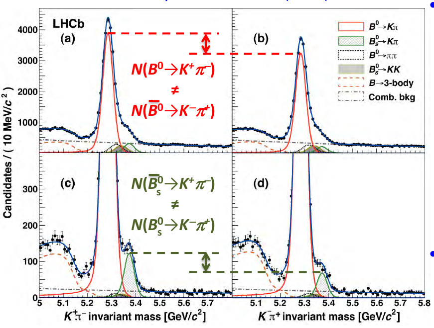
Figure 8: Direct CPV in $B^{0}(B_{s}^{0})\to K\pi$ decays.

0.6.3 25 % direct CP asymmetry in $B_{s}$ decay

While direct CPV in kaons and $D$-mesons is very small it is sometimes huge in B-mesons, see 8 [20].

The diagrams shown in 9 describe $B_{s}\to K^{-}\pi^{+}$ decay.

Figure 9: $B_{s}\to K^{-}\pi^{+}$ decay.

$$A(B_{s}\longrightarrow K^{-}\pi^{+})=T_{s}V^{*}_{ub}V_{ud}+P_{s}e^{i\delta}V^{*}_{cb}V_{cd},$$ (111)

$$A(\bar{B}_{s}\longrightarrow K^{+}\pi^{-})=T_{s}V_{ub}V^{*}_{ud}+P_{s}e^{i\delta}V_{cb}V^{*}_{cd},$$ (112)

where $\delta$ is strong phase; CKM phase is contained in $V_{ub}=-e^{-i\gamma}|V_{ub}|$.

$$A_{CP}(B_{s}\longrightarrow K^{-}\pi^{+})=\frac{|A(\bar{B}_{s})|^{2}-|A(B_{s})|^{2}}{|A(\bar{B}_{s})|^{2}+|A(B_{s})|^{2}}=$$ (113)

$$=\frac{4T_{s}P_{s}V^{*}_{ud}V_{cb}V^{*}_{cd}|V_{ub}|\sin(\delta)\sin(\gamma)}{2T_{s}^{2}|V_{ub}V_{ud}|^{2}+2P_{s}^{2}|V_{cb}V_{cd}|^{2}-4P_{s}T_{s}V^{*}_{ud}V_{cb}V^{*}_{cd}|V_{ub}|\cos(\delta)\cos(\gamma)}.$$

CKM factors in the nominator and denominator are of the order of $\lambda^{6}$ and there is no CKM suppression of $A_{CP}(B_{s})$. Since asymmetry is big, $P_{s}/T_{s}$ is not that small.

Figure 10: $B^{0}\to K^{+}\pi^{-}$ decay.

Though we cannot compute diagrams in 9 and 10, we can relate them in the $U$ spin invariance approximation.

Problem 5

Derive an expression for $A_{CP}(B^{0}\longrightarrow K^{+}\pi^{-})$ and get the following equality:

$$A_{CP}(B^{0})\cdot\Gamma_{B^{0}\rightarrow K\pi}=-A_{CP}(B_{s})\cdot\Gamma_{B_{s}\rightarrow K\pi}\;\;.$$ (114)

Substituting experimentally measured numbers from RPP (PDG) [21] for asymmetries $A_{CP}(B^{0})=-0.082(6),\;\;\;A_{CP}(B_{s})=0.26(4)$ and branching ratios Br($B^{0}\rightarrow K\pi)=20\cdot 10^{-6}$, Br($B_{s}\rightarrow K\pi)=5.7\cdot 10^{-6}$ check this equality.

Smallness of branching ratio of any exclusive decay is the main problem in studying CPV in $B$-mesons.

0.6.4 CPV in neutrino oscillations

In order to have CPV we need not only CP violating phase but CP conserving phase as well ($i\Gamma_{12}$ in case of mixing, $\delta_{2}-\delta_{0}$ in case of direct CPV in kaon decays).

Problem 6

In case of leptons the flavor mixing is described by the PMNS matrix:

$$\left(\begin{array}[]{c}\nu_{e}\\ \nu_{\mu}\\ \nu_{\tau}\end{array}\right)=\left(\begin{array}[]{lll}V_{e1}&V_{e2}&V_{e3}\\ V_{\mu 1}&V_{\mu 2}&V_{\mu 3}\\ V_{\tau 1}&V_{\tau 2}&V_{\tau 3}\end{array}\right)\left(\begin{array}[]{c}\nu_{1}\\ \nu_{2}\\ \nu_{3}\end{array}\right)\;\;.$$ (115)

CPV means in particular that the probability of $\nu_{\mu}\longrightarrow\nu_{e}$ oscillation $P_{e\mu}$ does not coincide with the probability of $\bar{\nu}_{\mu}\longrightarrow\bar{\nu}_{e}$ oscillation $P_{\bar{e}\bar{\mu}}$.

Check that

$$P_{e\mu}-P_{\bar{e}\bar{\mu}}=4Im(V_{\mu 1}^{*}V_{e1}V_{\mu 2}V_{e2}^{*})*[\sin(\frac{\Delta m^{2}_{12}}{2E}x)+\sin(\frac{\Delta m^{2}_{31}}{2E}x)+\sin(\frac{\Delta m^{2}_{23}}{2E}x)].$$ (116)

Just like in kaons CPV is proportional to Jarlskog invariant.

When two neutrinos have equal masses there is no CPV.

Where is the CP conserving phase in the case of CPV in neutrino oscillations?

By the way, the driving force for Bruno Pontecorvo to consider neutrino oscillations was the observed oscillations of neutral kaons [22].

0.6.5 CPV - absolute notion of a particle

$$\delta_{L}=\frac{\Gamma(K_{L}\rightarrow\pi^{-}e^{+}\nu)-\Gamma(K_{L}\rightarrow\pi^{+}e^{-}\bar{\nu})}{\Gamma(K_{L}\rightarrow\pi^{-}e^{+}\nu)+\Gamma(K_{L}\rightarrow\pi^{+}e^{-}\bar{\nu})}=2Re\tilde{\varepsilon}\approx 3.3*10^{-3}.$$ (117)

Pions of low energies mostly produce $K^{0}$ on the Earth, while $\bar{K}^{0}$ on the “antiEarth” ($\pi N\to K^{0}(\Lambda,\Sigma)$; $\pi\bar{N}\to\bar{K}^{0}(\bar{\Lambda},\bar{\Sigma})$). However, in both cases $K_{L}$ decay (a little bit) more often into positrons than into electrons.

“The atoms on the Earth contain antipositrons (electrons) - and what about your planet?”

In this way the measurements of the probabilities of semileptonic $K_{L}$ decays allow to decide if the other planet is made from antimatter.

Problem 7

Violation of leptonic (muon and electron) numbers due to neutrino mixing. Estimate the branching ratio of the $\mu\longrightarrow e\gamma$ decay, which occurs in the Standard Model due to the analog of the penguin diagram from 6 without splitting of the photon.

0.7 Constraints on the unitarity triangle

0.7.1 Parameters of CKM matrix

Four quantities are needed to specify CKM matrix: $s_{12},s_{13},s_{23}$ and $\delta$, or $\lambda,A,\rho,\eta$. The areas shaded in 11 [23] show the domains of $\bar{\rho}$ and $\bar{\eta}$ allowed at 95% C.L. by different measurements ($\bar{\rho}\equiv\rho(1-\lambda^{2}/2),\;\;\bar{\eta}\equiv\eta(1-\lambda^{2}/2)$).

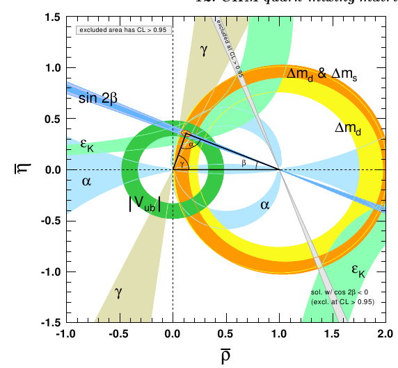
Figure 11: Constraints on the apex of the unitarity triangle.

0.7.2 $V_{cd},V_{cb},V_{ub}$

The precise value of $V_{us}$ follows from the extrapolation of the formfactor of $K\to\pi e\nu$ decay $f_{+}(q^{2})$ to the point $q^{2}=0$, where $q$ is the lepton pair momentum. Due to the Ademollo-Gatto theorem [24] the corrections to the CVC value $f_{+}(0)=1$ are of the second order of flavor SU(3) violation, and these small terms were calculated. (For the case of isotopic SU(2) violation a similar theorem was proved in [25]). As a result of this (and other) analyses PDG gives the following value: $V_{us}\equiv\lambda=0.2243(5)$.

The accuracy of $\lambda$ is high: the other parameters of CKM matrix are known much worse. $V_{cd}$ is measured in the processes with $c$-quark with an order of magnitude worse accuracy: $V_{cd}=0.218(4)$.

The value of $V_{cb}$ is determined from the inclusive and exclusive semileptonic decays of $B$-mesons to charm. At the level of quarks $b\to cl\nu$ transition is responsible for these decays: $V_{cb}=(42.2\pm 0.8)\cdot 10^{-3}$.

The value of $|V_{ub}|$ is extracted from the semileptonic $B$-mesons decays without the charmed particles in the final state which originated from $b\to ul\nu$ transition: $V_{ub}=(3.94\pm 0.36)\cdot 10^{-3}$.

The apex of the unitarity triangle should belong to a circle on $(\bar{\rho},\bar{\eta})$ plane with the center at the point $(0,0)$. The area between such two circles (deep green color) corresponds to the domain allowed at $2\sigma$.

0.7.3 $\varepsilon_{K},\Delta m_{B^{0}},\Delta m_{B^{0}_{s}}$

CPV in kaon mixing determines the hyperbola shown by light green color in 11, see Eq.(87).

Figure 12: $B^{0}$ – $\bar{B}^{0}$ mixing.

In Standard Model $B_{d}-\bar{B}_{d}$ transition occurs through the box diagram shown in 12. Unlike the case of $K^{0}-\bar{K}^{0}$ transition the power of $\lambda$ is the same for $u$, $c$ and $t$ quarks inside a loop, so the diagram with $t$-quarks dominates.

Calculating it in complete analogy with $K$-meson case we get:

$$M_{12}=-\frac{G_{F}^{2}B_{B_{d}}f_{B_{d}}^{2}}{12\pi^{2}}m_{B}m_{t}^{2}\eta_{B}V_{tb}^{2}V_{td}^{*^{2}}I(\xi)\;\;,$$ (118)

where $I(\xi)$ is the same function as that for $K$-mesons, $\eta_{B}=0.55\pm 0.01$ (NLO).

$\Gamma_{12}$ is determined by the absorptive part of the same diagram (so, 4 diagrams altogether: $uu$, $uc$, $cu$, $cc$ quarks in the inner lines). The result of calculation is:

$$\Gamma_{12}=\frac{G_{F}^{2}B_{B_{d}}f_{B_{d}}^{2}m_{B}^{3}}{8\pi}[V_{cb}V_{cd}^{*}(1+O(\frac{m_{c}^{2}}{m_{b}^{2}}))+V_{ub}V_{ud}^{*}]^{2}\;\;,$$ (119)

where the term $O(m_{c}^{2}/m_{b}^{2})$ accounts for nonzero $c$-quark mass.

Using the unitarity of CKM matrix we get:

$$\Gamma_{12}=\frac{G_{F}^{2}B_{B_{d}}f_{B_{d}}^{2}m_{B}^{3}}{8\pi}[-V_{tb}V_{td}^{*}+O(\frac{m_{c}^{2}}{m_{b}^{2}})V_{cb}V_{cd}^{*}]^{2}\;\;,$$ (120)

and the main term in $\Gamma_{12}$ has the same phase as the main term in $M_{12}$. That is why CPV in mixing of $B$-mesons is suppressed by an extra factor $(m_{c}/m_{b})^{2}$ and is small. For the difference of masses of the two eigenstates from

$$M_{+}-M_{-}-\frac{i}{2}(\Gamma_{+}-\Gamma_{-})=2\sqrt{(M_{12}-\frac{i}{2}\Gamma_{12})(M_{12}^{*}-\frac{i}{2}\Gamma_{12}^{*})}$$ (121)

we obtain:

$$\Delta m_{B^{0}}=-\frac{G_{F}^{2}B_{B_{d}}f_{B}^{2}}{6\pi^{2}}m_{B}m_{t}^{2}\eta_{B}\mid V_{tb}^{2}V_{td}^{*^{2}}\mid I(\xi),$$ (122)

and $\Delta m_{B^{0}}$ is negative as well as in the kaon system: a heavier state has a smaller width.

0.7.4 $\Delta m_{B^{0}}$ and semileptonic $B^{0}(\bar{B}^{0})$ decays

The $B$-meson semileptonic decays are induced by a semileptonic $b$-quark decay, $b\to cl^{-}\nu\;\;(ul^{-}\nu)$. In this way in the decays of $\bar{B}^{0}$ mesons $l^{-}$ are produced, while in the decays of $B^{0}$ mesons $l^{+}$ are produced. However, $B^{0}$ and $\bar{B}^{0}$ are not the mass eigenstates and being produced at $t=0$ they start to oscillate according to the following formulas:

$$B^{0}(t)=\frac{e^{-i\lambda_{+}t}+e^{-i\lambda_{-}t}}{2}B^{0}+\frac{q}{p}\frac{e^{-i\lambda_{+}t}-e^{-i\lambda_{-}t}}{2}\bar{B}^{0}\;\;,$$ (123)

$$\bar{B}^{0}(t)=\frac{e^{-i\lambda_{+}t}+e^{-i\lambda_{-}t}}{2}\bar{B}^{0}+\frac{p}{q}\frac{e^{-i\lambda_{+}t}-e^{-i\lambda_{-}t}}{2}B^{0}\;\;.$$ (124)

That is why in their semileptonic decays the “wrong sign leptons” are sometimes produced, $l^{-}$ in the decays of the particles born as $B^{0}$ and $l^{+}$ in the decays of the particles born as $\bar{B}^{0}$. The number of these “wrong sign” events depends on the ratio of the oscillation frequency $\Delta m$ and $B$-meson lifetime $\Gamma$ (unlike the case of $K$-mesons for $B$-mesons $\Delta\Gamma\ll\Gamma$). For $\Delta m\gg\Gamma$ a large number of oscillations occurs, and the number of “the wrong sign leptons” equals that of a normal sign. If $\Delta m\ll\Gamma$, then $B$-mesons decay before they start to oscillate.

The pioneering detection of “the wrong sign events” by ARGUS collaboration in 1987 demonstrated that $\Delta m$ is of the order of $\Gamma$, which in the framework of Standard Model could be understood only if the top quark is unusually heavy, $m_{t}\geq 100$ GeV [26]. Fast $B^{0}-\bar{B}^{0}$ oscillations made possible the construction of asymmetric $B$-factories (suggested in [27]) where CPV in $B^{0}$ decays was observed. (Let us mention that UA1 collaboration saw the events which were interpreted as a possible manifestation of $B_{s}^{0}-\bar{B}_{s}^{0}$ oscillations [28].)

Integrating the probabilities of $B^{0}$ decays in $l^{+}$ and $l^{-}$ over $t$, we obtain for “the wrong sign lepton” probability:

$$W_{B^{0}\to\bar{B}^{0}}\equiv\frac{N_{B^{0}\to l^{-}X}}{N_{B^{0}\to l^{-}X}+N_{B^{0}\to l^{+}X}}=\frac{\mid\frac{q}{p}\mid^{2}(\frac{\Delta m}{\Gamma})^{2}}{2+(\frac{\Delta m}{\Gamma})^{2}+\mid\frac{q}{p}\mid^{2}(\frac{\Delta m}{\Gamma})^{2}}\;\;,$$ (125)

where we neglect $\Delta\Gamma$, the difference of $B_{+}$- and $B_{-}$-mesons lifetimes. Precisely according to our discussion for $\Delta m/\Gamma\gg 1$ we have $W=1/2$, while for $\Delta m/\Gamma\ll\ 1$ we have $W=1/2(\Delta m/\Gamma)^{2}$ (with high accuracy $\mid p/q\mid=1$).

For $\bar{B}^{0}$ decays we get the same formula with the interchange of $q$ and $p$.

In ARGUS experiment $B$-mesons were produced in $\Upsilon(4S)$ decays: $\Upsilon(4S)\to B\bar{B}$. $\Upsilon$ resonances have $J^{PC}=1^{--}$, that is why (pseudo)scalar $B$-mesons are produced in $P$-wave. It means that $B\bar{B}$ wave function is antisymmetric at the interchange of $B$ and $\bar{B}$. This fact forbids the configurations in which due to $B-\bar{B}$ oscillations both mesons become $B$, or both become $\bar{B}$. However, after one of the $B$-meson decays the flavor of the remaining one is tagged, and it oscillates according to (123), (124).

If the first decay is semileptonic with $l^{+}$ emission indicating that a decaying particle was $B^{0}$, then the second particle was initially $\bar{B}^{0}$. Thus taking $\mid p/q\mid=1$ we get for the relative number of the same sign dileptons born in semileptonic decays of $B$-mesons, produced in $\Upsilon(4S)\to B\bar{B}$ decays:

$$\frac{N_{l^{+}l^{+}}+N_{l^{-}l^{-}}}{N_{l^{+}l^{-}}}=\frac{W}{1-W}=\frac{x^{2}}{2+x^{2}}\;,\;\;x\equiv\frac{\Delta m}{\Gamma}\;\;.$$ (126)

Let us note that if $B^{0}$ and $\bar{B}^{0}$ are produced incoherently (say, in hadron collisions) a different formula should be used:

$$\frac{N_{l^{+}l^{+}}+N_{l^{-}l^{-}}}{N_{l^{+}l^{-}}}=\frac{2W-2W^{2}}{1-2W+2W^{2}}=\frac{x^{2}(2+x^{2})}{2+2x^{2}+x^{4}}\;\;.$$ (127)

In the absence of oscillations ($x=0$) both equations give zero; for high frequency oscillations ($x\gg 1$) both of them give one.

From the time integrated data of ARGUS and CLEO $W_{d}=0.182\pm 0.015$ follows. From the time-dependent analysis of $B$-decays at the high energy colliders (LEP II, Tevatron, SLC, LHC) and the time-dependent analysis at the asymmetric $B$-factories Belle and BaBar the following result was obtained :

$$x_{d}=0.770(4)\;\;.$$ (128)

By using the life time of $B_{d}$-mesons: $\Gamma_{B_{d}}=[1.52(1)\cdot 10^{-12}\;{\rm sec}]^{-1}\equiv[1.52(1){\rm ps}]^{-1}$ we get for the mass difference of $B_{d}$ mesons:

$$\Delta m_{d}=0.506(2){\rm ps}^{-1}\;\;{\rm or,\;equivalently},W_{d}=0.1874\pm 0.0018.$$ (129)

This $\Delta m_{d}$ value can be used in Eq.(122) to extract the value of $|V_{td}|$. The main uncertainty is in a hadronic matrix element $f_{B_{d}}\sqrt{B_{B_{d}}}=216\pm 15$ MeV obtained from the lattice QCD calculations.

0.7.5 $\Delta m_{B^{0}_{s}}$

Theoretical uncertainty diminishes in the ratio

$$\frac{\Delta m_{s}}{\Delta m_{d}}=\frac{m_{B_{s}}}{m_{B_{d}}}\xi^{2}\frac{|V_{ts}|^{2}}{|V_{td}|^{2}},$$ (130)

where $\xi=(f_{B_{s}}\sqrt{B_{B_{s}}})/(f_{B_{d}}\sqrt{B_{B_{d}}})=1.24\pm 0.05$.

Since the lifetimes of $B_{d}$ - and $B_{s}$ -mesons are almost equal, we get:

$$x_{s}\approx x_{d}\frac{|V_{ts}|^{2}}{|V_{td}|^{2}}$$ (131)

which means $x_{s}\gg 1$ and very fast oscillations. That is why $W_{B_{s}}$ equals $1/2$ with very high accuracy and one cannot extract $x_{B_{s}}$ from the time integrated measurements.

$B^{0}_{s}-\bar{B}^{0}_{s}$ oscillations were first observed at Tevatron. The average of all published measurements

$$\Delta m_{B^{0}_{s}}=17.757\pm 0.020{\rm(stat)}\pm 0.007{\rm(syst)\;\;(ps}^{-1})$$ (132)

is dominated by LHCb.

Thus we get

$$|V_{td}/V_{ts}|=0.210\pm 0.001({\rm exp})\pm 0.008({\rm theor}),$$ (133)

which corresponds to yellow (only $\Delta m_{d}$) and brown ($\Delta m_{d}$ and $\Delta m_{s}$) circles in 11.

What remains is the values of the angles of the unitarity triangle, which are determined by CP-violation measurements in B-meson decays. Soon we will go there.

0.7.6 $\Delta\Gamma/\Gamma$

For the difference of the width of $B_{dL}$ and $B_{dH}$ we obtain

$$\Delta\Gamma_{B_{d}}=2\Gamma_{12}\approx\frac{G_{F}^{2}B_{B_{d}}f_{B}^{2}m_{B}^{3}}{4\pi}\mid V_{td}\mid^{2}\;\;,$$ (134)

which is very small:

$$\frac{\Delta\Gamma_{B_{d}}}{\Gamma_{B_{d}}}<1{\rm\%}\ \;\;,$$ (135)

as opposite to $K$-meson case, where $K_{S}$ and $K_{L}$ lifetimes differ strongly.

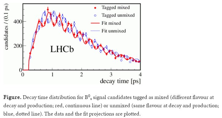
Figure 13: $B_{s}$ – $\bar{B}_{s}$ oscillations [29].

In the $B_{s}$-meson system a larger time difference was expected; substituting $V_{ts}$ instead of $V_{td}$ we obtain:

$$\frac{\Delta\Gamma_{B_{s}}}{\Gamma_{B_{s}}}\sim 10{\rm\%}\;\;.$$ (136)

Here are experimental results:

$$\Gamma_{B^{0}_{sL}}=(1.414(10){\rm ps})^{-1}$$ (137)

$$\Gamma_{B^{0}_{sH}}=(1.624(14){\rm ps})^{-1},$$ (138)

where L is light, H - heavy.

0.8 CPV in $B^{0}-\bar{B}^{0}$ mixing

For a long time CPV in $K$-mesons was observed only in $K^{0}-\bar{K}^{0}$ mixing. That is why it seems reasonable to start studying CPV in $B$-mesons from their mixing:

$$\left|\frac{q}{p}\right|=\left|\sqrt{1+\frac{i}{2}\left(\frac{\Gamma_{12}}{M_{12}}-\frac{\Gamma_{12}^{*}}{M_{12}^{*}}\right)}\right|=\left|1+\frac{i}{4}\left(\frac{\Gamma_{12}}{M_{12}}-\frac{\Gamma_{12}^{*}}{M_{12}^{*}}\right)\right|=$$

$$=1-\frac{1}{2}{\rm Im}\left(\frac{\Gamma_{12}}{M_{12}}\right)\approx 1-\frac{m_{c}^{2}}{m_{t}^{2}}{\rm Im}\frac{V_{cb}V_{cd}^{*}}{V_{tb}V_{td}^{*}}\approx 1-O(10^{-4})\;\;.$$ (139)

We see that CPV in $B_{d}-\bar{B}_{d}$ mixing is very small because $t$-quark is very heavy and is even smaller in $B_{s}-\bar{B}_{s}$ mixing.

The experimental observation of $B_{d}-\bar{B}_{d}$ mixing comes from the detection of the same sign leptons produced in the semileptonic decays of $B_{d}-\bar{B}_{d}$ pair from $\Upsilon(4S)$ decay. Due to CPV in the mixing the number of $l^{-}l^{-}$ events will differ from that of $l^{+}l^{+}$ and this difference is proportional to $|\frac{q}{p}|-1\sim 10^{-4}$:

$$A_{SL}^{B}=\frac{N(\bar{B}^{0}\to l^{+}X)-N(B^{0}\to l^{-}X)}{N(\bar{B}^{0}\to l^{+}X)+N(B^{0}\to l^{-}X)}=O(10^{-4}).$$ (140)

The experimental number is:

$$A_{SL}^{B_{d}}=0.0021\pm 0.0017\;\;,$$ (141)

or

$$|q/p|_{B_{d}}=1.0010\pm 0.0008\;\;.$$ (142)

This result shows no evidence of CPV and does not constrain the SM.

0.9 CPV in interference of mixing and decays, $B^{0}(\bar{B}^{0})\to J/\Psi K$, angle $\beta$.

0.9.1 General formulae.

As soon as it became clear that CPV in $B-\bar{B}$ mixing is small theoreticians started to look for another way to find CPV in $B$ decays. The evident alternative is the direct CPV. It is very small in $K$-mesons because: a) the third generation almost decouples in $K$ decays; b) due to $\Delta I=1/2$ rule. Since in $B$-meson decays all three quark generations are involved and there are many different final states, large direct CPV does occur [30] - [33]. An evident drawback of this strategy: a branching ratio of $B$-meson decays into any particular exclusive hadronic mode is very small (just because there are many modes available), so a large number of $B$-meson decays are needed. The specially constructed asymmetric $e^{+}e^{-}$-factories Belle (1999-2010) and BaBar (1999-2008) working at the invariant mass of $\Upsilon(4S)$ discovered CPV in $B^{0}(\bar{B}^{0})$ decays in 2001 [16].

The time evolution of the states produced at $t=0$ as $B^{0}$ or $\bar{B}^{0}$ is described by (123), (124). It is convenient to present these formulae in a little bit different form:

$$\mid B^{0}(t)>=e^{-i\frac{M_{+}+M_{-}}{2}t-\frac{\Gamma t}{2}}\left[\cos(\frac{\Delta mt}{2})\mid B^{0}>+i\frac{q}{p}\sin(\frac{\Delta mt}{2})\mid\bar{B}^{0}>\right]\;\;,$$ (143)

$$\mid\bar{B}^{0}(t)>=e^{-i\frac{M_{+}+M_{-}}{2}t-\frac{\Gamma t}{2}}\left[+i\frac{p}{q}\sin(\frac{\Delta mt}{2})\mid B^{0}>+\cos(\frac{\Delta mt}{2})\mid\bar{B}^{0}>\right]\;,$$ (144)

where $\Delta m\equiv M_{-}-M_{+}>0$, and we take $\Gamma_{+}=\Gamma_{-}=\Gamma$ neglecting their small difference (which should be accounted for in case of $B_{s}$).

Let us consider a decay in some final state $f$. Introducing the decay amplitudes according to the following definitions:

$$A_{f}=A(B^{0}\to f)\;,\;\;\bar{A}_{f}=A(\bar{B}_{0}\to f)\;\;,$$ (145)

$$A_{\bar{f}}=A(B^{0}\to\bar{f})\;,\;\;\bar{A}_{\bar{f}}=A(\bar{B}_{0}\to\bar{f})\;\;,$$ (146)

for the decay probabilities as functions of time we obtain:

$$P_{B^{0}\to f}(t)=e^{-\Gamma t}\mid A_{f}\mid^{2}\left[\cos^{2}(\frac{\Delta mt}{2})+\left|\frac{q\bar{A}_{f}}{pA_{f}}\right|^{2}\sin^{2}(\frac{\Delta mt}{2})-{\rm Im}\left(\frac{q\bar{A}_{f}}{pA_{f}}\right)\sin(\Delta mt)\right]\;\;,$$ (147)

$$P_{\bar{B}^{0}\to\bar{f}}(t)=e^{-\Gamma t}\mid\bar{A}_{\bar{f}}\mid^{2}\left[\cos^{2}(\frac{\Delta mt}{2})+\left|\frac{pA_{\bar{f}}}{q\bar{A}_{\bar{f}}}\right|^{2}\sin^{2}(\frac{\Delta mt}{2})-{\rm Im}\left(\frac{pA_{\bar{f}}}{q\bar{A}_{\bar{f}}}\right)\sin(\Delta mt)\right]\;\;.$$ (148)

The difference of these two probabilities signals different types of CPV: the difference in the first term in brackets appears due to direct CPV; the difference in the second term - due to CPV in mixing or due to direct CPV, and in the last term – due to CPV in the interference of $B^{0}-\bar{B}^{0}$ mixing and decays.

Let $f$ be a CP eigenstate: $\bar{f}=\eta_{f}f$, where $\eta_{f}=+(-)$ for CP even (odd) $f$. (Two examples of such decays: $B^{0}\to J/\Psi K_{S(L)}$ and $B^{0}\to\pi^{+}\pi^{-}$ are described by the quark diagrams shown in 14. The analogous diagrams describe $\bar{B}^{0}$ decays in the same final states.) The following equalities can be easily obtained:

$$A_{\bar{f}}=\eta_{f}A_{f}\;,\;\;\bar{A}_{\bar{f}}=\eta_{f}\bar{A}_{f}\;\;.$$ (149)

Figure 14: Quark diagrams responsible for $B^{0}\to J/\Psi K$ and $B^{0}\to\pi\pi$-decays.

In the absence of CPV the expressions in brackets are equal and the obtained formulas describe the exponential particle decay without oscillations. Taking CPV into account and neglecting a small deviation of $\mid p/q\mid$ from one, for CPV asymmetry of the decays into CP eigenstate we obtain:

$$a_{CP}(t)\equiv\frac{P_{\bar{B}^{0}\to f}-P_{B^{0}\to f}}{P_{\bar{B}^{0}\to f}+P_{B_{0}\to f}}=\frac{\mid\lambda\mid^{2}-1}{\mid\lambda\mid^{2}+1}\cos(\Delta mt)+\frac{2Im\lambda}{\mid\lambda\mid^{2}+1}\sin(\Delta mt)\equiv$$

$$\equiv-C_{f}\cos(\Delta mt)+S_{f}\sin(\Delta mt)\;\;,$$ (150)

where $\lambda\equiv\frac{q\bar{A}_{f}}{pA_{f}}$. (Do not confuse with the parameter of CKM matrix).

The nonzero value of $C_{f}$ corresponds to direct CPV; it occurs when more than one amplitude contribute to the decay. For extraction of CPV parameters (the angles of the unitarity triangle) in this case the knowledge of strong rescattering phases is necessary. The nonvanishing $S_{f}$ describes CPV in the interference of mixing and decay. It is nonzero even when there is only one decay amplitude, and $|\lambda|=1$. Such decays are of special interest since the extraction of CPV parameters becomes independent of poorly known strong phases of the final particles rescattering.

The decays of $\Upsilon(4S)$ resonance produced in $e^{+}e^{-}$ annihilation are a powerful source of $B^{0}\bar{B}^{0}$ pairs. A semileptonic decay of one of the $B$’s tags “beauty” of the partner at the moment of decay (since $(B^{0}B^{0}),(\bar{B}^{0}\bar{B}^{0})$ states are forbidden) thus making it possible to study CPV. However, the time-integrated asymmetry is zero for decays were $C_{f}$ is zero. This happens since we do not know which of the two $B$-mesons decays earlier, and asymmetry is proportional to: $I=\int\limits^{\infty}_{-\infty}e^{-\Gamma|t|}\sin(\Delta mt)dt=0\;\;.$ The asymmetric $B$-factories provide possibility to measure the time-dependence: $\Upsilon(4S)$ moves in a laboratory system, and since energy release in $\Upsilon(4S)\to B\bar{B}$ decay is very small both $B$ and $\bar{B}$ move with the same velocity as the original $\Upsilon(4S)$. This makes the resolution of $B$ decay vertices possible unlike the case of $\Upsilon(4S)$ decay at rest, when non-relativistic $B$ and $\bar{B}$ decay at almost the same point. The implementation of the time-dependent analysis for the search of CPV in $B$-mesons was suggested in [34] - [36].

0.9.2 $B_{d}^{0}(\bar{B}_{d}^{0})\to J/\Psi K_{S(L)}$, $\sin 2\beta$ – straight lines

The tree diagram contributing to this decay is shown in 14 a). The product of the corresponding CKM matrix elements is: $V_{cb}^{*}V_{cs}\simeq A\lambda^{2}$. Also the penguin diagram $b\to sg$ with the subsequent $g\to c\bar{c}$ decay contributes to the decay amplitude. Its contribution is proportional to:

$$P\sim V_{us}V_{ub}^{*}f(m_{u})+V_{cs}V_{cb}^{*}f(m_{c})+V_{ts}V_{tb}^{*}f(m_{t})=$$

$$=V_{us}V_{ub}^{*}(f(m_{u})-f(m_{t}))+V_{cs}V_{cb}^{*}(f(m_{c})-f(m_{t}))\;\;,$$ (151)

where function $f$ describes the contribution of quark loop and we have subtracted zero from the expression on the first line. The last term on the second line has the same weak phase as the tree amplitude, while the first term has a CKM factor $V_{us}V_{ub}^{*}\sim\lambda^{4}(\rho-i\eta)A$. Since (one-loop) penguin amplitude should be in any case smaller than the tree one, we get that with 1% accuracy there is only one weak amplitude governing $B_{d}^{0}(\bar{B}_{d}^{0})\to J/\Psi K_{S(L)}$ decays. This is the reason why this mode is called a “gold-plated mode” – the accuracy of the theoretical prediction of the CP-asymmetry is very high, and Br $(B_{d}\to J/\Psi K^{0})\approx 10^{-3}$ is large enough to detect CPV.

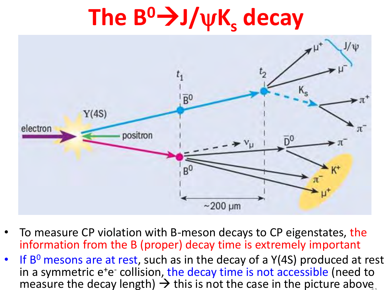
Figure 15: Tagging $\bar{B}^{0}$-meson by $B^{0}$-decay.

Substituting $|\lambda|=1$ in the expression for $a_{CP}(t)$ we obtain:

$$a_{CP}(t)={\rm Im}\lambda\sin(\Delta m\Delta t)\;\;,$$ (152)

where $\Delta t$ is the time difference between the semileptonic decay of one of $B$-mesons produced in $\Upsilon(4S)$ decay and that of the second one to $J/\Psi K_{S(L)}$. Using the following equation

$$\bar{A}_{f}=\eta_{f}\bar{A}_{\bar{f}}\;\;,$$ (153)

where $\eta_{f}$ is CP parity of the final state, we obtain:

$$\lambda=\left(\frac{q}{p}\right)_{B_{d}}\frac{A_{\bar{B}^{0}\to J/\Psi K_{S(L)}}}{A_{B^{0}\to J/\Psi K_{S(L)}}}=\left(\frac{q}{p}\right)_{B_{d}}\eta_{f}\frac{A_{\bar{B}^{0}\to\overline{J/\Psi K_{S(L)}}}}{A_{B^{0}\to J/\Psi K_{S(L)}}}\;\;.$$ (154)

The amplitude in the nominator contains $\bar{K}^{0}$ production. To project it on $\bar{K}_{S(L)}$ we should use:

$$\overline{K^{0}}=\frac{K_{S}-K_{L}}{(q)_{K}}=\frac{\bar{K}_{S}+\bar{K}_{L}}{(q)_{K}}\;\;,$$ (155)

getting $(q)_{K}$ in the denominator. The amplitude in the denominator contains $K^{0}$ production, and using:

$$K^{0}=\frac{K_{S}+K_{L}}{(p)_{K}}$$ (156)

we obtain factor $(p)_{K}$ in the nominator. Collecting all the factors together and substituting CKM matrix elements for $\bar{A}_{\bar{f}}/A_{f}$ ratio we get:

$$\lambda=\eta_{S(L)}\left(\frac{q}{p}\right)_{B_{d}}\frac{V_{cb}V_{cs}^{*}}{V_{cb}^{*}V_{cs}}\left(\frac{p}{q}\right)_{K}\;\;.$$ (157)

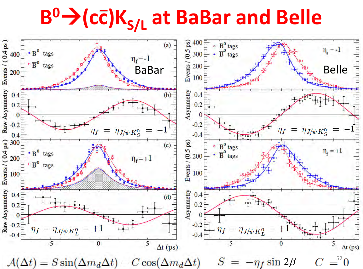
Figure 16: Measurements of CPV asymmetries.

Substituting the expressions for $(q/p)_{B_{d}}$ and $(p/q)_{K}$ we obtain:

$$\lambda(J/\Psi K_{S(L)})=\eta_{S(L)}\frac{V_{td}V_{tb}^{*}}{V_{td}^{*}V_{tb}}\frac{V_{cb}V_{cs}^{*}}{V_{cb}^{*}V_{cs}}\frac{V_{cd}^{*}V_{cs}}{V_{cd}V_{cs}^{*}}\;\;,$$ (158)

which is invariant under the phase rotation of any quark field. From the unitarity triangle figure we have

$$\arg(V_{tb}^{*}V_{td})=\pi-\beta\;\;,$$ (159)

and we finally obtain:

$$a_{CP}(t)\left|{}_{{}_{{}_{{}_{\large J/\Psi K_{S(L)}}}}}=-\eta_{S(L)}\sin(2\beta)\sin(\Delta m\Delta t)\right.\;\;,$$ (160)

which is a simple prediction of the Standard Model. Since in $B$ decays $J/\Psi$ and $K_{S(L)}$ are produced in $P$-wave, $\eta_{S(L)}=-1(+1)$ (CP of $J/\Psi$ is $+1$, that of $K_{S}$ is $+1$ as well, and $(-1)^{l}=-1$ comes from $P$-wave; CP of $K_{L}$ is $-1$).

In this way the measurement of this asymmetry at $B$-factories provides the value of angle $\beta$ of the unitarity triangle. The Belle, BaBar and LHCb average is:

$$\sin 2\beta=0.691\pm 0.017\;\;,$$ (161)

which corresponds to

$$\beta=(21.9\pm 0.7)^{0}.$$ (162)

As a final state not only $J/\Psi K_{S(L)}$ were selected, but neutral kaons with the other charmonium states as well.

Let us note that the decay amplitudes and $K^{0}-\bar{K}^{0}$ mixing do not contain a complex phase, that is why the only source of it in $B^{0}\to{\rm charmonium}\;K_{S(L)}$ decays is $B^{0}-\bar{B}^{0}$ mixing:

$$\left(\frac{q}{p}\right)_{B_{d}}=\sqrt{\frac{M_{12}^{*}}{M_{12}}}=\frac{V_{tb}^{*}V_{td}}{V_{tb}V_{td}^{*}}\;\;,$$ (163)

thus the phase comes from $V_{td}$, that is why the final expression contains angle $2\beta$ – the phase of $V_{td}/V_{td}^{*}$.

15 and 16 (see [37]) illustrate the above discussion.

0.10 What is the probability of $\Upsilon(4S)\rightarrow B_{d}^{0}\bar{B}_{d}^{0}\to J/\Psi K_{S}\;J/\Psi K_{S}$ decay?

The following parameters are used to describe the time evolution of $B$-mesons: $m\equiv(m_{H}+m_{L})/2\;,\;\;\Delta m\equiv m_{H}-m_{L}\;,\;\;\Gamma_{H}=\Gamma_{L}=\Gamma\;.$

Since $J^{PC}(\Upsilon)=1^{--}$, $B$-mesons are produced in P-wave, so their wave function is $C$-odd: $\Psi(t_{1},t_{2})=B^{0}(t_{1})\bar{B}^{0}(t_{2})-B^{0}(t_{2})\bar{B}^{0}(t_{1}).$

For the decay amplitude we get:

$$\left<J/\Psi K_{S}\;J/\Psi K_{S}|\Psi(t_{1},t_{2})\right>=e^{-imt_{1}-\frac{\Gamma t_{1}}{2}}\left[A\cos\frac{\Delta mt_{1}}{2}+i\frac{q}{p}\sin\left(\frac{\Delta mt_{1}}{2}\right)\bar{A}\right]\times$$

$$\times e^{-imt_{2}-\frac{\Gamma t_{2}}{2}}\left[\cos\left(\frac{\Delta mt_{2}}{2}\right)\bar{A}+i\frac{p}{q}\sin\left(\frac{\Delta mt_{2}}{2}\right)A\right]-(t_{1}\leftrightarrow t_{2})=\leavevmode\nobreak\ \leavevmode\nobreak\ \leavevmode\nobreak\$$ (164)

$$=e^{-im(t_{1}+t_{2})-\Gamma\frac{t_{1}+t_{2}}{2}}\left[(i\frac{p}{q}A^{2}-i\frac{q}{p}\bar{A}^{2})\cos\left(\frac{\Delta mt_{1}}{2}\right)\sin\left(\frac{\Delta mt_{2}}{2}\right)\right.+$$

$$+\left.(i\frac{q}{p}\bar{A}^{2}-i\frac{p}{q}A^{2})\sin\left(\frac{\Delta mt_{1}}{2}\right)\cos\left(\frac{\Delta mt_{2}}{2}\right)\right]=-e^{-2imt-\Gamma t}(i\frac{p}{q}A^{2})[1-\lambda^{2}]\sin\left(\frac{\Delta m\Delta t}{2}\right)\;\;,$$

where $t\equiv\frac{t_{1}+t_{2}}{2}\;,\Delta t\equiv t_{1}-t_{2},\;\;\frac{q}{p}=e^{-2i\beta}.$

Decay probability equals

$$P(J/\Psi K_{S},J/\Psi K_{S})=e^{-2\Gamma t}|A|^{4}[1-e^{4i\beta}][1-e^{-4i\beta}]\sin^{2}\left(\frac{\Delta m\Delta t}{2}\right)\sim e^{-2\Gamma t}\sin^{2}(2\beta)\sin^{2}\frac{(\Delta m\Delta t)}{2}\;.$$ (165)

Changing integration variables in the expression for decay probability according to

$$\int\limits_{0}^{\infty}dt_{1}\int\limits_{0}^{\infty}dt_{2}=\int\limits_{-\infty}^{\infty}d(\Delta t)\int\limits_{|\Delta t|/2}^{\infty}dt$$ (166)

and performing integration over $t$ we get:

$$N(\Delta t)\sim\sin^{2}2\beta[1-\cos(\Delta m\Delta t)]e^{-\Gamma|\Delta t|}\;\;,$$ (167)

which is zero when $\Delta t=0$ due to Bose statistics, when $\Delta m=0$ – no oscillations, and for $\beta=0$ – no CPV (CP $\Upsilon=+$, CP $(J/\Psi K_{S}\;J/\Psi K_{S})=-$).

For the total number of $\Upsilon(4S)\to J/\Psi K_{S}\;J/\Psi K_{S}$ decays integrating over $\Delta t$ we obtain:

$$N(J/\Psi K_{S}\;J/\Psi K_{S})\sim\sin^{2}2\beta\left(\frac{\Delta m^{2}}{\Delta m^{2}+\Gamma^{2}}\right)$$ (168)

After one of $B$ decays to $J/\Psi K_{S}$ the second one starts to oscillate and may decay to $J/\Psi K_{S}$ as well. The initial state is $CP$ even, the final state is $CP$ odd, so no decays without CPV would occur.

Taking different initial and final states one may solve many problems the same way as we have just shown.

$C$-even initial state:

$$\Psi(t_{1},t_{2})=B^{0}(t_{1})\bar{B}^{0}(t_{2})+B^{0}(t_{2})\bar{B}^{0}(t_{1})\;\;.$$ (169)

The "classical“ initial state (produced in hadron collisions):

$$\Psi(t_{1},t_{2})=B^{0}(t_{1})\bar{B}^{0}(t_{2})\;\;.$$ (170)

0.11 CPV in $b\to sg\to ss\bar{s}$ transition: penguin domination

The decays $B_{d}\to\phi K^{0},K^{+}K^{-}K^{0},\eta^{\prime}K^{0}$ proceed through the diagrams shown in 17.

Figure 17: Penguin diagram describing $b\to ss\bar{s}$-transition.

The diagram with an intermediate $u$-quark is proportional to $\lambda^{4}$, while those with intermediate $c$- and $t$-quarks are proportional to $\lambda^{2}$. In this way the main part of the decay amplitude is free of CKM phase, just like in case of $B_{d}\to J/\Psi K$ decays. A nonzero phase which leads to time-dependent CP asymmetry comes from $B_{d}-\bar{B}_{d}$ transition:

$$a_{CP}(t)=-\eta_{f}\sin(2\beta)\sin(\Delta m\Delta t)\;\;,$$ (171)

analogously to $B_{d}\to J/\Psi K$ decays.

The main interest in these decays is to look for phases of NP which may be hidden in loops. According to 18 [38] SM nicely describes the experimental data within their present day accuracy.

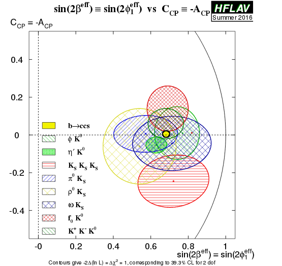
Figure 18: CP-asymmetries from $B_{d}$-decays with production of three strange quarks.

0.12 $B_{s}(\bar{B}_{s})\to J/\Psi\phi$, $\phi_{s}$

This decay is an analog of $B^{0}(\bar{B}^{0})\to J/\Psi K$ decay: the tree amplitude dominates and CP asymmetry could appear from $B_{s}\leftrightarrow\bar{B}_{s}$ transition. $V_{ts}$ unlike $V_{td}$ is almost real, so asymmetry should be very small in SM – a good place to look for New Physics. The angular analysis of $J/\Psi\rightarrow\mu^{+}\mu^{-}$ and $\phi\rightarrow KK$ decays is necessary to select the final states with definite CP parity.

Taking the difference of the width of two eigenstates into account ($\Delta\Gamma=\Gamma_{L}-\Gamma_{H}$) we get:

$$P_{B_{s}\to f}(t)=\frac{1}{2}e^{-\Gamma t}|A_{f}|^{2}(1+|\lambda_{f}|^{2})[\cosh(\Delta\Gamma t/2)-D_{f}\sinh(\Delta\Gamma t/2)+C_{f}\cos(\Delta mt)-S_{f}\sin(\Delta mt)]\;\;,$$ (172)

$$P_{\bar{B}_{s}\to f}(t)=\frac{1}{2}e^{-\Gamma t}|\frac{p}{q}A_{f}|^{2}(1+|\lambda_{f}|^{2})[\cosh(\Delta\Gamma t/2)-D_{f}\sinh(\Delta\Gamma t/2)-C_{f}\cos(\Delta mt)+S_{f}\sin(\Delta mt)]\;\;,$$ (173)

$$D_{f}=\frac{2Re\lambda_{f}}{1+|\lambda_{f}|^{2}},\;\;\;C_{f}=\frac{1-|\lambda_{f}|^{2}}{1+|\lambda_{f}|^{2}},\;\;\;S_{f}=\frac{2Im\lambda_{f}}{1+|\lambda_{f}|^{2}}\;\;.$$ (174)

$$A_{CP}(t)(|p/q|=1)=\frac{-C_{f}\cos(\Delta mt)+S_{f}\sin(\Delta mt)}{\cosh(\Delta\Gamma t/2)-D_{f}\sinh(\Delta\Gamma t/2)}\;\;.$$ (175)

Standard Model prediction is $\phi_{s}^{SM}=-$arg$\frac{V_{ts}V_{tb}^{*}}{V_{ts}^{*}V_{tb}}=-2\lambda^{2}\eta$ =-0.036 rad, while $\phi_{s}^{exp}=-0.040\pm 0.025$ rad. No New Physics in this decay as well.

0.13 Angles $\alpha$ and $\gamma$

0.13.1 $\alpha:B\longrightarrow\pi\pi,\rho\rho,\pi\rho$

Since $\alpha$ is the angle between $V_{tb}^{*}V_{td}$ and $V_{ub}^{*}V_{ud}$, the time dependent $CP$ asymmetries in $b\longrightarrow u\bar{u}d$ decay dominated modes directly measure $\rm{sin}(2\alpha)$.

$b\longrightarrow d$ penguin amplitudes have different CKM phases compared to the tree amplitude and are of the same order in $\lambda$. Thus the penguin contribution can be sizeable, making determination of $\alpha$ complicated.

Fortunately $Br(B\rightarrow\rho^{0}\rho^{0})\ll Br(B\rightarrow\rho^{+}\rho^{-}),Br(B^{+}\rightarrow\rho^{+}\rho^{0})$, which proves that the contribution of the penguins in $B\longrightarrow\rho\rho$ decays is small.

Moreover, the longitudinal polarization fractions in $B\rightarrow\rho^{+}\rho^{-},B^{+}\rightarrow\rho^{+}\rho^{0}$ decays appeared to be close to unity, which means that the final states are CP even and the following relations should be valid:

$$S_{\rho^{+}\rho^{-}}={\rm sin}(2\alpha),\;\;\;\;C_{\rho^{+}\rho^{-}}=0\;\;.$$ (176)

The experimental numbers are:

$$S_{\rho^{+}\rho^{-}}=-0.05\pm 0.17,\;\;\;\;C_{\rho^{+}\rho^{-}}=-0.06\pm 0.13\;\;.$$ (177)

So, $C$ is compatible with zero, while from $S$ we get

$$\alpha=(91\pm 5)^{0}\;\;.$$ (178)

Finally from the combination of the $B\longrightarrow\pi\pi,\rho\rho,\pi\rho$ modes the following result is obtained: $\alpha=(85\pm 4)^{0}.$

Problem 8

In the decays considered in this section the quarks of the first and the third generations participate, so only 2 generations are involved. As it has been stated and demonstrated, at least 3 generations are needed for CPV. So, how does it happen that in $B\longrightarrow\rho\rho$ decays CP is violated?

0.13.2 $\gamma$

The next task is to measure angle $\gamma$, or the phase of $V_{ub}$. In $B_{d}$ decays angle $\beta$ enters the game through $B_{d}-\bar{B}_{d}$ mixing. To avoid it in order to single out angle $\gamma$ we should consider $B_{s}$ decays, or the decays of charged $B$-mesons [39]. The interference of $B^{-}\longrightarrow D^{0}K^{-}(b\longrightarrow c\bar{u}s)$ and $B^{-}\longrightarrow\bar{D}^{0}K^{-}(b\longrightarrow u\bar{c}s)$ transitions in the final states accessible in both $D^{0}$ and $\bar{D}^{0}$ decays (such as $K^{0}_{S}\pi^{+}\pi^{-}$) provides the best accuracy in $\gamma$ determination [40]. Combining all the existing methods, the following result was obtained:

$$\gamma=(74\pm 5)^{0}\;\;.$$ (179)

Here LHCb measurement is significantly more precise than old Belle and BaBar results and it undergoes continuous improvement.

0.14 CKM fit

UTfit and CKMfitter collaborations are making fits of available data by four Wolfenstein parameters. Here are UTfit results:

$$\lambda = 0.225(1)\;\;,$$

$$A = 0.83(1)\;\;,$$

$$\eta = 0.36(1)\;\;,$$

$$\rho = 0.15(1)\;\;.$$ (180)

For the angles of unitarity triangle the result of fit is:

$$\alpha=(90\pm 2)^{0},\;\;\;\beta=(24\pm 1)^{0},\;\;\;\gamma=(66\pm 2)^{0}\;\;.$$ (181)

So $\alpha+\beta+\gamma=180^{0}$ – no traces of New Physics yet.

The quality of fit is high and CKMfitter results are approximately the same.

0.15 Perspectives: $K\longrightarrow\pi\nu\nu$, Belle II, LHC

Two running experiments are measuring the probabilities of $K^{+}\to\pi^{+}\nu\bar{\nu}$ (NA62 at SPS, CERN) and $K_{L}\to\pi^{0}\nu\bar{\nu}$ (KOTO at $J$-PARC, Japan) decays. These decays are very rare. In the framework of the SM branching ratios of these decays are predicted with high accuracy: ${\rm Br}(K^{+}\to\pi^{+}\nu\bar{\nu})=(8.4\pm 1)10^{-11}$, ${\rm Br}(K_{L}\to\pi^{0}\nu\bar{\nu})=(3.4\pm 0.6)10^{-11}$. Smallness of branching ratios in the SM makes these decays a proper place to look for indirect manifestations of New Physics.

Belle II experiment at KEK laboratory started taking data in 2019. With much higher luminosity than that collected by Belle and BaBar it will also contribute to the search for New Physics. The planned Belle II sensitivities for the measurement of the angles of unitarity triangle are 1%.

The knowledge of the unitarity triangle parameters with better accuracy is expected from the future LHC data. Assuming a reasonable improvement of nonperturbative quantities from lattice QCD we can hope that it will be sufficient to crack the triangle.

The useful introductions to flavor physics and CP violation can be found in [41] - [44]

Acknowledgements

I am grateful to the organizers of the PINP 2019 Winter School and European School of High Energy Physics 2019 for the invitations to lecture at the Schools, to A.E. Bondar, V.F. Obraztsov and P.N. Pakhlov for useful comments and to S.I. Godunov and E.A. Ilyina for the help in preparation slides and lectures. This work was supported by RSF grant 19-12-00123.

References

• [1] S.L. Glashow, Nucl. Phys. 22 (1961) 579;
S. Weinberg, Phys. Rev. Lett. 19 (1967) 1264;
A. Salam, Elementary Particle Theory (Ed. N. Svartholm. - Almquist and Wiksell, 1968, p. 367).
• [2] N. Cabibbo, Phys. Rev. Lett. 10 (1963) 531.
• [3] M. Gell-Mann, Phys. Rev. 125 (1962) 1067.
• [4] S.L. Glashow, J. Iliopoulos, L. Maiani, Phys. Rev. D 2 (1970) 1285.
• [5] M. Kobayashi, T. Maskawa, Progr. Theor. Phys. 49 (1973) 652.
• [6] L. Wolfenstein, Phys. Rev. Lett. 51 (1983) 1945.
• [7] C. Jarlscog, Phys. Rev. Lett. 55 (1985) 1039.
• [8] T.D. Lee, C.N. Yang, Phys. Rev. 104 (1956) 254.
• [9] B.L. Ioffe, L.B. Okun, A.P. Rudik, ZhETF 32 396.
• [10] M. Gell-Mann, A. Pais, Phys. Rev. 97 (1955) 1387.
• [11] T.D. Lee. C.N Yang, R. Oehme, Phys. Rev. 106 (1957) 340.
• [12] L.D. Landau, ZhETF 32 (1957) 405;
L.D. Landau, Nucl. Phys. 3 (1957) 127.
• [13] L.B. Okun, Slaboe vzaimodeistvie elementarnykh chastits (M.: Fizmatgiz, 1963) (in Russian).
• [14] J.H. Christenson, J.W. Cronin, V.L. Fitch, R. Turlay, Phys. Rev. 13 (1964) 138.
• [15] V. Fanti et. al. (NA 48 Collaboration), Phys. Rev. Lett. 13 (1999) 355;
A. Alavi-Harati et al. (K TeV Collaboration), Phys. Rev. Lett. 83 (1999) 22.
• [16] B. Aubert et. al. (BaBar Collaboration), Phys. Rev. Lett. 87 (2001) 091801;
K. Abe et al. (Belle Collaboration), Phys. Rev. Lett. 87 (2001) 091802.
• [17] R.Aaij et. al. (LHCb Collaboration), Phys. Rev. Lett. 122 (2019) 211803.
• [18] A.D. Sakharov, Pisma v ZhETF 5 (1967) 32;
A.D. Sakharov, JETP Lett. 5 (1967) 24.
• [19] M.I. Vysotsky, Yad. Fiz. 31 (1980) 1535;
M.I. Vysotsky, Sov. J. Nucl. Phys. 31 (1980) 797.
• [20] R.Aaij et. al. (LHCb Collaboration), Phys. Rev. Lett. 110 (2013) 221601.
• [21] M. Tanabashi et al., (Particle Data Group), Phys. Rev. D 98 (2018) 030001.
• [22] B. Pontecorvo, ZhETF 34 (1957) 247;
B. Pontecorvo, Sov. Phys. JETP 7 (1958) 172.
• [23] M. Tanabashi et al., (Particle Data Group), Phys. Rev. D 98 (2018) 030001; A.Ceccucci, Z. Ligeti, Y. Sakai, CKM Quark-Mixing Matrix.
• [24] M. Ademollo, R. Gatto, Phys. Rev. Lett. 13 (1964) 264.
• [25] M.V. Terent’ev, Sov. Phys. JETP 17 (1963) 890.
• [26] H. Albrecht et. al., Phys. Lett. B 192 (1987) 245.
• [27] P. Oddone, Proceedings of the Conference on Linear Collider B-B Factory Conceptual design, Los Angeles, California, 26-30 Jan. 1987, edited by D.H. Stork (New Jersey: World Scientific, 1987).
• [28] C. Albajar et al., Phys. Lett. B 186 (1987) 247.
• [29] M. Tanabashi et al., (Particle Data Group), Phys. Rev. D 98 (2018) 030001; O. Schneider, $B^{0}$ – BΒ―0superscript¯𝐡0\bar{B}^{0} mixing.
• [30] A.A. Anselm, Ya. I. Azimov, Phys. Lett. B 85 (1979) 72.
• [31] M. Bander, D. Silverman, A. Soni, Phys. Rev. Lett. 43 (1979) 242.
• [32] A. Carter, A. Sanda, Phys. Rev. Lett. (1980) 952.
• [33] I.I. Bigi, A.I. Sanda, Nucl. Phys. B 193 (1981) 85.
• [34] I. Dunietz, J. Rosner, Phys. Rev. D 34 (1986) 1404.
• [35] Ya. I. Azimov, N.G. Uraltzev, V.A. Khoze, Yad. Fiz. 45 (1987) 1412;
Ya. I. Azimov, N.G. Uraltzev, V.A. Khoze, Sov. J. Nucl. Phys. 45 (1987) 878.
• [36] Ya. I. Azimov, N.G. Uraltzev, V.A. Khoze, Proceedings of XXI LIYaF Winter School (LIYaF, 1986) p. 178 (in Russian).
• [37] Ed. A.J. Bevan et al., Eur. Phys. J. C 74 (2014) 3026.
• [38] M. Tanabashi et al., (Particle Data Group), Phys. Rev. D 98 (2018) 030001; T. Gershon, Y. Nir, CP Violation in the Quark Sector.
• [39] M. Gronau, D. Wyler, Phys. Lett. B 265 (1991) 172;
M. Gronau, D. London, Phys. Lett. B 253 (1991) 483;
D. Atwood, I. Dunietz, A. Soni, Phys. Rev. Lett. 78 (1997) 3257.
• [40] A. Bondar, Proceedings of BINP Special Meeting on Dalitz Analysis, 24-26 Sep. 2002 (unpublished);
A. Giri et al., Phys. Rev. D 68 (2003) 054018.
• [41] J. Zupan, arXiv:1903.05062.
• [42] M. Blanke, arXiv:1704.03753.
• [43] B. Grinstein, arXiv:1701.06916.
• [44] S. Gori, arXiv:1610.02629.