The joint bidiagonalization method for large GSVD computations in finite precisionthanks: This work was supported in part by the National Science Foundation of China (No. 12171273)

Zhongxiao Jia Department of Mathematical Sciences, Tsinghua University, 100084 Beijing, China. () jiazx@tsinghua.edu.cn    Haibo Li Department of Mathematical Sciences, Tsinghua University, 100084 Beijing, China. () lee12358@163.com
Abstract

The joint bidiagonalization (JBD) method has been used to compute some extreme generalized singular values and vectors of a large regular matrix pair {A,L}𝐴𝐿\{A,L\}, where we propose three approaches to compute approximate generalized singular values and vectors. We make a numerical analysis of the underlying JBD process and establish relationships between it and two mathematically equivalent Lanczos bidiagonalizations in finite precision. Based on the results of numerical analysis, we investigate the convergence of the approximate generalized singular values and vectors of {A,L}𝐴𝐿\{A,L\}. The results show that, under some mild conditions, the semiorthogonality of Lanczos type vectors suffices to deliver approximate generalized singular values with the same accuracy as the full orthogonality does, meaning that it is only necessary to seek for efficient semiorthogonalization strategies for the JBD process. We also establish a sharp bound for the residual norm of an approximate generalized singular value and corresponding approximate right generalized singular vectors, which can reliably estimate the residual norm without explicitly computing the approximate right generalized singular vectors before the convergence occurs.

keywords:
generalized singular value decomposition, joint bidiagonalization, Lanczos bidiagonalization, rounding error, orthogonality level, Ritz value, reorthogonalization, residual norm
AMS:
65F15, 65F20, 65F25, 15A18, 65F50, 65G50

1 Introduction

In [37], Zha presents a joint bidiagonalization (JBD) process that jointly bidiagonalizes a large sparse or structured matrix pair {A,L}𝐴𝐿\{A,L\} to upper diagonal forms successively, where Am×n𝐴superscript𝑚𝑛A\in\mathbb{R}^{m\times n} and Lp×n𝐿superscript𝑝𝑛L\in\mathbb{R}^{p\times n}. He exploits the JBD process to compute a few extreme generalized singular values and vectors of {A,L}𝐴𝐿\{A,L\} [25, 35, 36]. Kilmer et al. [16] develop a variant of the JBD process that jointly reduces {A,L}𝐴𝐿\{A,L\} to lower and upper bidiagonal forms simultaneously. Besides the computation of a few extreme generalized singular value decomposition (GSVD) components, this variant is used to solve large scale linear discrete ill-posed problems with general-form regularization, where L𝐿L is the regularization matrix [6, 7, 15, 16].

The JBD process of {A,L}𝐴𝐿\{A,L\} is mathematically equivalent to Lanczos bidiagonalizations [2, 5, 26] of two certain related matrices, as we will describe next. Consider the compact QR factorization of the stacked matrix:

(1) (AL)=QR=(QAQL)R,matrix𝐴𝐿𝑄𝑅matrixsubscript𝑄𝐴subscript𝑄𝐿𝑅\begin{pmatrix}A\\ L\end{pmatrix}=QR=\begin{pmatrix}Q_{A}\\ Q_{L}\end{pmatrix}R,

where Q(m+p)×n𝑄superscript𝑚𝑝𝑛Q\in\mathbb{R}^{(m+p)\times n} is column orthonormal and Rn×n𝑅superscript𝑛𝑛R\in\mathbb{R}^{n\times n} is upper triangular, and QAm×nsubscript𝑄𝐴superscript𝑚𝑛Q_{A}\in\mathbb{R}^{m\times n} and QLp×nsubscript𝑄𝐿superscript𝑝𝑛Q_{L}\in\mathbb{R}^{p\times n}. If rank((AT,LT)T)=nranksuperscriptsuperscript𝐴𝑇superscript𝐿𝑇𝑇𝑛{\rm rank}((A^{T},L^{T})^{T})=n with rank()rank{\rm rank}(\cdot) the rank of a matrix, we call the pair {A,L}𝐴𝐿\{A,L\} is regular; in this case, R𝑅R is nonsingular.

Applying the BIDIAG-1 algorithm and the BIDIAG-2 algorithm in [26], which are the lower and upper Lanczos bidiagonalizations, to QAsubscript𝑄𝐴Q_{A} and QLsubscript𝑄𝐿Q_{L}, respectively, we can reduce QAsubscript𝑄𝐴Q_{A} and QLsubscript𝑄𝐿Q_{L} to the following lower and upper bidiagonal matrices:

(2) Bk=(α1β2α2β3αkβk+1)(k+1)×k,B^k=(α^1β^1α^2β^k1α^k)k×k.formulae-sequencesubscript𝐵𝑘matrixsubscript𝛼1missing-subexpressionmissing-subexpressionmissing-subexpressionsubscript𝛽2subscript𝛼2missing-subexpressionmissing-subexpressionmissing-subexpressionsubscript𝛽3missing-subexpressionmissing-subexpressionmissing-subexpressionsubscript𝛼𝑘missing-subexpressionmissing-subexpressionmissing-subexpressionsubscript𝛽𝑘1superscript𝑘1𝑘subscript^𝐵𝑘matrixsubscript^𝛼1subscript^𝛽1missing-subexpressionmissing-subexpressionmissing-subexpressionsubscript^𝛼2missing-subexpressionmissing-subexpressionmissing-subexpressionsubscript^𝛽𝑘1missing-subexpressionmissing-subexpressionmissing-subexpressionsubscript^𝛼𝑘superscript𝑘𝑘B_{k}=\begin{pmatrix}\alpha_{1}&&&\\ \beta_{2}&\alpha_{2}&&\\ &\beta_{3}&\ddots&\\ &&\ddots&\alpha_{k}\\ &&&\beta_{k+1}\end{pmatrix}\in\mathbb{R}^{(k+1)\times k},\widehat{B}_{k}=\begin{pmatrix}\hat{\alpha}_{1}&\hat{\beta}_{1}&&\\ &\hat{\alpha}_{2}&\ddots&\\ &&\ddots&\hat{\beta}_{k-1}\\ &&&\hat{\alpha}_{k}\end{pmatrix}\in\mathbb{R}^{k\times k}.

The above two algorithms produce the four orthonormal matrices

(3) Uk+1=(u1,,uk+1)m×(k+1),Vk=(v1,,vk)n×kformulae-sequencesubscript𝑈𝑘1subscript𝑢1subscript𝑢𝑘1superscript𝑚𝑘1subscript𝑉𝑘subscript𝑣1subscript𝑣𝑘superscript𝑛𝑘U_{k+1}=(u_{1},\ldots,u_{k+1})\in\mathbb{R}^{m\times(k+1)},\ \ V_{k}=(v_{1},\ldots,v_{k})\in\mathbb{R}^{n\times k}

and

(4) U^k=(u^1,,u^k)p×k,V^k=(v^1,,v^k)n×k.formulae-sequencesubscript^𝑈𝑘subscript^𝑢1subscript^𝑢𝑘superscript𝑝𝑘subscript^𝑉𝑘subscript^𝑣1subscript^𝑣𝑘superscript𝑛𝑘\widehat{U}_{k}=(\hat{u}_{1},\ldots,\hat{u}_{k})\in\mathbb{R}^{p\times k},\ \ \widehat{V}_{k}=(\hat{v}_{1},\ldots,\hat{v}_{k})\in\mathbb{R}^{n\times k}.

The BIDIAG-1 and BIDIAG-2 algorithms can be related by taking the starting vector v^1=v1subscript^𝑣1subscript𝑣1\hat{v}_{1}=v_{1} in BIDIAG-2. It has been proved in [16, 37] that the Lanczos vectors v^isubscript^𝑣𝑖\hat{v}_{i} and the elements α^i,β^isubscript^𝛼𝑖subscript^𝛽𝑖\hat{\alpha}_{i},\hat{\beta}_{i} of B^ksubscript^𝐵𝑘\widehat{B}_{k} have the following relations:

(5) v^i+1=(1)ivi+1,β^i=αi+1βi+1/α^i.formulae-sequencesubscript^𝑣𝑖1superscript1𝑖subscript𝑣𝑖1subscript^𝛽𝑖subscript𝛼𝑖1subscript𝛽𝑖1subscript^𝛼𝑖\hat{v}_{i+1}=(-1)^{i}v_{i+1},\ \ \hat{\beta}_{i}=\alpha_{i+1}\beta_{i+1}/\hat{\alpha}_{i}.

For A𝐴A and L𝐿L large, the explicit QR factorization (1) is generally impractical due to the excessive storage and/or computational cost. It can be avoided by solving a least squares problem with (AT,LT)Tsuperscriptsuperscript𝐴𝑇superscript𝐿𝑇𝑇(A^{T},L^{T})^{T} as the coefficient matrix at each iteration i𝑖i, i=1,2,,k𝑖12𝑘i=1,2,\ldots,k. Zha [37] and Kilmer, Hansen and Espanol [16] propose the JBD process that successively reduces {A,L}𝐴𝐿\{A,L\} to {Bk,B¯k}subscript𝐵𝑘subscript¯𝐵𝑘\{B_{k},\bar{B}_{k}\}, where B¯k=B^kDksubscript¯𝐵𝑘subscript^𝐵𝑘subscript𝐷𝑘\bar{B}_{k}=\widehat{B}_{k}D_{k} with Dk=diag(1,1,,(1)k1)k×ksubscript𝐷𝑘diag11superscript1𝑘1superscript𝑘𝑘D_{k}=\mathop{\operator@font diag}\nolimits(1,-1,\dots,(-1)^{k-1})\in\mathbb{R}^{k\times k}, which will be described in the next section. The k𝑘k-step JBD process explicitly computes three orthonormal matrices Uk+1m×(k+1)subscript𝑈𝑘1superscript𝑚𝑘1U_{k+1}\in\mathbb{R}^{m\times(k+1)}, U^kp×ksubscript^𝑈𝑘superscript𝑝𝑘\widehat{U}_{k}\in\mathbb{R}^{p\times k}, and V~k(m+n)×ksubscript~𝑉𝑘superscript𝑚𝑛𝑘\widetilde{V}_{k}\in\mathbb{R}^{(m+n)\times k}, and the lower and upper bidiagonal matrices Bksubscript𝐵𝑘B_{k} and B¯ksubscript¯𝐵𝑘\bar{B}_{k}. The matrices Vksubscript𝑉𝑘V_{k} and V^ksubscript^𝑉𝑘\widehat{V}_{k} in the BIDIAG-1 and BIDIAG-2 algorithms are related to V~ksubscript~𝑉𝑘\widetilde{V}_{k} by Vk=QTV~ksubscript𝑉𝑘superscript𝑄𝑇subscript~𝑉𝑘V_{k}=Q^{T}\widetilde{V}_{k} and V^k=VkDksubscript^𝑉𝑘subscript𝑉𝑘subscript𝐷𝑘\widehat{V}_{k}=V_{k}D_{k}. Therefore, the JBD process on {A,L}𝐴𝐿\{A,L\} is mathematically equivalent to the joint lower and upper Lanczos bidiagonalizations of QAsubscript𝑄𝐴Q_{A} and QLsubscript𝑄𝐿Q_{L} when taking v^1=v1subscript^𝑣1subscript𝑣1\hat{v}_{1}=v_{1}.

The lower bidiagonal Bksubscript𝐵𝑘B_{k} is the Ritz–Galerkin projection of QAsubscript𝑄𝐴Q_{A} on the left subspace span(Uk+1)spansubscript𝑈𝑘1{\rm span}(U_{k+1}) and the right subspace span(Vk)spansubscript𝑉𝑘{\rm span}(V_{k}), while the upper bidiagonal B¯ksubscript¯𝐵𝑘\bar{B}_{k} is the Ritz–Galerkin projection of QLsubscript𝑄𝐿Q_{L} on the left and right subspaces span(U^k)spansubscript^𝑈𝑘{\rm span}(\widehat{U}_{k}) and span(Vk)spansubscript𝑉𝑘{\rm span}(V_{k}), where span()span{\rm span}(\cdot) denotes the subspace spanned by the columns of a matrix. Therefore, the extreme singular values of QAsubscript𝑄𝐴Q_{A} or QLsubscript𝑄𝐿Q_{L} can be approximated by those of Bksubscript𝐵𝑘B_{k} or B^ksubscript^𝐵𝑘\widehat{B}_{k}, and the extreme generalized singular values of {A,L}𝐴𝐿\{A,L\} can be approximated by those of {Bk,B¯k}subscript𝐵𝑘subscript¯𝐵𝑘\{B_{k},\bar{B}_{k}\} since the generalized singular values of {A,L}𝐴𝐿\{A,L\} are identical to those of {QA,QL}subscript𝑄𝐴subscript𝑄𝐿\{Q_{A},Q_{L}\} [15, 37].

Due to the influence of rounding errors, we have numerically observed that the orthogonality of the three sets of basis vectors, also called Lanczos vectors conventionally, computed by the JBD process loses gradually. This is a typical phenomenon in Lanczos type algorithms, such as the symmetric Lanczos process [17] and the Lanczos bidiagonalization process [18]. The loss of orthogonality of Lanczos vectors leads to a delay of convergence of some extreme eigenvalues and the appearance of spurious computed Ritz values, i.e., ghost Ritz values, [20, 21, 22, 24]. To fix this deficiency, several reorthogonalization strategies have been proposed to maintain some level of orthogonality of the computed Lanczos vectors in order to ensure the convergence of the computed Ritz values [28, 30, 31]. Particularly, Simon [30] proves that the semiorthogonality of Lanczos vectors suffices to guarantee that the computed Ritz values have the same accuracy as the full orthogonality does and avoid spurious computed Ritz values. The above results on the symmetric Lanczos process have been adapted by Larsen [18] to Lanczos bidiagonalization, based on which he proposes an efficient partial reorthogonalization strategy. Later on, Simon and Zha in [32] propose a one-sided reorthogonalization strategy on the computed right Lanczos vectors. Barlow [1] makes a backward error analysis of the one-sided reorthogonalization scheme and proves that Lanczos bidiagonalization applied to a matrix C𝐶C in finite precision produces Krylov subspaces generated by a nearby matrix C+E𝐶𝐸C+E, where E𝐸E is an error matrix depending on the orthogonality level of the computed right Lanczos vectors.

Denote the unit roundoff by ϵitalic-ϵ\epsilon. In the presence of rounding errors, among many others, a central concern is whether or not the JBD process for computing Uk+1subscript𝑈𝑘1U_{k+1}, Vksubscript𝑉𝑘V_{k} and Bksubscript𝐵𝑘B_{k} is equivalent to the standard lower Lanczos bidiagonalization of QAsubscript𝑄𝐴Q_{A} with the rounding error O(ϵ)𝑂italic-ϵO(\epsilon) and whether or not the process for computing U^ksubscript^𝑈𝑘\widehat{U}_{k}, V^ksubscript^𝑉𝑘\widehat{V}_{k} and B^ksubscript^𝐵𝑘\widehat{B}_{k} is equivalent to the upper Lanczos bidiagonalization of QLsubscript𝑄𝐿Q_{L} with the rounding error O(ϵ)𝑂italic-ϵO(\epsilon). There has been yet no result on the finite precision behavior of the JBD process. In this paper, we will focus on it and, based on some underlying round-off error models and results, make a numerical analysis of the JBD process. We will derive a number of properties of the JBD process in finite precision. Our contributions mainly consist of the following three parts.

First, we will show that the equivalence of the JBD process and standard lower and upper Lanczos bidiagonalizations does not hold in finite precision unconditionally. That is, the finite precision forms resulting from the JBD process may be no longer the corresponding ones of standard Lanczos bidiagonalizations if there are no additional conditions. We will investigate what a role rounding errors play in the loss of this equivalence and in what way rounding errors are amplified.

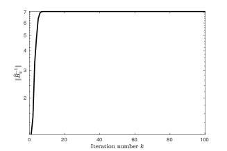
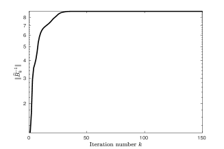
Second, in finite precision, we will show that the orthogonality levels of Uk+1subscript𝑈𝑘1U_{k+1}, V~ksubscript~𝑉𝑘\widetilde{V}_{k} and U^ksubscript^𝑈𝑘\widehat{U}_{k} are closely related and those of V^ksubscript^𝑉𝑘\widehat{V}_{k} and Vksubscript𝑉𝑘V_{k} interact too. In particular, we derive an upper bound for the orthogonality level of U^ksubscript^𝑈𝑘\widehat{U}_{k}, which is shown to be controlled by not only the orthogonality levels of V~ksubscript~𝑉𝑘\widetilde{V}_{k} and Uk+1subscript𝑈𝑘1{U}_{k+1} but also a gradually growing quantity B^k1normsuperscriptsubscript^𝐵𝑘1\|\widehat{B}_{k}^{-1}\|. The result indicates that the orthogonality level of U^ksubscript^𝑈𝑘\widehat{U}_{k} is similar to those of Uk+1subscript𝑈𝑘1U_{k+1} and V~ksubscript~𝑉𝑘\widetilde{V}_{k}, provided that B^ksubscript^𝐵𝑘\widehat{B}_{k} is not ill conditioned. Therefore, when designing a reorthogonalization strategy for the JBD process, one reorthogonalizes only uisubscript𝑢𝑖u_{i} and v~isubscript~𝑣𝑖\tilde{v}_{i} but u^isubscript^𝑢𝑖\hat{u}_{i}, which can save considerable reorthogonalization work.

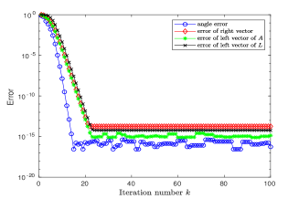
Third, we shall show how to make use of the JBD process to compute extreme GSVD components of {A,L}𝐴𝐿\{A,L\}, leading to the JBD method for the large GSVD computation. Precisely, we will propose three approaches to compute approximate generalized singular values and approximate right generalized singular vectors by exploiting the SVDs of Bksubscript𝐵𝑘B_{k} and B¯ksubscript¯𝐵𝑘\bar{B}_{k} and the GSVD of {Bk,B¯k}subscript𝐵𝑘subscript¯𝐵𝑘\{B_{k},\bar{B}_{k}\}, respectively; we will present two approaches to compute approximate left generalized singular vectors of A𝐴A and L𝐿L via either the left singular vectors of Bksubscript𝐵𝑘B_{k} and B¯ksubscript¯𝐵𝑘\bar{B}_{k} simultaneously or the left generalized singular vectors of {Bk,B¯k}subscript𝐵𝑘subscript¯𝐵𝑘\{B_{k},\bar{B}_{k}\}. We will investigate the convergence of the approximate generalized singular values that are computed by the singular values of Bksubscript𝐵𝑘B_{k} or B¯ksubscript¯𝐵𝑘\bar{B}_{k}. Similarly to Lanczos bidiagonalization, the loss of orthogonality of Lanczos type vectors computed by the JBD process leads to a delay of the convergence of the computed Ritz values and the appearance of spurious copies. We show that, under the assumptions that Bk1normsuperscriptsubscript𝐵𝑘1\|B_{k}^{-1}\| and B^k1normsuperscriptsubscript^𝐵𝑘1\|\widehat{B}_{k}^{-1}\| are modest uniformly with k𝑘k, the semiorthogonality of Lanczos type vectors suffices to avoid spurious copies and guarantees that the approximate generalized singular values have the same accuracy as the full orthogonality does. Here the semiorthogonality means that the absolute value of inner product of two unit length vectors is at the level of O(ϵ1/2)𝑂superscriptitalic-ϵ12O(\epsilon^{1/2}), in contrast to the full orthogonality level O(ϵ)𝑂italic-ϵO(\epsilon). Therefore, the semiorthogonality of Lanczos vectors suffices for the JBD method. In the meantime, we study the residual norm of an approximate generalized singular value and approximate right generalized singular vector, whose size is used to design a stopping tolerance for the JBD method. In finite precision, we derive an upper bound for the residual norm, and show that this upper bound can replace the residual norm to design a reliable stopping criterion without explicitly computing approximate right generalized singular vectors before the convergence occurs. We only compute the approximate right generalized singular vectors by solving certain consistent least squares problems with the coefficient matrix (AT,LT)Tsuperscriptsuperscript𝐴𝑇superscript𝐿𝑇𝑇(A^{T},L^{T})^{T} at the convergence rather than doing so at each iteration.

The paper is organized as follows. In Section 2, we review the GSVD of {A,L}𝐴𝐿\{A,L\} and describe the JBD process in exact arithmetic. In Section 3, we make a numerical analysis of the JBD process in finite precision. We establish relationships between the JBD process and two lower and upper Lanczos bidiagonalizations, and investigate interactions of orthogonality levels of the computed Lanczos type vectors. In Section 4, we describe the JBD method for computing a number of extreme generalized singular values and vectors of {A,L}𝐴𝐿\{A,L\}, and discuss the convergence and stopping criteria. In Section 5, we report numerical experiments to confirm our results. Finally, we conclude the paper with some remarks and future work in Section 6.

Throughout the paper, we denote by Iksubscript𝐼𝑘I_{k} the identity matrix of order k𝑘k, by 0ksubscript0𝑘0_{k} and 0k×lsubscript0𝑘𝑙0_{k\times l} the k𝑘k-dimensional zero vector and the k×l𝑘𝑙k\times l zero matrix, respectively. The transpose of a matrix C𝐶C is denoted by CTsuperscript𝐶𝑇C^{T}, and \|\cdot\| is the 2-norm of a matrix.

2 GSVD and the JBD process

We describe the GSVD of {A,L}𝐴𝐿\{A,L\} and the JBD process with some of its basic properties. Let the compact QR factorization of (AT,LT)Tsuperscriptsuperscript𝐴𝑇superscript𝐿𝑇𝑇(A^{T},L^{T})^{T} be defined as (1) and

(6) QA=PACAWT,QL=PLSLWTformulae-sequencesubscript𝑄𝐴subscript𝑃𝐴subscript𝐶𝐴superscript𝑊𝑇subscript𝑄𝐿subscript𝑃𝐿subscript𝑆𝐿superscript𝑊𝑇Q_{A}=P_{A}C_{A}W^{T},\ \ Q_{L}=P_{L}S_{L}W^{T}

be the CS decomposition of the matrix pair {QA,QL}subscript𝑄𝐴subscript𝑄𝐿\{Q_{A},Q_{L}\} [5, §2.5.4], where PAm×msubscript𝑃𝐴superscript𝑚𝑚P_{A}\in\mathbb{R}^{m\times m}, PLp×psubscript𝑃𝐿superscript𝑝𝑝P_{L}\in\mathbb{R}^{p\times p} and Wn×n𝑊superscript𝑛𝑛W\in\mathbb{R}^{n\times n} are orthogonal matrices, and CAm×nsubscript𝐶𝐴superscript𝑚𝑛C_{A}\in\mathbb{R}^{m\times n} and SLp×nsubscript𝑆𝐿superscript𝑝𝑛S_{L}\in\mathbb{R}^{p\times n} are diagonal matrices (not necessarily square) satisfying CATCA+SLTSL=Insuperscriptsubscript𝐶𝐴𝑇subscript𝐶𝐴superscriptsubscript𝑆𝐿𝑇subscript𝑆𝐿subscript𝐼𝑛C_{A}^{T}C_{A}+S_{L}^{T}S_{L}=I_{n}.

Suppose that rank((AT,LT)T)=rranksuperscriptsuperscript𝐴𝑇superscript𝐿𝑇𝑇𝑟\mathop{\operator@font rank}\nolimits((A^{T},L^{T})^{T})=r. It is shown in [25] that CAsubscript𝐶𝐴C_{A} and SLsubscript𝑆𝐿S_{L} can be written as

CA=(ΣA,0mrnr),SL=(ΣL,0prnr),formulae-sequencesubscript𝐶𝐴fragmentsΣ𝐴,0𝑚fragmentsrfragmentsnrsubscript𝑆𝐿fragmentsΣ𝐿,0𝑝fragmentsrfragmentsnrC_{A}=\vtop{\hbox{$\left(\vbox{\vbox{\halign{ \hfil$#$\hfil\kern 2\p@\kern\@leftbwd& \thinspace\hfil$#$\hfil&& \quad\hfil$#$\hfil\cr\Sigma_{A},$\hfil\kern 2.0pt\kern 6.66669pt&0&m\crcr\kern 2.0pt\cr r$\hfil\kern 2.0pt\kern 6.66669pt&n-r\cr} }\kern-27.48329pt}\kern 0.0pt\right)\kern-6.66669pt\kern 0.0pt$}\kern 27.48329pt}\ ,\ \ \ \ S_{L}=\vtop{\hbox{$\left(\vbox{\vbox{\halign{ \hfil$#$\hfil\kern 2\p@\kern\@leftbwd& \thinspace\hfil$#$\hfil&& \quad\hfil$#$\hfil\cr\Sigma_{L},$\hfil\kern 2.0pt\kern 6.66669pt&0&p\crcr\kern 2.0pt\cr r$\hfil\kern 2.0pt\kern 6.66669pt&n-r\cr} }\kern-27.48329pt}\kern 0.0pt\right)\kern-6.66669pt\kern 0.0pt$}\kern 27.48329pt},

where

ΣA=(IqqCllOmqlqlrql),ΣL=(Opr+qSllItrqlqlrql).formulae-sequencesubscriptΣ𝐴fragmentsI𝑞missing-subexpressionmissing-subexpression𝑞fragmentsC𝑙missing-subexpression𝑙missing-subexpression𝑂fragmentsmqlfragmentsq𝑙fragmentsrqlsubscriptΣ𝐿fragmentsOmissing-subexpressionmissing-subexpressionfragmentsprqfragmentsS𝑙missing-subexpression𝑙missing-subexpressionfragmentsI𝑡fragmentsrqlfragmentsq𝑙fragmentsrql\Sigma_{A}=\vtop{\hbox{$\left(\vbox{\vbox{\halign{ \hfil$#$\hfil\kern 2\p@\kern\@leftbwd& \thinspace\hfil$#$\hfil&& \quad\hfil$#$\hfil\cr I_{q}$\hfil\kern 2.0pt\kern 6.66669pt&&&q\crcr\kern 2.0pt\cr$\hfil\kern 2.0pt\kern 6.66669pt&C_{l}&&l\cr$\hfil\kern 2.0pt\kern 6.66669pt&&O&m-q-l\cr q$\hfil\kern 2.0pt\kern 6.66669pt&l&r-q-l\crcr} }\kern-50.1944pt}\kern 0.0pt\right)\kern-6.66669pt\kern 0.0pt$}\kern 50.1944pt},\ \ \ \ \Sigma_{L}=\vtop{\hbox{$\left(\vbox{\vbox{\halign{ \hfil$#$\hfil\kern 2\p@\kern\@leftbwd& \thinspace\hfil$#$\hfil&& \quad\hfil$#$\hfil\cr O$\hfil\kern 2.0pt\kern 6.66669pt&&&p-r+q\crcr\kern 2.0pt\cr$\hfil\kern 2.0pt\kern 6.66669pt&S_{l}&&l\cr$\hfil\kern 2.0pt\kern 6.66669pt&&I_{t}&r-q-l\cr q$\hfil\kern 2.0pt\kern 6.66669pt&l&r-q-l\crcr} }\kern-49.8444pt}\kern 0.0pt\right)\kern-6.66669pt\kern 0.0pt$}\kern 49.8444pt}.

Write Cl=diag(cq+1,,cq+l)subscript𝐶𝑙diagsubscript𝑐𝑞1subscript𝑐𝑞𝑙C_{l}=\mathop{\operator@font diag}\nolimits(c_{q+1},\dots,c_{q+l}),  cq+1cq+l>0subscript𝑐𝑞1subscript𝑐𝑞𝑙0c_{q+1}\geq\cdots\geq c_{q+l}>0 and Sl=diag(sq+1,,sq+l)subscript𝑆𝑙diagsubscript𝑠𝑞1subscript𝑠𝑞𝑙S_{l}=\mathop{\operator@font diag}\nolimits(s_{q+1},\dots,s_{q+l}),  0<sq+1sq+l0subscript𝑠𝑞1subscript𝑠𝑞𝑙0<s_{q+1}\leq\cdots\leq s_{q+l}. Then ci2+si2=1,i=q+1,,q+lformulae-sequencesuperscriptsubscript𝑐𝑖2superscriptsubscript𝑠𝑖21𝑖𝑞1𝑞𝑙c_{i}^{2}+s_{i}^{2}=1,\ i=q+1,\dots,q+l, and the generalized singular values of {A,L}𝐴𝐿\{A,L\} are

,,q,cq+1/sq+1,,cq+l/sq+ll,0,,0t,subscript𝑞subscriptsubscript𝑐𝑞1subscript𝑠𝑞1subscript𝑐𝑞𝑙subscript𝑠𝑞𝑙𝑙subscript00𝑡\underbrace{\infty,\dots,\infty}_{q},\ \ \underbrace{c_{q+1}/s_{q+1},\dots,c_{q+l}/s_{q+l}}_{l},\ \ \underbrace{0,\dots,0}_{t},

where t=rql𝑡𝑟𝑞𝑙t=r-q-l.

To ease the presentation, in the sequel, we always assume that {A,L}𝐴𝐿\{A,L\} is regular. Then R𝑅R in (1) is nonsingular and the GSVD of {A,L}𝐴𝐿\{A,L\} is

(7) A=PACAX1,L=PLSLX1formulae-sequence𝐴subscript𝑃𝐴subscript𝐶𝐴superscript𝑋1𝐿subscript𝑃𝐿subscript𝑆𝐿superscript𝑋1A=P_{A}C_{A}X^{-1},\ \ L=P_{L}S_{L}X^{-1}

with X=R1Wn×n𝑋superscript𝑅1𝑊superscript𝑛𝑛X=R^{-1}W\in\mathbb{R}^{n\times n}. Let X=(x1,,xn)𝑋subscript𝑥1subscript𝑥𝑛X=(x_{1},\ldots,x_{n}), PA=(p1A,,pmA)subscript𝑃𝐴superscriptsubscript𝑝1𝐴superscriptsubscript𝑝𝑚𝐴P_{A}=(p_{1}^{A},\ldots,p_{m}^{A}) and PL=(p1L,,ppL)subscript𝑃𝐿superscriptsubscript𝑝1𝐿superscriptsubscript𝑝𝑝𝐿P_{L}=(p_{1}^{L},\ldots,p_{p}^{L}). We can write the GSVD (7) in the vector form:

(8) {Axi=cipiA,Lxi=sipiL,siATpiA=ciLTpiL,i=1,,n,\left\{\begin{aligned} Ax_{i}&=c_{i}p_{i}^{A},\\ Lx_{i}&=s_{i}p_{i}^{L},\\ s_{i}A^{T}p_{i}^{A}&=c_{i}L^{T}p_{i}^{L},\end{aligned}\right.\qquad i=1,\dots,n,

where the i𝑖i-th large generalized singular value of {A,L}𝐴𝐿\{A,L\} is ci/sisubscript𝑐𝑖subscript𝑠𝑖c_{i}/s_{i}, and the i𝑖i-th corresponding generalized singular vectors are xisubscript𝑥𝑖x_{i}, piAsubscriptsuperscript𝑝𝐴𝑖p^{A}_{i} and piLsuperscriptsubscript𝑝𝑖𝐿p_{i}^{L}, respectively. We call xisubscript𝑥𝑖x_{i} the right generalized singular vector, piAsubscriptsuperscript𝑝𝐴𝑖p^{A}_{i} and piLsuperscriptsubscript𝑝𝑖𝐿p_{i}^{L} the left generalized singular vectors corresponding to ci/sisubscript𝑐𝑖subscript𝑠𝑖c_{i}/s_{i}. Since ci/si=subscript𝑐𝑖subscript𝑠𝑖c_{i}/s_{i}=\infty and ci/si=0subscript𝑐𝑖subscript𝑠𝑖0c_{i}/s_{i}=0 when si=0subscript𝑠𝑖0s_{i}=0 and si=1subscript𝑠𝑖1s_{i}=1, it is more convenient to use pair {ci,si}subscript𝑐𝑖subscript𝑠𝑖\{c_{i},s_{i}\} to denote ci/sisubscript𝑐𝑖subscript𝑠𝑖c_{i}/s_{i}. We also note that each xisubscript𝑥𝑖x_{i} satisfies the normalization xiT(ATA+LTL)xi=1superscriptsubscript𝑥𝑖𝑇superscript𝐴𝑇𝐴superscript𝐿𝑇𝐿subscript𝑥𝑖1x_{i}^{T}(A^{T}A+L^{T}L)x_{i}=1.

We describe the JBD process [16] as Algorithm 1, which, in exact arithmetic, corresponds to the lower and upper Lanczos bidiagonalization of QAsubscript𝑄𝐴Q_{A} and QLsubscript𝑄𝐿Q_{L}, respectively:

(9) QAVk=Uk+1Bk,QATUk+1=VkBkT+αk+1vk+1ek+1T,formulae-sequencesubscript𝑄𝐴subscript𝑉𝑘subscript𝑈𝑘1subscript𝐵𝑘superscriptsubscript𝑄𝐴𝑇subscript𝑈𝑘1subscript𝑉𝑘superscriptsubscript𝐵𝑘𝑇subscript𝛼𝑘1subscript𝑣𝑘1superscriptsubscript𝑒𝑘1𝑇\displaystyle Q_{A}V_{k}=U_{k+1}B_{k},\ \ Q_{A}^{T}U_{k+1}=V_{k}B_{k}^{T}+\alpha_{k+1}v_{k+1}e_{k+1}^{T},
(10) QLV^k=U^kB^k,QLTU^k=V^kB^kT+β^kv^k+1ekTformulae-sequencesubscript𝑄𝐿subscript^𝑉𝑘subscript^𝑈𝑘subscript^𝐵𝑘superscriptsubscript𝑄𝐿𝑇subscript^𝑈𝑘subscript^𝑉𝑘superscriptsubscript^𝐵𝑘𝑇subscript^𝛽𝑘subscript^𝑣𝑘1superscriptsubscript𝑒𝑘𝑇\displaystyle Q_{L}\widehat{V}_{k}=\widehat{U}_{k}\widehat{B}_{k},\ \ Q_{L}^{T}\widehat{U}_{k}=\widehat{V}_{k}\widehat{B}_{k}^{T}+\hat{\beta}_{k}\hat{v}_{k+1}e_{k}^{T}

with v^1=v1subscript^𝑣1subscript𝑣1\hat{v}_{1}=v_{1}, where eksubscript𝑒𝑘e_{k} is the last column of Iksubscript𝐼𝑘I_{k}, which are k𝑘k-step lower and upper Lanczos bidiagonalization processes of QAsubscript𝑄𝐴Q_{A} and QLsubscript𝑄𝐿Q_{L}, respectively.

Algorithm 1 The k𝑘k-step JBD process
1:  Choose a nonzero starting vector bm𝑏superscript𝑚b\in\mathbb{R}^{m}, and let β1u1=b,β1=bformulae-sequencesubscript𝛽1subscript𝑢1𝑏subscript𝛽1norm𝑏\beta_{1}u_{1}=b,\ \beta_{1}=\|b\|
2:  α1v~1=QQT(u10p)subscript𝛼1subscript~𝑣1𝑄superscript𝑄𝑇matrixsubscript𝑢1subscript0𝑝\alpha_{1}\tilde{v}_{1}=QQ^{T}\begin{pmatrix}u_{1}\\ 0_{p}\end{pmatrix}
3:   α^1u^1=v~1(m+1:m+p)\hat{\alpha}_{1}\hat{u}_{1}=\tilde{v}_{1}(m+1:m+p)
4:  for i=1,2,,k,𝑖12𝑘i=1,2,\ldots,k, do
5:     βi+1ui+1=v~i(1:m)αiui\beta_{i+1}u_{i+1}=\tilde{v}_{i}(1:m)-\alpha_{i}u_{i}
6:     αi+1v~i+1=QQT(ui+10p)βi+1v~isubscript𝛼𝑖1subscript~𝑣𝑖1𝑄superscript𝑄𝑇matrixsubscript𝑢𝑖1subscript0𝑝subscript𝛽𝑖1subscript~𝑣𝑖\alpha_{i+1}\tilde{v}_{i+1}=QQ^{T}\begin{pmatrix}u_{i+1}\\ 0_{p}\end{pmatrix}-\beta_{i+1}\tilde{v}_{i}
7:     β^i=(αi+1βi+1)/α^isubscript^𝛽𝑖subscript𝛼𝑖1subscript𝛽𝑖1subscript^𝛼𝑖\hat{\beta}_{i}=(\alpha_{i+1}\beta_{i+1})/\hat{\alpha}_{i}
8:     α^i+1u^i+1=(1)iv~i+1(m+1:m+p)β^iu^i\hat{\alpha}_{i+1}\hat{u}_{i+1}=(-1)^{i}\tilde{v}_{i+1}(m+1:m+p)-\hat{\beta}_{i}\hat{u}_{i}
9:  end for

At each iteration i=1,2,,k𝑖12𝑘i=1,2,\ldots,k, Algorithm 1 needs to compute QQT(ui0p)𝑄superscript𝑄𝑇matrixsubscript𝑢𝑖subscript0𝑝QQ^{T}\begin{pmatrix}u_{i}\\ 0_{p}\end{pmatrix}. For A𝐴A and L𝐿L large, however, the compact QR factorization (1) of (AT,LT)Tsuperscriptsuperscript𝐴𝑇superscript𝐿𝑇𝑇(A^{T},L^{T})^{T} is generally impractical, that is, both Q𝑄Q and R𝑅R are not available. Let u~i=(ui0p)subscript~𝑢𝑖matrixsubscript𝑢𝑖subscript0𝑝\tilde{u}_{i}=\begin{pmatrix}u_{i}\\ 0_{p}\end{pmatrix}. Since QQTu~i𝑄superscript𝑄𝑇subscript~𝑢𝑖QQ^{T}\tilde{u}_{i} is nothing but the orthogonal projection of u~isubscript~𝑢𝑖\tilde{u}_{i} onto the column space of (AT,LT)Tsuperscriptsuperscript𝐴𝑇superscript𝐿𝑇𝑇(A^{T},L^{T})^{T}, we have QQTu~i=(AL)x~i𝑄superscript𝑄𝑇subscript~𝑢𝑖matrix𝐴𝐿subscript~𝑥𝑖QQ^{T}\tilde{u}_{i}=\begin{pmatrix}A\\ L\end{pmatrix}\tilde{x}_{i}, where

(11) x~i=argminx~n(AL)x~u~i.subscript~𝑥𝑖subscript~𝑥superscript𝑛normmatrix𝐴𝐿~𝑥subscript~𝑢𝑖\tilde{x}_{i}=\arg\min_{\tilde{x}\in\mathbb{R}^{n}}\left\|\begin{pmatrix}A\\ L\end{pmatrix}\tilde{x}-\tilde{u}_{i}\right\|.

This large scale least squares problem can be solved by an iterative solver, e.g., the most commonly used LSQR algorithm [26].

In exact arithmetic, the k𝑘k-step JBD process produces the two bidiagonal matrices Bksubscript𝐵𝑘B_{k}, B^ksubscript^𝐵𝑘\widehat{B}_{k} and three orthonormal matrices Uk+1subscript𝑈𝑘1U_{k+1}, U^ksubscript^𝑈𝑘\widehat{U}_{k} in (3)–(4) and

(12) V~k=(v~1,,v~k)(m+p)×k,subscript~𝑉𝑘subscript~𝑣1subscript~𝑣𝑘superscript𝑚𝑝𝑘\displaystyle\widetilde{V}_{k}=(\tilde{v}_{1},\ldots,\tilde{v}_{k})\in\mathbb{R}^{(m+p)\times k},

where v~i=Qvisubscript~𝑣𝑖𝑄subscript𝑣𝑖\tilde{v}_{i}=Qv_{i} with visubscript𝑣𝑖v_{i} the i𝑖i-th column of Vksubscript𝑉𝑘V_{k} in (3), i.e., vi=QTv~isubscript𝑣𝑖superscript𝑄𝑇subscript~𝑣𝑖v_{i}=Q^{T}\tilde{v}_{i}. It can be written as

(13) (Im,0m×p)V~k=Uk+1Bk,subscript𝐼𝑚subscript0𝑚𝑝subscript~𝑉𝑘subscript𝑈𝑘1subscript𝐵𝑘\displaystyle(I_{m},0_{m\times p})\widetilde{V}_{k}=U_{k+1}B_{k},
(14) QQT(Uk+10p×(k+1))=V~kBkT+αk+1v~k+1ek+1T,𝑄superscript𝑄𝑇matrixsubscript𝑈𝑘1subscript0𝑝𝑘1subscript~𝑉𝑘superscriptsubscript𝐵𝑘𝑇subscript𝛼𝑘1subscript~𝑣𝑘1superscriptsubscript𝑒𝑘1𝑇\displaystyle QQ^{T}\begin{pmatrix}U_{k+1}\\ 0_{p\times(k+1)}\end{pmatrix}=\widetilde{V}_{k}B_{k}^{T}+\alpha_{k+1}\tilde{v}_{k+1}e_{k+1}^{T},
(15) (0p×m,Ip)V~kDk=U^kB^k,subscript0𝑝𝑚subscript𝐼𝑝subscript~𝑉𝑘subscript𝐷𝑘subscript^𝑈𝑘subscript^𝐵𝑘\displaystyle(0_{p\times m},I_{p})\widetilde{V}_{k}D_{k}=\widehat{U}_{k}\widehat{B}_{k},

where Dk=diag(1,1,,(1)k1)k×ksubscript𝐷𝑘diag11superscript1𝑘1superscript𝑘𝑘D_{k}=\mathop{\operator@font diag}\nolimits(1,-1,\dots,(-1)^{k-1})\in\mathbb{R}^{k\times k}, and ek+1subscript𝑒𝑘1e_{k+1} is the last column of Ik+1subscript𝐼𝑘1I_{k+1}.

It is shown [16] that, in exact arithmetic, the k𝑘k-step JBD process satisfies

(16) AZk=Uk+1Bk,LZk=U^kB¯k,formulae-sequence𝐴subscript𝑍𝑘subscript𝑈𝑘1subscript𝐵𝑘𝐿subscript𝑍𝑘subscript^𝑈𝑘subscript¯𝐵𝑘AZ_{k}=U_{k+1}B_{k},\ \ LZ_{k}=\widehat{U}_{k}\bar{B}_{k},

where Zk=R1Vk=(z1,,zk)subscript𝑍𝑘superscript𝑅1subscript𝑉𝑘subscript𝑧1subscript𝑧𝑘Z_{k}=R^{-1}V_{k}=(z_{1},\dots,z_{k}) and B¯k=B^kDksubscript¯𝐵𝑘subscript^𝐵𝑘subscript𝐷𝑘\bar{B}_{k}=\widehat{B}_{k}D_{k}, and

(17) BkTBk+B¯kTB¯k=Ik.superscriptsubscript𝐵𝑘𝑇subscript𝐵𝑘superscriptsubscript¯𝐵𝑘𝑇subscript¯𝐵𝑘subscript𝐼𝑘B_{k}^{T}B_{k}+\bar{B}_{k}^{T}\bar{B}_{k}=I_{k}.

Therefore, the singular values of Bksubscript𝐵𝑘B_{k} are determined by those of B¯ksubscript¯𝐵𝑘\bar{B}_{k}, i.e., B^ksubscript^𝐵𝑘\widehat{B}_{k}, and vice versa. As a result, if some extreme generalized singular values of {A,L}𝐴𝐿\{A,L\} are of interest, one can use the extreme generalized singular values of {Bk,B¯k}subscript𝐵𝑘subscript¯𝐵𝑘\{B_{k},\bar{B}_{k}\} to approximate them by either computing the generalized singular values of the small pairs or only computing the singular values of Bksubscript𝐵𝑘B_{k} or B¯ksubscript¯𝐵𝑘\bar{B}_{k}.

In finite precision, it is well known that the Lanczos vectors computed by Lanczos bidiagonalization gradually lose their mutual orthogonality as the iteration number k𝑘k increases [18]. Following [18, 32], we define the orthogonality level of a set of vectors as follows.

Definition 2.1.

For a rectangular matrix Wk=(w1,,wk)r×ksubscript𝑊𝑘subscript𝑤1subscript𝑤𝑘superscript𝑟𝑘W_{k}=(w_{1},\dots,w_{k})\in\mathbb{R}^{r\times k} with wj=1\lVert w_{j}\lVert=1, j=1,,k𝑗1𝑘j=1,\dots,k, we call ξijw=|wiTwj|superscriptsubscript𝜉𝑖𝑗𝑤superscriptsubscript𝑤𝑖𝑇subscript𝑤𝑗\xi_{ij}^{w}=|w_{i}^{T}w_{j}| the orthogonality level among wisubscript𝑤𝑖w_{i} and wjsubscript𝑤𝑗w_{j}. The orthogonality level of {w1,,wk}subscript𝑤1subscript𝑤𝑘\{w_{1},\dots,w_{k}\} or Wksubscript𝑊𝑘W_{k} is measured by one of

(18) ξ(Wk)=max1ijkξijw,𝜉subscript𝑊𝑘subscript1𝑖𝑗𝑘superscriptsubscript𝜉𝑖𝑗𝑤\displaystyle\xi(W_{k})=\max_{1\leq i\neq j\leq k}\xi_{ij}^{w},
(19) η(Wk)=IkWkTWk.𝜂subscript𝑊𝑘normsubscript𝐼𝑘superscriptsubscript𝑊𝑘𝑇subscript𝑊𝑘\displaystyle\eta(W_{k})=\|I_{k}-W_{k}^{T}W_{k}\|.

Notice that ξ(Wk)η(Wk)kξ(Wk)𝜉subscript𝑊𝑘𝜂subscript𝑊𝑘𝑘𝜉subscript𝑊𝑘\xi(W_{k})\leq\eta(W_{k})\leq k\xi(W_{k}). The above two quantities can be used interchangeably to measure the orthogonality level of Lanczos vectors. Let σi()subscript𝜎𝑖\sigma_{i}(\cdot) and λi()subscript𝜆𝑖\lambda_{i}(\cdot) be the i𝑖i-th largest singular value and eigenvalue of a symmetric matrix respectively. Then

σ12(Wk)=λ1(WkTWk)=1+λ1(WkTWkIk)1+IkWkTWk,\sigma_{1}^{2}(W_{k})=\lambda_{1}(W_{k}^{T}W_{k})=1+\lambda_{1}(W_{k}^{T}W_{k}-I_{k})\leq 1+\lVert I_{k}-W_{k}^{T}W_{k}\lVert,

which leads to

(20) Wk1+η(Wk).normsubscript𝑊𝑘1𝜂subscript𝑊𝑘\|W_{k}\|\leq\sqrt{1+\eta(W_{k})}.

For Lanczos bidiagonalization, the loss of orthogonality of the Lanczos vectors will lead to appearance of spurious Ritz values and a delay of the convergence of Ritz values [18]. Therefore, reorthogonalization strategies are necessary to maintain necessary orthogonality level in order to preserve convergence of Ritz values and avoid spurious copies; see [1, 18, 28, 30, 31, 32] for a few types of reorthogonalization strategies and related analysis.

3 The JBD process in finite precision

When it is carried out in finite precision, due to the influence of rounding errors, the behavior of the JBD process will deviate from that in exact arithmetic. First, the JBD process of {A,L}𝐴𝐿\{A,L\} is not equivalent to the combination of the two Lanczos bidiagonalizations any longer. Second, the three matrices Uk+1subscript𝑈𝑘1U_{k+1}, V~ksubscript~𝑉𝑘\widetilde{V}_{k} and U^ksubscript^𝑈𝑘\widehat{U}_{k} lose their numerical orthogonality gradually as k𝑘k increases. In this paper, we do not consider the solution accuracy of the inner least squares problem (11) at each iteration, though it has an important influence on the accuracy and efficiency of the algorithm. This issue is complicated, and we will study it in our future work. In the following analysis, we always assume that (11) is solved accurately, i.e., (AL)x~i=QQT(ui0p)matrix𝐴𝐿subscript~𝑥𝑖𝑄superscript𝑄𝑇matrixsubscript𝑢𝑖subscript0𝑝\begin{pmatrix}A\\ L\end{pmatrix}\tilde{x}_{i}=QQ^{T}\begin{pmatrix}u_{i}\\ 0_{p}\end{pmatrix}.

First of all, we state a set of basics and assumptions on the behavior of the rounding errors occurring in the JBD process. They are adapted from the symmetric Lanczos process and Lanczos bidiagonalization, constitute a model for the actual computation, and grasp essential features but discard those irrelevant or negligible ones. From now on, without confusion, we use the same notation as before to denote the computed ones in finite precision. In this case, relations (13)–(15) add rounding error terms (cf. [27, §13.4]) and become

(21) (Im,0m×p)V~k=Uk+1Bk+F~k,subscript𝐼𝑚subscript0𝑚𝑝subscript~𝑉𝑘subscript𝑈𝑘1subscript𝐵𝑘subscript~𝐹𝑘\displaystyle(I_{m},0_{m\times p})\widetilde{V}_{k}=U_{k+1}B_{k}+\widetilde{F}_{k},
(22) QQT(Uk+10p×(k+1))=V~kBkT+αk+1v~k+1ek+1T+G~k+1,𝑄superscript𝑄𝑇matrixsubscript𝑈𝑘1subscript0𝑝𝑘1subscript~𝑉𝑘superscriptsubscript𝐵𝑘𝑇subscript𝛼𝑘1subscript~𝑣𝑘1superscriptsubscript𝑒𝑘1𝑇subscript~𝐺𝑘1\displaystyle QQ^{T}\begin{pmatrix}U_{k+1}\\ 0_{p\times(k+1)}\end{pmatrix}=\widetilde{V}_{k}B_{k}^{T}+\alpha_{k+1}\tilde{v}_{k+1}e_{k+1}^{T}+\widetilde{G}_{k+1},
(23) (0p×m,Ip)V~kDk=U^kB^k+F¯k,subscript0𝑝𝑚subscript𝐼𝑝subscript~𝑉𝑘subscript𝐷𝑘subscript^𝑈𝑘subscript^𝐵𝑘subscript¯𝐹𝑘\displaystyle(0_{p\times m},I_{p})\widetilde{V}_{k}D_{k}=\widehat{U}_{k}\widehat{B}_{k}+\bar{F}_{k},

where the rounding error matrices F~k=(f~1,,f~k),G~k+1=(g~1,,g~k+1)formulae-sequencesubscript~𝐹𝑘subscript~𝑓1subscript~𝑓𝑘subscript~𝐺𝑘1subscript~𝑔1subscript~𝑔𝑘1\widetilde{F}_{k}=(\tilde{f}_{1},\dots,\tilde{f}_{k}),\ \widetilde{G}_{k+1}=(\tilde{g}_{1},\dots,\tilde{g}_{k+1}) and F¯k=(f¯1,,f¯k)subscript¯𝐹𝑘subscript¯𝑓1subscript¯𝑓𝑘\bar{F}_{k}=(\bar{f}_{1},\dots,\bar{f}_{k}) satisfy

(24) F~k,G~k+1,F¯k=O(ϵ).normsubscript~𝐹𝑘normsubscript~𝐺𝑘1normsubscript¯𝐹𝑘𝑂italic-ϵ\|\widetilde{F}_{k}\|,\|\widetilde{G}_{k+1}\|,\|\bar{F}_{k}\|=O(\epsilon).

Second, the following local orthogonality of uisubscript𝑢𝑖u_{i} and u^isubscript^𝑢𝑖\hat{u}_{i} holds [23, 30]:

(25) βi+1|ui+1Tui|=O(c1(m,n)ϵ),subscript𝛽𝑖1superscriptsubscript𝑢𝑖1𝑇subscript𝑢𝑖𝑂subscript𝑐1𝑚𝑛italic-ϵ\displaystyle\beta_{i+1}|u_{i+1}^{T}u_{i}|=O(c_{1}(m,n)\epsilon),
(26) α^i+1|u^i+1Tu^i|=O(c2(p,n)ϵ),subscript^𝛼𝑖1superscriptsubscript^𝑢𝑖1𝑇subscript^𝑢𝑖𝑂subscript𝑐2𝑝𝑛italic-ϵ\displaystyle\hat{\alpha}_{i+1}|\hat{u}_{i+1}^{T}\hat{u}_{i}|=O(c_{2}(p,n)\epsilon),

where c1(m,n)subscript𝑐1𝑚𝑛c_{1}(m,n) and c2(p,n)subscript𝑐2𝑝𝑛c_{2}(p,n) are modest constants depending on m𝑚m, n𝑛n and p𝑝p. Third, we assume that

(27) neitherβi+1norα^i+1everbecomesnegligible,𝑛𝑒𝑖𝑡𝑒𝑟subscript𝛽𝑖1𝑛𝑜𝑟subscript^𝛼𝑖1𝑒𝑣𝑒𝑟𝑏𝑒𝑐𝑜𝑚𝑒𝑠𝑛𝑒𝑔𝑙𝑖𝑔𝑖𝑏𝑙𝑒neither\ \ \beta_{i+1}\ nor\ \hat{\alpha}_{i+1}\ ever\ becomes\ negligible,

which is almost always true in practice. In case either βi+1subscript𝛽𝑖1\beta_{i+1} or α^i+1subscript^𝛼𝑖1\hat{\alpha}_{i+1} becomes negligible, the JBD process should be terminated since it has found either acceptable approximate right invariant generalized singular subspace and left generalized singular subspace for A𝐴A or acceptable approximate right invariant generalized singular subspace and left generalized singular subspace for L𝐿L, as can be justified from (9), (10) and (16). This can also be seen from the later Theorem 8 and α^iβ^i=αi+1βi+1subscript^𝛼𝑖subscript^𝛽𝑖subscript𝛼𝑖1subscript𝛽𝑖1\hat{\alpha}_{i}\hat{\beta}_{i}=\alpha_{i+1}\beta_{i+1} in step 7 of Algorithm 1. Finally, for simplicity, in our numerical analysis, we always assume that the computed Lanczos type vectors are of unit length.

3.1 Relationships between the JBD process and Lanczos bidiagonalization in finite precision

We show that, in finite precision, the JBD process of {A,L}𝐴𝐿\{A,L\} is no longer equivalent to the combination of the lower and upper Lanczos bidiagonalizations of QAsubscript𝑄𝐴Q_{A} and QLsubscript𝑄𝐿Q_{L}. To this end, we first present the following lemma.

Lemma 3.1.

Let vi=QTv~isubscript𝑣𝑖superscript𝑄𝑇subscript~𝑣𝑖v_{i}=Q^{T}\tilde{v}_{i}, Vk=(v1,,vk)subscript𝑉𝑘subscript𝑣1subscript𝑣𝑘V_{k}=(v_{1},\dots,v_{k}) and B¯k=(Bk1TαkekT)k×ksubscript¯𝐵𝑘matrixsuperscriptsubscript𝐵𝑘1𝑇subscript𝛼𝑘superscriptsubscript𝑒𝑘𝑇superscript𝑘𝑘\underline{B}_{k}=\begin{pmatrix}B_{k-1}^{T}\\ \alpha_{k}e_{k}^{T}\end{pmatrix}\in\mathbb{R}^{k\times k}. Then

(28) V~kQVkG~kB¯k1=O(B¯k1ϵ)\lVert\widetilde{V}_{k}-QV_{k}\lVert\leq\lVert\widetilde{G}_{k}\underline{B}_{k}^{-1}\lVert=O(\lVert\underline{B}_{k}^{-1}\lVert\epsilon)

with G~ksubscript~𝐺𝑘\widetilde{G}_{k} defined in (22).

Proof.

Write the matrix C=(AT,LT)T𝐶superscriptsuperscript𝐴𝑇superscript𝐿𝑇𝑇C=(A^{T},L^{T})^{T}. Then

QQT=CC,QQTC=C,QQT(Uk0p×k)=CXk,formulae-sequence𝑄superscript𝑄𝑇𝐶superscript𝐶formulae-sequence𝑄superscript𝑄𝑇𝐶𝐶𝑄superscript𝑄𝑇matrixsubscript𝑈𝑘subscript0𝑝𝑘𝐶subscript𝑋𝑘QQ^{T}=CC^{{\dagger}},\ QQ^{T}C=C,\ QQ^{T}\begin{pmatrix}U_{k}\\ 0_{p\times k}\end{pmatrix}=CX_{k},

where ``"``"``{\dagger}" denotes the Moore–Penrose inverse of a matrix and Xk=C(Uk0p×k)subscript𝑋𝑘superscript𝐶matrixsubscript𝑈𝑘subscript0𝑝𝑘X_{k}=C^{{\dagger}}\begin{pmatrix}U_{k}\\ 0_{p\times k}\end{pmatrix}. From (22) and Vk=QTV~ksubscript𝑉𝑘superscript𝑄𝑇subscript~𝑉𝑘V_{k}=Q^{T}\widetilde{V}_{k}, we have CXk=V~kB¯k+G~k𝐶subscript𝑋𝑘subscript~𝑉𝑘subscript¯𝐵𝑘subscript~𝐺𝑘CX_{k}=\widetilde{V}_{k}\underline{B}_{k}+\widetilde{G}_{k}, leading to V~k=CXkB¯k1G~kB¯k1subscript~𝑉𝑘𝐶subscript𝑋𝑘superscriptsubscript¯𝐵𝑘1subscript~𝐺𝑘superscriptsubscript¯𝐵𝑘1\widetilde{V}_{k}=CX_{k}\underline{B}_{k}^{-1}-\widetilde{G}_{k}\underline{B}_{k}^{-1}. Therefore, we obtain

(29) V~kQVksubscript~𝑉𝑘𝑄subscript𝑉𝑘\displaystyle\widetilde{V}_{k}-QV_{k} =\displaystyle= V~kQQTV~k=V~kQQT(CXkB¯k1G~kB¯k1)subscript~𝑉𝑘𝑄superscript𝑄𝑇subscript~𝑉𝑘subscript~𝑉𝑘𝑄superscript𝑄𝑇𝐶subscript𝑋𝑘superscriptsubscript¯𝐵𝑘1subscript~𝐺𝑘superscriptsubscript¯𝐵𝑘1\displaystyle\widetilde{V}_{k}-QQ^{T}\widetilde{V}_{k}=\widetilde{V}_{k}-QQ^{T}(CX_{k}\underline{B}_{k}^{-1}-\widetilde{G}_{k}\underline{B}_{k}^{-1})
=\displaystyle= V~kCXkB¯k1+QQTG~kB¯k1=G~kB¯k1+QQTG~kB¯k1subscript~𝑉𝑘𝐶subscript𝑋𝑘superscriptsubscript¯𝐵𝑘1𝑄superscript𝑄𝑇subscript~𝐺𝑘superscriptsubscript¯𝐵𝑘1subscript~𝐺𝑘superscriptsubscript¯𝐵𝑘1𝑄superscript𝑄𝑇subscript~𝐺𝑘superscriptsubscript¯𝐵𝑘1\displaystyle\widetilde{V}_{k}-CX_{k}\underline{B}_{k}^{-1}+QQ^{T}\widetilde{G}_{k}\underline{B}_{k}^{-1}=-\widetilde{G}_{k}\underline{B}_{k}^{-1}+QQ^{T}\widetilde{G}_{k}\underline{B}_{k}^{-1}
=\displaystyle= (QQTIm+p)G~kB¯k1.𝑄superscript𝑄𝑇subscript𝐼𝑚𝑝subscript~𝐺𝑘superscriptsubscript¯𝐵𝑘1\displaystyle(QQ^{T}-I_{m+p})\widetilde{G}_{k}\underline{B}_{k}^{-1}.

Taking norms in both sides proves (28). ∎

This lemma shows that V~ksubscript~𝑉𝑘\widetilde{V}_{k} deviates from QVk𝑄subscript𝑉𝑘QV_{k} with the error O(B¯k1ϵ)O(\lVert\underline{B}_{k}^{-1}\lVert\epsilon) and V~k=QVksubscript~𝑉𝑘𝑄subscript𝑉𝑘\widetilde{V}_{k}=QV_{k} in exact arithmetic holds no longer. Using (28), we can rewrite (21) as

(30) (Im,0m×p)QVk=Uk+1Bk+Fksubscript𝐼𝑚subscript0𝑚𝑝𝑄subscript𝑉𝑘subscript𝑈𝑘1subscript𝐵𝑘subscript𝐹𝑘(I_{m},0_{m\times p})Q{V}_{k}=U_{k+1}B_{k}+F_{k}

where

(31) Fk=F~k(Im,0m×p)(V~kQVk).subscript𝐹𝑘subscript~𝐹𝑘subscript𝐼𝑚subscript0𝑚𝑝subscript~𝑉𝑘𝑄subscript𝑉𝑘F_{k}=\widetilde{F}_{k}-(I_{m},0_{m\times p})(\widetilde{V}_{k}-QV_{k}).

Then from (24) and (28) we have Fk=O(B¯k1ϵ)\|F_{k}\|=O(\lVert\underline{B}_{k}^{-1}\lVert\epsilon). Premultiplying (22) by QTsuperscript𝑄𝑇Q^{T} and exploiting (Im,0m×p)QVk=QAVksubscript𝐼𝑚subscript0𝑚𝑝𝑄subscript𝑉𝑘subscript𝑄𝐴subscript𝑉𝑘(I_{m},0_{m\times p})Q{V}_{k}=Q_{A}V_{k} straightforwardly yields the following result, which is the corresponding lower Lanczos bidiagonalization of QAsubscript𝑄𝐴Q_{A} in finite precision resulting from the JBD process.

Theorem 1.

Suppose that the inner least squares problem (11) is solved accurately. In finite precision, we have

(32) QAVk=Uk+1Bk+Fk,subscript𝑄𝐴subscript𝑉𝑘subscript𝑈𝑘1subscript𝐵𝑘subscript𝐹𝑘\displaystyle Q_{A}V_{k}=U_{k+1}B_{k}+F_{k},
(33) QATUk+1=VkBkT+αk+1vk+1ek+1T+Gk+1,superscriptsubscript𝑄𝐴𝑇subscript𝑈𝑘1subscript𝑉𝑘superscriptsubscript𝐵𝑘𝑇subscript𝛼𝑘1subscript𝑣𝑘1superscriptsubscript𝑒𝑘1𝑇subscript𝐺𝑘1\displaystyle Q_{A}^{T}U_{k+1}=V_{k}B_{k}^{T}+\alpha_{k+1}v_{k+1}e_{k+1}^{T}+G_{k+1},

where Gk+1=QTG~k+1subscript𝐺𝑘1superscript𝑄𝑇subscript~𝐺𝑘1G_{k+1}=Q^{T}\widetilde{G}_{k+1} with G~k+1subscript~𝐺𝑘1\widetilde{G}_{k+1} in (22) and Fk=O(B¯k1ϵ)\lVert F_{k}\lVert=O(\lVert\underline{B}_{k}^{-1}\lVert\epsilon), Gk+1=O(ϵ)\lVert G_{k+1}\lVert=O(\epsilon).

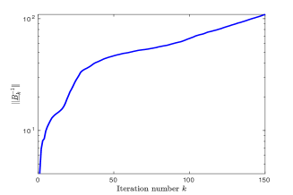
This theorem indicates that the error term Fksubscript𝐹𝑘F_{k} is amplified gradually once B¯k1\lVert\underline{B}_{k}^{-1}\lVert grows with k𝑘k. When QAsubscript𝑄𝐴Q_{A} is rectangular, i.e., m>n𝑚𝑛m>n, theoretically we cannot control the size of B¯k1normsuperscriptsubscript¯𝐵𝑘1\|\underline{B}_{k}^{-1}\|, as shown now: from the second relation in (9), we obtain

UkTQAQATUk=B¯kTB¯k,superscriptsubscript𝑈𝑘𝑇subscript𝑄𝐴superscriptsubscript𝑄𝐴𝑇subscript𝑈𝑘superscriptsubscript¯𝐵𝑘𝑇subscript¯𝐵𝑘U_{k}^{T}Q_{A}Q_{A}^{T}U_{k}=\underline{B}_{k}^{T}\underline{B}_{k},

indicating that the eigenvalues of B¯kTB¯ksuperscriptsubscript¯𝐵𝑘𝑇subscript¯𝐵𝑘\underline{B}_{k}^{T}\underline{B}_{k}, i.e., the squares of the singular values of B¯ksubscript¯𝐵𝑘\underline{B}_{k}, are the Ritz values of the singular matrix QAQATsubscript𝑄𝐴superscriptsubscript𝑄𝐴𝑇Q_{A}Q_{A}^{T} with respect to span(Uk)spansubscript𝑈𝑘{\rm span}(U_{k}) and lie between the largest and smallest eigenvalues of the singular matrix QAQATsubscript𝑄𝐴superscriptsubscript𝑄𝐴𝑇Q_{A}Q_{A}^{T}. Notice that span(Uk)spansubscript𝑈𝑘{\rm span}(U_{k}) is the Krylov subspace generated by u1,QAQATu1,,(QAQAT)k1u1subscript𝑢1subscript𝑄𝐴superscriptsubscript𝑄𝐴𝑇subscript𝑢1superscriptsubscript𝑄𝐴superscriptsubscript𝑄𝐴𝑇𝑘1subscript𝑢1u_{1},Q_{A}Q_{A}^{T}u_{1},\ldots,(Q_{A}Q_{A}^{T})^{k-1}u_{1}. Then that the smallest eigenvalue of B¯kTB¯ksuperscriptsubscript¯𝐵𝑘𝑇subscript¯𝐵𝑘\underline{B}_{k}^{T}\underline{B}_{k} converges to the zero eigenvalue of QAQATsubscript𝑄𝐴superscriptsubscript𝑄𝐴𝑇Q_{A}Q_{A}^{T} as k𝑘k increases, so that B¯k1normsuperscriptsubscript¯𝐵𝑘1\|\underline{B}_{k}^{-1}\| may become uncontrollably large; on the other hand, for QAsubscript𝑄𝐴Q_{A} flat or square, i.e., mn𝑚𝑛m\leq n, and having full row rank, however, such a phenomenon definitively cannot occur, and the smallest eigenvalue of B¯kTB¯ksuperscriptsubscript¯𝐵𝑘𝑇subscript¯𝐵𝑘\underline{B}_{k}^{T}\underline{B}_{k} is bounded from below by the smallest positive one of QAQATsubscript𝑄𝐴superscriptsubscript𝑄𝐴𝑇Q_{A}Q_{A}^{T}. In this case, B¯k1normsuperscriptsubscript¯𝐵𝑘1\|\underline{B}_{k}^{-1}\| is always uniformly bounded but possibly large when QAsubscript𝑄𝐴Q_{A} is ill conditioned. We refer the reader to [11] on a detailed analysis on B¯ksubscript¯𝐵𝑘\underline{B}_{k} and its singular values, which is closely related to and play a critical role in the conjugate gradient minimal error (CGME) method for solving least squares problems and linear discrete ill-posed problems. As a result, in finite precision, the the JBD process for computing Uk+1subscript𝑈𝑘1U_{k+1}, Vksubscript𝑉𝑘V_{k} and Bksubscript𝐵𝑘B_{k} may be no longer equivalent to the lower Lanczos bidiagonalization of QAsubscript𝑄𝐴Q_{A}, where the rounding error term in the place of Fksubscript𝐹𝑘F_{k} is O(QAϵ)=O(ϵ)𝑂normsubscript𝑄𝐴italic-ϵ𝑂italic-ϵO(\|Q_{A}\|\epsilon)=O(\epsilon) in size.

Similarly, from (5) and the first relation in (10) we have

VkTQLTQLVk=B¯kTB¯k.superscriptsubscript𝑉𝑘𝑇superscriptsubscript𝑄𝐿𝑇subscript𝑄𝐿subscript𝑉𝑘superscriptsubscript¯𝐵𝑘𝑇subscript¯𝐵𝑘V_{k}^{T}Q_{L}^{T}Q_{L}V_{k}=\bar{B}_{k}^{T}\bar{B}_{k}.

Since span(Vk)spansubscript𝑉𝑘{\rm span}(V_{k}) is the Krylov subspace generated by v1,QLTQLv1,,(QLTQL)k1v1subscript𝑣1superscriptsubscript𝑄𝐿𝑇subscript𝑄𝐿subscript𝑣1superscriptsuperscriptsubscript𝑄𝐿𝑇subscript𝑄𝐿𝑘1subscript𝑣1v_{1},Q_{L}^{T}Q_{L}v_{1},\ldots,(Q_{L}^{T}Q_{L})^{k-1}v_{1}, we can make a similar analysis to the above. Specifically, if QLsubscript𝑄𝐿Q_{L} is rectangular or square and of full column rank, then the smallest singular value of B¯ksubscript¯𝐵𝑘\bar{B}_{k} converges to the smallest one of QLsubscript𝑄𝐿Q_{L} from above as k𝑘k increases, and it is bounded from below by it, meaning that B¯k1normsuperscriptsubscript¯𝐵𝑘1\|\bar{B}_{k}^{-1}\| is controllable; if QLsubscript𝑄𝐿Q_{L} is flat, then the smallest singular value of B¯ksubscript¯𝐵𝑘\bar{B}_{k} converges to zero as k𝑘k increases, causing that B¯k1normsuperscriptsubscript¯𝐵𝑘1\|\bar{B}_{k}^{-1}\| cannot be controlled and become large as k𝑘k increases.

Note that the orders of QAsubscript𝑄𝐴Q_{A} and QLsubscript𝑄𝐿Q_{L} are the same as those of A𝐴A and L𝐿L, respectively. The above analysis and assertions suggest us to first check the orders of A𝐴A and L𝐿L and then perform the JBD process on either {A,L}𝐴𝐿\{A,L\} or {L,A}𝐿𝐴\{L,A\} when attempting to ensure that the resulting B¯k1\lVert\underline{B}_{k}^{-1}\lVert and B¯k1normsuperscriptsubscript¯𝐵𝑘1\|\bar{B}_{k}^{-1}\| are bounded whenever possible. As will be seen later, their boundedness is desirable for the JBD process and the JBD method for the GSVD computation in finite precision.

In finite precision, we next prove that relation (17) holds within O(ϵ)𝑂italic-ϵO(\epsilon), which is important to design an efficient and reliable algorithm for the GSVD computation. To this end, we first establish upper bounds for Bknormsubscript𝐵𝑘\|B_{k}\| and B^knormsubscript^𝐵𝑘\|\widehat{B}_{k}\|. From (21) and (23), at the i𝑖i-th step we have

(34) v~i(1:m)=αiui+βi+1ui+1+f~i,\displaystyle\tilde{v}_{i}(1:m)=\alpha_{i}u_{i}+\beta_{i+1}u_{i+1}+\tilde{f}_{i},
(35) (1)i1v~i(m+1:m+p)=α^iu^i+β^i1u^i1+f¯i.\displaystyle(-1)^{i-1}\tilde{v}_{i}(m+1:m+p)=\hat{\alpha}_{i}\hat{u}_{i}+\hat{\beta}_{i-1}\hat{u}_{i-1}+\bar{f}_{i}.

Thus αiui+βi+1ui+12=v~i(1:m)f~i2\|\alpha_{i}u_{i}+\beta_{i+1}u_{i+1}\|^{2}=\|\tilde{v}_{i}(1:m)-\tilde{f}_{i}\|^{2}, which leads to

(36) αi2+βi+12=v~i(1:m)2+f~i22f~iTv~i(1:m)2αiβi+1ui+1Tui1+O(c1(m,n)ϵ),\displaystyle\begin{split}\alpha_{i}^{2}+\beta_{i+1}^{2}&=\|\tilde{v}_{i}(1:m)\|^{2}+\|\tilde{f}_{i}\|^{2}-2\tilde{f}_{i}^{T}\tilde{v}_{i}(1:m)-2\alpha_{i}\beta_{i+1}u_{i+1}^{T}u_{i}\\ &\leq 1+O(c_{1}(m,n)\epsilon),\end{split}

where we have used (25). Similarly, we obtain

(37) α^i2+β^i121+O(c2(p,n)ϵ).superscriptsubscript^𝛼𝑖2superscriptsubscript^𝛽𝑖121𝑂subscript𝑐2𝑝𝑛italic-ϵ\hat{\alpha}_{i}^{2}+\hat{\beta}_{i-1}^{2}\leq 1+O(c_{2}(p,n)\epsilon).

Therefore, we have established the following lemma.

Lemma 3.2.

In finite precision, we have111Here we use the result of an exercise from [8, Chapter 6, Problem 6.14], which gives an upper bound for the p𝑝p-norm of a row/column sparse matrix.

(38) Bk2max1ik(αi2+βi+12)1/22+O(c1(m,n)ϵ),\displaystyle\|B_{k}\|\leq\sqrt{2}\max_{1\leq i\leq k}(\alpha_{i}^{2}+\beta_{i+1}^{2})^{1/2}\leq\sqrt{2}+O(c_{1}(m,n)\epsilon),
(39) B¯k2max1ik(α^i2+β^i12)1/22+O(c2(p,n)ϵ).\displaystyle\|\bar{B}_{k}\|\leq\sqrt{2}\max_{1\leq i\leq k}(\hat{\alpha}_{i}^{2}+\hat{\beta}_{i-1}^{2})^{1/2}\leq\sqrt{2}+O(c_{2}(p,n)\epsilon).

We are ready to derive an important relationship between Bksubscript𝐵𝑘B_{k} and B^ksubscript^𝐵𝑘\widehat{B}_{k} in finite precision, which was presented in [12, Theorem 3.1]. Because of its importance, here we give a simpler proof for the completeness.

Theorem 2.

With the hypothesis of Theorem 1, in finite precision we have

(40) BkTBk+B¯kTB¯k=Ik+Ek,superscriptsubscript𝐵𝑘𝑇subscript𝐵𝑘superscriptsubscript¯𝐵𝑘𝑇subscript¯𝐵𝑘subscript𝐼𝑘subscript𝐸𝑘B_{k}^{T}B_{k}+\bar{B}_{k}^{T}\bar{B}_{k}=I_{k}+E_{k},

where B¯k=B^kDksubscript¯𝐵𝑘subscript^𝐵𝑘subscript𝐷𝑘\bar{B}_{k}=\widehat{B}_{k}D_{k} with Dk=diag(1,1,,(1)k1)subscript𝐷𝑘diag11superscript1𝑘1D_{k}=\mathop{\operator@font diag}\nolimits(1,-1,\dots,(-1)^{k-1}), and Eksubscript𝐸𝑘E_{k} is symmetric tridiagonal with its nonzero elements being O(c3(m,n,p)ϵ)𝑂subscript𝑐3𝑚𝑛𝑝italic-ϵO(c_{3}(m,n,p)\epsilon) and c3(m,n,p)=c1(m,n)+c2(p,n)subscript𝑐3𝑚𝑛𝑝subscript𝑐1𝑚𝑛subscript𝑐2𝑝𝑛c_{3}(m,n,p)=c_{1}(m,n)+c_{2}(p,n) in size.

Proof.

Since

BkTBk=(α12+β22α2β2α2β2α22+β32αkβkαkβkαk2+βk+12),superscriptsubscript𝐵𝑘𝑇subscript𝐵𝑘matrixsuperscriptsubscript𝛼12superscriptsubscript𝛽22subscript𝛼2subscript𝛽2missing-subexpressionmissing-subexpressionsubscript𝛼2subscript𝛽2superscriptsubscript𝛼22superscriptsubscript𝛽32missing-subexpressionmissing-subexpressionsubscript𝛼𝑘subscript𝛽𝑘missing-subexpressionmissing-subexpressionsubscript𝛼𝑘subscript𝛽𝑘superscriptsubscript𝛼𝑘2superscriptsubscript𝛽𝑘12B_{k}^{T}B_{k}=\begin{pmatrix}\alpha_{1}^{2}+\beta_{2}^{2}&\alpha_{2}\beta_{2}&&\\ \alpha_{2}\beta_{2}&\alpha_{2}^{2}+\beta_{3}^{2}&\ddots&\\ &\ddots&\ddots&\alpha_{k}\beta_{k}\\ &&\alpha_{k}\beta_{k}&\alpha_{k}^{2}+\beta_{k+1}^{2}\end{pmatrix},
B^kTB^k=(α^12α^1β^1α^1β^1α^22+β^12α^k1β^k1α^k1β^k1α^k2+β^k12)superscriptsubscript^𝐵𝑘𝑇subscript^𝐵𝑘matrixsuperscriptsubscript^𝛼12subscript^𝛼1subscript^𝛽1missing-subexpressionmissing-subexpressionsubscript^𝛼1subscript^𝛽1superscriptsubscript^𝛼22superscriptsubscript^𝛽12missing-subexpressionmissing-subexpressionsubscript^𝛼𝑘1subscript^𝛽𝑘1missing-subexpressionmissing-subexpressionsubscript^𝛼𝑘1subscript^𝛽𝑘1superscriptsubscript^𝛼𝑘2superscriptsubscript^𝛽𝑘12\widehat{B}_{k}^{T}\widehat{B}_{k}=\begin{pmatrix}\hat{\alpha}_{1}^{2}&\hat{\alpha}_{1}\hat{\beta}_{1}&&\\ \hat{\alpha}_{1}\hat{\beta}_{1}&\hat{\alpha}_{2}^{2}+\hat{\beta}_{1}^{2}&\ddots&\\ &\ddots&\ddots&\hat{\alpha}_{k-1}\hat{\beta}_{k-1}\\ &&\hat{\alpha}_{k-1}\hat{\beta}_{k-1}&\hat{\alpha}_{k}^{2}+\hat{\beta}_{k-1}^{2}\end{pmatrix}

are symmetric tridiagonal, B¯kTB¯ksuperscriptsubscript¯𝐵𝑘𝑇subscript¯𝐵𝑘\bar{B}_{k}^{T}\bar{B}_{k} and Eksubscript𝐸𝑘E_{k} in (40) are too.

For the diagonal part, in finite precision, we have

β^i=(αi+1βi+1/α^i)(1+ρi),subscript^𝛽𝑖subscript𝛼𝑖1subscript𝛽𝑖1subscript^𝛼𝑖1subscript𝜌𝑖\hat{\beta}_{i}=(\alpha_{i+1}\beta_{i+1}/\hat{\alpha}_{i})(1+\rho_{i}),

where |ρi|=O(ϵ)subscript𝜌𝑖𝑂italic-ϵ|\rho_{i}|=O(\epsilon) [8, Lemma 3.1], leading to

αi+1βi+1=α^iβ^iαi+1βi+1ρi.subscript𝛼𝑖1subscript𝛽𝑖1subscript^𝛼𝑖subscript^𝛽𝑖subscript𝛼𝑖1subscript𝛽𝑖1subscript𝜌𝑖\alpha_{i+1}\beta_{i+1}=\hat{\alpha}_{i}\hat{\beta}_{i}-\alpha_{i+1}\beta_{i+1}\rho_{i}.

From (36) we have

αi+1βi+1αi+12+βi+1222[1+O(c1(m,n)ϵ)]2=1+O(c1(m,n)ϵ).subscript𝛼𝑖1subscript𝛽𝑖1superscriptsubscript𝛼𝑖12superscriptsubscript𝛽𝑖1222delimited-[]1𝑂subscript𝑐1𝑚𝑛italic-ϵ21𝑂subscript𝑐1𝑚𝑛italic-ϵ\alpha_{i+1}\beta_{i+1}\leq\frac{\alpha_{i+1}^{2}+\beta_{i+1}^{2}}{2}\leq\frac{2[1+O(c_{1}(m,n)\epsilon)]}{2}=1+O(c_{1}(m,n)\epsilon).

Therefore, we obtain

(41) αi+1βi+1=α^iβ^i+γi,subscript𝛼𝑖1subscript𝛽𝑖1subscript^𝛼𝑖subscript^𝛽𝑖subscript𝛾𝑖\alpha_{i+1}\beta_{i+1}=\hat{\alpha}_{i}\hat{\beta}_{i}+\gamma_{i},

where |γi|[1+O(c1(m,n)ϵ)]ϵ=O(ϵ)subscript𝛾𝑖delimited-[]1𝑂subscript𝑐1𝑚𝑛italic-ϵitalic-ϵ𝑂italic-ϵ|\gamma_{i}|\leq[1+O(c_{1}(m,n)\epsilon)]\epsilon=O(\epsilon).

For the subdiagonal part, by taking norms in (34) and (35), we have

v~i(1:m)2+v~i(m+1:m+p)2\displaystyle\ \ \ \ \|\tilde{v}_{i}(1:m)\|^{2}+\|\tilde{v}_{i}(m+1:m+p)\|^{2}
=αiui+βi+1ui+1+f~i2+α^iu^i+β^i1u^i1+f¯i2absentsuperscriptnormsubscript𝛼𝑖subscript𝑢𝑖subscript𝛽𝑖1subscript𝑢𝑖1subscript~𝑓𝑖2superscriptnormsubscript^𝛼𝑖subscript^𝑢𝑖subscript^𝛽𝑖1subscript^𝑢𝑖1subscript¯𝑓𝑖2\displaystyle=\|\alpha_{i}u_{i}+\beta_{i+1}u_{i+1}+\tilde{f}_{i}\|^{2}+\|\hat{\alpha}_{i}\hat{u}_{i}+\hat{\beta}_{i-1}\hat{u}_{i-1}+\bar{f}_{i}\|^{2}
=αi2+βi+12+2αiβi+1uiTui+1+2αiuiTf~i+2βi+1ui+1Tf~i+f~i2absentsuperscriptsubscript𝛼𝑖2superscriptsubscript𝛽𝑖122subscript𝛼𝑖subscript𝛽𝑖1superscriptsubscript𝑢𝑖𝑇subscript𝑢𝑖12subscript𝛼𝑖superscriptsubscript𝑢𝑖𝑇subscript~𝑓𝑖2subscript𝛽𝑖1superscriptsubscript𝑢𝑖1𝑇subscript~𝑓𝑖superscriptnormsubscript~𝑓𝑖2\displaystyle=\alpha_{i}^{2}+\beta_{i+1}^{2}+2\alpha_{i}\beta_{i+1}u_{i}^{T}u_{i+1}+2\alpha_{i}u_{i}^{T}\tilde{f}_{i}+2\beta_{i+1}u_{i+1}^{T}\tilde{f}_{i}+\|\tilde{f}_{i}\|^{2}
+α^i2+β^i12+2α^iβ^i1u^iTu^i1+2α^iu^iTf¯i+2β^i1u^i1Tf¯i+f¯i2.superscriptsubscript^𝛼𝑖2superscriptsubscript^𝛽𝑖122subscript^𝛼𝑖subscript^𝛽𝑖1superscriptsubscript^𝑢𝑖𝑇subscript^𝑢𝑖12subscript^𝛼𝑖superscriptsubscript^𝑢𝑖𝑇subscript¯𝑓𝑖2subscript^𝛽𝑖1superscriptsubscript^𝑢𝑖1𝑇subscript¯𝑓𝑖superscriptnormsubscript¯𝑓𝑖2\displaystyle\ \ \ \ +\hat{\alpha}_{i}^{2}+\hat{\beta}_{i-1}^{2}+2\hat{\alpha}_{i}\hat{\beta}_{i-1}\hat{u}_{i}^{T}\hat{u}_{i-1}+2\hat{\alpha}_{i}\hat{u}_{i}^{T}\bar{f}_{i}+2\hat{\beta}_{i-1}\hat{u}_{i-1}^{T}\bar{f}_{i}+\|\bar{f}_{i}\|^{2}.

From (36) and (37) we obtain

αi+βi+1subscript𝛼𝑖subscript𝛽𝑖1\displaystyle\alpha_{i}+\beta_{i+1} \displaystyle\leq 2(αi2+βi+12)2+O(c1(m,n)ϵ),2superscriptsubscript𝛼𝑖2superscriptsubscript𝛽𝑖122𝑂subscript𝑐1𝑚𝑛italic-ϵ\displaystyle\sqrt{2(\alpha_{i}^{2}+\beta_{i+1}^{2})}\leq\sqrt{2}+O(c_{1}(m,n)\epsilon),
α^i+β^i1subscript^𝛼𝑖subscript^𝛽𝑖1\displaystyle\hat{\alpha}_{i}+\hat{\beta}_{i-1} \displaystyle\leq 2(α^i2+β^i12)2+O(c2(p,n)ϵ),2superscriptsubscript^𝛼𝑖2superscriptsubscript^𝛽𝑖122𝑂subscript𝑐2𝑝𝑛italic-ϵ\displaystyle\sqrt{2(\hat{\alpha}_{i}^{2}+\hat{\beta}_{i-1}^{2})}\leq\sqrt{2}+O(c_{2}(p,n)\epsilon),

showing that

|2αiuiTf~i+2βi+1ui+1Tf~i+f~i2+2α^iu^iTf¯i+2β^i1u^i1Tf¯i+f¯i2|2subscript𝛼𝑖superscriptsubscript𝑢𝑖𝑇subscript~𝑓𝑖2subscript𝛽𝑖1superscriptsubscript𝑢𝑖1𝑇subscript~𝑓𝑖superscriptnormsubscript~𝑓𝑖22subscript^𝛼𝑖superscriptsubscript^𝑢𝑖𝑇subscript¯𝑓𝑖2subscript^𝛽𝑖1superscriptsubscript^𝑢𝑖1𝑇subscript¯𝑓𝑖superscriptnormsubscript¯𝑓𝑖2\displaystyle\ \ \ \big{|}2\alpha_{i}u_{i}^{T}\tilde{f}_{i}+2\beta_{i+1}u_{i+1}^{T}\tilde{f}_{i}+\|\tilde{f}_{i}\|^{2}+2\hat{\alpha}_{i}\hat{u}_{i}^{T}\bar{f}_{i}+2\hat{\beta}_{i-1}\hat{u}_{i-1}^{T}\bar{f}_{i}+\|\bar{f}_{i}\|^{2}\big{|}
=O(2(αi+βi+1)ϵ)+O(2(α^i+β^i1)ϵ)=O(ϵ),absent𝑂2subscript𝛼𝑖subscript𝛽𝑖1italic-ϵ𝑂2subscript^𝛼𝑖subscript^𝛽𝑖1italic-ϵ𝑂italic-ϵ\displaystyle=O(2(\alpha_{i}+\beta_{i+1})\epsilon)+O(2(\hat{\alpha}_{i}+\hat{\beta}_{i-1})\epsilon)=O(\epsilon),

where we have neglected the higher order term O(ϵ2)𝑂superscriptitalic-ϵ2O(\epsilon^{2}). Exploiting (25) and (26), we obtain

|2αiβi+1uiTui+1+2α^iβ^i1u^iTu^i1|=O(c3(m,n,p)ϵ)2subscript𝛼𝑖subscript𝛽𝑖1superscriptsubscript𝑢𝑖𝑇subscript𝑢𝑖12subscript^𝛼𝑖subscript^𝛽𝑖1superscriptsubscript^𝑢𝑖𝑇subscript^𝑢𝑖1𝑂subscript𝑐3𝑚𝑛𝑝italic-ϵ|2\alpha_{i}\beta_{i+1}u_{i}^{T}u_{i+1}+2\hat{\alpha}_{i}\hat{\beta}_{i-1}\hat{u}_{i}^{T}\hat{u}_{i-1}|=O(c_{3}(m,n,p)\epsilon)

with c3(m,n,p)=c1(m,n)+c2(p,n)subscript𝑐3𝑚𝑛𝑝subscript𝑐1𝑚𝑛subscript𝑐2𝑝𝑛c_{3}(m,n,p)=c_{1}(m,n)+c_{2}(p,n). Since

1=v~i2=v~i(1:m)2+v~i(m+1:m+p)2,1=\|\tilde{v}_{i}\|^{2}=\|\tilde{v}_{i}(1:m)\|^{2}+\|\tilde{v}_{i}(m+1:m+p)\|^{2},

we have

(42) αi2+βi+12+α^i2+β^i12=1+O(c3(m,n,p)ϵ).superscriptsubscript𝛼𝑖2superscriptsubscript𝛽𝑖12superscriptsubscript^𝛼𝑖2superscriptsubscript^𝛽𝑖121𝑂subscript𝑐3𝑚𝑛𝑝italic-ϵ\alpha_{i}^{2}+\beta_{i+1}^{2}+\hat{\alpha}_{i}^{2}+\hat{\beta}_{i-1}^{2}=1+O(c_{3}(m,n,p)\epsilon).

Combining (41) with (42) gives rise to (40). ∎

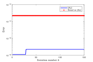
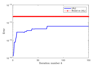
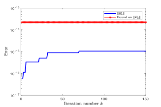
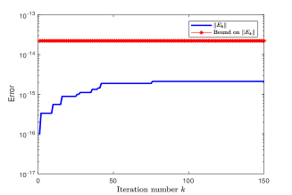
It is remarkable to notice that (40) holds without depending on the orthogonality levels of Uk+1,Vksubscript𝑈𝑘1subscript𝑉𝑘U_{k+1},\ V_{k} and V~ksubscript~𝑉𝑘\widetilde{V}_{k}. Since (40) indicates that the squares of singular values of Bksubscript𝐵𝑘B_{k} and B¯ksubscript¯𝐵𝑘\bar{B}_{k} can be determined each other with the error O(ϵ)𝑂italic-ϵO(\epsilon), it can be used to design algorithms for the GSVD computation. Therefore, if some extreme generalized singular values of {A,L}𝐴𝐿\{A,L\} are desired, then, except the approach that computes the generalized singular values of {Bk,B¯k}subscript𝐵𝑘subscript¯𝐵𝑘\{B_{k},\bar{B}_{k}\} and uses extreme ones to approximate the corresponding ones of {A,L}𝐴𝐿\{A,L\}, an alternative is to compute the singular values of Bksubscript𝐵𝑘B_{k} or B^ksubscript^𝐵𝑘\widehat{B}_{k} (or equivalently B¯ksubscript¯𝐵𝑘\bar{B}_{k}) to obtain approximate generalized singular values. For a convergence analysis of the singular values of Bksubscript𝐵𝑘B_{k} to some of QAsubscript𝑄𝐴Q_{A} and more details, we refer the reader to [10, 11]. We will propose the JBD method for the GSVD computation and consider some details in Section 4, where we will revisit (40).

Since Bksubscript𝐵𝑘B_{k} and B¯ksubscript¯𝐵𝑘\bar{B}_{k} have full column rank, by (40) we have

(BkT)(BkTBk+B¯kTB¯k)B¯k1superscriptsuperscriptsubscript𝐵𝑘𝑇superscriptsubscript𝐵𝑘𝑇subscript𝐵𝑘superscriptsubscript¯𝐵𝑘𝑇subscript¯𝐵𝑘superscriptsubscript¯𝐵𝑘1\displaystyle(B_{k}^{T})^{{\dagger}}(B_{k}^{T}B_{k}+\bar{B}_{k}^{T}\bar{B}_{k})\bar{B}_{k}^{-1} =(BkT)B¯k1+(BkT)EkB¯k1absentsuperscriptsuperscriptsubscript𝐵𝑘𝑇superscriptsubscript¯𝐵𝑘1superscriptsuperscriptsubscript𝐵𝑘𝑇subscript𝐸𝑘superscriptsubscript¯𝐵𝑘1\displaystyle=(B_{k}^{T})^{{\dagger}}\bar{B}_{k}^{-1}+(B_{k}^{T})^{{\dagger}}E_{k}\bar{B}_{k}^{-1}
=(B¯kBkT)+(BkT)EkB¯k1,absentsuperscriptsubscript¯𝐵𝑘superscriptsubscript𝐵𝑘𝑇superscriptsuperscriptsubscript𝐵𝑘𝑇subscript𝐸𝑘superscriptsubscript¯𝐵𝑘1\displaystyle=(\bar{B}_{k}B_{k}^{T})^{{\dagger}}+(B_{k}^{T})^{{\dagger}}E_{k}\bar{B}_{k}^{-1},

which leads to

(B¯kBkT)=(BkT)BkTBkB¯k1+(BkT)B¯kT(BkT)EkB¯k1.superscriptsubscript¯𝐵𝑘superscriptsubscript𝐵𝑘𝑇superscriptsuperscriptsubscript𝐵𝑘𝑇superscriptsubscript𝐵𝑘𝑇subscript𝐵𝑘superscriptsubscript¯𝐵𝑘1superscriptsuperscriptsubscript𝐵𝑘𝑇superscriptsubscript¯𝐵𝑘𝑇superscriptsuperscriptsubscript𝐵𝑘𝑇subscript𝐸𝑘superscriptsubscript¯𝐵𝑘1(\bar{B}_{k}B_{k}^{T})^{{\dagger}}=(B_{k}^{T})^{{\dagger}}B_{k}^{T}B_{k}\bar{B}_{k}^{-1}+(B_{k}^{T})^{{\dagger}}\bar{B}_{k}^{T}-(B_{k}^{T})^{{\dagger}}E_{k}\bar{B}_{k}^{-1}.

Since BkT=(B¯k,βk+1ek)superscriptsubscript𝐵𝑘𝑇matrixsubscript¯𝐵𝑘subscript𝛽𝑘1subscript𝑒𝑘B_{k}^{T}=\begin{pmatrix}\underline{B}_{k},\beta_{k+1}e_{k}\end{pmatrix}, we have (BkT)B¯k1normsuperscriptsuperscriptsubscript𝐵𝑘𝑇normsuperscriptsubscript¯𝐵𝑘1\|(B_{k}^{T})^{{\dagger}}\|\leq\|\underline{B}_{k}^{-1}\|. Notice that (BkT)BkT=1normsuperscriptsuperscriptsubscript𝐵𝑘𝑇superscriptsubscript𝐵𝑘𝑇1\|(B_{k}^{T})^{{\dagger}}B_{k}^{T}\|=1. From (38) and (39), we obtain

(B¯kBkT)2(B¯k1+B¯k1)+c0(ϵ),normsuperscriptsubscript¯𝐵𝑘superscriptsubscript𝐵𝑘𝑇2normsuperscriptsubscript¯𝐵𝑘1normsuperscriptsubscript¯𝐵𝑘1subscript𝑐0italic-ϵ\|(\bar{B}_{k}B_{k}^{T})^{{\dagger}}\|\leq\sqrt{2}(\|\bar{B}_{k}^{-1}\|+\|\underline{B}_{k}^{-1}\|)+c_{0}(\epsilon),

where

c0(ϵ)=B¯k1B¯k1O(c3(m,n,p)ϵ).subscript𝑐0italic-ϵnormsuperscriptsubscript¯𝐵𝑘1normsuperscriptsubscript¯𝐵𝑘1𝑂subscript𝑐3𝑚𝑛𝑝italic-ϵc_{0}(\epsilon)=\|\bar{B}_{k}^{-1}\|\|\underline{B}_{k}^{-1}\|O(c_{3}(m,n,p)\epsilon).

Since B¯kBkT=(B¯kB¯k,βk+1B¯kek)subscript¯𝐵𝑘superscriptsubscript𝐵𝑘𝑇matrixsubscript¯𝐵𝑘subscript¯𝐵𝑘subscript𝛽𝑘1subscript¯𝐵𝑘subscript𝑒𝑘\bar{B}_{k}B_{k}^{T}=\begin{pmatrix}\bar{B}_{k}\underline{B}_{k},\beta_{k+1}\bar{B}_{k}e_{k}\end{pmatrix}, by the interlacing property of singular values, we have σk(B¯kB¯k)σk(B¯kBkT)subscript𝜎𝑘subscript¯𝐵𝑘subscript¯𝐵𝑘subscript𝜎𝑘subscript¯𝐵𝑘superscriptsubscript𝐵𝑘𝑇\sigma_{k}(\bar{B}_{k}\underline{B}_{k})\leq\sigma_{k}(\bar{B}_{k}B_{k}^{T}), where σi()subscript𝜎𝑖\sigma_{i}(\cdot) denotes the i𝑖i-th largest singular value of a matrix, proving that (B¯kBkT)(B¯kB¯k)1normsuperscriptsubscript¯𝐵𝑘superscriptsubscript𝐵𝑘𝑇normsuperscriptsubscript¯𝐵𝑘subscript¯𝐵𝑘1\|(\bar{B}_{k}B_{k}^{T})^{{\dagger}}\|\leq\|(\bar{B}_{k}\underline{B}_{k})^{-1}\|. However, in our experiments, it has been found that (B¯kB¯k)1c¯(B¯kBkT)normsuperscriptsubscript¯𝐵𝑘subscript¯𝐵𝑘1¯𝑐normsuperscriptsubscript¯𝐵𝑘superscriptsubscript𝐵𝑘𝑇\|(\bar{B}_{k}\underline{B}_{k})^{-1}\|\leq\bar{c}\|(\bar{B}_{k}B_{k}^{T})^{{\dagger}}\| always holds with a modest constant c¯=O(1)¯𝑐𝑂1\bar{c}=O(1), usually c¯5¯𝑐5\bar{c}\leq 5. Notice that c0(ϵ)subscript𝑐0italic-ϵc_{0}(\epsilon) is much smaller than B¯k1+B¯k1normsuperscriptsubscript¯𝐵𝑘1normsuperscriptsubscript¯𝐵𝑘1\|\bar{B}_{k}^{-1}\|+\|\underline{B}_{k}^{-1}\|. Therefore, in the sequel we will suppose and use the following upper bound for (B¯kB¯k)1normsuperscriptsubscript¯𝐵𝑘subscript¯𝐵𝑘1\|(\bar{B}_{k}\underline{B}_{k})^{-1}\|:

(43) (B¯kB¯k)1c2(B¯k1+B¯k1),normsuperscriptsubscript¯𝐵𝑘subscript¯𝐵𝑘1𝑐2normsuperscriptsubscript¯𝐵𝑘1normsuperscriptsubscript¯𝐵𝑘1\|(\bar{B}_{k}\underline{B}_{k})^{-1}\|\leq c\sqrt{2}(\|\bar{B}_{k}^{-1}\|+\|\underline{B}_{k}^{-1}\|),

where c>1𝑐1c>1 slightly.

We next establish a relationship between the JBD process for computing B^ksubscript^𝐵𝑘\widehat{B}_{k} and the upper Lanczos bidiagonalization of QLsubscript𝑄𝐿Q_{L} in finite precision.

Theorem 3.

With the hypothesis of Theorem 1, in finite precision, we have

(44) QLV^ksubscript𝑄𝐿subscript^𝑉𝑘\displaystyle Q_{L}\widehat{V}_{k} =\displaystyle= U^kB^k+F^k,subscript^𝑈𝑘subscript^𝐵𝑘subscript^𝐹𝑘\displaystyle\widehat{U}_{k}\widehat{B}_{k}+\widehat{F}_{k},
(45) QLTU^ksuperscriptsubscript𝑄𝐿𝑇subscript^𝑈𝑘\displaystyle Q_{L}^{T}\widehat{U}_{k} =\displaystyle= V^kB^kT+β^kv^k+1ekT+G^ksubscript^𝑉𝑘superscriptsubscript^𝐵𝑘𝑇subscript^𝛽𝑘subscript^𝑣𝑘1superscriptsubscript𝑒𝑘𝑇subscript^𝐺𝑘\displaystyle\widehat{V}_{k}\widehat{B}_{k}^{T}+\hat{\beta}_{k}\hat{v}_{k+1}e_{k}^{T}+\widehat{G}_{k}

with

(46) F^knormsubscript^𝐹𝑘\displaystyle\|\widehat{F}_{k}\| =\displaystyle= O(B¯k1ϵ),\displaystyle O(\lVert\underline{B}_{k}^{-1}\lVert\epsilon),
(47) G^knormsubscript^𝐺𝑘\displaystyle\|\widehat{G}_{k}\| =\displaystyle= O(c4(m,n,p,k)ϵ)𝑂subscript𝑐4𝑚𝑛𝑝𝑘italic-ϵ\displaystyle O(c_{4}(m,n,p,k)\epsilon)

with

(48) c4(m,n,p,k)=B¯k1+c3(m,n,p)B^k1.subscript𝑐4𝑚𝑛𝑝𝑘normsuperscriptsubscript¯𝐵𝑘1subscript𝑐3𝑚𝑛𝑝normsuperscriptsubscript^𝐵𝑘1c_{4}(m,n,p,k)=\|\underline{B}_{k}^{-1}\|+c_{3}(m,n,p)\|\widehat{B}_{k}^{-1}\|.
Proof.

Recall the notation in (5), (15) and (10). Then exploiting Lemma 3.1, we can rewrite (23) as

(0p×m,Ip)V^k=U^kB^k+F^k,subscript0𝑝𝑚subscript𝐼𝑝subscript^𝑉𝑘subscript^𝑈𝑘subscript^𝐵𝑘subscript^𝐹𝑘(0_{p\times m},I_{p})\widehat{V}_{k}=\widehat{U}_{k}\widehat{B}_{k}+\widehat{F}_{k},

where

(49) F^k=F¯k(0p×m,Ip)(V~kQVk)Dk.subscript^𝐹𝑘subscript¯𝐹𝑘subscript0𝑝𝑚subscript𝐼𝑝subscript~𝑉𝑘𝑄subscript𝑉𝑘subscript𝐷𝑘\widehat{F}_{k}=\bar{F}_{k}-(0_{p\times m},I_{p})(\widetilde{V}_{k}-QV_{k})D_{k}.

Therefore, (44) holds.

From (32) and (33), we obtain

(50) QATQAVk=QATUk+1Bk+QATFk=(VkBkT+αk+1vk+1ek+1T+Gk+1)Bk+QATFk=VkBkTBk+αk+1βk+1vk+1ekT+Gk+1Bk+QATFk.superscriptsubscript𝑄𝐴𝑇subscript𝑄𝐴subscript𝑉𝑘superscriptsubscript𝑄𝐴𝑇subscript𝑈𝑘1subscript𝐵𝑘superscriptsubscript𝑄𝐴𝑇subscript𝐹𝑘subscript𝑉𝑘superscriptsubscript𝐵𝑘𝑇subscript𝛼𝑘1subscript𝑣𝑘1superscriptsubscript𝑒𝑘1𝑇subscript𝐺𝑘1subscript𝐵𝑘superscriptsubscript𝑄𝐴𝑇subscript𝐹𝑘subscript𝑉𝑘superscriptsubscript𝐵𝑘𝑇subscript𝐵𝑘subscript𝛼𝑘1subscript𝛽𝑘1subscript𝑣𝑘1superscriptsubscript𝑒𝑘𝑇subscript𝐺𝑘1subscript𝐵𝑘superscriptsubscript𝑄𝐴𝑇subscript𝐹𝑘\displaystyle\begin{split}Q_{A}^{T}Q_{A}V_{k}&=Q_{A}^{T}U_{k+1}B_{k}+Q_{A}^{T}F_{k}\\ &=(V_{k}B_{k}^{T}+\alpha_{k+1}v_{k+1}e_{k+1}^{T}+G_{k+1})B_{k}+Q_{A}^{T}F_{k}\\ &=V_{k}B_{k}^{T}B_{k}+\alpha_{k+1}\beta_{k+1}v_{k+1}e_{k}^{T}+G_{k+1}B_{k}+Q_{A}^{T}F_{k}.\end{split}

Premultiplying and postmultiplying (44) by QLTsuperscriptsubscript𝑄𝐿𝑇Q_{L}^{T} and Dksubscript𝐷𝑘D_{k} gives

QLTQLVk=(QLTU^kB^k+QLTF^k)Dk.superscriptsubscript𝑄𝐿𝑇subscript𝑄𝐿subscript𝑉𝑘superscriptsubscript𝑄𝐿𝑇subscript^𝑈𝑘subscript^𝐵𝑘superscriptsubscript𝑄𝐿𝑇subscript^𝐹𝑘subscript𝐷𝑘Q_{L}^{T}Q_{L}V_{k}=(Q_{L}^{T}\widehat{U}_{k}\widehat{B}_{k}+Q_{L}^{T}\widehat{F}_{k})D_{k}.

Summing the above two equalities yields

Vksubscript𝑉𝑘\displaystyle V_{k} =(QATQA+QLTQL)Vkabsentsuperscriptsubscript𝑄𝐴𝑇subscript𝑄𝐴superscriptsubscript𝑄𝐿𝑇subscript𝑄𝐿subscript𝑉𝑘\displaystyle=(Q_{A}^{T}Q_{A}+Q_{L}^{T}Q_{L})V_{k}
=VkBkTBk+QLTU^kB^kDk+αk+1βk+1vk+1ekT+(Gk+1Bk+QATFk+QLTF^kDk)absentsubscript𝑉𝑘superscriptsubscript𝐵𝑘𝑇subscript𝐵𝑘superscriptsubscript𝑄𝐿𝑇subscript^𝑈𝑘subscript^𝐵𝑘subscript𝐷𝑘subscript𝛼𝑘1subscript𝛽𝑘1subscript𝑣𝑘1superscriptsubscript𝑒𝑘𝑇subscript𝐺𝑘1subscript𝐵𝑘superscriptsubscript𝑄𝐴𝑇subscript𝐹𝑘superscriptsubscript𝑄𝐿𝑇subscript^𝐹𝑘subscript𝐷𝑘\displaystyle=V_{k}B_{k}^{T}B_{k}+Q_{L}^{T}\widehat{U}_{k}\widehat{B}_{k}D_{k}+\alpha_{k+1}\beta_{k+1}v_{k+1}e_{k}^{T}+(G_{k+1}B_{k}+Q_{A}^{T}F_{k}+Q_{L}^{T}\widehat{F}_{k}D_{k})
=Vk(IkDkB^kTB^kDk+Ek)+QLTU^kB^kDk+αk+1βk+1vk+1ekTabsentsubscript𝑉𝑘subscript𝐼𝑘subscript𝐷𝑘superscriptsubscript^𝐵𝑘𝑇subscript^𝐵𝑘subscript𝐷𝑘subscript𝐸𝑘superscriptsubscript𝑄𝐿𝑇subscript^𝑈𝑘subscript^𝐵𝑘subscript𝐷𝑘subscript𝛼𝑘1subscript𝛽𝑘1subscript𝑣𝑘1superscriptsubscript𝑒𝑘𝑇\displaystyle=V_{k}(I_{k}-D_{k}\widehat{B}_{k}^{T}\widehat{B}_{k}D_{k}+E_{k})+Q_{L}^{T}\widehat{U}_{k}\widehat{B}_{k}D_{k}+\alpha_{k+1}\beta_{k+1}v_{k+1}e_{k}^{T}
+(Gk+1Bk+QATFk+QLTF^kDk).subscript𝐺𝑘1subscript𝐵𝑘superscriptsubscript𝑄𝐴𝑇subscript𝐹𝑘superscriptsubscript𝑄𝐿𝑇subscript^𝐹𝑘subscript𝐷𝑘\displaystyle\ \ \ \ +(G_{k+1}B_{k}+Q_{A}^{T}F_{k}+Q_{L}^{T}\widehat{F}_{k}D_{k}).

From this relation, V^k=VkDksubscript^𝑉𝑘subscript𝑉𝑘subscript𝐷𝑘\widehat{V}_{k}=V_{k}D_{k} and Dk2=Iksuperscriptsubscript𝐷𝑘2subscript𝐼𝑘D_{k}^{2}=I_{k} it follows that

V^kB^kTB^ksubscript^𝑉𝑘superscriptsubscript^𝐵𝑘𝑇subscript^𝐵𝑘\displaystyle\widehat{V}_{k}\widehat{B}_{k}^{T}\widehat{B}_{k} =QLTU^kB^k+αk+1βk+1vk+1ekTDk+(Gk+1Bk+QATFk+QLTF^kDk+VkEk)Dkabsentsuperscriptsubscript𝑄𝐿𝑇subscript^𝑈𝑘subscript^𝐵𝑘subscript𝛼𝑘1subscript𝛽𝑘1subscript𝑣𝑘1superscriptsubscript𝑒𝑘𝑇subscript𝐷𝑘subscript𝐺𝑘1subscript𝐵𝑘superscriptsubscript𝑄𝐴𝑇subscript𝐹𝑘superscriptsubscript𝑄𝐿𝑇subscript^𝐹𝑘subscript𝐷𝑘subscript𝑉𝑘subscript𝐸𝑘subscript𝐷𝑘\displaystyle=Q_{L}^{T}\widehat{U}_{k}\widehat{B}_{k}+\alpha_{k+1}\beta_{k+1}v_{k+1}e_{k}^{T}D_{k}+(G_{k+1}B_{k}+Q_{A}^{T}F_{k}+Q_{L}^{T}\widehat{F}_{k}D_{k}+V_{k}E_{k})D_{k}
=QLTU^kB^k(α^kβ^k+γk)v^k+1ekT+(Gk+1Bk+QATFk+QLTF^kDk+VkEk)Dk,absentsuperscriptsubscript𝑄𝐿𝑇subscript^𝑈𝑘subscript^𝐵𝑘subscript^𝛼𝑘subscript^𝛽𝑘subscript𝛾𝑘subscript^𝑣𝑘1superscriptsubscript𝑒𝑘𝑇subscript𝐺𝑘1subscript𝐵𝑘superscriptsubscript𝑄𝐴𝑇subscript𝐹𝑘superscriptsubscript𝑄𝐿𝑇subscript^𝐹𝑘subscript𝐷𝑘subscript𝑉𝑘subscript𝐸𝑘subscript𝐷𝑘\displaystyle=Q_{L}^{T}\widehat{U}_{k}\widehat{B}_{k}-(\hat{\alpha}_{k}\hat{\beta}_{k}+\gamma_{k})\hat{v}_{k+1}e_{k}^{T}+(G_{k+1}B_{k}+Q_{A}^{T}F_{k}+Q_{L}^{T}\widehat{F}_{k}D_{k}+V_{k}E_{k})D_{k},

which shows that

V^kB^kT=QLTU^kβ^kv^k+1ekT+E1+E2,subscript^𝑉𝑘superscriptsubscript^𝐵𝑘𝑇superscriptsubscript𝑄𝐿𝑇subscript^𝑈𝑘subscript^𝛽𝑘subscript^𝑣𝑘1superscriptsubscript𝑒𝑘𝑇subscript𝐸1subscript𝐸2\widehat{V}_{k}\widehat{B}_{k}^{T}=Q_{L}^{T}\widehat{U}_{k}-\hat{\beta}_{k}\hat{v}_{k+1}e_{k}^{T}+E_{1}+E_{2},

where

E1=[(Gk+1Bk+VkEk)Dkγkv^k+1ekT]B^k1,E2=(QATFkDk+QLTF^k)B^k1.formulae-sequencesubscript𝐸1delimited-[]subscript𝐺𝑘1subscript𝐵𝑘subscript𝑉𝑘subscript𝐸𝑘subscript𝐷𝑘subscript𝛾𝑘subscript^𝑣𝑘1superscriptsubscript𝑒𝑘𝑇superscriptsubscript^𝐵𝑘1subscript𝐸2superscriptsubscript𝑄𝐴𝑇subscript𝐹𝑘subscript𝐷𝑘superscriptsubscript𝑄𝐿𝑇subscript^𝐹𝑘superscriptsubscript^𝐵𝑘1E_{1}=[(G_{k+1}B_{k}+V_{k}E_{k})D_{k}-\gamma_{k}\hat{v}_{k+1}e_{k}^{T}]\widehat{B}_{k}^{-1},\ \ E_{2}=(Q_{A}^{T}F_{k}D_{k}+Q_{L}^{T}\widehat{F}_{k})\widehat{B}_{k}^{-1}.

From (20), we have Vk1+η(Vk)normsubscript𝑉𝑘1𝜂subscript𝑉𝑘\|V_{k}\|\leq\sqrt{1+\eta(V_{k})}. Notice that γksubscript𝛾𝑘\gamma_{k} in (41) satisfies |γk|=O(ϵ)subscript𝛾𝑘𝑂italic-ϵ|\gamma_{k}|=O(\epsilon) and the elements of Eknormsubscript𝐸𝑘\|E_{k}\| in (40) are O(c3(m,n,p))𝑂subscript𝑐3𝑚𝑛𝑝O(c_{3}(m,n,p)). Using the upper bounds for Bknormsubscript𝐵𝑘\|B_{k}\| in (38), we have

E1=O(c¯1(m,n,p,k)ϵ)normsubscript𝐸1𝑂subscript¯𝑐1𝑚𝑛𝑝𝑘italic-ϵ\|E_{1}\|=O(\bar{c}_{1}(m,n,p,k)\epsilon)

with c¯1(m,n,p,k)=(2+c3(m,n,p))B^k1subscript¯𝑐1𝑚𝑛𝑝𝑘2subscript𝑐3𝑚𝑛𝑝normsuperscriptsubscript^𝐵𝑘1\bar{c}_{1}(m,n,p,k)=(\sqrt{2}+c_{3}(m,n,p))\|\widehat{B}_{k}^{-1}\|. Using the expressions of Fksubscript𝐹𝑘F_{k}, F^ksubscript^𝐹𝑘\widehat{F}_{k} and V~kQVksubscript~𝑉𝑘𝑄subscript𝑉𝑘\widetilde{V}_{k}-QV_{k} in (31), (49) and (29), respectively, we have

QATFkDk+QLTF^ksuperscriptsubscript𝑄𝐴𝑇subscript𝐹𝑘subscript𝐷𝑘superscriptsubscript𝑄𝐿𝑇subscript^𝐹𝑘\displaystyle Q_{A}^{T}F_{k}D_{k}+Q_{L}^{T}\widehat{F}_{k} =(QATQLT)(FkDkF^k)absentmatrixsuperscriptsubscript𝑄𝐴𝑇superscriptsubscript𝑄𝐿𝑇matrixsubscript𝐹𝑘subscript𝐷𝑘subscript^𝐹𝑘\displaystyle=\begin{pmatrix}Q_{A}^{T}&Q_{L}^{T}\end{pmatrix}\begin{pmatrix}F_{k}D_{k}\\ \widehat{F}_{k}\end{pmatrix}
=QT[(F~kDkF¯k)(Im0m×p0p×mIp)(V~kQVk)Dk]absentsuperscript𝑄𝑇delimited-[]matrixsubscript~𝐹𝑘subscript𝐷𝑘subscript¯𝐹𝑘matrixsubscript𝐼𝑚subscript0𝑚𝑝subscript0𝑝𝑚subscript𝐼𝑝subscript~𝑉𝑘𝑄subscript𝑉𝑘subscript𝐷𝑘\displaystyle=Q^{T}\Big{[}\begin{pmatrix}\widetilde{F}_{k}D_{k}\\ \bar{F}_{k}\end{pmatrix}-\begin{pmatrix}I_{m}&0_{m\times p}\\ 0_{p\times m}&I_{p}\end{pmatrix}(\widetilde{V}_{k}-QV_{k})D_{k}\Big{]}
=QT[(F~kDkF¯k)+(Im+pQQT)G~kB¯k1Dk].absentsuperscript𝑄𝑇delimited-[]matrixsubscript~𝐹𝑘subscript𝐷𝑘subscript¯𝐹𝑘subscript𝐼𝑚𝑝𝑄superscript𝑄𝑇subscript~𝐺𝑘superscriptsubscript¯𝐵𝑘1subscript𝐷𝑘\displaystyle=Q^{T}\Big{[}\begin{pmatrix}\widetilde{F}_{k}D_{k}\\ \bar{F}_{k}\end{pmatrix}+(I_{m+p}-QQ^{T})\widetilde{G}_{k}\underline{B}_{k}^{-1}D_{k}\Big{]}.

From (43), we obtain

B¯k1DkB^k1=(B¯kB¯k)1c2(B¯k1+B¯k1).normsuperscriptsubscript¯𝐵𝑘1subscript𝐷𝑘superscriptsubscript^𝐵𝑘1normsuperscriptsubscript¯𝐵𝑘subscript¯𝐵𝑘1𝑐2normsuperscriptsubscript¯𝐵𝑘1normsuperscriptsubscript¯𝐵𝑘1\|\underline{B}_{k}^{-1}D_{k}\widehat{B}_{k}^{-1}\|=\|(\bar{B}_{k}\underline{B}_{k})^{-1}\|\leq c\sqrt{2}(\|\bar{B}_{k}^{-1}\|+\|\underline{B}_{k}^{-1}\|).

Since B¯k1=B^k1normsuperscriptsubscript¯𝐵𝑘1normsuperscriptsubscript^𝐵𝑘1\|\bar{B}_{k}^{-1}\|=\|\widehat{B}_{k}^{-1}\|, it holds that

E2=O(c¯2(k)ϵ)normsubscript𝐸2𝑂subscript¯𝑐2𝑘italic-ϵ\|E_{2}\|=O(\bar{c}_{2}(k)\epsilon)

with c¯2(k)=c2(B^k1+B¯k1)+B^k1subscript¯𝑐2𝑘𝑐2normsuperscriptsubscript^𝐵𝑘1normsuperscriptsubscript¯𝐵𝑘1normsuperscriptsubscript^𝐵𝑘1\bar{c}_{2}(k)=c\sqrt{2}(\|\widehat{B}_{k}^{-1}\|+\|\underline{B}_{k}^{-1}\|)+\|\widehat{B}_{k}^{-1}\|. Letting G^k=E1E2subscript^𝐺𝑘subscript𝐸1subscript𝐸2\widehat{G}_{k}=-E_{1}-E_{2} leads to the desired result. ∎

Notice that (44) and (45) are the corresponding versions of (10) in the presence of rounding errors. Therefore, this theorem indicates that the JBD process for computing U^ksubscript^𝑈𝑘\widehat{U}_{k}, V^ksubscript^𝑉𝑘\widehat{V}_{k} and B^ksubscript^𝐵𝑘\widehat{B}_{k} is no longer equivalent to the standard upper Lanczos bidiagonalization of QLsubscript𝑄𝐿Q_{L} with the rounding error O(QLϵ)=O(ϵ)𝑂normsubscript𝑄𝐿italic-ϵ𝑂italic-ϵO(\|Q_{L}\|\epsilon)=O(\epsilon) in finite precision, since the error terms F^ksubscript^𝐹𝑘\widehat{F}_{k} and G^ksubscript^𝐺𝑘\widehat{G}_{k} are amplified gradually once B¯k1normsuperscriptsubscript¯𝐵𝑘1\|\underline{B}_{k}^{-1}\| and B^k1normsuperscriptsubscript^𝐵𝑘1\|\widehat{B}_{k}^{-1}\| grow as k𝑘k increases.

In summary, unlike standard lower and upper Lanczos bidiagonalizations of QAsubscript𝑄𝐴Q_{A} and QLsubscript𝑄𝐿Q_{L} in finite precision, the JBD process in finite precision is lower and upper Lanczos bidiagonalizations with gradually growing error terms, where the growths of the error terms are dictated by B¯k1normsuperscriptsubscript¯𝐵𝑘1\|\underline{B}_{k}^{-1}\| and B^k1normsuperscriptsubscript^𝐵𝑘1\|\widehat{B}_{k}^{-1}\| separately.

3.2 Loss of orthogonality of the Lanczos vectors

It is well known that, for Lanczos bidiagonalization, the numerical orthogonality of Lanczos vectors is gradually lost due to the influence of rounding errors. Once the orthogonality is lost at one iteration, the errors will propagate to later steps, which leads to the more loss of orthogonality of subsequently computed Lanczos vectors [18, 30]. For the JBD process, there is similar loss of orthogonality of each of the three sets of basis vectors. As it will turn out, the orthogonality levels of Uk+1subscript𝑈𝑘1U_{k+1}, V~ksubscript~𝑉𝑘\widetilde{V}_{k} and U^ksubscript^𝑈𝑘\widehat{U}_{k} are closely related and interact. Below we prove how the orthogonality level of U^ksubscript^𝑈𝑘\widehat{U}_{k} is affected by those of both Uk+1subscript𝑈𝑘1U_{k+1} and V~ksubscript~𝑉𝑘\widetilde{V}_{k}.

Theorem 4.

With the hypothesis of Theorem 1, in finite precision, we have

(51) η(U^k)B^k12[η(V~k)+2η(Uk+1)+O(c3(m,n,p)ϵ)].𝜂subscript^𝑈𝑘superscriptnormsuperscriptsubscript^𝐵𝑘12delimited-[]𝜂subscript~𝑉𝑘2𝜂subscript𝑈𝑘1𝑂subscript𝑐3𝑚𝑛𝑝italic-ϵ\eta(\widehat{U}_{k})\leq\|\widehat{B}_{k}^{-1}\|^{2}\big{[}\eta(\widetilde{V}_{k})+2\eta(U_{k+1})+O(c_{3}(m,n,p)\epsilon)\big{]}.
Proof.

From (21) and (23), we have

V~k=(Uk+1BkU^kB¯k)+(F~kF¯kDk),subscript~𝑉𝑘matrixsubscript𝑈𝑘1subscript𝐵𝑘subscript^𝑈𝑘subscript¯𝐵𝑘matrixsubscript~𝐹𝑘subscript¯𝐹𝑘subscript𝐷𝑘\widetilde{V}_{k}=\begin{pmatrix}U_{k+1}B_{k}\\ \widehat{U}_{k}\bar{B}_{k}\end{pmatrix}+\begin{pmatrix}\widetilde{F}_{k}\\ \bar{F}_{k}D_{k}\end{pmatrix},

which shows that

(52) V~kTV~k=BkTUk+1TUk+1Bk+B¯kTU^kTU^kB¯k+E3,superscriptsubscript~𝑉𝑘𝑇subscript~𝑉𝑘superscriptsubscript𝐵𝑘𝑇superscriptsubscript𝑈𝑘1𝑇subscript𝑈𝑘1subscript𝐵𝑘superscriptsubscript¯𝐵𝑘𝑇superscriptsubscript^𝑈𝑘𝑇subscript^𝑈𝑘subscript¯𝐵𝑘subscript𝐸3\widetilde{V}_{k}^{T}\widetilde{V}_{k}=B_{k}^{T}U_{k+1}^{T}U_{k+1}B_{k}+\bar{B}_{k}^{T}\widehat{U}_{k}^{T}\widehat{U}_{k}\bar{B}_{k}+E_{3},

where

E3=BkTUk+1TF~k+B¯kTU^kTF¯kP+F~kTUk+1Bk+PF¯kTU^kB¯k+F~kTF~k+PF¯kTF¯kDk.subscript𝐸3superscriptsubscript𝐵𝑘𝑇superscriptsubscript𝑈𝑘1𝑇subscript~𝐹𝑘superscriptsubscript¯𝐵𝑘𝑇superscriptsubscript^𝑈𝑘𝑇subscript¯𝐹𝑘𝑃superscriptsubscript~𝐹𝑘𝑇subscript𝑈𝑘1subscript𝐵𝑘𝑃superscriptsubscript¯𝐹𝑘𝑇subscript^𝑈𝑘subscript¯𝐵𝑘superscriptsubscript~𝐹𝑘𝑇subscript~𝐹𝑘𝑃superscriptsubscript¯𝐹𝑘𝑇subscript¯𝐹𝑘subscript𝐷𝑘E_{3}=B_{k}^{T}U_{k+1}^{T}\widetilde{F}_{k}+\bar{B}_{k}^{T}\widehat{U}_{k}^{T}\bar{F}_{k}P+\widetilde{F}_{k}^{T}U_{k+1}B_{k}+P\bar{F}_{k}^{T}\widehat{U}_{k}\bar{B}_{k}+\widetilde{F}_{k}^{T}\widetilde{F}_{k}+P\bar{F}_{k}^{T}\bar{F}_{k}D_{k}.

From (40), we obtain

IkV~kTV~k=BkT(Ik+1Uk+1TUk+1)Bk+B¯kT(IkU^kTU^k)B¯kEkE3,subscript𝐼𝑘superscriptsubscript~𝑉𝑘𝑇subscript~𝑉𝑘superscriptsubscript𝐵𝑘𝑇subscript𝐼𝑘1superscriptsubscript𝑈𝑘1𝑇subscript𝑈𝑘1subscript𝐵𝑘superscriptsubscript¯𝐵𝑘𝑇subscript𝐼𝑘superscriptsubscript^𝑈𝑘𝑇subscript^𝑈𝑘subscript¯𝐵𝑘subscript𝐸𝑘subscript𝐸3I_{k}-\widetilde{V}_{k}^{T}\widetilde{V}_{k}=B_{k}^{T}(I_{k+1}-U_{k+1}^{T}U_{k+1})B_{k}+\bar{B}_{k}^{T}(I_{k}-\widehat{U}_{k}^{T}\widehat{U}_{k})\bar{B}_{k}-E_{k}-E_{3},

which, together with (52), yields

(53) IkU^kTU^k=B¯kT[(IkV~kTV~k)BkT(Ik+1Uk+1TUk+1)Bk+Ek+E3]B¯k1.subscript𝐼𝑘superscriptsubscript^𝑈𝑘𝑇subscript^𝑈𝑘superscriptsubscript¯𝐵𝑘𝑇delimited-[]subscript𝐼𝑘superscriptsubscript~𝑉𝑘𝑇subscript~𝑉𝑘superscriptsubscript𝐵𝑘𝑇subscript𝐼𝑘1superscriptsubscript𝑈𝑘1𝑇subscript𝑈𝑘1subscript𝐵𝑘subscript𝐸𝑘subscript𝐸3superscriptsubscript¯𝐵𝑘1I_{k}-\widehat{U}_{k}^{T}\widehat{U}_{k}=\bar{B}_{k}^{-T}\big{[}(I_{k}-\widetilde{V}_{k}^{T}\widetilde{V}_{k})-B_{k}^{T}(I_{k+1}-U_{k+1}^{T}U_{k+1})B_{k}+E_{k}+E_{3}\big{]}\bar{B}_{k}^{-1}.

Notice that Uk+1(1+η(Uk+1))1/2normsubscript𝑈𝑘1superscript1𝜂subscript𝑈𝑘112\|U_{k+1}\|\leq(1+\eta(U_{k+1}))^{1/2} and U^k(1+η(U^k))1/2normsubscript^𝑈𝑘superscript1𝜂subscript^𝑈𝑘12\|\widehat{U}_{k}\|\leq(1+\eta(\widehat{U}_{k}))^{1/2}. Using the bounds for Bknormsubscript𝐵𝑘\|B_{k}\| and B^knormsubscript^𝐵𝑘\|\widehat{B}_{k}\| in (38) and (39), respectively, by a simple calculation, we obtain

E3=O(ϵ).normsubscript𝐸3𝑂italic-ϵ\|E_{3}\|=O(\epsilon).

Using the bound for Bknormsubscript𝐵𝑘\|B_{k}\|, we have

BkT(Ik+1Uk+1TUk+1)Bknormsuperscriptsubscript𝐵𝑘𝑇subscript𝐼𝑘1superscriptsubscript𝑈𝑘1𝑇subscript𝑈𝑘1subscript𝐵𝑘\displaystyle\|B_{k}^{T}(I_{k+1}-U_{k+1}^{T}U_{k+1})B_{k}\| Bk2Ik+1Uk+1TUk+1absentsuperscriptnormsubscript𝐵𝑘2normsubscript𝐼𝑘1superscriptsubscript𝑈𝑘1𝑇subscript𝑈𝑘1\displaystyle\leq\|B_{k}\|^{2}\|I_{k+1}-U_{k+1}^{T}U_{k+1}\|
2Ik+1Uk+1TUk+1+O(c1(m,n)ϵ).absent2normsubscript𝐼𝑘1superscriptsubscript𝑈𝑘1𝑇subscript𝑈𝑘1𝑂subscript𝑐1𝑚𝑛italic-ϵ\displaystyle\leq 2\|I_{k+1}-U_{k+1}^{T}U_{k+1}\|+O(c_{1}(m,n)\epsilon).

Taking norms in (53) proves the desired result. ∎

The above theorem indicates that as long as B^ksubscript^𝐵𝑘\widehat{B}_{k} is not ill conditioned, the orthogonality of U^ksubscript^𝑈𝑘\widehat{U}_{k} is as good as those of Uk+1subscript𝑈𝑘1U_{k+1} and V~ksubscript~𝑉𝑘\widetilde{V}_{k}. Therefore, it is only necessary to perform some sort of reorthogonalization strategies to maintain desired orthogonality levels of Uk+1subscript𝑈𝑘1U_{k+1} and V~ksubscript~𝑉𝑘\widetilde{V}_{k}.

The following result shows that the orthogonality levels of the long V~k(m+p)×ksubscript~𝑉𝑘superscript𝑚𝑝𝑘\widetilde{V}_{k}\in\mathbb{R}^{(m+p)\times k} and the short Vkp×ksubscript𝑉𝑘superscript𝑝𝑘V_{k}\in\mathbb{R}^{p\times k} are the same within O(ϵ)𝑂italic-ϵO(\epsilon) under some mild condition.

Theorem 5.

With definition (19), it holds that

(54) |η(V~k)η(Vk)|=O(B¯k12ϵ2).|\eta(\widetilde{V}_{k})-\eta(V_{k})|=O(\lVert\underline{B}_{k}^{-1}\lVert^{2}\epsilon^{2}).
Proof.

From (29), we have

V~kT(Im+pQQT)V~ksuperscriptsubscript~𝑉𝑘𝑇subscript𝐼𝑚𝑝𝑄superscript𝑄𝑇subscript~𝑉𝑘\displaystyle\widetilde{V}_{k}^{T}(I_{m+p}-QQ^{T})\widetilde{V}_{k} =V~kT(V~kQVk)=V~kT(QQTIm+p)G~kB¯k1absentsuperscriptsubscript~𝑉𝑘𝑇subscript~𝑉𝑘𝑄subscript𝑉𝑘superscriptsubscript~𝑉𝑘𝑇𝑄superscript𝑄𝑇subscript𝐼𝑚𝑝subscript~𝐺𝑘superscriptsubscript¯𝐵𝑘1\displaystyle=\widetilde{V}_{k}^{T}(\widetilde{V}_{k}-QV_{k})=\widetilde{V}_{k}^{T}(QQ^{T}-I_{m+p})\widetilde{G}_{k}\underline{B}_{k}^{-1}
=[(Im+pQQT)V~k]TG~kB¯k1absentsuperscriptdelimited-[]subscript𝐼𝑚𝑝𝑄superscript𝑄𝑇subscript~𝑉𝑘𝑇subscript~𝐺𝑘superscriptsubscript¯𝐵𝑘1\displaystyle=-[(I_{m+p}-QQ^{T})\widetilde{V}_{k}]^{T}\widetilde{G}_{k}\underline{B}_{k}^{-1}
=B¯kTG~kT(Im+pQQT)G~kB¯k1.absentsuperscriptsubscript¯𝐵𝑘𝑇superscriptsubscript~𝐺𝑘𝑇subscript𝐼𝑚𝑝𝑄superscript𝑄𝑇subscript~𝐺𝑘superscriptsubscript¯𝐵𝑘1\displaystyle=\underline{B}_{k}^{-T}\widetilde{G}_{k}^{T}(I_{m+p}-QQ^{T})\widetilde{G}_{k}\underline{B}_{k}^{-1}.

Thus

IkVkTVk=IkV~kTQQTV~k=IkV~kTV~k+V~kT(Im+pQQT)V~k=(IkV~kTV~k)+B¯kTG~kT(Im+pQQT)G~kB¯k1.subscript𝐼𝑘superscriptsubscript𝑉𝑘𝑇subscript𝑉𝑘subscript𝐼𝑘superscriptsubscript~𝑉𝑘𝑇𝑄superscript𝑄𝑇subscript~𝑉𝑘subscript𝐼𝑘superscriptsubscript~𝑉𝑘𝑇subscript~𝑉𝑘superscriptsubscript~𝑉𝑘𝑇subscript𝐼𝑚𝑝𝑄superscript𝑄𝑇subscript~𝑉𝑘subscript𝐼𝑘superscriptsubscript~𝑉𝑘𝑇subscript~𝑉𝑘superscriptsubscript¯𝐵𝑘𝑇superscriptsubscript~𝐺𝑘𝑇subscript𝐼𝑚𝑝𝑄superscript𝑄𝑇subscript~𝐺𝑘superscriptsubscript¯𝐵𝑘1\displaystyle\begin{split}I_{k}-V_{k}^{T}V_{k}&=I_{k}-\widetilde{V}_{k}^{T}QQ^{T}\widetilde{V}_{k}=I_{k}-\widetilde{V}_{k}^{T}\widetilde{V}_{k}+\widetilde{V}_{k}^{T}(I_{m+p}-QQ^{T})\widetilde{V}_{k}\\ &=(I_{k}-\widetilde{V}_{k}^{T}\widetilde{V}_{k})+\underline{B}_{k}^{-T}\widetilde{G}_{k}^{T}(I_{m+p}-QQ^{T})\widetilde{G}_{k}\underline{B}_{k}^{-1}.\end{split}

Therefore, (54) holds. ∎

This theorem shows that provided that B¯k1normsuperscriptsubscript¯𝐵𝑘1\|\underline{B}_{k}^{-1}\| is not too big, say no more than ϵ1/2superscriptitalic-ϵ12\epsilon^{-1/2}, we have |η(V~k)η(Vk)|=O(ϵ)𝜂subscript~𝑉𝑘𝜂subscript𝑉𝑘𝑂italic-ϵ|\eta(\widetilde{V}_{k})-\eta(V_{k})|=O(\epsilon). Therefore, it is only necessary to maintain the same orthogonality level of Vksubscript𝑉𝑘V_{k} in order to make V~ksubscript~𝑉𝑘\widetilde{V}_{k} achieve a desired orthogonality level. From (51), this shows that we only need to maintain desired orthogonality levels of Uk+1subscript𝑈𝑘1U_{k+1} and Vksubscript𝑉𝑘V_{k} so as to make U^ksubscript^𝑈𝑘\widehat{U}_{k} have a desired orthogonality level.

4 The JBD method for the GSVD computation

In this section, we review how to use the JBD process to compute some extreme GSVD components of {A,L}𝐴𝐿\{A,L\} [37], which leads to the JBD method for the large GSVD computation, and make an analysis on the convergence of the approximate generalized singular values in finite precision by exploiting the previous results.

4.1 The JBD method

For ease of presentation, we do not take into account rounding errors when computing the GSVD of {Bk,B¯k}subscript𝐵𝑘subscript¯𝐵𝑘\{B_{k},\bar{B}_{k}\} or the SVD of Bksubscript𝐵𝑘B_{k} or B^ksubscript^𝐵𝑘\widehat{B}_{k}, that is, we assume that the compact SVD of Bksubscript𝐵𝑘B_{k} is computed accurately:

(55) Bk=PkΘkWkT,Θk=diag(c1(k),,ck(k)), 1c1(k)>>ck(k)0,formulae-sequencesubscript𝐵𝑘subscript𝑃𝑘subscriptΘ𝑘superscriptsubscript𝑊𝑘𝑇formulae-sequencesubscriptΘ𝑘diagsuperscriptsubscript𝑐1𝑘superscriptsubscript𝑐𝑘𝑘1superscriptsubscript𝑐1𝑘superscriptsubscript𝑐𝑘𝑘0B_{k}=P_{k}\Theta_{k}W_{k}^{T},\ \ \Theta_{k}=\mathop{\operator@font diag}\nolimits(c_{1}^{(k)},\dots,c_{k}^{(k)}),\ \ 1\geq c_{1}^{(k)}>\dots>c_{k}^{(k)}\geq 0,

where Pk=(p1(k),,pk(k))(k+1)×ksubscript𝑃𝑘superscriptsubscript𝑝1𝑘superscriptsubscript𝑝𝑘𝑘superscript𝑘1𝑘P_{k}=(p_{1}^{(k)},\dots,p_{k}^{(k)})\in\mathbb{R}^{(k+1)\times k} is orthonormal and Wk=(w1(k),,wk(k))k×ksubscript𝑊𝑘superscriptsubscript𝑤1𝑘superscriptsubscript𝑤𝑘𝑘superscript𝑘𝑘W_{k}=(w_{1}^{(k)},\dots,w_{k}^{(k)})\in\mathbb{R}^{k\times k} is orthogonal. The SVD (55) can be obtained by a standard SVD algorithm since Bksubscript𝐵𝑘B_{k} is small sized. Then we have k𝑘k approximate generalized singular values {ci(k),(1(ci(k))2)1/2}superscriptsubscript𝑐𝑖𝑘superscript1superscriptsuperscriptsubscript𝑐𝑖𝑘212\{c_{i}^{(k)},(1-(c_{i}^{(k)})^{2})^{1/2}\}, i=1,2,,k𝑖12𝑘i=1,2,\ldots,k of {A,L}𝐴𝐿\{A,L\}, and the approximate right generalized singular vectors are the xi(k)=R1Vkwi(k)superscriptsubscript𝑥𝑖𝑘superscript𝑅1subscript𝑉𝑘superscriptsubscript𝑤𝑖𝑘x_{i}^{(k)}=R^{-1}V_{k}w_{i}^{(k)} and the approximations to the left generalized singular vectors piAsuperscriptsubscript𝑝𝑖𝐴p_{i}^{A} are yi(k)=Uk+1pi(k)superscriptsubscript𝑦𝑖𝑘subscript𝑈𝑘1superscriptsubscript𝑝𝑖𝑘y_{i}^{(k)}=U_{k+1}p_{i}^{(k)}. Among these k𝑘k approximations, we pick up a few largest and/or smallest ones as approximations to the largest and/or smallest ci/sisubscript𝑐𝑖subscript𝑠𝑖c_{i}/s_{i} and the corresponding xisubscript𝑥𝑖x_{i} and piAsuperscriptsubscript𝑝𝑖𝐴p_{i}^{A}.

If we also want to compute an approximation of the left generalized singular vector piLsuperscriptsubscript𝑝𝑖𝐿p_{i}^{L}, we need to compute the SVD of B¯ksubscript¯𝐵𝑘\bar{B}_{k}. From (17), it is known that (BkT,B¯kT)Tsuperscriptsuperscriptsubscript𝐵𝑘𝑇superscriptsubscript¯𝐵𝑘𝑇𝑇(B_{k}^{T},\bar{B}_{k}^{T})^{T} is column orthonormal. Therefore, the CS decomposition of the pair {Bk,B¯k}subscript𝐵𝑘subscript¯𝐵𝑘\{B_{k},\bar{B}_{k}\} is its GSVD, and that the right singular vectors of Bksubscript𝐵𝑘B_{k} and B¯ksubscript¯𝐵𝑘\bar{B}_{k} are identical. As a result, we can assume that the SVD of B¯ksubscript¯𝐵𝑘\bar{B}_{k} is

(56) B¯k=P¯kΨkWkT,Ψk=diag(s¯1(k),,s¯k(k)), 0s¯1(k)<<s¯k(k)1,formulae-sequencesubscript¯𝐵𝑘subscript¯𝑃𝑘subscriptΨ𝑘superscriptsubscript𝑊𝑘𝑇formulae-sequencesubscriptΨ𝑘diagsuperscriptsubscript¯𝑠1𝑘superscriptsubscript¯𝑠𝑘𝑘 0superscriptsubscript¯𝑠1𝑘superscriptsubscript¯𝑠𝑘𝑘1\bar{B}_{k}=\bar{P}_{k}\Psi_{k}W_{k}^{T},\ \ \Psi_{k}={\rm diag}(\bar{s}_{1}^{(k)},\dots,\bar{s}_{k}^{(k)}),\ \ 0\leq\bar{s}_{1}^{(k)}<\dots<\bar{s}_{k}^{(k)}\leq 1\ ,

where P¯k=(p¯1(k),,p¯k(k))k×ksubscript¯𝑃𝑘superscriptsubscript¯𝑝1𝑘superscriptsubscript¯𝑝𝑘𝑘superscript𝑘𝑘\bar{P}_{k}=(\bar{p}_{1}^{(k)},\dots,\bar{p}_{k}^{(k)})\in\mathbb{R}^{k\times k} and Wk=(w1(k),,wk(k))k×ksubscript𝑊𝑘superscriptsubscript𝑤1𝑘superscriptsubscript𝑤𝑘𝑘superscript𝑘𝑘W_{k}=(w_{1}^{(k)},\dots,w_{k}^{(k)})\in\mathbb{R}^{k\times k} are orthogonal. Then zi(k)=U^kp¯i(k)superscriptsubscript𝑧𝑖𝑘subscript^𝑈𝑘superscriptsubscript¯𝑝𝑖𝑘z_{i}^{(k)}=\widehat{U}_{k}\bar{p}_{i}^{(k)} is an approximation to piLsuperscriptsubscript𝑝𝑖𝐿p_{i}^{L}. The approximate generalized singular values and the corresponding approximate right generalized singular vectors are {(1(s¯i(k))2)1/2,s¯i(k)}superscript1superscriptsuperscriptsubscript¯𝑠𝑖𝑘212superscriptsubscript¯𝑠𝑖𝑘\{(1-(\bar{s}_{i}^{(k)})^{2})^{1/2},\bar{s}_{i}^{(k)}\} and R1Vkwi(k)superscript𝑅1subscript𝑉𝑘superscriptsubscript𝑤𝑖𝑘R^{-1}V_{k}w_{i}^{(k)}, respectively. We have seen that the approximate right generalized singular vectors obtained by the SVDs of Bksubscript𝐵𝑘B_{k} and B¯ksubscript¯𝐵𝑘\bar{B}_{k} are the same, as expected. We also comment that if the JBD process is performed in exact arithmetic then mathematically s¯i(k)=si(k)=1(ci(k))2superscriptsubscript¯𝑠𝑖𝑘superscriptsubscript𝑠𝑖𝑘1superscriptsuperscriptsubscript𝑐𝑖𝑘2\bar{s}_{i}^{(k)}=s_{i}^{(k)}=\sqrt{1-(c_{i}^{(k)})^{2}}.

Alternatively, we compute the GSVD of the pair {Bk,B¯k}subscript𝐵𝑘subscript¯𝐵𝑘\{B_{k},\bar{B}_{k}\}:

(57) Bk=PkCkWkT,B¯k=P¯kSkWkT,formulae-sequencesubscript𝐵𝑘subscript𝑃𝑘subscript𝐶𝑘superscriptsubscript𝑊𝑘𝑇subscript¯𝐵𝑘subscript¯𝑃𝑘subscript𝑆𝑘superscriptsubscript𝑊𝑘𝑇B_{k}=P_{k}C_{k}W_{k}^{T},\ \bar{B}_{k}=\bar{P}_{k}S_{k}W_{k}^{T},

where Ck=diag(c1(k),,ck(k))subscript𝐶𝑘diagsuperscriptsubscript𝑐1𝑘superscriptsubscript𝑐𝑘𝑘C_{k}={\rm diag}(c_{1}^{(k)},\ldots,c_{k}^{(k)}) and Sk=diag(s1(k),,sk(k))subscript𝑆𝑘diagsuperscriptsubscript𝑠1𝑘superscriptsubscript𝑠𝑘𝑘S_{k}={\rm diag}(s_{1}^{(k)},\ldots,s_{k}^{(k)}), and Pksubscript𝑃𝑘P_{k} and P¯ksubscript¯𝑃𝑘\bar{P}_{k} are as those defined in (55) and (56). The approximate generalized singular values are {ci(k),si(k)}superscriptsubscript𝑐𝑖𝑘superscriptsubscript𝑠𝑖𝑘\{c_{i}^{(k)},s_{i}^{(k)}\} or ci(k)/si(k)superscriptsubscript𝑐𝑖𝑘superscriptsubscript𝑠𝑖𝑘c_{i}^{(k)}/s_{i}^{(k)}, the corresponding left approximate generalized singular vectors for A𝐴A and L𝐿L are Uk+1pi(k)subscript𝑈𝑘1superscriptsubscript𝑝𝑖𝑘U_{k+1}p_{i}^{(k)} and U^kp¯i(k)subscript^𝑈𝑘superscriptsubscript¯𝑝𝑖𝑘\widehat{U}_{k}\bar{p}_{i}^{(k)}, respectively, and the right approximate generalized singular vectors are xi(k)=Zkwi(k)=R1Vkwi(k)superscriptsubscript𝑥𝑖𝑘subscript𝑍𝑘superscriptsubscript𝑤𝑖𝑘superscript𝑅1subscript𝑉𝑘superscriptsubscript𝑤𝑖𝑘x_{i}^{(k)}=Z_{k}w_{i}^{(k)}=R^{-1}V_{k}w_{i}^{(k)}.

We remark that, in finite precision, the ci(k)superscriptsubscript𝑐𝑖𝑘c_{i}^{(k)} and si(k)superscriptsubscript𝑠𝑖𝑘s_{i}^{(k)} in the GSVD of {Bk,B¯k}subscript𝐵𝑘subscript¯𝐵𝑘\{B_{k},\bar{B}_{k}\} are computed with no loss of accuracy and satisfy (ci(k))2+(si(k))2=1superscriptsuperscriptsubscript𝑐𝑖𝑘2superscriptsuperscriptsubscript𝑠𝑖𝑘21(c_{i}^{(k)})^{2}+(s_{i}^{(k)})^{2}=1 unconditionally within working precision, irrespective of their sizes. In contrast, it is easily justified from (40) that if either of Bksubscript𝐵𝑘B_{k} and B¯ksubscript¯𝐵𝑘\bar{B}_{k} is ill conditioned then (1(ci(k))2)1/2superscript1superscriptsuperscriptsubscript𝑐𝑖𝑘212(1-(c_{i}^{(k)})^{2})^{1/2} or (1(s¯i(k))2)1/2superscript1superscriptsuperscriptsubscript¯𝑠𝑖𝑘212(1-(\bar{s}_{i}^{(k)})^{2})^{1/2} as the singular values of B¯ksubscript¯𝐵𝑘\bar{B}_{k} or Bksubscript𝐵𝑘B_{k} may be inaccurate when (ci(k))2=1O(ϵ)superscriptsuperscriptsubscript𝑐𝑖𝑘21𝑂italic-ϵ(c_{i}^{(k)})^{2}=1-O(\epsilon) or (s¯i(k))2=1O(ϵ)superscriptsuperscriptsubscript¯𝑠𝑖𝑘21𝑂italic-ϵ(\bar{s}_{i}^{(k)})^{2}=1-O(\epsilon), which corresponds to an ill-conditioned B¯ksubscript¯𝐵𝑘\bar{B}_{k} or Bksubscript𝐵𝑘B_{k} with small singular values no more than O(ϵ1/2)𝑂superscriptitalic-ϵ12O(\epsilon^{1/2}), respectively. In other words, if B¯ksubscript¯𝐵𝑘\bar{B}_{k} is ill conditioned and has a singular value no more than O(ϵ1/2)𝑂superscriptitalic-ϵ12O(\epsilon^{1/2}), one would compute it with no accuracy from the corresponding singular value of Bksubscript𝐵𝑘B_{k}, and vice versa. In this case, the corresponding approximate generalized singular values may be quite inaccurate and even has no accuracy; for the accuracy and reliability, we suggest to compute the singular values ci(k)superscriptsubscript𝑐𝑖𝑘c_{i}^{(k)} and s¯i(k)superscriptsubscript¯𝑠𝑖𝑘\bar{s}_{i}^{(k)} of both Bksubscript𝐵𝑘B_{k} and B¯ksubscript¯𝐵𝑘\bar{B}_{k} separately and use {ci(k),s¯i(k)}superscriptsubscript𝑐𝑖𝑘superscriptsubscript¯𝑠𝑖𝑘\{c_{i}^{(k)},\bar{s}_{i}^{(k)}\} as approximations to some extreme {ci,si}subscript𝑐𝑖subscript𝑠𝑖\{c_{i},s_{i}\}.

For the computation of xi(k)superscriptsubscript𝑥𝑖𝑘x_{i}^{(k)}, it is shown in [37] that the explicit inversion R1superscript𝑅1R^{-1} can be avoided by noticing that

(58) (AL)xi(k)=QRR1Vkwi(k)=V~kwi(k).matrix𝐴𝐿superscriptsubscript𝑥𝑖𝑘𝑄𝑅superscript𝑅1subscript𝑉𝑘superscriptsubscript𝑤𝑖𝑘subscript~𝑉𝑘superscriptsubscript𝑤𝑖𝑘\begin{pmatrix}A\\ L\end{pmatrix}x_{i}^{(k)}=QRR^{-1}V_{k}w_{i}^{(k)}=\widetilde{V}_{k}w_{i}^{(k)}.

Then, solving the corresponding consistent linear system by an iterative solver, e.g., the LSQR algorithm, we obtain xi(k)superscriptsubscript𝑥𝑖𝑘x_{i}^{(k)}.

4.2 Convergence, accuracy and reorthogonalization

In the presence of rounding errors, the behavior of the JBD algorithm may deviate from that in exact arithmetic. As mentioned previously, we only consider the rounding errors in the JBD process, and assume that the SVDs of Bksubscript𝐵𝑘B_{k} and B¯ksubscript¯𝐵𝑘\bar{B}_{k} are computed accurately, so are xi(k)superscriptsubscript𝑥𝑖𝑘x_{i}^{(k)}, yi(k)superscriptsubscript𝑦𝑖𝑘y_{i}^{(k)} and zi(k)superscriptsubscript𝑧𝑖𝑘z_{i}^{(k)}.

First, we investigate the convergence of the computed generalized singular values using the SVD of Bksubscript𝐵𝑘B_{k}. Since ci2+si2=1superscriptsubscript𝑐𝑖2superscriptsubscript𝑠𝑖21c_{i}^{2}+s_{i}^{2}=1, in order to compute the generalized singular value {ci,si}subscript𝑐𝑖subscript𝑠𝑖\{c_{i},s_{i}\}, we only need to compute cisubscript𝑐𝑖c_{i}, which is a singular value of QAsubscript𝑄𝐴Q_{A}. Note that ci(k)superscriptsubscript𝑐𝑖𝑘c_{i}^{(k)}, the singular value of Bksubscript𝐵𝑘B_{k}, is a computed Ritz value of QAsubscript𝑄𝐴Q_{A}, due to the property that the k𝑘k-step JBD process for computing Bksubscript𝐵𝑘B_{k} is Lanczos bidiagonalization applied to QAsubscript𝑄𝐴Q_{A} with the rounding error O(B¯k1ϵ)O(\lVert\underline{B}_{k}^{-1}\lVert\epsilon); see Theorem 1. In exact arithmetic, it is shown in [15] that the eigenvalues of BkTBksuperscriptsubscript𝐵𝑘𝑇subscript𝐵𝑘B_{k}^{T}B_{k} are the Ritz values of QATQAsuperscriptsubscript𝑄𝐴𝑇subscript𝑄𝐴Q_{A}^{T}Q_{A} with respect to the Krylov subspace generated by QATb,(QATQA)QATb,,(QATQA)k1QATbsuperscriptsubscript𝑄𝐴𝑇𝑏superscriptsubscript𝑄𝐴𝑇subscript𝑄𝐴superscriptsubscript𝑄𝐴𝑇𝑏superscriptsuperscriptsubscript𝑄𝐴𝑇subscript𝑄𝐴𝑘1superscriptsubscript𝑄𝐴𝑇𝑏Q_{A}^{T}b,(Q_{A}^{T}Q_{A})Q_{A}^{T}b,\ldots,(Q_{A}^{T}Q_{A})^{k-1}Q_{A}^{T}b and the k𝑘k-step lower bidiagonalization of QAsubscript𝑄𝐴Q_{A} is equivalent to the symmetric Lanczos process applied to QATQAsuperscriptsubscript𝑄𝐴𝑇subscript𝑄𝐴Q_{A}^{T}Q_{A} and the starting vector QATb/QATbsuperscriptsubscript𝑄𝐴𝑇𝑏normsuperscriptsubscript𝑄𝐴𝑇𝑏Q_{A}^{T}b/\|Q_{A}^{T}b\| that generates the symmetric tridiagonal matrix BkTBksuperscriptsubscript𝐵𝑘𝑇subscript𝐵𝑘B_{k}^{T}B_{k} and an orthonormal basis matrix Vksubscript𝑉𝑘V_{k} of the aforementioned Krylov subspace. Therefore, the convergence theory of the symmetric Lanczos method applies (cf. [27, 29]), and the singular values of Bksubscript𝐵𝑘B_{k} generally favor some largest and smallest ones of QAsubscript𝑄𝐴Q_{A}. More convergence results and details have been given in [9, 10, 15]. In finite precision, typical convergence features of the symmetric Lanczos method carry over to our case, which include: (a) the computed Ritz values generally favor the extreme singular values of QAsubscript𝑄𝐴Q_{A}, while interior singular values are hard to be approximated; (b) if the extreme singular values of QAsubscript𝑄𝐴Q_{A} are better separated one another, the corresponding computed Ritz values converge more rapidly. As a result, if we compute cisubscript𝑐𝑖c_{i} by the SVD of Bksubscript𝐵𝑘B_{k}, the computed Ritz values approximating the extreme generalized singular values of {A,L}𝐴𝐿\{A,L\} will first converge generally.

In finite precision, some of the singular values of Bksubscript𝐵𝑘B_{k} could be numerically multiple as the iteration number k𝑘k increases, which may produce ghost approximations to some generalized singular values of {A,L}𝐴𝐿\{A,L\}. A direct consequence is that a simple or genuine multiple generalized singular value of {A,L}𝐴𝐿\{A,L\} could be approximated by numerically multiple computed Ritz values, which could lead to a convergence delay of computed Ritz values. This phenomenon could occur only when the computed Lanczos vectors lose orthogonality and can be avoided by using some types of reorthogonalization strategies, such as full reorthogonalization or the more efficient one-sided reorthogonalization [32].

By Theorem 1, the JBD process for computing Bksubscript𝐵𝑘B_{k} is the lower Lanczos bidiagonalization of QAsubscript𝑄𝐴Q_{A} with the rounding error O(B¯k1ϵ)𝑂normsuperscriptsubscript¯𝐵𝑘1italic-ϵO(\|\underline{B}_{k}^{-1}\|\epsilon) that is comparable to O(ϵ)𝑂italic-ϵO(\epsilon) whenever B¯k1normsuperscriptsubscript¯𝐵𝑘1\|\underline{B}_{k}^{-1}\| is modest. If the JBD process is implemented with one-sided reorthogonalization of visubscript𝑣𝑖v_{i} such that the orthogonality level of Vksubscript𝑉𝑘V_{k} achieves O(ϵ)𝑂italic-ϵO(\epsilon), exploiting the backward error results on the Lanczos bidiagonalization with one-sided reorthogonalization [1, Theorem 5.2 and Corollary 5.1], we can deduce that the computed Bksubscript𝐵𝑘B_{k} is the exact one generated by the Lanczos bidiagonalization of a nearby matrix QA+Eksubscript𝑄𝐴subscript𝐸𝑘Q_{A}+E_{k} with Ek=O(B¯k1ϵ)normsubscript𝐸𝑘𝑂normsuperscriptsubscript¯𝐵𝑘1italic-ϵ\|E_{k}\|=O(\|\underline{B}_{k}^{-1}\|\epsilon). Therefore, by the perturbation theory of the singular values [5, Corollary 8.6.2], the extreme singular values of QAsubscript𝑄𝐴Q_{A} can be computed with the ultimate accuracy O(B¯k1ϵ)𝑂normsuperscriptsubscript¯𝐵𝑘1italic-ϵO(\|\underline{B}_{k}^{-1}\|\epsilon), and ghost Ritz values can be avoided.

It is known that a necessary orthogonality level of the computed basis vectors is the semiorthogonality for the symmetric Lanczos process [27, 30] and Lanczos bidiagonalization [18]. Based on Theorem 1 and [18, Theorem 5], it is straightforward to prove that the semiorthogonality suffices in finite precision.

Theorem 6.

Assume that the compact QR factorizations of Uk+1subscript𝑈𝑘1U_{k+1} and Vksubscript𝑉𝑘V_{k} are Uk+1=Mk+1Rk+1subscript𝑈𝑘1subscript𝑀𝑘1subscript𝑅𝑘1U_{k+1}=M_{k+1}R_{k+1} and Vk=NkSksubscript𝑉𝑘subscript𝑁𝑘subscript𝑆𝑘V_{k}=N_{k}S_{k}, where the diagonals of Rk+1subscript𝑅𝑘1R_{k+1} and Sksubscript𝑆𝑘S_{k} are positive, and let δ=O(B¯k1ϵ)𝛿𝑂normsuperscriptsubscript¯𝐵𝑘1italic-ϵ\delta=O(\|\underline{B}_{k}^{-1}\|\epsilon). If Uk+1subscript𝑈𝑘1U_{k+1} and Vksubscript𝑉𝑘V_{k} satisfy the semiorthogonality

(59) ξ(Uk+1),ξ(Vk)δ/(2k+1),𝜉subscript𝑈𝑘1𝜉subscript𝑉𝑘𝛿2𝑘1\xi(U_{k+1}),\ \xi(V_{k})\leqslant\sqrt{\delta/(2k+1)},

then

(60) Mk+1TQANk=Bk+E~k,superscriptsubscript𝑀𝑘1𝑇subscript𝑄𝐴subscript𝑁𝑘subscript𝐵𝑘subscript~𝐸𝑘M_{k+1}^{T}Q_{A}N_{k}=B_{k}+\widetilde{E}_{k},

where the elements of E~ksubscript~𝐸𝑘\widetilde{E}_{k} are O(δ)=O(B¯k1ϵ)𝑂𝛿𝑂normsuperscriptsubscript¯𝐵𝑘1italic-ϵO(\delta)=O(\|\underline{B}_{k}^{-1}\|\epsilon) in size.

Notice that Mk+1TQANksuperscriptsubscript𝑀𝑘1𝑇subscript𝑄𝐴subscript𝑁𝑘M_{k+1}^{T}Q_{A}N_{k} is precisely the Ritz–Galerkin projection matrix of QAsubscript𝑄𝐴Q_{A} with respect to the left and right subspaces span(Uk+1)spansubscript𝑈𝑘1{\rm span}(U_{k+1}) and span(Vk)spansubscript𝑉𝑘{\rm span}(V_{k}), whose singular values are the true Ritz values of QAsubscript𝑄𝐴Q_{A} with respect to these two subspaces in exact arithmetic, while the singular values of Bksubscript𝐵𝑘B_{k} are the computed Ritz values only when semiorthogonality is met. Theorem 6 indicates that once the orthogonality levels of Uk+1subscript𝑈𝑘1U_{k+1} and Vksubscript𝑉𝑘V_{k} are below (δ/(2k+1))1/2superscript𝛿2𝑘112(\delta/(2k+1))^{1/2}, the computed Ritz values are close to those true ones within O(ϵ)𝑂italic-ϵO(\epsilon) provided that B¯k1normsuperscriptsubscript¯𝐵𝑘1\|\underline{B}_{k}^{-1}\| is modest. Since the true Ritz values are never ghosts provided that no breakdown occurs before iteration k𝑘k, we avoid the appearance of ghost computed Ritz values whenever Uk+1subscript𝑈𝑘1U_{k+1} and Vksubscript𝑉𝑘V_{k} have semiorthogonality. Consequently, as long as true Ritz values are approximations to some singular values of QAsubscript𝑄𝐴Q_{A} with the accuracy O(B¯k1ϵ)𝑂normsuperscriptsubscript¯𝐵𝑘1italic-ϵO(\|\underline{B}_{k}^{-1}\|\epsilon), the corresponding computed Ritz values have the same approximation accuracy too. In the meantime, it is easily justified that, when Uk+1subscript𝑈𝑘1U_{k+1} and Vksubscript𝑉𝑘V_{k} have full orthogonality levels O(ϵ)𝑂italic-ϵO(\epsilon), Theorem 6 holds with the norm of the error matrix in the right-hand side still being O(B¯k1ϵ)𝑂normsuperscriptsubscript¯𝐵𝑘1italic-ϵO(\|\underline{B}_{k}^{-1}\|\epsilon). Therefore, the semiorthogonality of Uk+1subscript𝑈𝑘1U_{k+1} and Vksubscript𝑉𝑘V_{k} suffices for computing generalized singular values accurately. We have made a detailed investigation on the JBD process with semiorthogonalization strategy and proposed an efficient partial reorthogonalization strategy in [12].

There is a corresponding counterpart of Theorem 6 for B¯ksubscript¯𝐵𝑘\bar{B}_{k}, as stated blow.

Theorem 7.

Let δ^=O(c4(m,n,p,k)ϵ)^𝛿𝑂subscript𝑐4𝑚𝑛𝑝𝑘italic-ϵ\hat{\delta}=O(c_{4}(m,n,p,k)\epsilon) with c4(m,n,p,k)subscript𝑐4𝑚𝑛𝑝𝑘c_{4}(m,n,p,k) defined by (48), and the compact QR factorizations of U^ksubscript^𝑈𝑘\widehat{U}_{k} and Vksubscript𝑉𝑘V_{k} be U^k=M^kR^ksubscript^𝑈𝑘subscript^𝑀𝑘subscript^𝑅𝑘\widehat{U}_{k}=\widehat{M}_{k}\widehat{R}_{k} and Vk=NkSksubscript𝑉𝑘subscript𝑁𝑘subscript𝑆𝑘V_{k}=N_{k}S_{k}, where the diagonals of R^ksubscript^𝑅𝑘\widehat{R}_{k} and Sksubscript𝑆𝑘S_{k} are positive. If U^ksubscript^𝑈𝑘\widehat{U}_{k} and V^ksubscript^𝑉𝑘\widehat{V}_{k} satisfy the semiorthogonality

ξ(U^k),ξ(Vk)δ^/(2k+1),𝜉subscript^𝑈𝑘𝜉subscript𝑉𝑘^𝛿2𝑘1\xi(\widehat{U}_{k}),\ \xi(V_{k})\leqslant\sqrt{\hat{\delta}/(2k+1)},

then

M^kTQLNk=B¯k+E¯k,superscriptsubscript^𝑀𝑘𝑇subscript𝑄𝐿subscript𝑁𝑘subscript¯𝐵𝑘subscript¯𝐸𝑘\widehat{M}_{k}^{T}Q_{L}N_{k}=\bar{B}_{k}+\bar{E}_{k},

where the elements of E¯ksubscript¯𝐸𝑘\bar{E}_{k} are O(δ^)=O((B¯k1+B¯k1)ϵ)𝑂^𝛿𝑂normsuperscriptsubscript¯𝐵𝑘1normsuperscriptsubscript¯𝐵𝑘1italic-ϵO(\hat{\delta})=O((\|\underline{B}_{k}^{-1}\|+\|\bar{B}_{k}^{-1}\|)\epsilon) in size.

Comparing Theorem 7 with Theorem 6, we find that Theorem 7 requires that B¯k1normsuperscriptsubscript¯𝐵𝑘1\|\underline{B}_{k}^{-1}\| and B¯k1normsuperscriptsubscript¯𝐵𝑘1\|\bar{B}_{k}^{-1}\| be controllable, stronger than the requirement of Theorem 6.

4.3 Residual norm and stopping criterion

Now we concentrate on designing an effective and efficient stopping criterion for the GSVD computation based on the JBD process. Still, we only assume rounding errors in the JBD process, and suppose that the other computations are exact. The following analysis focuses on computing some extreme GSVD components of {A,L}𝐴𝐿\{A,L\} using the SVD of Bksubscript𝐵𝑘B_{k}.

From the GSVD (7) of {A,L}𝐴𝐿\{A,L\}, it is known that the generalized eigenvalues λ𝜆\lambda of the symmetric generalized eigenvalue problem ATAx=λLTLxsuperscript𝐴𝑇𝐴𝑥𝜆superscript𝐿𝑇𝐿𝑥A^{T}Ax=\lambda L^{T}Lx are

,,q,(cq+1/sq+1)2,,(cq+l/sq+l)2l,0,,0t,subscript𝑞subscriptsuperscriptsubscript𝑐𝑞1subscript𝑠𝑞12superscriptsubscript𝑐𝑞𝑙subscript𝑠𝑞𝑙2𝑙subscript00𝑡\underbrace{\infty,\dots,\infty}_{q},\ \ \underbrace{(c_{q+1}/s_{q+1})^{2},\dots,(c_{q+l}/s_{q+l})^{2}}_{l},\ \ \underbrace{0,\dots,0}_{t},

and the corresponding generalized eigenvectors x𝑥x are the right generalized singular vectors x𝑥x of {A,L}𝐴𝐿\{A,L\}. The generalized eigenvalue problem ATAxi=λiLTLxisuperscript𝐴𝑇𝐴subscript𝑥𝑖subscript𝜆𝑖superscript𝐿𝑇𝐿subscript𝑥𝑖A^{T}Ax_{i}=\lambda_{i}L^{T}Lx_{i} can be equivalently written as si2ATAxi=ci2LTLxisuperscriptsubscript𝑠𝑖2superscript𝐴𝑇𝐴subscript𝑥𝑖superscriptsubscript𝑐𝑖2superscript𝐿𝑇𝐿subscript𝑥𝑖s_{i}^{2}A^{T}Ax_{i}=c_{i}^{2}L^{T}Lx_{i}. Based on this equivalence, Zha in [37] uses the residual norm

(61) ri(k)=((si(k))2ATA(ci(k))2LTL)xi(k)normsuperscriptsubscript𝑟𝑖𝑘normsuperscriptsuperscriptsubscript𝑠𝑖𝑘2superscript𝐴𝑇𝐴superscriptsuperscriptsubscript𝑐𝑖𝑘2superscript𝐿𝑇𝐿superscriptsubscript𝑥𝑖𝑘\|r_{i}^{(k)}\|=\|((s_{i}^{(k)})^{2}A^{T}A-(c_{i}^{(k)})^{2}L^{T}L)x_{i}^{(k)}\|

to design a stopping criterion for an approximate generalized singular value pair {ci(k),si(k)}superscriptsubscript𝑐𝑖𝑘superscriptsubscript𝑠𝑖𝑘\{c_{i}^{(k)},s_{i}^{(k)}\} and the corresponding right vector xi(k)superscriptsubscript𝑥𝑖𝑘x_{i}^{(k)}, where (ci(k))2+(si(k))2=1superscriptsuperscriptsubscript𝑐𝑖𝑘2superscriptsuperscriptsubscript𝑠𝑖𝑘21(c_{i}^{(k)})^{2}+(s_{i}^{(k)})^{2}=1. Clearly, the computation of ri(k)normsuperscriptsubscript𝑟𝑖𝑘\|r_{i}^{(k)}\| is expensive since it needs to compute xi(k)superscriptsubscript𝑥𝑖𝑘x_{i}^{(k)} explicitly by solving a large scale least squares problem like (58) at each iteration k𝑘k until the convergence occurs, where wi(k)superscriptsubscript𝑤𝑖𝑘w_{i}^{(k)} depends on the approach used in the JBD method; see Section 4.1. In exact arithmetic, Zha [37] has proved a sharp bound:

(62) ri(k)Rαk+1βk+1|ekTwi(k)|normsuperscriptsubscript𝑟𝑖𝑘norm𝑅subscript𝛼𝑘1subscript𝛽𝑘1superscriptsubscript𝑒𝑘𝑇superscriptsubscript𝑤𝑖𝑘\|r_{i}^{(k)}\|\leq\|R\|\alpha_{k+1}\beta_{k+1}|e_{k}^{T}w_{i}^{(k)}|

with R𝑅R defined in (1), so that Rαk+1βk+1|ekTwi(k)|norm𝑅subscript𝛼𝑘1subscript𝛽𝑘1superscriptsubscript𝑒𝑘𝑇superscriptsubscript𝑤𝑖𝑘\|R\|\alpha_{k+1}\beta_{k+1}|e_{k}^{T}w_{i}^{(k)}| can be used to design a stopping criterion if Rnorm𝑅\|R\| or its reasonable estimate is available. From (1), for C=(AT,LT)T𝐶superscriptsuperscript𝐴𝑇superscript𝐿𝑇𝑇C=(A^{T},L^{T})^{T} we have R=C=σmax(C)norm𝑅norm𝐶subscript𝜎𝐶\|R\|=\|C\|=\sigma_{\max}(C), the largest singular value of C𝐶C. Therefore, ri(k)Rnormsuperscriptsubscript𝑟𝑖𝑘norm𝑅\frac{\|r_{i}^{(k)}\|}{\|R\|} can be regarded as a relative residual norm of the approximate eigenvalue (ci(k)/si(k))2superscriptsuperscriptsubscript𝑐𝑖𝑘superscriptsubscript𝑠𝑖𝑘2(c_{i}^{(k)}/s_{i}^{(k)})^{2} and eigenvector xi(k)superscriptsubscript𝑥𝑖𝑘x_{i}^{(k)} of the generalized eigenvalue problem si2ATAi=ci2LTLxisuperscriptsubscript𝑠𝑖2superscript𝐴𝑇subscript𝐴𝑖superscriptsubscript𝑐𝑖2superscript𝐿𝑇𝐿subscript𝑥𝑖s_{i}^{2}A^{T}A_{i}=c_{i}^{2}L^{T}Lx_{i}. In finite precision, we can obtain the following upper bound for ri(k)normsuperscriptsubscript𝑟𝑖𝑘\|r_{i}^{(k)}\|.

Theorem 8.

Suppose that the inner least squares problem (11) is solved accurately and that xi(k)=R1Vkwi(k)superscriptsubscript𝑥𝑖𝑘superscript𝑅1subscript𝑉𝑘superscriptsubscript𝑤𝑖𝑘x_{i}^{(k)}=R^{-1}V_{k}w_{i}^{(k)} with wi(k)superscriptsubscript𝑤𝑖𝑘w_{i}^{(k)} being the right singular vector of Bksubscript𝐵𝑘B_{k} corresponding to its singular value ci(k)superscriptsubscript𝑐𝑖𝑘c_{i}^{(k)}. Then in finite precision it holds that

(63) [(si(k))2ATA(ci(k))2LTL]xi(k)R(αk+1βk+1|ekTwi(k)|+O(B¯k1ϵ)).normdelimited-[]superscriptsuperscriptsubscript𝑠𝑖𝑘2superscript𝐴𝑇𝐴superscriptsuperscriptsubscript𝑐𝑖𝑘2superscript𝐿𝑇𝐿superscriptsubscript𝑥𝑖𝑘norm𝑅subscript𝛼𝑘1subscript𝛽𝑘1superscriptsubscript𝑒𝑘𝑇superscriptsubscript𝑤𝑖𝑘𝑂normsuperscriptsubscript¯𝐵𝑘1italic-ϵ\big{\|}[(s_{i}^{(k)})^{2}A^{T}A-(c_{i}^{(k)})^{2}L^{T}L]x_{i}^{(k)}\big{\|}\leq\|R\|\left(\alpha_{k+1}\beta_{k+1}|e_{k}^{T}w_{i}^{(k)}|+O(\|\underline{B}_{k}^{-1}\|\epsilon)\right).
Proof.

From (50), we have

QATQAVk=VkBkTBk+αk+1βk+1vk+1ekT+Gk+1Bk+QATFk.superscriptsubscript𝑄𝐴𝑇subscript𝑄𝐴subscript𝑉𝑘subscript𝑉𝑘superscriptsubscript𝐵𝑘𝑇subscript𝐵𝑘subscript𝛼𝑘1subscript𝛽𝑘1subscript𝑣𝑘1superscriptsubscript𝑒𝑘𝑇subscript𝐺𝑘1subscript𝐵𝑘superscriptsubscript𝑄𝐴𝑇subscript𝐹𝑘Q_{A}^{T}Q_{A}V_{k}=V_{k}B_{k}^{T}B_{k}+\alpha_{k+1}\beta_{k+1}v_{k+1}e_{k}^{T}+G_{k+1}B_{k}+Q_{A}^{T}F_{k}.

From (55), we have

BkTBk=WkΘk2WkT.superscriptsubscript𝐵𝑘𝑇subscript𝐵𝑘subscript𝑊𝑘superscriptsubscriptΘ𝑘2superscriptsubscript𝑊𝑘𝑇B_{k}^{T}B_{k}=W_{k}\Theta_{k}^{2}W_{k}^{T}.

Notice that (si(k))2=1(ci(k))2superscriptsuperscriptsubscript𝑠𝑖𝑘21superscriptsuperscriptsubscript𝑐𝑖𝑘2(s_{i}^{(k)})^{2}=1-(c_{i}^{(k)})^{2} and xi(k)=R1Vkwi(k)superscriptsubscript𝑥𝑖𝑘superscript𝑅1subscript𝑉𝑘superscriptsubscript𝑤𝑖𝑘x_{i}^{(k)}=R^{-1}V_{k}w_{i}^{(k)}. Using the above two relations and (1), we obtain

[(si(k))2ATA(ci(k))2LTL]xi(k)delimited-[]superscriptsuperscriptsubscript𝑠𝑖𝑘2superscript𝐴𝑇𝐴superscriptsuperscriptsubscript𝑐𝑖𝑘2superscript𝐿𝑇𝐿superscriptsubscript𝑥𝑖𝑘\displaystyle[(s_{i}^{(k)})^{2}A^{T}A-(c_{i}^{(k)})^{2}L^{T}L]x_{i}^{(k)} =[ATA(ci(k))2(ATA+LTL)]R1VkWkeiabsentdelimited-[]superscript𝐴𝑇𝐴superscriptsuperscriptsubscript𝑐𝑖𝑘2superscript𝐴𝑇𝐴superscript𝐿𝑇𝐿superscript𝑅1subscript𝑉𝑘subscript𝑊𝑘subscript𝑒𝑖\displaystyle=[A^{T}A-(c_{i}^{(k)})^{2}(A^{T}A+L^{T}L)]R^{-1}V_{k}W_{k}e_{i}
=RT[QATQAVkWk(ci(k))2VkWk]eiabsentsuperscript𝑅𝑇delimited-[]superscriptsubscript𝑄𝐴𝑇subscript𝑄𝐴subscript𝑉𝑘subscript𝑊𝑘superscriptsuperscriptsubscript𝑐𝑖𝑘2subscript𝑉𝑘subscript𝑊𝑘subscript𝑒𝑖\displaystyle=R^{T}[Q_{A}^{T}Q_{A}V_{k}W_{k}-(c_{i}^{(k)})^{2}V_{k}W_{k}]e_{i}
(64) =RT[αk+1βk+1vk+1ekTwi(k)+(Gk+1Bk+QATFk)wi(k)],absentsuperscript𝑅𝑇delimited-[]subscript𝛼𝑘1subscript𝛽𝑘1subscript𝑣𝑘1superscriptsubscript𝑒𝑘𝑇superscriptsubscript𝑤𝑖𝑘subscript𝐺𝑘1subscript𝐵𝑘superscriptsubscript𝑄𝐴𝑇subscript𝐹𝑘superscriptsubscript𝑤𝑖𝑘\displaystyle=R^{T}[\alpha_{k+1}\beta_{k+1}v_{k+1}e_{k}^{T}w_{i}^{(k)}+(G_{k+1}B_{k}+Q_{A}^{T}F_{k})w_{i}^{(k)}],

where eisubscript𝑒𝑖e_{i} is the i𝑖i-th column of Iksubscript𝐼𝑘I_{k}. From Theorem 1, we have

(Gk+1Bk+QATFk)wi(k)=O(B¯k1ϵ).normsubscript𝐺𝑘1subscript𝐵𝑘superscriptsubscript𝑄𝐴𝑇subscript𝐹𝑘superscriptsubscript𝑤𝑖𝑘𝑂normsuperscriptsubscript¯𝐵𝑘1italic-ϵ\|(G_{k+1}B_{k}+Q_{A}^{T}F_{k})w_{i}^{(k)}\|=O(\|\underline{B}_{k}^{-1}\|\epsilon).

Therefore, by taking norms in (64), we prove the desired result. ∎

Using the same proof approach and based on Theorem 3, it is straightforward to justify that this theorem still holds when we use the SVD of B¯ksubscript¯𝐵𝑘\bar{B}_{k} to compute the approximate generalized singular value {(1(s¯i(k))2)1/2,s¯i(k)}superscript1superscriptsuperscriptsubscript¯𝑠𝑖𝑘212superscriptsubscript¯𝑠𝑖𝑘\{(1-(\bar{s}_{i}^{(k)})^{2})^{1/2},\bar{s}_{i}^{(k)}\} and approximate right generalized singular vector xi(k)=R1Vkwi(k)superscriptsubscript𝑥𝑖𝑘superscript𝑅1subscript𝑉𝑘superscriptsubscript𝑤𝑖𝑘x_{i}^{(k)}=R^{-1}V_{k}w_{i}^{(k)} with wi(k)superscriptsubscript𝑤𝑖𝑘w_{i}^{(k)} being the right singular vector of B¯ksubscript¯𝐵𝑘\bar{B}_{k} corresponding to the singular value s¯i(k)superscriptsubscript¯𝑠𝑖𝑘\bar{s}_{i}^{(k)}. Exploiting Lemma 3.1 and (21)–(23), by a more involved analysis, we can prove that Theorem 3 holds too when we use the GSVD of {Bk,B¯k}subscript𝐵𝑘subscript¯𝐵𝑘\{B_{k},\bar{B}_{k}\} to compute the approximate generalized singular value {ci(k),si(k)}superscriptsubscript𝑐𝑖𝑘superscriptsubscript𝑠𝑖𝑘\{c_{i}^{(k)},s_{i}^{(k)}\} and right generalized singular vector. We omit details here.

Let (AT,LT)T=Csuperscriptsuperscript𝐴𝑇superscript𝐿𝑇𝑇𝐶(A^{T},L^{T})^{T}=C, and recall the QR factorization (1) of C𝐶C. We have R=Cnorm𝑅norm𝐶\|R\|=\|C\|. If we perform Lanczos bidiagonalization on C𝐶C, several steps, then the largest Ritz value is a reasonably good lower bound for σ1(C)subscript𝜎1𝐶\sigma_{1}(C). However, we should remind that only a roughly good upper bound for Cnorm𝐶\|C\| suffices for our use here. Notice

R2=C2=CTCATA+LTL=A1A+L1L,superscriptnorm𝑅2superscriptnorm𝐶2normsuperscript𝐶𝑇𝐶normsuperscript𝐴𝑇𝐴normsuperscript𝐿𝑇𝐿subscriptnorm𝐴1subscriptnorm𝐴subscriptnorm𝐿1subscriptnorm𝐿\|R\|^{2}=\|C\|^{2}=\|C^{T}C\|\leq\|A^{T}A\|+\|L^{T}L\|=\|A\|_{1}\|A\|_{\infty}+\|L\|_{1}\|L\|_{\infty},

where 1\|\cdot\|_{1} and \|\cdot\|_{\infty} denote the 1-norm and the infinity norm, which is cheap to compute when A𝐴A and L𝐿L are explicitly stored in a certain sparse format. We then take the square root of the right-hand side as an estimate for Rnorm𝑅\|R\|. Alternatively, it is simpler to use C1A1+L1subscriptnorm𝐶1subscriptnorm𝐴1subscriptnorm𝐿1\|C\|_{1}\leq\|A\|_{1}+\|L\|_{1} or C=max{A,L}subscriptnorm𝐶subscriptnorm𝐴subscriptnorm𝐿\|C\|_{\infty}=\max\{\|A\|_{\infty},\|L\|_{\infty}\} as a replacement of Rnorm𝑅\|R\|. Since ekTwi(k)superscriptsubscript𝑒𝑘𝑇superscriptsubscript𝑤𝑖𝑘e_{k}^{T}w_{i}^{(k)} is available from the SVD of Bksubscript𝐵𝑘B_{k}, the quantity |Rαk+1βk+1|ekTwi(k)||\|R\|\alpha_{k+1}\beta_{k+1}|e_{k}^{T}w_{i}^{(k)}| can be used as a reliable stopping criterion, provided that the stopping tolerance for the (relative) residual norm is not required to achieve the level of ϵitalic-ϵ\epsilon. Computationally, we benefit very much from this criterion since we avoid the explicit computation of xi(k)superscriptsubscript𝑥𝑖𝑘x_{i}^{(k)} before the convergence. We will numerically confirm the reliability of the criterion.

5 Numerical experiments

We report numerical experiments to justify the results obtained. All the numerical experiments were performed on an Intel (R) Core (TM) i7-7700 CPU 3.60GHz with the main memory 8GB using the Matlab R2017a with the machine precision ϵ=2.22×10¹⁶italic-ϵ2.22superscript1016\epsilon=2.22\times 10^{-16} under the Miscrosoft Windows 10 64-bit system. For each matrix pair {A,L}𝐴𝐿\{A,L\}, we use b=(1,,1)Tm𝑏superscript11𝑇superscript𝑚b=(1,\dots,1)^{T}\in\mathbb{R}^{m} as the starting vector of the JBD process, and each inner least squares problem (11) is solved accurately by computing the QR factorization (1) and QQTw𝑄superscript𝑄𝑇𝑤QQ^{T}w for a given w𝑤w.

5.1 Examples for the JBD process in finite precision

We choose four matrix pairs to confirm the numerical behavior of the JBD process in finite precision. We construct the first pair {Ac,Ls}subscript𝐴𝑐subscript𝐿𝑠\{A_{c},L_{s}\} as follows: Take n=800𝑛800n=800 and CA=diag(c)subscript𝐶𝐴diag𝑐C_{A}=\mathop{\operator@font diag}\nolimits(c), SL=diag(s)subscript𝑆𝐿diag𝑠S_{L}=\mathop{\operator@font diag}\nolimits(s), where c=(3n2,3n21,,n2+1)/2n𝑐3𝑛23𝑛21𝑛212𝑛c=(\dfrac{3n}{2},\dfrac{3n}{2}-1,\dots,\dfrac{n}{2}+1)/2n and s=(1c12,,1cn2)𝑠1superscriptsubscript𝑐121superscriptsubscript𝑐𝑛2s=(\sqrt{1-c_{1}^{2}},\dots,\sqrt{1-c_{n}^{2}}). Let D𝐷D be the symmetric orthogonal matrix generated by the MATLAB built-in function D=gallery(‘orthog’,n,2). We then define A=CAD𝐴subscript𝐶𝐴𝐷A=C_{A}D and L=SLD𝐿subscript𝑆𝐿𝐷L=S_{L}D. By construction, the i𝑖i-th generalized singular value of {A,L}𝐴𝐿\{A,L\} is {ci,si}subscript𝑐𝑖subscript𝑠𝑖\{c_{i},s_{i}\} and the corresponding right vector xisubscript𝑥𝑖x_{i} is the i𝑖i-th column of D𝐷D, and the left generalized singular vectors piAsuperscriptsubscript𝑝𝑖𝐴p_{i}^{A} and piLsuperscriptsubscript𝑝𝑖𝐿p_{i}^{L} are the i𝑖i-th column eisubscript𝑒𝑖e_{i} of Insubscript𝐼𝑛I_{n}, i=1,,n𝑖1𝑛i=1,\dots,n. The remaining three pairs use sparse matrices from [3], where

(65) L=L1=(111111)(n1)×n𝐿subscript𝐿111missing-subexpressionmissing-subexpressionmissing-subexpressionmissing-subexpression11missing-subexpressionmissing-subexpressionmissing-subexpressionmissing-subexpressionmissing-subexpressionmissing-subexpressionmissing-subexpressionmissing-subexpression11superscript𝑛1𝑛L=L_{1}=\left(\begin{array}[]{ccccc}1&-1&&&\\ &1&-1&&\\ &&\ddots&\ddots&\\ &&&1&-1\\ \end{array}\right)\in\mathbb{R}^{(n-1)\times n}

with n=712𝑛712n=712, which is the scaled discrete approximation of the first order derivative operator, and L=Ln=diag(l)𝐿subscript𝐿𝑛diag𝑙L=L_{n}=\mathop{\operator@font diag}\nolimits(l) with l=(2n,2n1,,n+1)/1000𝑙2𝑛2𝑛1𝑛11000l=(2n,2n-1,\dots,n+1)/1000, n=3969𝑛3969n=3969. Some properties of the four test matrix pairs are described in Table 1, where κ(A)=AA𝜅𝐴norm𝐴normsuperscript𝐴\kappa(A)=\|A\|\|A^{\dagger}\| is the condition number of A𝐴A.

Table 1: Properties of the test matrices.
A𝐴A m×n𝑚𝑛m\times n κ(A)𝜅𝐴\kappa(A) L𝐿L p×n𝑝𝑛p\times n κ(L)𝜅𝐿\kappa(L)
Acsubscript𝐴𝑐A_{c} 800×800800800800\times 800 2.99 Lssubscript𝐿𝑠L_{s} 800×800800800800\times 800 1.46
well1850 1850×71218507121850\times 712 111.31 L1subscript𝐿1L_{1} 711×712711712711\times 712 453.27
rdb2048 2048×2048204820482048\times 2048 2026.80 dw2048 2048×2048204820482048\times 2048 5301.50
c-23 3969×3969396939693969\times 3969 22795.9 Lnsubscript𝐿𝑛L_{n} 3969×3969396939693969\times 3969 1.9995

Refer to caption

(a)

Refer to caption

(b)

Refer to caption

(c)

Refer to caption

(d)

Fig. 1: Estimated error bound for Fknormsubscript𝐹𝑘\|F_{k}\|: (a) {Acsubscript𝐴𝑐A_{c}, Lssubscript𝐿𝑠L_{s}}; (b) {well1850, L1subscript𝐿1L_{1}}; (c) {rdb2048, dw2048}; (d) {c-23, Lnsubscript𝐿𝑛L_{n}}.

Figure 1 depicts the growths of Fknormsubscript𝐹𝑘\|{F}_{k}\| and Gk+1normsubscript𝐺𝑘1\|G_{k+1}\| in (32) and (33) as the iteration number k𝑘k increases from 111 to 150150150. By Theorem 1, we take O(B¯k1ϵ)=10B¯k1ϵO(\lVert\underline{B}_{k}^{-1}\lVert\epsilon)=10\lVert\underline{B}_{k}^{-1}\lVert\epsilon. For the four test problems, it is seen from Figure 1(a)–Figure 1(d) that Fknormsubscript𝐹𝑘\|F_{k}\| grows very slowly as k𝑘k increases. For the four matrix pairs, O(B¯k1ϵ)O(\lVert\underline{B}_{k}^{-1}\lVert\epsilon) is indeed a very good upper bound for Fknormsubscript𝐹𝑘\|F_{k}\| within ten times, and the growth trends of Fknormsubscript𝐹𝑘\|F_{k}\| and B¯k1\lVert\underline{B}_{k}^{-1}\lVert are similar. This indicates that the growth of Fknormsubscript𝐹𝑘\|F_{k}\| is mainly affected by the growth of B¯k1\lVert\underline{B}_{k}^{-1}\lVert. Since QQTu~i𝑄superscript𝑄𝑇subscript~𝑢𝑖QQ^{T}\tilde{u}_{i} is explicitly computed at each step in our experiments, Gk+1=O(ϵ)normsubscript𝐺𝑘1𝑂italic-ϵ\|G_{k+1}\|=O(\epsilon) remains almost unchanged.

Refer to caption

(a)

Refer to caption

(b)

Refer to caption

(c)

Refer to caption

(d)

Fig. 2: Error bound for IkBkTBkB¯kB¯knormsubscript𝐼𝑘superscriptsubscript𝐵𝑘𝑇subscript𝐵𝑘subscript¯𝐵𝑘subscript¯𝐵𝑘\|I_{k}-B_{k}^{T}B_{k}-\bar{B}_{k}\bar{B}_{k}\|: (a) {Acsubscript𝐴𝑐A_{c}, Lssubscript𝐿𝑠L_{s}}; (b) {well1850, L1subscript𝐿1L_{1}}; (c) {rdb2048, dw2048}; (d) {c-23, Lnsubscript𝐿𝑛L_{n}}.

Figure 2 depicts the growth of Ek=IkBkTBkB¯kTB¯knormsubscript𝐸𝑘normsubscript𝐼𝑘superscriptsubscript𝐵𝑘𝑇subscript𝐵𝑘superscriptsubscript¯𝐵𝑘𝑇subscript¯𝐵𝑘\|E_{k}\|=\|I_{k}-B_{k}^{T}B_{k}-\bar{B}_{k}^{T}\bar{B}_{k}\|. Since the nonzero elements of Eksubscript𝐸𝑘E_{k} are O(c3(m,n,p)ϵ)𝑂subscript𝑐3𝑚𝑛𝑝italic-ϵO(c_{3}(m,n,p)\epsilon) in size, we use 100ϵ100italic-ϵ100\epsilon as an upper bound for Eknormsubscript𝐸𝑘\|E_{k}\|. For the four matrix pairs, we find that as k𝑘k increases from 111 to 150150150, Eknormsubscript𝐸𝑘\|E_{k}\| is always at the level of ϵitalic-ϵ\epsilon and the bound estimates it quite well, justifying (40).
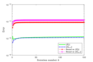
Refer to caption

(a)

Refer to caption

(b)

Refer to caption

(c)

Refer to caption

(d)

Fig. 3: Estimated error bounds for F^knormsubscript^𝐹𝑘\|\widehat{F}_{k}\| and G^knormsubscript^𝐺𝑘\|\widehat{G}_{k}\|: (a) {Acsubscript𝐴𝑐A_{c}, Lssubscript𝐿𝑠L_{s}}; (b) {well1850, L1subscript𝐿1L_{1}}; (c) {rdb2048, dw2048}; (d) {c-23, Lnsubscript𝐿𝑛L_{n}}.

Figure 3 depicts the growths of F^knormsubscript^𝐹𝑘\|\widehat{F}_{k}\| and G^knormsubscript^𝐺𝑘\|\widehat{G}_{k}\| in (44) and (45). By Theorem 3, we take O(B¯k1ϵ)=10B¯k1ϵO(\lVert\underline{B}_{k}^{-1}\lVert\epsilon)=10\lVert\underline{B}_{k}^{-1}\lVert\epsilon and O((B¯k1+B^k1)ϵ)=10(B¯k1+B^k1)ϵO((\lVert\underline{B}_{k}^{-1}\lVert+\|\widehat{B}_{k}^{-1}\|)\epsilon)=10(\lVert\underline{B}_{k}^{-1}\lVert+\|\widehat{B}_{k}^{-1}\|)\epsilon, respectively. From the figures, we see that O(B¯k1ϵ)O(\lVert\underline{B}_{k}^{-1}\lVert\epsilon) and O((B¯k1+B^k1)ϵ)O((\lVert\underline{B}_{k}^{-1}\lVert+\|\widehat{B}_{k}^{-1}\|)\epsilon) are indeed reasonable upper bounds for F^knormsubscript^𝐹𝑘\|\widehat{F}_{k}\| and G^knormsubscript^𝐺𝑘\|\widehat{G}_{k}\|, and the growths of F^knormsubscript^𝐹𝑘\|\widehat{F}_{k}\| and G^knormsubscript^𝐺𝑘\|\widehat{G}_{k}\| are critically affected by those of B¯k1\lVert\underline{B}_{k}^{-1}\lVert and B¯k1+B^k1\lVert\underline{B}_{k}^{-1}\lVert+\|\widehat{B}_{k}^{-1}\|, respectively. For the four matrix pairs, B¯k1\lVert\underline{B}_{k}^{-1}\lVert always grows slowly, but B^k1=B¯k1normsuperscriptsubscript^𝐵𝑘1normsuperscriptsubscript¯𝐵𝑘1\|\widehat{B}_{k}^{-1}\|=\|\bar{B}_{k}^{-1}\| grows faster for {well1850, L1subscript𝐿1L_{1}} than for the other three pairs. This is because L1subscript𝐿1L_{1} is truly flat and the smallest singular value of B¯ksubscript¯𝐵𝑘\bar{B}_{k} converges to zero as k𝑘k increases, causing that B¯k1normsuperscriptsubscript¯𝐵𝑘1\|\bar{B}_{k}^{-1}\| is ultimately very large, as we have shown in almost one page after Theorem 1; in contrast, the smallest singular value of B¯ksubscript¯𝐵𝑘\bar{B}_{k} converges to the nonzero smallest one of L𝐿L for the other three matrix pairs, and B¯k1normsuperscriptsubscript¯𝐵𝑘1\|\bar{B}_{k}^{-1}\| is uniformly bounded by the reciprocal of the smallest singular value of L𝐿L.

Refer to caption

(a)

Refer to caption

(b)

Refer to caption

(c)

Refer to caption

(d)

Fig. 4: Orthogonality level of U^ksubscript^𝑈𝑘\widehat{U}_{k}: (a) {Acsubscript𝐴𝑐A_{c}, Lssubscript𝐿𝑠L_{s}}; (b) {well1850, L1subscript𝐿1L_{1}}; (c) {rdb2048, dw2048}; (d) {c-23, Lnsubscript𝐿𝑛L_{n}}.

Figure 4 depicts the orthogonality level of U^ksubscript^𝑈𝑘\widehat{U}_{k} measured by η(U^k)𝜂subscript^𝑈𝑘\eta(\widehat{U}_{k}) as k𝑘k increases from 111 to 150150150. The upper bound for η(U^k)𝜂subscript^𝑈𝑘\eta(\widehat{U}_{k}) is (51), and we use 10ϵ10italic-ϵ10\epsilon as an estimate for O(c3(m,n,p)ϵ)𝑂subscript𝑐3𝑚𝑛𝑝italic-ϵO(c_{3}(m,n,p)\epsilon). We observe that the orthogonality of U^ksubscript^𝑈𝑘\widehat{U}_{k} will lose gradually. Particularly, for the test problem {rdb2048, dw2048}, the columns of U^ksubscript^𝑈𝑘\widehat{U}_{k} lose orthogonality completely and become numerically linearly dependent after k=100𝑘100k=100. The growth trends of η(U^k)𝜂subscript^𝑈𝑘\eta(\widehat{U}_{k}) and its bound resemble, meaning that the orthogonality level of U^ksubscript^𝑈𝑘\widehat{U}_{k} is affected not only by η(Uk)𝜂subscript𝑈𝑘\eta(U_{k}) and η(V~k)𝜂subscript~𝑉𝑘\eta(\tilde{V}_{k}) but also by B^k1normsuperscriptsubscript^𝐵𝑘1\|\widehat{B}_{k}^{-1}\|.

5.2 Examples for the GSVD computation

We illustrate the numerical performance of the JBD method for computing a few extreme GSVD components of {A,L}𝐴𝐿\{A,L\}. We will show the convergence behavior of the computed Ritz values and vectors, and justify the upper bound in (63).

Example 1. We show the convergence of the singular values, the computed Ritz values, of Bksubscript𝐵𝑘B_{k} or B¯ksubscript¯𝐵𝑘\bar{B}_{k}. Take m=n=p=500𝑚𝑛𝑝500m=n=p=500, and construct a row vector c=(c1,,cn)𝑐subscript𝑐1subscript𝑐𝑛c=(c_{1},\ldots,c_{n}) with lmax=4,lmin=2,c(1:lmax)=linspace(0.99,0.7,lmax),c(nlmin+1:n)=linspace(0.10,0.01,lmin),c(lmax+1:nlmin)=linspace(0.65,0.15,nlmaxlmin)formulae-sequencesubscript𝑙4formulae-sequencesubscript𝑙2formulae-sequencesubscript𝑐:1subscript𝑙linspace0.990.7subscript𝑙formulae-sequencesubscript𝑐:𝑛subscript𝑙1𝑛linspace0.100.01subscript𝑙subscript𝑐:subscript𝑙1𝑛subscript𝑙linspace0.650.15𝑛subscript𝑙subscript𝑙l_{\max}=4,l_{\min}=2,c_{(1:l_{\max})}=\texttt{linspace}(0.99,0.7,l_{\max}),c_{(n-l_{\min}+1:n)}=\texttt{linspace}(0.10,0.01,l_{\min}),c_{(l_{\max}+1:n-l_{\min})}=\texttt{linspace}(0.65,0.15,n-l_{\max}-l_{\min}) and s=(1c12,,1cn2),𝑠1superscriptsubscript𝑐121superscriptsubscript𝑐𝑛2s=(\sqrt{1-c_{1}^{2}},\ldots,\sqrt{1-c_{n}^{2}}), where linspace is the Matlab built-in function. Then define CA=diag(c)subscript𝐶𝐴diag𝑐C_{A}=\mathop{\operator@font diag}\nolimits(c), SL=diag(s)subscript𝑆𝐿diag𝑠S_{L}=\mathop{\operator@font diag}\nolimits(s) and D = gallery(‘orthog’,n,2), and take A=CAD𝐴subscript𝐶𝐴𝐷A=C_{A}D and L=SLD𝐿subscript𝑆𝐿𝐷L=S_{L}D. By construction, κ(A)=6.6000𝜅𝐴6.6000\kappa(A)=6.6000 and κ(L)=7.0888𝜅𝐿7.0888\kappa(L)=7.0888, the i𝑖i-th large generalized singular value pair of {A,L}𝐴𝐿\{A,L\} is {ci,si}subscript𝑐𝑖subscript𝑠𝑖\{c_{i},s_{i}\}.

Refer to caption

(a)

Refer to caption

(b)

Refer to caption

(c)

Refer to caption

(d)

Fig. 5: Convergence of Ritz values computed by the SVD of Bksubscript𝐵𝑘B_{k}: (a) the first six largest Ritz values without reorthogonalization; (b) the first six largest Ritz values with full reorthogonalization; (c) the first six smallest Ritz values without reorthogonalization; (d) the first six smallest Ritz values with full reorthogonalization.

Figure 5 depicts the convergence processes of the first six largest and smallest Ritz values computed by the SVD of Bksubscript𝐵𝑘B_{k}, respectively, where we implemented the JBD process without and with reorthogonalization. The right vertical line indicates the values of cisubscript𝑐𝑖c_{i} for i=1,,500𝑖1500i=1,\dots,500, and the left and right panels exhibit the convergence behaviors of the JBD method without and with reorthogonalization. We observe from Figure 5(a) and Figure 5(c) that some of the converged Ritz values suddenly jump to become a ghost and then converge to the next large or small singular values after several iterations. Such a phenomenon repeats several times and corresponds to spurious copies each time. More precisely, as Figure 5(a) indicates, the six largest Ritz values gradually become numerically multiple and ultimately converge to the single largest generalized singular value of {A,L}𝐴𝐿\{A,L\} as k𝑘k increases, of which five ones are ghosts. Similarly, as Figure 5 (c) shows, the six smallest Ritz values ultimately converge to the two smallest generalized singular values of {A,L}𝐴𝐿\{A,L\}, of which the most slowly converged Ritz value first converges to the seventh smallest generalized singular value of {A,L}𝐴𝐿\{A,L\}, then suddenly jumps and starts to approximate the smallest one after 69 iterations, and the other five Ritz values finally become numerically multiple and converge to the second smallest generalized singular value of {A,L}𝐴𝐿\{A,L\} after nearly 170 iterations, meaning that four of these five ones are ghosts since then.

However, when the JBD process is performed with full reorthogonalization, the convergence of the Ritz values changes and becomes regular, as Figure 5(b) and Figure 5(d) indicate. In the right panels, the convergence behavior is much simpler and is in accordance with theoretical analysis in exact arithmetic. It is clear that a simple generalized singular value is approximated by Ritz values without ghosts. We also observe from both the panels that the extreme Ritz values converge more quickly than relatively interior Ritz values, that is, the Ritz values closer to the right-most or left-most generalized singular values stabilize more early, which confirms the theory that the JBD method generally favors the extreme generalized singular values.
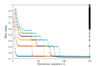
Refer to caption

(a)

Refer to caption

(b)

Fig. 6: Convergence of Ritz values computed by the SVD of B¯ksubscript¯𝐵𝑘\bar{B}_{k}: (a) the first six smallest Ritz values without reorthogonalization; (b) the first six smallest Ritz values with full reorthogonalization.

Figure 6 depicts the convergence processes of the first six smallest Ritz values computed by the SVD of B¯ksubscript¯𝐵𝑘\bar{B}_{k}, which corresponds to the first largest generalized singular values of {A,L}𝐴𝐿\{A,L\}. The convergence behavior of the largest Ritz values by the SVD of B¯ksubscript¯𝐵𝑘\bar{B}_{k} is similar and thus omitted. The right vertical line indicates the values of sisubscript𝑠𝑖s_{i} for i=1,,500𝑖1500i=1,\dots,500. From Figure 6(a), we observe the “ghost” phenomenon that some converged Ritz values suddenly jump and then converge to the next small singular values after several iterations. More detailed convergence phenomena are similar to Figure 5(a) and Figure 5(c). Figure 6(b) shows the convergence of Ritz values with full reorthogonalization, from which it is clear that the JBD method converges regularly and there are no spurious copies. Figure 6(a)–Figure 6(b) demonstrate that the JBD method favors the extreme generalized singular values.

Example 2. We investigate the convergence of the approximate generalized singular values and vectors of {A,L}𝐴𝐿\{A,L\}, which are computed by using both the SVDs of Bksubscript𝐵𝑘B_{k} and B¯ksubscript¯𝐵𝑘\bar{B}_{k} and the GSVD of {Bk,B¯k}subscript𝐵𝑘subscript¯𝐵𝑘\{B_{k},\bar{B}_{k}\}. We test two matrix pairs. The first pair is the problem in Example 1, and the second pair {dw256A,dw256B}𝑑𝑤256𝐴𝑑𝑤256𝐵\{dw256A,dw256B\} is an electromagnetic problem with m=n=p=512𝑚𝑛𝑝512m=n=p=512 from the non-Hermitian Eigenvalue Problem Collection in the Matrix Market333https://math.nist.gov/MatrixMarket, where κ(A)=11490.4𝜅𝐴11490.4\kappa(A)=11490.4 and κ(L)=3.7328𝜅𝐿3.7328\kappa(L)=3.7328.

We use the JBD method with full reorthogonalization to compute the largest generalized singular value and vectors. Instead of the SVD of the individual Bksubscript𝐵𝑘B_{k} or B¯ksubscript¯𝐵𝑘\bar{B}_{k}, we compute the SVDs of Bksubscript𝐵𝑘B_{k} and B¯ksubscript¯𝐵𝑘\bar{B}_{k} simultaneously, and take {c1(k),s¯1(k)}superscriptsubscript𝑐1𝑘superscriptsubscript¯𝑠1𝑘\{c_{1}^{(k)},\bar{s}_{1}^{(k)}\} to approximate {c1,s1}subscript𝑐1subscript𝑠1\{c_{1},s_{1}\}, where c1(k)superscriptsubscript𝑐1𝑘c_{1}^{(k)} is the largest singular value of Bksubscript𝐵𝑘B_{k} and s¯1(k)superscriptsubscript¯𝑠1𝑘\bar{s}_{1}^{(k)} is the smallest singular value of B¯ksubscript¯𝐵𝑘\bar{B}_{k}. The approximations to the right and left generalized singular vectors x1subscript𝑥1x_{1} and p1Asuperscriptsubscript𝑝1𝐴p_{1}^{A} are computed from the SVD of Bksubscript𝐵𝑘B_{k}, and the approximation to the left generalized singular vectors p1Lsuperscriptsubscript𝑝1𝐿p_{1}^{L} is computed from the SVD of B¯ksubscript¯𝐵𝑘\bar{B}_{k}. Alternatively, we also compute the largest GSVD components of these two matrix pairs using the GSVD of {Bk,B¯k}subscript𝐵𝑘subscript¯𝐵𝑘\{B_{k},\bar{B}_{k}\} and obtain the approximation {c1(k),s1(k)}superscriptsubscript𝑐1𝑘superscriptsubscript𝑠1𝑘\{c_{1}^{(k)},s_{1}^{(k)}\} to {c1,s1}subscript𝑐1subscript𝑠1\{c_{1},s_{1}\} and the approximations x1(k),y1(k),z1(k)superscriptsubscript𝑥1𝑘superscriptsubscript𝑦1𝑘superscriptsubscript𝑧1𝑘x_{1}^{(k)},y_{1}^{(k)},z_{1}^{(k)} to x1,p1A,p1Lsubscript𝑥1superscriptsubscript𝑝1𝐴superscriptsubscript𝑝1𝐿x_{1},p_{1}^{A},p_{1}^{L}.

We use the angle error

sinθk=|s¯1(k)c1s1c1(k)| or |s1(k)c1s1c1(k)|subscript𝜃𝑘superscriptsubscript¯𝑠1𝑘subscript𝑐1subscript𝑠1superscriptsubscript𝑐1𝑘 or superscriptsubscript𝑠1𝑘subscript𝑐1subscript𝑠1superscriptsubscript𝑐1𝑘\sin\theta_{k}=|\bar{s}_{1}^{(k)}c_{1}-s_{1}c_{1}^{(k)}|\mbox{ or }|s_{1}^{(k)}c_{1}-s_{1}c_{1}^{(k)}|

to measure the error between {c1(k),s¯1(k)}superscriptsubscript𝑐1𝑘superscriptsubscript¯𝑠1𝑘\{c_{1}^{(k)},\bar{s}_{1}^{(k)}\} or {c1(k),s1(k)}superscriptsubscript𝑐1𝑘superscriptsubscript𝑠1𝑘\{c_{1}^{(k)},s_{1}^{(k)}\} and {c1,s1}subscript𝑐1subscript𝑠1\{c_{1},s_{1}\} [34], where θksubscript𝜃𝑘\theta_{k} denotes the angle between the vectors (c1,s1)Tsuperscriptsubscript𝑐1subscript𝑠1𝑇(c_{1},s_{1})^{T} and (c1(k),s¯1(k))Tsuperscriptsuperscriptsubscript𝑐1𝑘superscriptsubscript¯𝑠1𝑘𝑇(c_{1}^{(k)},\bar{s}_{1}^{(k)})^{T} or (c1(k),s1(k))Tsuperscriptsuperscriptsubscript𝑐1𝑘superscriptsubscript𝑠1𝑘𝑇(c_{1}^{(k)},s_{1}^{(k)})^{T}. For the corresponding generalized singular vectors, we measure the errors
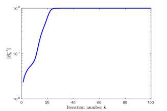
sin(x1,x1(k)),sin(p1A,y1(k)),sin(p1L,z1(k)).subscript𝑥1superscriptsubscript𝑥1𝑘superscriptsubscript𝑝1𝐴superscriptsubscript𝑦1𝑘superscriptsubscript𝑝1𝐿superscriptsubscript𝑧1𝑘\sin\angle(x_{1},x_{1}^{(k)}),\ \ \sin\angle(p_{1}^{A},y_{1}^{(k)}),\ \ \sin\angle(p_{1}^{L},z_{1}^{(k)}).

Refer to caption

(a)

Refer to caption

(b)

Refer to caption

(c)

Refer to caption

(d)

Fig. 7: Growth of B¯k1normsuperscriptsubscript¯𝐵𝑘1\|\underline{B}_{k}^{-1}\| and B^k1normsuperscriptsubscript^𝐵𝑘1\|\widehat{B}_{k}^{-1}\|: (a),(b) {A500subscript𝐴500A_{500}, L500subscript𝐿500L_{500}} in Example 1; (c),(d) {dw256A,256B𝑑𝑤256𝐴256𝐵dw256A,256B} in Example 2.

Refer to caption

(a)

Refer to caption

(b)

Fig. 8: Convergence processes of the approximate GSVD components: (a) {A500subscript𝐴500A_{500}, L500subscript𝐿500L_{500}} in Example 1; (b) {dw256A,256B𝑑𝑤256𝐴256𝐵dw256A,256B} in Example 2.

Figure 8 draws the approximation processes of the approximate generalized singular values and vectors obtained by the SVDs of Bksubscript𝐵𝑘B_{k} and B¯ksubscript¯𝐵𝑘\bar{B}_{k} as k𝑘k increases, while Figure 7 depicts the growths of B¯k1normsuperscriptsubscript¯𝐵𝑘1\|\underline{B}_{k}^{-1}\| and B^k1normsuperscriptsubscript^𝐵𝑘1\|\widehat{B}_{k}^{-1}\|. We have found that, for these two matrix pairs, B¯k1normsuperscriptsubscript¯𝐵𝑘1\|\underline{B}_{k}^{-1}\| and B^k1normsuperscriptsubscript^𝐵𝑘1\|\widehat{B}_{k}^{-1}\| grow quite slowly and are very modest for Example 1 when k=1150𝑘1similar-to150k=1\sim 150 and for Example 2 when k=1150𝑘1similar-to150k=1\sim 150, respectively. The approximate GSVD components converge regularly, the JBD method converges fast, and all the errors achieve the level of ϵitalic-ϵ\epsilon after twenty iterations for Example 1.

Figure 9 depicts the convergence processes of approximate GSVD components computed by the GSVD of {Bk,B¯k}subscript𝐵𝑘subscript¯𝐵𝑘\{B_{k},\bar{B}_{k}\}. In this figure, we also draw the curves of residual norms. Clearly, the computed results are very similar to those obtained by the SVDs of Bksubscript𝐵𝑘B_{k} and B¯ksubscript¯𝐵𝑘\bar{B}_{k} until the errors reach the level of ϵitalic-ϵ\epsilon.

Refer to caption

(a)

Refer to caption

(b)

Fig. 9: Convergence processes of the approximate GSVD components based on the GSVD of {Bk,B¯k}subscript𝐵𝑘subscript¯𝐵𝑘\{B_{k},\bar{B}_{k}\}: (a) {A500subscript𝐴500A_{500}, L500subscript𝐿500L_{500}} in Example 1; (b) {dw256A,dw256B}.

Example 3. We show the residual norm and its upper bound (63). The matrix pair {A,L}𝐴𝐿\{A,L\} is chosen to be {A800,L800}subscript𝐴800subscript𝐿800\{A_{800},L_{800}\} in Table 1, and we use the largest singular value of Bksubscript𝐵𝑘B_{k} to compute an approximation to the largest generalized singular value. From the construction, we have (A800T,L800T)T=1normsuperscriptsuperscriptsubscript𝐴800𝑇superscriptsubscript𝐿800𝑇𝑇1\|(A_{800}^{T},L_{800}^{T})^{T}\|=1, and the largest generalized singular value is {c1,s1}subscript𝑐1subscript𝑠1\{c_{1},s_{1}\}, where c1=0.75subscript𝑐10.75c_{1}=0.75 and s1=1c12subscript𝑠11superscriptsubscript𝑐12s_{1}=\sqrt{1-c_{1}^{2}}.

We also display the convergence processes of the approximate generalized singular values by using both the angle error and relative error
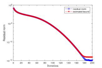
|c1(k)/s1(k)c1/s1|/(c1/s1).superscriptsubscript𝑐1𝑘superscriptsubscript𝑠1𝑘subscript𝑐1subscript𝑠1subscript𝑐1subscript𝑠1|c_{1}^{(k)}/s_{1}^{(k)}-c_{1}/s_{1}|/(c_{1}/s_{1}).

Refer to caption

(a)

Refer to caption

(b)

Fig. 10: Convergence history of the approximate largest generalized singular value of {A800,L800}subscript𝐴800subscript𝐿800\{A_{800},L_{800}\}: (a) residual norm and its upper bound; (b) angle error and relative error.

We draw the convergence histories of the approximate largest generalized singular value and the residual norm in Figure 10. From Figure 10(b), It is found that the approximate largest generalized singular value c1(k)/s1(k)superscriptsubscript𝑐1𝑘superscriptsubscript𝑠1𝑘c_{1}^{(k)}/s_{1}^{(k)} converges to c1/s1subscript𝑐1subscript𝑠1c_{1}/s_{1}, and the relative error curve shows that the approximation accuracy of ci(k)/si(k)superscriptsubscript𝑐𝑖𝑘superscriptsubscript𝑠𝑖𝑘c_{i}^{(k)}/s_{i}^{(k)} to ci/sisubscript𝑐𝑖subscript𝑠𝑖c_{i}/s_{i} reaches O(ϵ)𝑂italic-ϵO(\epsilon). We observe from Figure 10(a) that the residual norm and its upper bound are almost the same as k𝑘k increases. The true residual norm decays until the level of ϵitalic-ϵ\epsilon, but the estimated upper bound stagnates at the level that is a little bit higher than ϵitalic-ϵ\epsilon, since the upper bound for ri(k)normsuperscriptsubscript𝑟𝑖𝑘\|r_{i}^{(k)}\| has a term O(B¯k1ϵ)𝑂normsuperscriptsubscript¯𝐵𝑘1italic-ϵO(\|\underline{B}_{k}^{-1}\|\epsilon), which is considerably bigger than ϵitalic-ϵ\epsilon when B¯k1>1normsuperscriptsubscript¯𝐵𝑘11\|\underline{B}_{k}^{-1}\|>1 considerably. For the case that B¯k1normsuperscriptsubscript¯𝐵𝑘1\|\underline{B}_{k}^{-1}\| remains modest, the term O(B¯k1ϵ)𝑂normsuperscriptsubscript¯𝐵𝑘1italic-ϵO(\|\underline{B}_{k}^{-1}\|\epsilon) plays no role in the upper bound until the bound reaches O(ϵ)𝑂italic-ϵO(\epsilon). Therefore, the upper bound Rαk+1βk+1|ekTwi(k)|norm𝑅subscript𝛼𝑘1subscript𝛽𝑘1superscriptsubscript𝑒𝑘𝑇superscriptsubscript𝑤𝑖𝑘\|R\|\alpha_{k+1}\beta_{k+1}|e_{k}^{T}w_{i}^{(k)}| can be used as a reliable stopping criterion for the JBD algorithm. We have seen that the angle errors and relative errors resemble very much, as is expected since c1/s1=O(1)subscript𝑐1subscript𝑠1𝑂1c_{1}/s_{1}=O(1). We point out that, in large matrix computations, a (relative) stopping tolerance is usually O(ϵ1/2)𝑂superscriptitalic-ϵ12O(\epsilon^{1/2}). Therefore, provided that B¯k1O(ϵ1/2)normsuperscriptsubscript¯𝐵𝑘1𝑂superscriptitalic-ϵ12\|\underline{B}_{k}^{-1}\|\leq O(\epsilon^{-1/2}), our upper bound is a very reliable estimate for ri(k)normsuperscriptsubscript𝑟𝑖𝑘\|r_{i}^{(k)}\|.

6 Conclusions and future work

We have made a numerical analysis of the JBD process on {A,L}𝐴𝐿\{A,L\} in finite precision, and established relationships between it and respective lower and upper Lanczos bidiagonalizations of QAsubscript𝑄𝐴Q_{A} and QLsubscript𝑄𝐿Q_{L} in the presence of round-offs. The results have shown that the k𝑘k-step JBD process for computing Uk+1subscript𝑈𝑘1U_{k+1}, Vksubscript𝑉𝑘V_{k} and Bksubscript𝐵𝑘B_{k} is equivalent to the lower Lanczos bidiagonalization of QAsubscript𝑄𝐴Q_{A} with the error δ=O(B¯k1ϵ)\delta=O(\lVert\underline{B}_{k}^{-1}\lVert\epsilon), and it for computing U^k+1subscript^𝑈𝑘1\widehat{U}_{k+1}, Vksubscript𝑉𝑘V_{k} and B^ksubscript^𝐵𝑘\widehat{B}_{k} is equivalent to the upper Lanczos bidiagonalization of QLsubscript𝑄𝐿Q_{L} with the error δ^=O((B¯k1+B^k1)ϵ)^𝛿𝑂normsuperscriptsubscript¯𝐵𝑘1normsuperscriptsubscript^𝐵𝑘1italic-ϵ\hat{\delta}=O((\|\underline{B}_{k}^{-1}\|+\|\widehat{B}_{k}^{-1}\|)\epsilon). We have investigated the loss of orthogonality of the computed basis vectors and established an upper bound for the orthogonality level of η(U^k)𝜂subscript^𝑈𝑘\eta(\widehat{U}_{k}), showing that its orthogonality level is controlled by those of Uk+1subscript𝑈𝑘1U_{k+1}, V~ksubscript~𝑉𝑘\widetilde{V}_{k}, i.e., Vksubscript𝑉𝑘V_{k}, and the quantity B^k1normsuperscriptsubscript^𝐵𝑘1\|\widehat{B}_{k}^{-1}\|.

We have shown how to use the JBD process to compute a few extreme generalized singular values and vectors of {A,L}𝐴𝐿\{A,L\} and proposed a JBD method that obtains approximate generalized singular values and vectors using a few computational approaches, which include three approaches to obtain approximate generalized singular values and approximate right generalized singular vectors by computing the SVDs of Bksubscript𝐵𝑘B_{k} and B¯ksubscript¯𝐵𝑘\bar{B}_{k} and the GSVD of {Bk,B¯k}subscript𝐵𝑘subscript¯𝐵𝑘\{B_{k},\bar{B}_{k}\} and two approaches to obtain approximate left generalized singular vectors of A𝐴A and L𝐿L by computing either the left singular vectors of Bksubscript𝐵𝑘B_{k} and B¯ksubscript¯𝐵𝑘\bar{B}_{k} simultaneously or the left generalized singular vectors of {Bk,B¯k}subscript𝐵𝑘subscript¯𝐵𝑘\{B_{k},\bar{B}_{k}\}. We have considered the convergence and accuracy of the approximate generalized singular values. The results have indicated that the generalized singular values of Bksubscript𝐵𝑘B_{k} and B¯ksubscript¯𝐵𝑘\bar{B}_{k} are as accurate as the true Ritz values of QAsubscript𝑄𝐴Q_{A} and QLsubscript𝑄𝐿Q_{L} with respect to the given subspaces within 𝒪(ϵ)𝒪italic-ϵ\mathcal{O}(\epsilon), provided that the basis vectors have semiorthogonality levels and B¯ksubscript¯𝐵𝑘\underline{B}_{k} and B¯ksubscript¯𝐵𝑘\bar{B}_{k} are not ill conditioned. Under these conditions, it is only necessary to maintain the desired semiorthogonality in order to obtain the approximate GSVD components with the same accuracy as those obtained by the JBD method with full reorthogonalization. An efficient partial reorthogonalization strategy has been proposed in [12] for this purpose.

In the meantime, we have established a compact upper bound for the residual norm ri(k)normsuperscriptsubscript𝑟𝑖𝑘\|r_{i}^{(k)}\| of an approximate generalized singular value and approximate right generalized singular vector in finite precision and shown that it can be used as a cheap and reliable stopping criterion without explicitly computing the approximate right generalized singular vector until the convergence occurs. Finally, we have reported numerical experiments to justify all the results obtained and assertions.

There remain some important issues. For instance, due to the limitation of storage, it is generally necessary to restart the JBD method. A commonly used restarting technique is the implicit restarting proposed in [33] for the eigenvalue problem and adapted to the SVD computation in [13, 14, 19]. How to adapt the implicit restart to the JBD method and develop efficient algorithms is very significant. Also, notice that the residual norm (61) is used to measure the convergence of the JBD method, which is the residual norm of an approximate generalized eigenpair ((ci(k)/si(k))2,xi(k))superscriptsuperscriptsubscript𝑐𝑖𝑘superscriptsubscript𝑠𝑖𝑘2superscriptsubscript𝑥𝑖𝑘((c_{i}^{(k)}/s_{i}^{(k)})^{2},x_{i}^{(k)}) of si2ATAxi=ci2LTLxisuperscriptsubscript𝑠𝑖2superscript𝐴𝑇𝐴subscript𝑥𝑖superscriptsubscript𝑐𝑖2superscript𝐿𝑇𝐿subscript𝑥𝑖s_{i}^{2}A^{T}Ax_{i}=c_{i}^{2}L^{T}Lx_{i} and does not take approximate left generalized singular vectors yi(k)superscriptsubscript𝑦𝑖𝑘y_{i}^{(k)} for A𝐴A and zi(k)superscriptsubscript𝑧𝑖𝑘z_{i}^{(k)} for L𝐿L into account. A much more proper criterion is to measure the residual norm of the approximate GSVD components (ci(k),si(k),xi(k),yi(k),zi(k))superscriptsubscript𝑐𝑖𝑘superscriptsubscript𝑠𝑖𝑘superscriptsubscript𝑥𝑖𝑘superscriptsubscript𝑦𝑖𝑘superscriptsubscript𝑧𝑖𝑘(c_{i}^{(k)},s_{i}^{(k)},x_{i}^{(k)},y_{i}^{(k)},z_{i}^{(k)}), which, by the definition (8) of GSVD of {A,L}𝐴𝐿\{A,L\}, is

ri(k)=Axi(k)ci(k)yi(k)2+Lxi(k)si(k)zi(k)2+si(k)ATyi(k)ci(k)LTzi(k)2.normsuperscriptsubscript𝑟𝑖𝑘superscriptnorm𝐴superscriptsubscript𝑥𝑖𝑘superscriptsubscript𝑐𝑖𝑘superscriptsubscript𝑦𝑖𝑘2superscriptnorm𝐿superscriptsubscript𝑥𝑖𝑘superscriptsubscript𝑠𝑖𝑘superscriptsubscript𝑧𝑖𝑘2superscriptnormsuperscriptsubscript𝑠𝑖𝑘superscript𝐴𝑇superscriptsubscript𝑦𝑖𝑘superscriptsubscript𝑐𝑖𝑘superscript𝐿𝑇superscriptsubscript𝑧𝑖𝑘2\|r_{i}^{(k)}\|=\sqrt{\|Ax_{i}^{(k)}-c_{i}^{(k)}y_{i}^{(k)}\|^{2}+\|Lx_{i}^{(k)}-s_{i}^{(k)}z_{i}^{(k)}\|^{2}+\|s_{i}^{(k)}A^{T}y_{i}^{(k)}-c_{i}^{(k)}L^{T}z_{i}^{(k)}\|^{2}}.

We need to establish reliable upper bounds for it in exact arithmetic and in finite precision so as to design an efficient stopping criterion for the GSVD computation.

References

  • [1] J. L. Barlow, Reorthogonalization for the Golub-Kahan-Lanczos bidiagonal reduction, Numer. Math., 124 (2013), pp. 237–278.
  • [2] Å. Björck, Numerical Methods for Least Squares Problems, SIAM, Philadelphia, PA, 1996.
  • [3] T. A. Davis and Y. Hu, The University of Florida sparse matrix collection, ACM Trans. Math. Software, 38 (2011), pp. 1–-25. Data available from \urlhttp://www.cise.ufl.edu/research/sparse/matrices/.
  • [4] G. H. Golub and W. Kahan, Calculating the singular values and pseudo-inverse of a matrix, SIAM J. Numer. Anal., 2 (1965), pp. 205–224.
  • [5] G. H. Golub and C. F. Van Loan, Matrix Computations, 4th ed., The Johns Hopkins University Press, 2013.
  • [6] P. C. Hansen, Rank-Deficient and Discrete Ill-Posed Problems: Numerical Aspects of Linear Inversion, SIAM, Philadelphia, PA, 1998.
  • [7] P. C. Hansen, Discrete Inverse Problems: Insight and Algorithms, SIAM, Philadelphia, PA, 2010.
  • [8] N. J. Higham, Accuracy and Stability of Numerical Algorithms, 2nd ed., SIAM, Philadelphia, PA, 2002.
  • [9] Z. Jia, The low rank approximations and Ritz values in LSQR for linear discrete ill-posed problem, Inverse Probl., 36 (2020), 045013 (31pp).
  • [10] Z. Jia, Regularization properties of LSQR for linear discrete ill-posed problems in the multiple singular value case and best, near best and general low rank approximations, Inverse Probl., 36 (2020), 085009 (38pp).
  • [11] Z. Jia, Regularization properties of Krylov iterative solvers CGME and LSMR for linear dicrete ill-posed problems with an application to truncated randomized SVDs, Numer. Algor., 85 (2020), pp. 1281–1310.
  • [12] Z. Jia and H. Li, The joint bidiagonalization process with partial reorthogonalization, Numer. Algor., 88 (2021), pp. 965–992.
  • [13] Z. Jia and D. Niu, An implicitly restarted refined bidiagonalization Lanczos method for computing a partial singular value decomposition, SIAM J. Matrix Anal. Appl., 25 (2003), pp. 246–265.
  • [14] Z. Jia and D. Niu, A refined harmonic Lanczos bidiagonalization method and an implicitly restarted algorithm for computing the smallest singular triplets of large matrices, SIAM J. Sci. Comput., 32 (2010), pp. 714–744.
  • [15] Z. Jia and Y. Yang, A joint bidiagonalization based algorithm for large scale general-form Tikhonov regularization, Appl. Numer. Math., 157 (2020), pp. 159–177.
  • [16] M. E. Kilmer, P. C. Hansen, AND M. I. Español, A projection-based approach to general-form Tikhonov regularization, SIAM J. Sci. Comput., 29 (2007), pp. 315–330.
  • [17] C. Lanczos, An iteration method for the solution of eigenvalue problem of linear differential and integral operators, J. Res. Nat. Bur, 45 (1950), pp. 255–282.
  • [18] R. M. Larsen, Lanczos bidiagonalization with partial reorthogonalization, Department of Computer Science, University of Aarhus, 1998.
  • [19] R. M. Larsen, Combining implicit restarts and partial reorthogonalization in Lanczos bidiagonalization, SCCM, Stanford University, (2001).
  • [20] G. Meurant and Z. Strakoš, The Lanczos and conjugate gradient algorithms in finite precision arithmetic, Acta Numer., 15 (2006), pp. 471–542.
  • [21] C. C. Paige, The computation of eigenvalues and eigenvectors of very large sparse matrices, PhD thesis, London University, London, England, 1971.
  • [22] C. C. Paige, Computational variants of the Lanczos method for the eigenproblem, J. Inst. Math. Appl., 10 (1972), pp. 373–381.
  • [23] C. C. Paige, Error analysis of the Lanczos algorithm for tridiagonalizing a symmetric matrix, J. Inst. Math. Appl., 18 (1976), pp. 341–349.
  • [24] C. C. Paige, Accuracy and effectiveness of the Lanczos algorithm for the symmetric eigenproblem, Linear Algebra Appl., 34 (1980), pp. 235–258.
  • [25] C. C. Paige and M. A. Saunders, Towards a generalized singular value decomposition, SIAM J. Numer. Anal., 18 (1981), pp. 398–405.
  • [26] C. C. Paige and M. A. Saunders, LSQR: an algorithm for sparse linear equations and sparse least squares, ACM Trans. Math. Soft., 8 (1982), pp. 43–71.
  • [27] B. N. Parlett, The Symmetric Eigenvalue Problem, SIAM, Philadelphia, PA, 1998.
  • [28] B. N. Parlett and D. S. Scott, The Lanczos algorithm with selective orthogonalization, Math. Comput., 33 (1979), pp. 217–238.
  • [29] Y. Saad, On the rates of convergence of the Lanczos and the block-Lanczos methods, SIAM J. Numer. Anal., 17 (1980), pp. 687–706.
  • [30] H. D. Simon, Analysis of the symmetric Lanczos algorithm with reorthogonalization methods, Linear Algebra Appl., 61 (1984), pp. 101–131.
  • [31] H. D. Simon, The Lanczos algorithm with partial reorthogonalization, Math. Comput., 42 (1984), pp. 115–142.
  • [32] H. D. Simon and H. Zha, Low-rank matrix approximation using the Lanczos bidiagonalization process with applications, SIAM J. Sci. Comput., 21 (2000), pp. 2257–2274.
  • [33] D. C. Sorensen, Implicit application of polynomial filters in a k-step Arnoldi method, SIAM J. Matrix Anal. Appl., 13 (1992), pp. 357–385.
  • [34] J.-G. Sun, Perturbation analysis for the generalized singular value problem, SIAM J. Numer. Anal., 20 (1983), pp. 611–625.
  • [35] C. F. Van Loan, Generalizing the singular value decompositions, SIAM J. Numer. Anal., 13 (1976), pp. 76–83.
  • [36] C. F. Van Loan, Computing the CS and generalized singular value decomposition, Numer. Math., 46 (1985), pp. 479–491.
  • [37] H. Zha, Computing the generalized singular values/vectors of large sparse or structured matrix pairs, Numer. Math., 72 (1996), pp. 391–417.