Lambda-Policy Iteration with Randomization for Contractive Models
with Infinite Policies: Well-Posedness and Convergence
(Extended Version)

\NameYuchao Li \Emailyuchao@kth.se
\NameKarl H. Johansson \Emailkallej@kth.se
\NameJonas Mårtensson \Emailjonas1@kth.se
\addrDivision of Decision and Control Systems
   KTH Royal Institute of Technology    Stockholm    Sweden
Abstract

Abstract dynamic programming models are used to analyze λ𝜆\lambda-policy iteration with randomization algorithms. Particularly, contractive models with infinite policies are considered and it is shown that well-posedness of the λ𝜆\lambda-operator plays a central role in the algorithm. The operator is known to be well-posed for problems with finite states, but our analysis shows that it is also well-defined for the contractive models with infinite states studied. Similarly, the algorithm we analyze is known to converge for problems with finite policies, but we identify the conditions required to guarantee convergence with probability one when the policy space is infinite regardless of the number of states. Guided by the analysis, we exemplify a data-driven approximated implementation of the algorithm for estimation of optimal costs of constrained linear and nonlinear control problems. Numerical results indicate potentials of this method in practice.

keywords:
λ𝜆\lambda-policy iteration, approximate dynamic programming, reinforcement learning

1 Introduction

Temporal-difference (TD) learning is a prominent class of algorithms widely applied in reinforcement learning (RL). Its first formal treatment is given in [Sutton(1988)] where a family of algorithms, collectively known as TD(λ𝜆\lambda), is analyzed in the context of absorbing Markov processes. By utilizing the properties of transitional matrices of the process, algorithm convergence guarantees are established. Structural relations between RL and dynamic programming (DP) was noted by [Watkins(1989)], and foundations for the understanding of RL followed. The monograph by [Bertsekas and Tsitsiklis(1996)] puts a broad class of RL algorithms in the context of two principle methods of DP, viz., value iteration (VI) and policy iteration (PI), and collects a bundle of research outputs of interests.111A detailed document of the history can be found in [Sutton and Barto(2018), Chapter 1]. Among those results, the analysis of TD(λ𝜆\lambda), originally given in [Bertsekas and Ioffe(1996)], unveils the underlying DP problem of TD(λ𝜆\lambda). As is shown, the desired behavior of TD(λ𝜆\lambda) is inherited from the parameter λ𝜆\lambda being a discount factor in the classical DP sense and the infinite iterates of TD algorithms can be interpreted as an iteration of a compactly defined operator. In addition, TD(λ𝜆\lambda) can be embedded into the PI framework, which is then named λ𝜆\lambda-PI. There has been a tremendous development in algorithms related to λ𝜆\lambda-PI, such as [Thiery and Scherrer(2010), Scherrer et al.(2015)Scherrer, Ghavamzadeh, Gabillon, Lesner, and Geist]. A survey can be found in [Bertsekas(2012)]. Most recently, the connection between TD(λ𝜆\lambda) and proximal algorithms, which are widely used for solving convex optimization problems, is discussed in [Bertsekas(2018b)]. In light of such relation, λ𝜆\lambda-PI with randomization (λ𝜆\lambda-PIR) was proposed in [Bertsekas(2018a), Chaper 2]. The algorithm resembles the one proposed in [Yu and Bertsekas(2015)], and offers a scheme to combine the fast computations by proximal algorithms with the convergence behavior by VI. Apart from these algorithmic properties, the abstract approach taken for analyzing λ𝜆\lambda-PIR is also well worth special attention. Although some operators, in particular the Bellman operator, are often used in algorithmic analysis, they played less of a central role throughout the development, cf. [Tsitsiklis and Van Roy(1997), De Farias and Van Roy(2003), Wang et al.(2015)Wang, O’Donoghue, and Boyd, Bellemare et al.(2016)Bellemare, Ostrovski, Guez, Thomas, and Munos, Bian and Jiang(2016), Banjac and Lygeros(2019)], in which operator computations are utilized while specific properties of the problem are also taken advantage of. An exception is the analysis of λ𝜆\lambda-PIR in [Bertsekas(2018a), Chaper 2], which has solely relied on abstract operator properties. There are many advantages of such an approach, e.g., (a) it can single out the key factor that stands behind the desired behavior of the algorithm; (b) it can shed new lights on the understanding of some algorithms and help to bring together isolated methods; (c) it can help to safeguard the desired behaviors when modifying and generalizing algorithms. One example of this is by [Yu et al.(2018)Yu, Mahmood, and Sutton], in which the parameter λ𝜆\lambda is extended to be state-dependent, while fundamental properties are still guaranteed.

In this paper, we use abstract DP models and extend λ𝜆\lambda-PIR for finite policy problems [Bertsekas(2018a), Chapter 2] to contractive models with infinite policies. A policy space can be infinite due to infinite states, or infinite control over some finite state space. We make the following main contributions:

  • (1)

    We establish the well-posedness of the compact operator that plays a central role in the algorithm (Theorem 3.3). Our result relies solely on the contraction property of the model.

  • (2)

    Conditions for convergence of λ𝜆\lambda-PIR for problems with infinite policies are given (Theorem 4.1). We show that such conditions can be dismissed if the underlying operator exhibits a linear structure (Corollary 4.3).

The rest of the paper is organized as follows: Section 2 gives a brief account of preliminaries of contractive models and existing results on λ𝜆\lambda-PIR. Section 3 presents results on well-posedness of the λ𝜆\lambda-PIR algorithm for infinite-state problems. Conditions for convergence of λ𝜆\lambda-PIR for problems with infinite policies are given in Section 4. Section 5 explains an approximated implementation of λ𝜆\lambda-PIR and shows its application when embedded in the approximate dynamic programming (ADP) framework. Section 6 concludes the paper.

2 Preliminaries

Here we introduce the concepts and some preliminaries related to contractive models, and the λ𝜆\lambda-PIR algorithm. The contents here are mostly taken from [Bertsekas(2018a)].

2.1 Contractive models

Given a state space X𝑋X, a control space U𝑈U, and for each xX𝑥𝑋x\in X a nonempty control set U(x)U𝑈𝑥𝑈U(x)\subset U, we denote ={μ|μ(x)U(x),xX}conditional-set𝜇formulae-sequence𝜇𝑥𝑈𝑥for-all𝑥𝑋\mathcal{M}=\{\mu\,|\,\mu(x)\in U(x),\,\forall x\in X\} and name it as the set of policies whose elements are denoted by μ𝜇\mu. One can see that the set \mathcal{M} can be viewed as the Cartesian product xXU(x)subscriptproduct𝑥𝑋𝑈𝑥\prod_{x\in X}U(x). We denote by (X)𝑋\mathcal{R}(X) the set of functions J:X:𝐽𝑋J:X\to\mathbb{R} and by (X)𝑋\mathcal{E}(X) the set of functions J:X:𝐽𝑋superscriptJ:X\to\mathbb{R}^{*} where ={,}superscript\mathbb{R}^{*}=\mathbb{R}\cup\{\infty,-\infty\}. We study the mappings of the form H:X×U×(X):𝐻𝑋𝑈𝑋H:X\times U\times\mathcal{R}(X)\to\mathbb{R}. For every μ𝜇\mu\in\mathcal{M}, we define Tμ:(X)(X):subscript𝑇𝜇𝑋𝑋T_{\mu}:\mathcal{R}(X)\to\mathcal{R}(X) as

(TμJ)(x)=H(x,μ(x),J),xX,formulae-sequencesubscript𝑇𝜇𝐽𝑥𝐻𝑥𝜇𝑥𝐽for-all𝑥𝑋(T_{\mu}J)(x)=H(x,\mu(x),J),\;\forall x\in X, (1)

and the mapping T:(X)(X):𝑇𝑋𝑋T:\mathcal{R}(X)\to\mathcal{E}(X) as

(TJ)(x)=infμ(TμJ)(x),xX.formulae-sequence𝑇𝐽𝑥subscriptinfimum𝜇subscript𝑇𝜇𝐽𝑥for-all𝑥𝑋(TJ)(x)=\inf_{\mu\in\mathcal{M}}(T_{\mu}J)(x),\;\forall x\in X. (2)

In view of the definitions of \mathcal{M}, Tμsubscript𝑇𝜇T_{\mu}, and T𝑇T, we have

(TJ)(x)=infuU(x)H(x,u,J)=infμH(x,μ(x),J).𝑇𝐽𝑥subscriptinfimum𝑢𝑈𝑥𝐻𝑥𝑢𝐽subscriptinfimum𝜇𝐻𝑥𝜇𝑥𝐽(TJ)(x)=\inf_{u\in U(x)}H(x,u,J)=\inf_{\mu\in\mathcal{M}}H(x,\mu(x),J). (3)

Given some positive function v:X:𝑣𝑋v:X\to\mathbb{R}, we denote by (X)𝑋\mathcal{B}(X) the set of functions J𝐽J such that supxX|J(x)|v(x)<subscriptsupremum𝑥𝑋𝐽𝑥𝑣𝑥\sup_{x\in X}\frac{|J(x)|}{v(x)}<\infty. We define a norm \|\cdot\| on (X)𝑋\mathcal{B}(X) as

J=supxX|J(x)|v(x).norm𝐽subscriptsupremum𝑥𝑋𝐽𝑥𝑣𝑥\|J\|=\sup_{x\in X}\frac{|J(x)|}{v(x)}.

The following lemmas are classical results from functional analysis. The proof of the first can be found in [Bertsekas(2018a), Appendix B], while the second is explained in [Szepesvári(2010), Appendix A].

Lemma 2.1.

(X)𝑋\mathcal{B}(X) is complete with respect to the metric induced by \|\cdot\|.

Lemma 2.2.

Given a sequence {Jk}(X)subscript𝐽𝑘𝑋\{J_{k}\}\subset\mathcal{B}(X) and J(X)𝐽𝑋J\in\mathcal{B}(X), if JkJsubscript𝐽𝑘𝐽J_{k}\to J in the sense that limkJkJ=0subscript𝑘normsubscript𝐽𝑘𝐽0\lim_{k\to\infty}\|J_{k}-J\|=0, then limkJk(x)=J(x),xXformulae-sequencesubscript𝑘subscript𝐽𝑘𝑥𝐽𝑥for-all𝑥𝑋\lim_{k\to\infty}J_{k}(x)=J(x),\,\forall x\in X.

Remark 2.3.

The converse of Lemma 2.2 does not necessarily hold, see [Szepesvári(2010), Appendix A].

For the mappings H𝐻H, Tμsubscript𝑇𝜇T_{\mu} and T𝑇T on (X)𝑋\mathcal{B}(X), we introduce the following standard assumptions.

Assumption 1 (Well-posedness).

J(X)for-all𝐽𝑋\forall J\in\mathcal{B}(X) and μfor-all𝜇\forall\mu\in\mathcal{M}, TμJ(X)subscript𝑇𝜇𝐽𝑋T_{\mu}J\in\mathcal{B}(X) and TJ(X)𝑇𝐽𝑋TJ\in\mathcal{B}(X).

Assumption 2 (Uniform contraction).

For some α(0,1)𝛼01\alpha\in(0,1), it holds that

TμJTμJαJJ,J,J(X),μ.formulae-sequencenormsubscript𝑇𝜇𝐽subscript𝑇𝜇superscript𝐽𝛼norm𝐽superscript𝐽for-all𝐽formulae-sequencesuperscript𝐽𝑋𝜇\|T_{\mu}J-T_{\mu}J^{\prime}\|\leq\alpha\|J-J^{\prime}\|,\;\forall J,J^{\prime}\in\mathcal{B}(X),\,\mu\in\mathcal{M}.

One immediate consequence of Assumption 2 is that T𝑇T is also a contraction with the same modulus α𝛼\alpha, see [Bertsekas(2018a), Chapter 1]. When Assumptions 1 and 2 hold, the following convergence result holds due to the fixed point theory.

Lemma 2.4 ([Bertsekas(2018a)], Proposition B.1).

Let Assumptions 1, and 2 hold. Then:

  • (a)

    There exist unique Jμ,J(X)subscript𝐽𝜇superscript𝐽𝑋J_{\mu},J^{*}\in\mathcal{B}(X) such that TJ=J;TμJμ=Jμ,μformulae-sequence𝑇superscript𝐽superscript𝐽formulae-sequencesubscript𝑇𝜇subscript𝐽𝜇subscript𝐽𝜇for-all𝜇TJ^{*}=J^{*};\;T_{\mu}J_{\mu}=J_{\mu},\,\forall\mu\in\mathcal{M}.

  • (b)

    For arbitrary J0(X)subscript𝐽0𝑋J_{0}\in\mathcal{B}(X), the sequence {Jk}subscript𝐽𝑘\{J_{k}\} where Jk+1=TμJksubscript𝐽𝑘1subscript𝑇𝜇subscript𝐽𝑘J_{k+1}=T_{\mu}J_{k} converges in norm to Jμsubscript𝐽𝜇J_{\mu}.

  • (c)

    For arbitrary J0(X)subscript𝐽0𝑋J_{0}\in\mathcal{B}(X), the sequence {Jk}subscript𝐽𝑘\{J_{k}\} where Jk+1=TJksubscript𝐽𝑘1𝑇subscript𝐽𝑘J_{k+1}=TJ_{k} converges in norm to Jsuperscript𝐽J^{*}.

The above results are the backbones of VI. However, they do not guarantee the effectiveness of PI, for which we need some additional assumptions.

Assumption 3 (Monotonicity).

J,J(X)for-all𝐽superscript𝐽𝑋\forall J,J^{\prime}\in\mathcal{B}(X), it holds that JJ𝐽superscript𝐽J\leq J^{\prime} implies H(x,u,J)H(x,u,J),xX,uU(x)formulae-sequence𝐻𝑥𝑢𝐽𝐻𝑥𝑢superscript𝐽formulae-sequencefor-all𝑥𝑋𝑢𝑈𝑥H(x,u,J)\leq H(x,u,J^{\prime}),\;\forall x\in X,\,u\in U(x), where \leq indicates point-wise relation.

Assumption 4 (Attainability).

For all J(X)𝐽𝑋J\in\mathcal{B}(X), there exists μ𝜇\mu\in\mathcal{M}, such that TμJ=TJsubscript𝑇𝜇𝐽𝑇𝐽T_{\mu}J=TJ.

In fact, only after including Assumption 3, in addition to Assumptions 1 and 2, can Jsuperscript𝐽J^{*} be interpreted as optimal in the sense that J(x)=infμJμ(x)superscript𝐽𝑥subscriptinfimum𝜇subscript𝐽𝜇𝑥J^{*}(x)=\inf_{\mu\in\mathcal{M}}J_{\mu}(x). Besides, due to the nature of \mathcal{M} being a Cartesian product of feasible control sets U(x)𝑈𝑥U(x), for arbitrary small ε>0𝜀0\varepsilon>0, we can always construct an ε𝜀\varepsilon-optimal policy μεsubscript𝜇𝜀\mu_{\varepsilon}\in\mathcal{M} in the sense that Jμε(x)J(x)+εsubscript𝐽subscript𝜇𝜀𝑥superscript𝐽𝑥𝜀J_{\mu_{\varepsilon}}(x)\leq J^{*}(x)+\varepsilon holds for all x𝑥x. One such construction in a more general setting can be found in [Bertsekas and Shreve(1978), Chapter 2] and the details of the above discussion can be found in [Bertsekas(2018a), Propositions 2.1.1, 2.1.2]. Since the infimum in (2) is not always attained, Assumption 4 is needed for PI-based methods. In the subsequent sections, we always assume Assumption 1 hold, and therefore do not repeat it in all the theoretical statements.

2.2 λ𝜆\lambda-PIR

The following λ𝜆\lambda-PIR algorithm is introduced in [Bertsekas(2018a), Chapter 2] in the abstract setting. Given some λ[0,1)𝜆01\lambda\in[0,1), consider the mappings Tμ(λ)superscriptsubscript𝑇𝜇𝜆T_{\mu}^{(\lambda)} with domain (X)𝑋\mathcal{B}(X) and defined point-wise by

(Tμ(λ)J)(x)=(1λ)=1λ1(TμJ)(x),superscriptsubscript𝑇𝜇𝜆𝐽𝑥1𝜆superscriptsubscript1superscript𝜆1superscriptsubscript𝑇𝜇𝐽𝑥\big{(}T_{\mu}^{(\lambda)}J\big{)}(x)=(1-\lambda)\sum_{\ell=1}^{\infty}\lambda^{\ell-1}\big{(}T_{\mu}^{\ell}J\big{)}(x), (4)

where Tμsubscriptsuperscript𝑇𝜇T^{\ell}_{\mu} denotes the \ell-fold composition of the operator Tμsubscript𝑇𝜇T_{\mu}, and we refer to the operator Tμ(λ)superscriptsubscript𝑇𝜇𝜆T_{\mu}^{(\lambda)} as λ𝜆\lambda operator in our discussion. Regarding this operator, we make the following mild assumption, which holds for a broad class of DP problems.

Assumption 5 (Commutativeness).

For every μ𝜇\mu\in\mathcal{M}, its corresponding λ𝜆\lambda operator and Tμsubscript𝑇𝜇T_{\mu} commute, viz., for all J(X)𝐽𝑋J\in\mathcal{B}(X), it holds that

Tμ(Tμ(λ)J)=Tμ(λ)(TμJ).subscript𝑇𝜇superscriptsubscript𝑇𝜇𝜆𝐽superscriptsubscript𝑇𝜇𝜆subscript𝑇𝜇𝐽T_{\mu}\big{(}T_{\mu}^{(\lambda)}J\big{)}=T_{\mu}^{(\lambda)}(T_{\mu}J).

Given Jk(X)subscript𝐽𝑘𝑋J_{k}\in\mathcal{B}(X) and pk(0,1)subscript𝑝𝑘01p_{k}\in(0,1), then the policy μksuperscript𝜇𝑘\mu^{k} and cost approximate Jk+1subscript𝐽𝑘1J_{k+1} is computed as

TμkJk=TJk;Jk+1={TμkJk,with prob. pk,Tμk(λ)Jk,with prob. 1pk,formulae-sequencesubscript𝑇superscript𝜇𝑘subscript𝐽𝑘𝑇subscript𝐽𝑘subscript𝐽𝑘1casessubscript𝑇superscript𝜇𝑘subscript𝐽𝑘with prob. subscript𝑝𝑘superscriptsubscript𝑇superscript𝜇𝑘𝜆subscript𝐽𝑘with prob. 1subscript𝑝𝑘T_{\mu^{k}}J_{k}=TJ_{k};\,J_{k+1}=\begin{cases}T_{\mu^{k}}J_{k},\,&\text{with prob. }p_{k},\\ T_{\mu^{k}}^{(\lambda)}J_{k},\,&\text{with prob. }1-p_{k},\end{cases} (5)

where the policy improvement step to the left is the same as in classical PI, while the evaluation step on the right is a randomized mix between VI and TD learning.

We list the central statements related to λ𝜆\lambda-PIR presented in [Bertsekas(2018a), Chapter 2], which include the assumptions needed and convergence behavior of the algorithm. Except the cases in which U(x)𝑈𝑥U(x) is not singleton for finite number of x𝑥x, which we refer to as trivial cases, \mathcal{M} being finite implies state space being finite. Therefore, except the trivial cases, with the following finite policy assumption, the λ𝜆\lambda operator Tμ(λ)subscriptsuperscript𝑇𝜆𝜇T^{(\lambda)}_{\mu} is ensured to be well-posed (see [Bertsekas(2018b), Proposition 2.1]), and the monotonicity of the underlying operator H𝐻H is not required for the desired behavior.

Assumption 6 (Finiteness).

\mathcal{M} is finite.

Then, the following result holds.

Theorem 2.5 ([Bertsekas(2018a)], Section 2.5.3).

Let Assumptions 2, 4, and 6 hold. J0(X)for-allsubscript𝐽0𝑋\forall J_{0}\in\mathcal{B}(X), the sequence {Jk}subscript𝐽𝑘\{J_{k}\} generated by λ𝜆\lambda-PIR (5) converges in norm to Jsuperscript𝐽J^{*} with probability one.

3 Well-posedness of Tμ(λ)subscriptsuperscript𝑇𝜆𝜇T^{(\lambda)}_{\mu}

We first show a general result, and then show that well-posedness of Tμ(λ)superscriptsubscript𝑇𝜇𝜆T_{\mu}^{(\lambda)} is a consequence of it. For the more general operator, we prove first the output of the operator is well-defined within (x)𝑥\mathcal{R}(x), viz., point-wise limits do exist in \mathbb{R}. Then we show the output function scaled by the weight function v(x)𝑣𝑥v(x) is bounded, which means that it is an element of (X)𝑋\mathcal{B}(X). Then we show the λ𝜆\lambda operator Tμ(λ)subscriptsuperscript𝑇𝜆𝜇T^{(\lambda)}_{\mu} is a special case of the proved results. In addition, we explore the relation between the operator defined point-wise and the one by functional sequence, and give an illustrative example to show the difference between them.

Lemma 3.1.

Let the set of mappings Tμ:(X)(X):subscript𝑇𝜇𝑋𝑋T_{\mu}:\mathcal{B}(X)\to\mathcal{B}(X), μ𝜇\mu\in\mathcal{M}, satisfy Assumption 2. Consider the mappings Tμ(w)superscriptsubscript𝑇𝜇𝑤T_{\mu}^{(w)} with domain (X)𝑋\mathcal{B}(X) defined point-wise by

(Tμ(w)J)(x)==1w(x)(TμJ)(x),xX,J(X),formulae-sequencesuperscriptsubscript𝑇𝜇𝑤𝐽𝑥superscriptsubscript1subscript𝑤𝑥superscriptsubscript𝑇𝜇𝐽𝑥formulae-sequence𝑥𝑋𝐽𝑋\big{(}T_{\mu}^{(w)}J\big{)}(x)=\sum_{\ell=1}^{\infty}w_{\ell}(x)\big{(}T_{\mu}^{\ell}J\big{)}(x),\;x\in X,\,J\in\mathcal{B}(X), (6)

where w(x)subscript𝑤𝑥w_{\ell}(x) are nonnegative scalars such that for all xX𝑥𝑋x\in X, =1w(x)=1superscriptsubscript1subscript𝑤𝑥1\sum_{\ell=1}^{\infty}w_{\ell}(x)=1. Then the mapping Tμ(w)superscriptsubscript𝑇𝜇𝑤T_{\mu}^{(w)} is well-defined; namely, for all xX𝑥𝑋x\in X, J(X)𝐽𝑋J\in\mathcal{B}(X), the sequence

{=1nw(x)(TμJ)(x)}n=1superscriptsubscriptsuperscriptsubscript1𝑛subscript𝑤𝑥superscriptsubscript𝑇𝜇𝐽𝑥𝑛1\Big{\{}\sum_{\ell=1}^{n}w_{\ell}(x)\big{(}T_{\mu}^{\ell}J\big{)}(x)\Big{\}}_{n=1}^{\infty} (7)

converges with a limit in \mathbb{R}, viz., Tμ(w):(X)(X):superscriptsubscript𝑇𝜇𝑤𝑋𝑋T_{\mu}^{(w)}:\mathcal{B}(X)\to\mathcal{R}(X).

Proof 3.2.

Since Tμsubscript𝑇𝜇T_{\mu} is a contraction, we have (TμJ)(x)Jμ(x),xXformulae-sequencesuperscriptsubscript𝑇𝜇𝐽𝑥subscript𝐽𝜇𝑥for-all𝑥𝑋\big{(}T_{\mu}^{\ell}J\big{)}(x)\to J_{\mu}(x)\in\mathbb{R},\,\forall x\in X due to Lemma 2.2. Therefore, {(TμJ)(x)}=1superscriptsubscriptsuperscriptsubscript𝑇𝜇𝐽𝑥1\big{\{}\big{(}T_{\mu}^{\ell}J\big{)}(x)\big{\}}_{\ell=1}^{\infty} is bounded. Denote the bound as Mμ(x)subscript𝑀𝜇𝑥M_{\mu}(x)\in\mathbb{R}. Then nfor-all𝑛\forall n, it holds that

|=1nw(x)(TμJ)(x)|superscriptsubscript1𝑛subscript𝑤𝑥superscriptsubscript𝑇𝜇𝐽𝑥\displaystyle\big{|}\sum_{\ell=1}^{n}w_{\ell}(x)\big{(}T_{\mu}^{\ell}J\big{)}(x)\big{|} =1nw(x)|(TμJ)(x)|absentsuperscriptsubscript1𝑛subscript𝑤𝑥superscriptsubscript𝑇𝜇𝐽𝑥\displaystyle\leq\sum_{\ell=1}^{n}w_{\ell}(x)\big{|}\big{(}T_{\mu}^{\ell}J\big{)}(x)\big{|}
=1nw(x)Mμ(x)absentsuperscriptsubscript1𝑛subscript𝑤𝑥subscript𝑀𝜇𝑥\displaystyle\leq\sum_{\ell=1}^{n}w_{\ell}(x)M_{\mu}(x)
Mμ(x)absentsubscript𝑀𝜇𝑥\displaystyle\leq M_{\mu}(x)

namely the sequence of (7) is bounded. If Jμ(x)>0subscript𝐽𝜇𝑥0J_{\mu}(x)>0, then N𝑁\exists N such that (TμJ)(x)>0superscriptsubscript𝑇𝜇𝐽𝑥0\big{(}T_{\mu}^{\ell}J\big{)}(x)>0 >Nfor-all𝑁\forall\ell>N. Therefore, {=1nw(x)(TμJ)(x)}n=Nsuperscriptsubscriptsuperscriptsubscript1𝑛subscript𝑤𝑥superscriptsubscript𝑇𝜇𝐽𝑥𝑛𝑁\big{\{}\sum_{\ell=1}^{n}w_{\ell}(x)\big{(}T_{\mu}^{\ell}J\big{)}(x)\big{\}}_{n=N}^{\infty} is monotonically nondecreasing and bounded by Mμ(x)subscript𝑀𝜇𝑥M_{\mu}(x). Therefore the sequence (7) converges with the limit =1w(x)(TμJ)(x)superscriptsubscript1subscript𝑤𝑥superscriptsubscript𝑇𝜇𝐽𝑥\sum_{\ell=1}^{\infty}w_{\ell}(x)\big{(}T_{\mu}^{\ell}J\big{)}(x)\in\mathbb{R}. If Jμ(x)<0subscript𝐽𝜇𝑥0J_{\mu}(x)<0, similar arguments applies. If Jμ(x)=0subscript𝐽𝜇𝑥0J_{\mu}(x)=0, then εfor-all𝜀\forall\varepsilon, N𝑁\exists N such that >Nfor-all𝑁\forall\ell>N, |(TμJ)(x)|<εsuperscriptsubscript𝑇𝜇𝐽𝑥𝜀\big{|}\big{(}T_{\mu}^{\ell}J\big{)}(x)\big{|}<\varepsilon. Therefore, kfor-all𝑘\forall k, it holds that

|=1Nw(x)(TμJ)(x)=1N+kw(x)(TμJ)(x)|superscriptsubscript1𝑁subscript𝑤𝑥superscriptsubscript𝑇𝜇𝐽𝑥superscriptsubscript1𝑁𝑘subscript𝑤𝑥superscriptsubscript𝑇𝜇𝐽𝑥\displaystyle\Big{|}\sum_{\ell=1}^{N}w_{\ell}(x)\big{(}T_{\mu}^{\ell}J\big{)}(x)-\sum_{\ell=1}^{N+k}w_{\ell}(x)\big{(}T_{\mu}^{\ell}J\big{)}(x)\Big{|}
=\displaystyle= |=N+1N+kw(x)(TμJ)(x)|superscriptsubscript𝑁1𝑁𝑘subscript𝑤𝑥superscriptsubscript𝑇𝜇𝐽𝑥\displaystyle\Big{|}\sum_{\ell=N+1}^{N+k}w_{\ell}(x)\big{(}T_{\mu}^{\ell}J\big{)}(x)\Big{|}
\displaystyle\leq =N+1N+kw(x)|(TμJ)(x)|superscriptsubscript𝑁1𝑁𝑘subscript𝑤𝑥superscriptsubscript𝑇𝜇𝐽𝑥\displaystyle\sum_{\ell=N+1}^{N+k}w_{\ell}(x)\big{|}\big{(}T_{\mu}^{\ell}J\big{)}(x)\big{|}
\displaystyle\leq =N+1N+kw(x)εsuperscriptsubscript𝑁1𝑁𝑘subscript𝑤𝑥𝜀\displaystyle\sum_{\ell=N+1}^{N+k}w_{\ell}(x)\varepsilon
\displaystyle\leq ε,𝜀\displaystyle\varepsilon,

which implies that the sequence (7) is Cauchy. As a result, sequence (7) converges in \mathbb{R}. Therefore, J(X)for-all𝐽𝑋\forall J\in\mathcal{B}(X), xX𝑥𝑋x\in X, sequence (7) converges in \mathbb{R}. Namely Tμ(w):(X)(X):superscriptsubscript𝑇𝜇𝑤𝑋𝑋T_{\mu}^{(w)}:\mathcal{B}(X)\to\mathcal{R}(X).

Theorem 3.3.

Let the set of mappings Tμ:(X)(X):subscript𝑇𝜇𝑋𝑋T_{\mu}:\mathcal{B}(X)\to\mathcal{B}(X), μ𝜇\mu\in\mathcal{M}, satisfy Assumption 2. Consider the mappings Tμ(w):(X)(X):superscriptsubscript𝑇𝜇𝑤𝑋𝑋T_{\mu}^{(w)}:\mathcal{B}(X)\to\mathcal{R}(X) defined in Eq. (6). Then the range of Tμ(w)superscriptsubscript𝑇𝜇𝑤T_{\mu}^{(w)} is a subset of (X)𝑋\mathcal{B}(X), viz., Tμ(w):(X)(X):superscriptsubscript𝑇𝜇𝑤𝑋𝑋T_{\mu}^{(w)}:\mathcal{B}(X)\to\mathcal{B}(X); and Tμ(w)superscriptsubscript𝑇𝜇𝑤T_{\mu}^{(w)} is a contraction.

Proof 3.4.

Due to Lemma 3.1, J(X)for-all𝐽𝑋\forall J\in\mathcal{B}(X) and xX𝑥𝑋x\in X, (Tμ(w)J)(x)superscriptsubscript𝑇𝜇𝑤𝐽𝑥\big{(}T_{\mu}^{(w)}J\big{)}(x) is well-defined and is a real value. In particular, for J=Jμ𝐽subscript𝐽𝜇J=J_{\mu}, we have Tμ(w)Jμ=Jμsuperscriptsubscript𝑇𝜇𝑤subscript𝐽𝜇subscript𝐽𝜇T_{\mu}^{(w)}J_{\mu}=J_{\mu} (one may verify this equality by checking the definition Eq. (6)). Then we have

|(Tμ(w)J)(x)Jμ(x)|superscriptsubscript𝑇𝜇𝑤𝐽𝑥subscript𝐽𝜇𝑥\displaystyle\big{|}\big{(}T_{\mu}^{(w)}J\big{)}(x)-J_{\mu}(x)\big{|}
=\displaystyle= |=1w(x)(TμJ)(x)Jμ(x)|superscriptsubscript1subscript𝑤𝑥superscriptsubscript𝑇𝜇𝐽𝑥subscript𝐽𝜇𝑥\displaystyle\Big{|}\sum_{\ell=1}^{\infty}w_{\ell}(x)\big{(}T_{\mu}^{\ell}J\big{)}(x)-J_{\mu}(x)\Big{|}
=\displaystyle= |=1w(x)(TμJ)(x)=1w(x)(TμJμ)(x)|superscriptsubscript1subscript𝑤𝑥superscriptsubscript𝑇𝜇𝐽𝑥superscriptsubscript1subscript𝑤𝑥superscriptsubscript𝑇𝜇subscript𝐽𝜇𝑥\displaystyle\Big{|}\sum_{\ell=1}^{\infty}w_{\ell}(x)\big{(}T_{\mu}^{\ell}J\big{)}(x)-\sum_{\ell=1}^{\infty}w_{\ell}(x)\big{(}T_{\mu}^{\ell}J_{\mu}\big{)}(x)\Big{|}
=\displaystyle= |=1w(x)((TμJ)(x)(TμJμ)(x))|superscriptsubscript1subscript𝑤𝑥superscriptsubscript𝑇𝜇𝐽𝑥superscriptsubscript𝑇𝜇subscript𝐽𝜇𝑥\displaystyle\Big{|}\sum_{\ell=1}^{\infty}w_{\ell}(x)\Big{(}\big{(}T_{\mu}^{\ell}J\big{)}(x)-\big{(}T_{\mu}^{\ell}J_{\mu}\big{)}(x)\Big{)}\Big{|}
\displaystyle\leq =1w(x)|(TμJ)(x)(TμJμ)(x)|.superscriptsubscript1subscript𝑤𝑥superscriptsubscript𝑇𝜇𝐽𝑥superscriptsubscript𝑇𝜇subscript𝐽𝜇𝑥\displaystyle\sum_{\ell=1}^{\infty}w_{\ell}(x)\big{|}\big{(}T_{\mu}^{\ell}J\big{)}(x)-\big{(}T_{\mu}^{\ell}J_{\mu}\big{)}(x)\big{|}.

Since Tμsubscript𝑇𝜇T_{\mu} is a contraction, for-all\forall\ell, it holds that

|(TμJ)(x)(TμJμ)(x)|αJJμv(x).superscriptsubscript𝑇𝜇𝐽𝑥superscriptsubscript𝑇𝜇subscript𝐽𝜇𝑥superscript𝛼norm𝐽subscript𝐽𝜇𝑣𝑥\big{|}\big{(}T_{\mu}^{\ell}J\big{)}(x)-\big{(}T_{\mu}^{\ell}J_{\mu}\big{)}(x)\big{|}\leq\alpha^{\ell}\|J-J_{\mu}\|v(x).

Therefore, we have

|(Tμ(w)J)(x)Jμ(x)|superscriptsubscript𝑇𝜇𝑤𝐽𝑥subscript𝐽𝜇𝑥\displaystyle\big{|}\big{(}T_{\mu}^{(w)}J\big{)}(x)-J_{\mu}(x)\big{|} =1w(x)αJJμv(x)absentsuperscriptsubscript1subscript𝑤𝑥superscript𝛼norm𝐽subscript𝐽𝜇𝑣𝑥\displaystyle\leq\sum_{\ell=1}^{\infty}w_{\ell}(x)\alpha^{\ell}\|J-J_{\mu}\|v(x)
α¯JJμv(x)absent¯𝛼norm𝐽subscript𝐽𝜇𝑣𝑥\displaystyle\leq\bar{\alpha}\|J-J_{\mu}\|v(x) (8)

where α¯¯𝛼\bar{\alpha} is given as

α¯=supxX=1w(x)αα.¯𝛼subscriptsupremum𝑥𝑋superscriptsubscript1subscript𝑤𝑥superscript𝛼𝛼\bar{\alpha}=\sup_{x\in X}\sum_{\ell=1}^{\infty}w_{\ell}(x)\alpha^{\ell}\leq\alpha. (9)

Note that for all xX𝑥𝑋x\in X, the sequence {=1nw(x)α}n=1superscriptsubscriptsuperscriptsubscript1𝑛subscript𝑤𝑥superscript𝛼𝑛1\big{\{}\sum_{\ell=1}^{n}w_{\ell}(x)\alpha^{\ell}\big{\}}_{n=1}^{\infty} converges in real since it’s monotonically nondecreasing and upper bounded by α𝛼\alpha. Therefore α¯¯𝛼\bar{\alpha} is well-defined. Due to triangular inequality, from Eq. (3.4), we have

|(Tμ(w)J)(x)|v(x)α¯JJμ+|Jμ(x)|v(x).superscriptsubscript𝑇𝜇𝑤𝐽𝑥𝑣𝑥¯𝛼norm𝐽subscript𝐽𝜇subscript𝐽𝜇𝑥𝑣𝑥\frac{\big{|}\big{(}T_{\mu}^{(w)}J\big{)}(x)\big{|}}{v(x)}\leq\bar{\alpha}\|J-J_{\mu}\|+\frac{|J_{\mu}(x)|}{v(x)}.

Take supremum over x𝑥x on both sides and due to Jμ(X)subscript𝐽𝜇𝑋J_{\mu}\in\mathcal{B}(X), we have Tμ(w)J(X)superscriptsubscript𝑇𝜇𝑤𝐽𝑋T_{\mu}^{(w)}J\in\mathcal{B}(X). The contraction proof can be found in [Bertsekas(2018a), Exercise 1.3] and [Yu and Bertsekas(2012)].

Corollary 3.5.

Let the set of mappings Tμ:(X)(X):subscript𝑇𝜇𝑋𝑋T_{\mu}:\mathcal{B}(X)\to\mathcal{B}(X), μ𝜇\mu\in\mathcal{M}, satisfy Assumption 2. The operator Tμ(λ)subscriptsuperscript𝑇𝜆𝜇T^{(\lambda)}_{\mu} defined point-wise by Eq. (4) is well-posed in the sense that Tμ(λ)J(x)subscriptsuperscript𝑇𝜆𝜇𝐽𝑥T^{(\lambda)}_{\mu}J\in\mathcal{B}(x) for all J(x)𝐽𝑥J\in\mathcal{B}(x), and Tμ(λ)subscriptsuperscript𝑇𝜆𝜇T^{(\lambda)}_{\mu} is a contraction with modulus αλ=α(1λ)/(1λα)subscript𝛼𝜆𝛼1𝜆1𝜆𝛼\alpha_{\lambda}=\alpha(1-\lambda)/(1-\lambda\alpha).

Proof 3.6.

By setting w(x)=λ1(1λ)subscript𝑤𝑥superscript𝜆11𝜆w_{\ell}(x)=\lambda^{\ell-1}(1-\lambda) for all xX𝑥𝑋x\in X, it holds that =1w(x)=1superscriptsubscript1subscript𝑤𝑥1\sum_{\ell=1}^{\infty}w_{\ell}(x)=1. In view of Theorem 3.3, we have that Tμ(λ):(X)(X):subscriptsuperscript𝑇𝜆𝜇𝑋𝑋T^{(\lambda)}_{\mu}:\mathcal{B}(X)\to\mathcal{B}(X) is a contraction. In addition, by Eq. (9), its contraction modulus can be computed as

αλ=(1λ)=1λ1α=α(1λ)1λα.subscript𝛼𝜆1𝜆superscriptsubscript1superscript𝜆1superscript𝛼𝛼1𝜆1𝜆𝛼\alpha_{\lambda}=(1-\lambda)\sum_{\ell=1}^{\infty}\lambda^{\ell-1}\alpha^{\ell}=\frac{\alpha(1-\lambda)}{1-\lambda\alpha}. (10)

The following result shows that the operator Tμ(λ)subscriptsuperscript𝑇𝜆𝜇T^{(\lambda)}_{\mu} defined point-wise is no difference compared one defined by convergence in norm.

Lemma 3.7.

Let the set of mappings Tμ:(X)(X):subscript𝑇𝜇𝑋𝑋T_{\mu}:\mathcal{B}(X)\to\mathcal{B}(X), μ𝜇\mu\in\mathcal{M}, satisfy Assumption 2. Consider sequence {Tμ(λn)J}subscriptsuperscript𝑇subscript𝜆𝑛𝜇𝐽\{T^{(\lambda_{n})}_{\mu}J\} defined by

Tμ(λn)J=(1λ)=1nλ1TμJ.subscriptsuperscript𝑇subscript𝜆𝑛𝜇𝐽1𝜆superscriptsubscript1𝑛superscript𝜆1superscriptsubscript𝑇𝜇𝐽T^{(\lambda_{n})}_{\mu}J=(1-\lambda)\sum_{\ell=1}^{n}\lambda^{\ell-1}T_{\mu}^{\ell}J.

The sequence {Tμ(λn)J}subscriptsuperscript𝑇subscript𝜆𝑛𝜇𝐽\{T^{(\lambda_{n})}_{\mu}J\} converges to some element Tμ(λ)J(X)subscriptsuperscript𝑇subscript𝜆𝜇𝐽𝑋T^{(\lambda_{\infty})}_{\mu}J\in\mathcal{B}(X). In addition, it coincides with the function Tμ(λ)Jsubscriptsuperscript𝑇𝜆𝜇𝐽T^{(\lambda)}_{\mu}J defined by point-wise limit, viz., Tμ(λ)J=Tμ(λ)Jsubscriptsuperscript𝑇subscript𝜆𝜇𝐽subscriptsuperscript𝑇𝜆𝜇𝐽T^{(\lambda_{\infty})}_{\mu}J=T^{(\lambda)}_{\mu}J.

Proof 3.8.

Since limnTμnJJμ=0subscript𝑛normsubscriptsuperscript𝑇𝑛𝜇𝐽subscript𝐽𝜇0\lim_{n\to\infty}\|T^{n}_{\mu}J-J_{\mu}\|=0, we have limnTμnJ=Jμsubscript𝑛normsubscriptsuperscript𝑇𝑛𝜇𝐽normsubscript𝐽𝜇\lim_{n\to\infty}\|T^{n}_{\mu}J\|=\|J_{\mu}\|. Therefore {TμnJ}normsubscriptsuperscript𝑇𝑛𝜇𝐽\{\|T^{n}_{\mu}J\|\} is bounded. Denote its bound as Mμsubscript𝑀𝜇M_{\mu}. Therefore, εfor-all𝜀\forall\varepsilon, N𝑁\exists N such that kfor-all𝑘\forall k

Tμ(λN)JTμ(λN+k)Jnormsubscriptsuperscript𝑇subscript𝜆𝑁𝜇𝐽subscriptsuperscript𝑇subscript𝜆𝑁𝑘𝜇𝐽\displaystyle\|T^{(\lambda_{N})}_{\mu}J-T^{(\lambda_{N+k})}_{\mu}J\|
=\displaystyle= (1λ)=1Nλ1TμJ(1λ)=1N+kλ1TμJnorm1𝜆superscriptsubscript1𝑁superscript𝜆1superscriptsubscript𝑇𝜇𝐽1𝜆superscriptsubscript1𝑁𝑘superscript𝜆1superscriptsubscript𝑇𝜇𝐽\displaystyle\|(1-\lambda)\sum_{\ell=1}^{N}\lambda^{\ell-1}T_{\mu}^{\ell}J-(1-\lambda)\sum_{\ell=1}^{N+k}\lambda^{\ell-1}T_{\mu}^{\ell}J\|
=\displaystyle= (1λ)=N+1N+kλ1TμJnorm1𝜆superscriptsubscript𝑁1𝑁𝑘superscript𝜆1superscriptsubscript𝑇𝜇𝐽\displaystyle\|(1-\lambda)\sum_{\ell=N+1}^{N+k}\lambda^{\ell-1}T_{\mu}^{\ell}J\|
\displaystyle\leq (1λ)=N+1N+kλ1TμJ1𝜆superscriptsubscript𝑁1𝑁𝑘superscript𝜆1normsuperscriptsubscript𝑇𝜇𝐽\displaystyle(1-\lambda)\sum_{\ell=N+1}^{N+k}\lambda^{\ell-1}\|T_{\mu}^{\ell}J\|
\displaystyle\leq (1λ)=N+1N+kλ1Mμ1𝜆superscriptsubscript𝑁1𝑁𝑘superscript𝜆1subscript𝑀𝜇\displaystyle(1-\lambda)\sum_{\ell=N+1}^{N+k}\lambda^{\ell-1}M_{\mu}
\displaystyle\leq λNMμsuperscript𝜆𝑁subscript𝑀𝜇\displaystyle\lambda^{N}M_{\mu}
\displaystyle\leq ε,𝜀\displaystyle\varepsilon,

which implies {Tμ(λn)J}subscriptsuperscript𝑇subscript𝜆𝑛𝜇𝐽\{T^{(\lambda_{n})}_{\mu}J\} is Cauchy. Since (X)𝑋\mathcal{B}(X) is complete, then it is also convergent. Denote its limit as Tμ(λ)Jsubscriptsuperscript𝑇subscript𝜆𝜇𝐽T^{(\lambda_{\infty})}_{\mu}J. Since convergence in norm implies point-wise convergence and limit in \mathbb{R} is unique, then xXfor-all𝑥𝑋\forall x\in X, it holds that (Tμ(λ)J)(x)=(Tμ(λ)J)(x)subscriptsuperscript𝑇subscript𝜆𝜇𝐽𝑥subscriptsuperscript𝑇𝜆𝜇𝐽𝑥\big{(}T^{(\lambda_{\infty})}_{\mu}J\big{)}(x)=\big{(}T^{(\lambda)}_{\mu}J\big{)}(x)

Note that the above result does not stand for the more general operator Tμ(w)subscriptsuperscript𝑇𝑤𝜇T^{(w)}_{\mu}, when X𝑋X has infinite cardinality. The following is an example.

Example 7.

Given X={1, 2,}𝑋12X=\{1,\,2,\,...\} and define w(x)subscript𝑤𝑥w_{\ell}(x) as

w(x)=0,x,=x+1w(x)=1.formulae-sequencesubscript𝑤𝑥0formulae-sequence𝑥superscriptsubscript𝑥1subscript𝑤𝑥1w_{\ell}(x)=0,\;\ell\leq x,\;\sum_{\ell=x+1}^{\infty}w_{\ell}(x)=1.

Further we assume that v(x)=x𝑣𝑥𝑥v(x)=x. Define Tμ:(X)(X):subscript𝑇𝜇𝑋𝑋T_{\mu}:\mathcal{B}(X)\to\mathcal{B}(X) as

(TμJ)(x)=(1α)x+αJ(x).subscript𝑇𝜇𝐽𝑥1𝛼𝑥𝛼𝐽𝑥(T_{\mu}J)(x)=(1-\alpha)x+\alpha J(x).

Then one can verify that Jμ(x)=xsubscript𝐽𝜇𝑥𝑥J_{\mu}(x)=x. Then consider sequence {Tμ(wn)Jμ}subscriptsuperscript𝑇subscript𝑤𝑛𝜇subscript𝐽𝜇\{T^{(w_{n})}_{\mu}J_{\mu}\} defined point-wise as

(Tμ(wn)Jμ)(x)==1nw(x)(TμJμ)(x).subscriptsuperscript𝑇subscript𝑤𝑛𝜇subscript𝐽𝜇𝑥superscriptsubscript1𝑛subscript𝑤𝑥superscriptsubscript𝑇𝜇subscript𝐽𝜇𝑥(T^{(w_{n})}_{\mu}J_{\mu}\big{)}(x)=\sum_{\ell=1}^{n}w_{\ell}(x)\big{(}T_{\mu}^{\ell}J_{\mu}\big{)}(x).

which can be verified to belong to (X)𝑋\mathcal{B}(X). Then nfor-all𝑛\forall n, it holds that

Tμ(wn)JμJμ=normsubscriptsuperscript𝑇subscript𝑤𝑛𝜇subscript𝐽𝜇subscript𝐽𝜇absent\displaystyle\|T^{(w_{n})}_{\mu}J_{\mu}-J_{\mu}\|= supxX|=1nw(x)(TμJμ)(x)Jμ(x)|v(x)subscriptsupremum𝑥𝑋superscriptsubscript1𝑛subscript𝑤𝑥superscriptsubscript𝑇𝜇subscript𝐽𝜇𝑥subscript𝐽𝜇𝑥𝑣𝑥\displaystyle\sup_{x\in X}\frac{|\sum_{\ell=1}^{n}w_{\ell}(x)\big{(}T_{\mu}^{\ell}J_{\mu}\big{)}(x)-J_{\mu}(x)|}{v(x)}
=\displaystyle= supxX|=n+1w(x)Jμ(x)|v(x).subscriptsupremum𝑥𝑋superscriptsubscript𝑛1subscript𝑤𝑥subscript𝐽𝜇𝑥𝑣𝑥\displaystyle\sup_{x\in X}\frac{|\sum_{\ell=n+1}^{\infty}w_{\ell}(x)J_{\mu}(x)|}{v(x)}.

Since nfor-all𝑛\forall n, x𝑥\exists x such that x>n𝑥𝑛x>n. Therefore, we have Tμ(wn)JμJμ=1normsubscriptsuperscript𝑇subscript𝑤𝑛𝜇subscript𝐽𝜇subscript𝐽𝜇1\|T^{(w_{n})}_{\mu}J_{\mu}-J_{\mu}\|=1 for all n𝑛n. This implies the sequence does not converge in norm. Otherwise, its limit in norm at all x𝑥x would have same values as Jμ(x)subscript𝐽𝜇𝑥J_{\mu}(x).

On the other hand, the monotonicity property of Tμ(w)subscriptsuperscript𝑇𝑤𝜇T^{(w)}_{\mu} and Tμ(λ)subscriptsuperscript𝑇𝜆𝜇T^{(\lambda)}_{\mu} follows from the monotonicity property of Tμsubscript𝑇𝜇T_{\mu}. This is summarized in the following theorem. The proof is omitted.

Lemma 3.9.

Let the set of mappings Tμ:(X)(X):subscript𝑇𝜇𝑋𝑋T_{\mu}:\mathcal{B}(X)\to\mathcal{B}(X), μ𝜇\mu\in\mathcal{M}, satisfy Assumptions 2 and 3. Then the mappings Tμ(w):(X)(X):superscriptsubscript𝑇𝜇𝑤𝑋𝑋T_{\mu}^{(w)}:\mathcal{B}(X)\to\mathcal{B}(X) defined in Eq. (6) is monotonic in the sense that

JJTμ(w)JTμ(w)J,xX,μ.formulae-sequence𝐽superscript𝐽superscriptsubscript𝑇𝜇𝑤𝐽superscriptsubscript𝑇𝜇𝑤superscript𝐽formulae-sequencefor-all𝑥𝑋𝜇J\leq J^{\prime}\implies T_{\mu}^{(w)}J\leq T_{\mu}^{(w)}J^{\prime},\;\forall x\in X,\,\mu\in\mathcal{M}.

4 Convergence of λ𝜆\lambda-PIR

We summarize the convergence results of λ𝜆\lambda-PIR under the classical contractive model assumptions.

Theorem 4.1.

Let Assumptions 2, 3, 4, and 5 hold. Given J0(X)subscript𝐽0𝑋J_{0}\in\mathcal{B}(X) such that TJ0J0𝑇subscript𝐽0subscript𝐽0TJ_{0}\leq J_{0}, the sequence {Jk}k=0superscriptsubscriptsubscript𝐽𝑘𝑘0\{J_{k}\}_{k=0}^{\infty} generated by algorithm (5) converges in norm to Jsuperscript𝐽J^{*} with probability one.

Proof 4.2.

Since TJ0J0𝑇subscript𝐽0subscript𝐽0TJ_{0}\leq J_{0}, we have Tμ0J0=TJ0J0subscript𝑇superscript𝜇0subscript𝐽0𝑇subscript𝐽0subscript𝐽0T_{\mu^{0}}J_{0}=TJ_{0}\leq J_{0}. By monotonicity of Tμ0subscript𝑇superscript𝜇0T_{\mu^{0}}, we have

Tμ0J0Tμ01J0,Tμ0J0TJ0,,formulae-sequencesuperscriptsubscript𝑇superscript𝜇0subscript𝐽0superscriptsubscript𝑇superscript𝜇01subscript𝐽0superscriptsubscript𝑇superscript𝜇0subscript𝐽0𝑇subscript𝐽0for-allT_{\mu^{0}}^{\ell}J_{0}\leq T_{\mu^{0}}^{\ell-1}J_{0},\;T_{\mu^{0}}^{\ell}J_{0}\leq TJ_{0},\;\forall\ell,

which implies that

Tμ0(λ)J0Tμ0J0J0,superscriptsubscript𝑇superscript𝜇0𝜆subscript𝐽0subscript𝑇superscript𝜇0subscript𝐽0subscript𝐽0T_{\mu^{0}}^{(\lambda)}J_{0}\leq T_{\mu^{0}}J_{0}\leq J_{0},

which means J1subscript𝐽1J_{1} is upper bounded by TJ0𝑇subscript𝐽0TJ_{0} with probability one. In addition, we also have Jμ0Jsubscript𝐽superscript𝜇0superscript𝐽J_{\mu^{0}}\geq J^{*} where Jμ0subscript𝐽superscript𝜇0J_{\mu^{0}} is the fixed point of both Tμ0(λ)superscriptsubscript𝑇superscript𝜇0𝜆T_{\mu^{0}}^{(\lambda)} and Tμ0subscript𝑇superscript𝜇0T_{\mu^{0}}, then we have

JJμ0Tμ0(λ)J0Tμ0J0.superscript𝐽subscript𝐽superscript𝜇0superscriptsubscript𝑇superscript𝜇0𝜆subscript𝐽0subscript𝑇superscript𝜇0subscript𝐽0J^{*}\leq J_{\mu^{0}}\leq T_{\mu^{0}}^{(\lambda)}J_{0}\leq T_{\mu^{0}}J_{0}. (11)

which means J1subscript𝐽1J_{1} is lower bounded by Jsuperscript𝐽J^{*} with probability one. Due to uniform-contraction Assumption 2, we have

T2J0=T(Tμ0J0)Tμ0J0,superscript𝑇2subscript𝐽0𝑇subscript𝑇superscript𝜇0subscript𝐽0subscript𝑇superscript𝜇0subscript𝐽0\displaystyle T^{2}J_{0}=T\big{(}T_{\mu^{0}}J_{0}\big{)}\leq T_{\mu^{0}}J_{0}, (12)
T(Tμ0(λ)J0)Tμ0(Tμ0(λ)J0)Tμ0(λ)J0,𝑇superscriptsubscript𝑇superscript𝜇0𝜆subscript𝐽0subscript𝑇superscript𝜇0superscriptsubscript𝑇superscript𝜇0𝜆subscript𝐽0superscriptsubscript𝑇superscript𝜇0𝜆subscript𝐽0\displaystyle T\big{(}T_{\mu^{0}}^{(\lambda)}J_{0}\big{)}\leq T_{\mu^{0}}\big{(}T_{\mu^{0}}^{(\lambda)}J_{0}\big{)}\leq T_{\mu^{0}}^{(\lambda)}J_{0}, (13)

where in the second inequality (13), we relied on the fact that Tμ(λ)superscriptsubscript𝑇𝜇𝜆T_{\mu}^{(\lambda)} and Tμsubscript𝑇𝜇T_{\mu} can commute, which is due to Assumption 5, and the fact that Tμ0(λ)superscriptsubscript𝑇superscript𝜇0𝜆T_{\mu^{0}}^{(\lambda)} is monotone, which is due to Lemma 3.9. Therefore, with TJ1J1𝑇subscript𝐽1subscript𝐽1TJ_{1}\leq J_{1} with probability one. Then we can proceed by induction to show that the sequence {Jk}subscript𝐽𝑘\{J_{k}\} is lower bounded by Jsuperscript𝐽J^{*} and upper bounded by sequence {TkJ0}superscript𝑇𝑘subscript𝐽0\{T^{k}J_{0}\} with probability one. Then due to Lemma 2.4, we have limkJkJ=0subscript𝑘normsubscript𝐽𝑘superscript𝐽0\lim_{k\to\infty}\|J_{k}-J^{*}\|=0 with probability one.

The following result, as a special case of Theorem 4.1, shows that if H(,,)𝐻H(\cdot,\cdot,\cdot) has certain ‘linear’ structure, the initialization condition TJ0J0𝑇subscript𝐽0subscript𝐽0TJ_{0}\leq J_{0} required in Theorem 4.1 can be dropped and the same convergence result still stands. The proof is obtained by applying Theorem 4.1 and the arguments in [Bertsekas and Ioffe(1996)] and [Bertsekas and Tsitsiklis(1996), Chapter 2].

Corollary 4.3.

Let H(,,)𝐻H(\cdot,\cdot,\cdot) have the form

H(x,u,J)=X(g(x,u,y)+αJ(y))𝑑(y|x,u)𝐻𝑥𝑢𝐽subscript𝑋𝑔𝑥𝑢𝑦𝛼𝐽𝑦differential-dconditional𝑦𝑥𝑢H(x,u,J)=\int_{X}\big{(}g(x,u,y)+\alpha J(y)\big{)}d\mathbb{P}(y|x,u) (14)

where g:X×U×X:𝑔𝑋𝑈𝑋g:X\times U\times X\to\mathbb{R}, α(0,1)𝛼01\alpha\in(0,1) and (|x,u)\mathbb{P}(\cdot|x,u) is the probability measure conditioned on (x,u)𝑥𝑢(x,u) for certain MDP. Let v(x)=1𝑣𝑥1v(x)=1 xXfor-all𝑥𝑋\forall x\in X, and Assumptions 2, 3, 4, and 5 hold. Given arbitrary J0(X)subscript𝐽0𝑋J_{0}\in\mathcal{B}(X), the sequence {Jk}k=0superscriptsubscriptsubscript𝐽𝑘𝑘0\{J_{k}\}_{k=0}^{\infty} generated by algorithm (5) converges in norm to Jsuperscript𝐽J^{*} with probability one.

Remark 4.4.

One key insight given in [Bertsekas and Ioffe(1996)] is that when H𝐻H has ‘linear’ form similar to (14), a constant shift of the cost function J𝐽J does not alter the choice of the optimal policy, which justifies the importance of resembling the ‘shape’, rather than the ‘value’, of the optimal costs in the approximation schemes. This is evidently explained in [Bertsekas(2019), Chapter 3].

5 Application to ADP

In this section, we exemplify the proposed algorithm for applications of ADP used to solve on-line constrained optimal control problems.

5.1 Constrained optimal control and ADP

Consider optimal control problems with

xk+1=f(xk,uk),H(x,u,J)=g(x,u)+αJ(f(x,u)),formulae-sequencesubscript𝑥𝑘1𝑓subscript𝑥𝑘subscript𝑢𝑘𝐻𝑥𝑢𝐽𝑔𝑥𝑢𝛼𝐽𝑓𝑥𝑢x_{k+1}=f(x_{k},u_{k}),\;H(x,u,J)=g(x,u)+\alpha J(f(x,u)), (15)

where Xn𝑋superscript𝑛X\subset\mathbb{R}^{n} and Um𝑈superscript𝑚U\subset\mathbb{R}^{m} are compact sets, and v(x)=1𝑣𝑥1v(x)=1 xXfor-all𝑥𝑋\forall x\in X. In addition, we assume the distribution of x0subscript𝑥0x_{0}, denoted as 𝒳0subscript𝒳0\mathcal{X}_{0}, is given. We denote collectively the problem data as 𝐃𝐃\mathbf{D}. Assume 𝐃𝐃\mathbf{D} fulfills contractive model assumption, then there exists J(X)superscript𝐽𝑋J^{*}\in\mathcal{R}(X) such that J=TJsuperscript𝐽𝑇superscript𝐽J^{*}=TJ^{*}. However, it is often intractable to compute Jsuperscript𝐽J^{*}. Instead, we aim to obtain J~~𝐽\tilde{J}, a good estimate of Jsuperscript𝐽J^{*}. Once J~~𝐽\tilde{J} is available, at every instance k𝑘k, the ADP approach to control the system is to solve online a constrained optimization problem ukargminuU(x)H(xk,u,J~)subscript𝑢𝑘subscriptargmin𝑢𝑈𝑥𝐻subscript𝑥𝑘𝑢~𝐽u_{k}\in\operatorname*{arg\,min}_{u\in U(x)}H(x_{k},u,\tilde{J}).

The approximation of λ𝜆\lambda-PIR implementation comes from two sources. First, the estimate of Jsuperscript𝐽J^{*} often uses some form of parametric approximation. In this case, we consider J~(x,θ)~𝐽𝑥𝜃\tilde{J}(x,\theta), where θΘ𝜃Θ\theta\in\Theta is the parameter to be trained. Second, the Tμ(λ)subscriptsuperscript𝑇𝜆𝜇T^{(\lambda)}_{\mu} operation on J~~𝐽\tilde{J} can only be performed approximately.

Here we exemplify an data-driven least square evaluation implementation. Our implementation follows closely the projection by Monte Carlo simulation method detailed in [Bertsekas(2019), Section 5.5]. Similar textbook treatment includes [Busoniu et al.(2017)Busoniu, Babuska, De Schutter, and Ernst, Chapter 5]. Denote J~(,θ)~𝐽𝜃\tilde{J}(\cdot,\theta), ΘΘ\Theta, λ𝜆\lambda, number of training iterations K𝐾K, and probability sequence {pk}k=1Ksuperscriptsubscriptsubscript𝑝𝑘𝑘1𝐾\{p_{k}\}_{k=1}^{K}, collectively as 𝐀𝐀\mathbf{A}. In addition, denote as Ber()Ber\text{Ber}(\cdot) the Bernoulli distribution and as Ge()Ge\text{Ge}(\cdot) the geometric distribution. The algorithm is summarized in Algorithm 5.1. At a typical training iteration k𝑘k, the algorithm starts by sampling from Ber(pk)Bersubscript𝑝𝑘\text{Ber}(p_{k}) to decide by (5) if the cost estimate of this iteration is obtained via applying Tμksubscript𝑇superscript𝜇𝑘T_{\mu^{k}} or Tμk(λ)superscriptsubscript𝑇superscript𝜇𝑘𝜆T_{\mu^{k}}^{(\lambda)}. For every sample pair (x0,v)subscript𝑥0𝑣(x_{0},v), the state x0subscript𝑥0x_{0} is drawn from 𝒳0subscript𝒳0\mathcal{X}_{0}, which is part of the problem data. When the Tμksubscript𝑇superscript𝜇𝑘T_{\mu^{k}} step is chosen, for all x0subscript𝑥0x_{0}’s, their corresponding v𝑣v’s are set to equal to (TμkJ~)(x0)subscript𝑇superscript𝜇𝑘~𝐽subscript𝑥0(T_{\mu^{k}}\tilde{J})(x_{0}), with μksuperscript𝜇𝑘\mu^{k} defined by (5). If Tμk(λ)superscriptsubscript𝑇superscript𝜇𝑘𝜆T_{\mu^{k}}^{(\lambda)} is selected, an integer \ell is drawn from Ge(λ)Ge𝜆\text{Ge}(\lambda) for every x0subscript𝑥0x_{0}, and its corresponding v𝑣v is set to (TμkJ~)(x0)superscriptsubscript𝑇superscript𝜇𝑘~𝐽subscript𝑥0(T_{\mu^{k}}^{\ell}\tilde{J})(x_{0}). In total, it collects a size of S𝑆S sample pairs (x0,v)subscript𝑥0𝑣(x_{0},v), and updates the parameter θ𝜃\theta by solving a lease square regression problem.

{algorithm2e}

[ht] Data-driven λ𝜆\lambda-PIR \DontPrintSemicolon\KwInproblem data 𝐃𝐃\mathbf{D}, algorithm data 𝐀𝐀\mathbf{A}, initial parameter θ0subscript𝜃0\theta_{0}, sample size S𝑆S \KwOutθ𝜃\theta, the trained parameter θθ0𝜃subscript𝜃0\theta\leftarrow\theta_{0}\Fork1𝑘1k\leftarrow 1 \KwToK𝐾K Initialize 𝐱n×S𝐱superscript𝑛𝑆\mathbf{x}\in\mathbb{R}^{n\times S}, 𝐯S𝐯superscript𝑆\mathbf{v}\in\mathbb{R}^{S}, bBer(pk)similar-to𝑏Bersubscript𝑝𝑘b\sim\text{Ber}(p_{k})\Fors1𝑠1s\leftarrow 1 \KwToS𝑆S x0𝒳0similar-tosubscript𝑥0subscript𝒳0x_{0}\sim\mathcal{X}_{0}\uIfb==1b==1vinfuU(x0)(g(x0,u)+αJ~(f(x0,u),θ))𝑣subscriptinfimum𝑢𝑈subscript𝑥0𝑔subscript𝑥0𝑢𝛼~𝐽𝑓subscript𝑥0𝑢𝜃v\leftarrow\inf_{u\in U(x_{0})}\big{(}g(x_{0},u)+\alpha\tilde{J}(f(x_{0},u),\theta)\big{)} \ElseLGe(λ)similar-to𝐿Ge𝜆L\sim\text{Ge}(\lambda), v=0𝑣0v=0, xx0𝑥subscript𝑥0x\leftarrow x_{0}\For00\ell\leftarrow 0 \KwToL1𝐿1L-1 uargminuU(x)(g(x,u)+αJ~(f(x,u),θ))𝑢subscriptargminsuperscript𝑢𝑈𝑥𝑔𝑥superscript𝑢𝛼~𝐽𝑓𝑥superscript𝑢𝜃u\in\operatorname*{arg\,min}_{u^{\prime}\in U(x)}\big{(}g(x,u^{\prime})+\alpha\tilde{J}(f(x,u^{\prime}),\theta)\big{)},
vv+αg(x,u)𝑣𝑣superscript𝛼𝑔𝑥𝑢v\leftarrow v+\alpha^{\ell}g(x,u), xf(x,u)𝑥𝑓𝑥𝑢x\leftarrow f(x,u) vv+αLJ~(x,θ)𝑣𝑣superscript𝛼𝐿~𝐽𝑥𝜃v\leftarrow v+\alpha^{L}\tilde{J}(x,\theta) 𝐱s=x0subscript𝐱𝑠subscript𝑥0\mathbf{x}_{s}=x_{0}, 𝐯s=vsubscript𝐯𝑠𝑣\mathbf{v}_{s}=v θargminθΘsS|J~(𝐱s,θ)𝐯s|2𝜃subscriptargminsuperscript𝜃Θsubscript𝑠𝑆superscript~𝐽subscript𝐱𝑠superscript𝜃subscript𝐯𝑠2\theta\in\operatorname*{arg\,min}_{\theta^{\prime}\in\Theta}\sum_{s\in S}|\tilde{J}(\mathbf{x}_{s},\theta^{\prime})-\mathbf{v}_{s}|^{2}

5.2 Numerical examples

We apply the proposed algorithm to train the cost function used in ADP for constrained linear and nonlinear systems. Both the training and on-line ADP control problems in the examples are identified as convex and are solved by cvxpy ([Diamond and Boyd(2016)]).

Example 8.

Consider a linear scalar control problem with problem data given as:

xk+1=xk0.5uk,H(x,u,J)=x2+u2+0.95J(x0.5u),J~(x,θ)=ax2+b,formulae-sequencesubscript𝑥𝑘1subscript𝑥𝑘0.5subscript𝑢𝑘formulae-sequence𝐻𝑥𝑢𝐽superscript𝑥2superscript𝑢20.95𝐽𝑥0.5𝑢~𝐽𝑥𝜃𝑎superscript𝑥2𝑏x_{k+1}=x_{k}-0.5u_{k},\,H(x,u,J)=x^{2}+u^{2}+0.95J(x-0.5u),\,\tilde{J}(x,\theta)=ax^{2}+b,

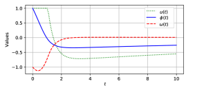
where θ=(a,b)𝜃𝑎𝑏\theta=(a,b), X=[100,100],U=[1,1]formulae-sequence𝑋100100𝑈11X=[-100,100],\,U=[-1,1] and Θ={(a,b)|a0}Θconditional-set𝑎𝑏𝑎0\Theta=\{(a,b)\,|\,a\geq 0\}. Similar problems have appeared in [Wang et al.(2015)Wang, O’Donoghue, and Boyd, Banjac and Lygeros(2019)]. The results are shown in Fig. 1, where the performance is greatly improved from initial guess of θ𝜃\theta after 2 iterations.

\subfigure

[System behavior under ADP controls with different cost function estimate.]Refer to caption \subfigure[System behavior with trained and untrained cost function from different initial states.]Refer to caption
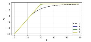
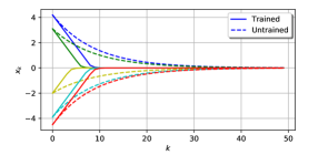
Figure 1: Closed-loop system behavior under ADP control.
Example 9.

Consider a torsional pendulum system with dynamics given as:

ϕ˙=ω,ω˙=M1(mglsinϕγω+τ),ϕ(π/2,π/2),ω[2,2],τ[1,1],formulae-sequence˙italic-ϕ𝜔formulae-sequence˙𝜔superscript𝑀1𝑚𝑔𝑙italic-ϕ𝛾𝜔𝜏formulae-sequenceitalic-ϕ𝜋2𝜋2formulae-sequence𝜔22𝜏11\dot{\phi}=\omega,\,\dot{\omega}=M^{-1}(-mgl\sin{\phi}-\gamma\omega+\tau),\,\phi\in(-\pi/2,\pi/2),\,\omega\in[-2,2],\,\tau\in[-1,1],

where m=1/3 kg𝑚13 kgm=1/3\emph{ kg}, l=3/2 m𝑙32 ml=3/2\emph{ m}, M=4/3ml2𝑀43𝑚superscript𝑙2M=4/3ml^{2}, γ=0.2𝛾0.2\gamma=0.2 and g=9.8 m/s2𝑔9.8 msuperscripts2g=9.8\emph{ m}/\emph{s}^{2}. The discrete dynamics, denoted as f()𝑓f(\cdot) and used for ADP control, is obtained by forward Euler method with sampling time 0.1 s0.1 s0.1\emph{ s} where the state is x=[ϕ,ω]T𝑥superscriptitalic-ϕ𝜔Tx=[\phi,\omega]^{\emph{T}} with T denoting transpose operation, and the control is u=τ𝑢𝜏u=\tau. Then the problem data is given as:

xk+1=f(xk,uk),H(x,u,J)=xTQx+uTRu+0.95J(f(x,u)),J~(x,θ)=xTPx+b,formulae-sequencesubscript𝑥𝑘1𝑓subscript𝑥𝑘subscript𝑢𝑘formulae-sequence𝐻𝑥𝑢𝐽superscript𝑥T𝑄𝑥superscript𝑢T𝑅𝑢0.95𝐽𝑓𝑥𝑢~𝐽𝑥𝜃superscript𝑥T𝑃𝑥𝑏x_{k+1}=f(x_{k},u_{k}),\,H(x,u,J)=x^{\emph{T}}Qx+u^{\emph{T}}Ru+0.95J(f(x,u)),\,\tilde{J}(x,\theta)=x^{\emph{T}}Px+b,

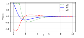
where Q𝑄Q is identity matrix, R=0.1𝑅0.1R=0.1, θ=(P,b)𝜃𝑃𝑏\theta=(P,b), X2𝑋superscript2X\subset\mathbb{R}^{2}, U=[1,1]𝑈11U=[-1,1] and Θ={(P,b)|P0}Θconditional-set𝑃𝑏succeeds-or-equals𝑃0\Theta=\{(P,b)\,|\,P\succeq 0\}. Similar example has appeared in [Si and Wang(2001), Liu and Wei(2013)]. We set S=100𝑆100S=100, K=5𝐾5K=5, pk=0.5subscript𝑝𝑘0.5p_{k}=0.5 for all k𝑘k, and λ=0.1𝜆0.1\lambda=0.1 so that the lookahead steps in average is 1/λ=101𝜆101/\lambda=10. The closed loop system behavior with initial θ𝜃\theta and θ𝜃\theta after 555 iterations are shown in Fig. 2 where the continuous system dynamics is solved by ode45. The control performance is greatly improved.

\subfigure

[With initial guess of θ𝜃\theta.]Refer to caption \subfigure[With θ𝜃\theta after 5 training iterations.]Refer to caption

Figure 2: Closed-loop system behavior under ADP control with untrained and trained θ𝜃\theta.

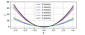
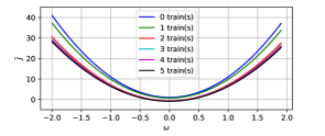
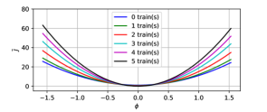
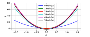
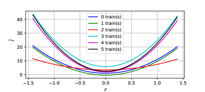
Here we show the cost function plots along the axes where ω=0𝜔0\omega=0 and ϕ=0italic-ϕ0\phi=0, and the cost estimates converged. Besides, we compared the performance of λ𝜆\lambda-PIR with approximated implementation of VI where in (5) the evaluation step is always applying TμkJ~subscript𝑇superscript𝜇𝑘~𝐽T_{\mu^{k}}\tilde{J}, and optimistic policy iteration (OPI) where the evaluation is performed as TμkJ~superscriptsubscript𝑇superscript𝜇𝑘~𝐽T_{\mu^{k}}^{\ell}\tilde{J} with \ell fixed at 1/λ=101𝜆101/\lambda=10. OPI is analyzed by [Scherrer et al.(2015)Scherrer, Ghavamzadeh, Gabillon, Lesner, and Geist] for finite state case and is known to be closed related to λ𝜆\lambda-PI. In λ𝜆\lambda-PIR, the Tμk(λ)J~superscriptsubscript𝑇superscript𝜇𝑘𝜆~𝐽T_{\mu^{k}}^{(\lambda)}\tilde{J} step occurred in the 222nd iteration, and one can observe a ‘boost’ towards the optimal in Fig. 3, while VI in Fig. 4 is yet to converge in the 555th iteration. On the other hand, although OPI in Fig. 4 behaves quite similarly to λ𝜆\lambda-PIR, it does require more sampling efforts compared to λ𝜆\lambda-PIR. The results here imply that λ𝜆\lambda-PIR combined the benefits of those two methods.

\subfigure

[Cost function along the axis ω=0𝜔0\omega=0 after different training iterations.]Refer to caption \subfigure[Cost function along the axis ϕ=0italic-ϕ0\phi=0 after different training iterations.]Refer to caption

Figure 3: Cost function estimates along the axes ϕ=0italic-ϕ0\phi=0 and ω=0𝜔0\omega=0 after different training iterations.
\subfigure

[Cost function along the axis ω=0𝜔0\omega=0 for VI.]Refer to caption \subfigure[Cost function along the axis ω=0𝜔0\omega=0 for OPI.]Refer to caption

Figure 4: Cost function estimates of VI and OPI along the axis ω=0𝜔0\omega=0.
Example 10.

Consider a nonlinear system with dynamics given as

y˙=asinz,z˙=y2+v,y[2,2],z(π/2,π/2),v[1,1],formulae-sequence˙𝑦𝑎𝑧formulae-sequence˙𝑧superscript𝑦2𝑣formulae-sequence𝑦22formulae-sequence𝑧𝜋2𝜋2𝑣11\dot{y}=a\sin{z},\,\dot{z}=-y^{2}+v,\,y\in[-2,2],\,z\in(-\pi/2,\pi/2),\,v\in[-1,1],

where a𝑎a is some constant. This is Example 13.13 in [Khalil(2001)] and the goal is to set y𝑦y to 111. By state feedback linearization method, we can obtain a controller given as

v=y2l1(y1)+l2asinzacosz𝑣superscript𝑦2subscript𝑙1𝑦1subscript𝑙2𝑎𝑧𝑎𝑧v=y^{2}-\frac{l_{1}(y-1)+l_{2}a\sin{z}}{a\cos{z}}

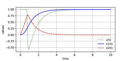
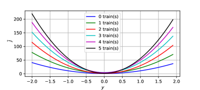
where l1subscript𝑙1l_{1} and l2subscript𝑙2l_{2} are parameters to be designed which impact the closed-loop poles. Denote x=[y1,z]T𝑥superscript𝑦1𝑧Tx=[y-1,z]^{\emph{T}} and u=v𝑢𝑣u=v, and following the same procedure and using the algorithm data as in Example 9, we can obtain a cost estimate J~(x,θ)~𝐽𝑥𝜃\tilde{J}(x,\theta). Fig. 5 shows a comparison of system behavior under state feedback linearization and under ADP control. The constant a𝑎a is set to 111 and the poles are chosen to be both at 11-1 so that the control constraint is not violated. One can see that the control response in the ADP control case is faster. The cost function estimates along axes z=0𝑧0z=0 and y=0𝑦0y=0 are shown in Fig. 3, where the cost estimates converge after 5 iterations.

\subfigure

[System behavior and control signal with state feedback linearization.]Refer to caption \subfigure[System behavior and control signal with ADP control with trained θ𝜃\theta.]Refer to caption
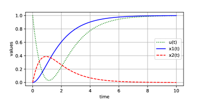
Figure 5: Closed-loop system behavior under state feedback linearization and ADP with trained θ𝜃\theta.
\subfigure

[Cost function along the axis z=0𝑧0z=0 after different training iterations.]Refer to caption \subfigure[Cost function along the axis y=0𝑦0y=0 after different training iterations.]Refer to caption

Figure 6: Cost function estimates along the axes where z=0𝑧0z=0 and y=0𝑦0y=0 after different iterations of training.

6 Conclusions

We presented results related to λ𝜆\lambda-PIR aided by abstract DP models. The λ𝜆\lambda-PIR is originally devised for finite policy problems and our results showed that the algorithm is also well-defined for contractive models with infinite states and the algorithmic convergence can be ensured for problems with infinite policies by adding an additional condition, which can be dismissed if the problem exhibits a linear structure. We exemplified a data-driven approximated implementation of the algorithm to estimate cost functions for constrained optimal control problems and the obtained estimates resulted in good closed-loop behavior when embedded in ADP for online control in numerical examples.

\acks

This work was supported by the Swedish Foundation for Strategic Research, the Swedish Research Council, and the Knut and Alice Wallenberg Foundation. The authors are grateful to Prof. Dimitri P. Bertsekas for discussions pointing to abstract DP models and to the connection between λ𝜆\lambda-PI and proximal algorithms, and for his suggestions to improve this work. The helpful comments from the reviewers are also acknowledged.

References

  • [Banjac and Lygeros(2019)] Goran Banjac and John Lygeros. A data-driven policy iteration scheme based on linear programming. In 2019 IEEE 58th Conference on Decision and Control (CDC). IEEE, 2019.
  • [Bellemare et al.(2016)Bellemare, Ostrovski, Guez, Thomas, and Munos] Marc G. Bellemare, Georg Ostrovski, Arthur Guez, Philip S. Thomas, and Rémi Munos. Increasing the action gap: New operators for reinforcement learning. In Thirtieth AAAI Conference on Artificial Intelligence, 2016.
  • [Bertsekas and Shreve(1978)] Dimitiri P. Bertsekas and Steven Shreve. Stochastic optimal control: the discrete-time case. Academic Press, 1978.
  • [Bertsekas(2012)] Dimitri P. Bertsekas. Lambda-policy iteration: A review and a new implementation. Reinforcement learning and approximate dynamic programming for feedback control, pages 381–406, 2012.
  • [Bertsekas(2018a)] Dimitri P. Bertsekas. Abstract dynamic programming. Athena Scientific, 2nd edition, 2018a.
  • [Bertsekas(2018b)] Dimitri P. Bertsekas. Proximal algorithms and temporal difference methods for solving fixed point problems. Computational Optimization and Applications, 70(3):709–736, 2018b.
  • [Bertsekas(2019)] Dimitri P. Bertsekas. Reinforcement learning and optimal control. Athena Scientific, 2019.
  • [Bertsekas and Ioffe(1996)] Dimitri P. Bertsekas and Sergey Ioffe. Temporal differences-based policy iteration and applications in neuro-dynamic programming. lab. for info. and decision systems report lids-p-2349, 1996.
  • [Bertsekas and Tsitsiklis(1996)] Dimitri P. Bertsekas and John N. Tsitsiklis. Neuro-dynamic programming, volume 5. Athena Scientific Belmont, MA, 1996.
  • [Bian and Jiang(2016)] Tao Bian and Zhong-Ping Jiang. Value iteration, adaptive dynamic programming, and optimal control of nonlinear systems. In 2016 IEEE 55th Conference on Decision and Control (CDC), pages 3375–3380. IEEE, 2016.
  • [Busoniu et al.(2017)Busoniu, Babuska, De Schutter, and Ernst] Lucian Busoniu, Robert Babuska, Bart De Schutter, and Damien Ernst. Reinforcement learning and dynamic programming using function approximators. CRC press, 2017.
  • [De Farias and Van Roy(2003)] Daniela Pucci De Farias and Benjamin Van Roy. The linear programming approach to approximate dynamic programming. Operations research, 51(6):850–865, 2003.
  • [Diamond and Boyd(2016)] Steven Diamond and Stephen Boyd. CVXPY: A Python-embedded modeling language for convex optimization. Journal of Machine Learning Research, 17(83):1–5, 2016.
  • [Khalil(2001)] Hassan K. Khalil. Nonlinear systems. Pearson, 3rd edition, 2001.
  • [Liu and Wei(2013)] Derong Liu and Qinglai Wei. Policy iteration adaptive dynamic programming algorithm for discrete-time nonlinear systems. IEEE Transactions on Neural Networks and Learning Systems, 25(3):621–634, 2013.
  • [Scherrer et al.(2015)Scherrer, Ghavamzadeh, Gabillon, Lesner, and Geist] Bruno Scherrer, Mohammad Ghavamzadeh, Victor Gabillon, Boris Lesner, and Matthieu Geist. Approximate modified policy iteration and its application to the game of Tetris. Journal of Machine Learning Research, 16:1629–1676, 2015.
  • [Si and Wang(2001)] Jennie Si and Yu-Tsung Wang. Online learning control by association and reinforcement. IEEE Transactions on Neural networks, 12(2):264–276, 2001.
  • [Sutton(1988)] Richard S. Sutton. Learning to predict by the methods of temporal differences. Machine learning, 3(1):9–44, 1988.
  • [Sutton and Barto(2018)] Richard S. Sutton and Andrew G. Barto. Reinforcement learning: An introduction. MIT press, 2018.
  • [Szepesvári(2010)] Csaba Szepesvári. Algorithms for reinforcement learning. Synthesis lectures on artificial intelligence and machine learning. Morgan & Claypool Publishers, 2010.
  • [Thiery and Scherrer(2010)] Christophe Thiery and Bruno Scherrer. Least-squares policy iteration: Bias-variance trade-off in control problems. In Proceedings of the 27th International Conference on Machine Learning (ICML-10), pages 1071–1078, Haifa, Israel, June 2010. Omnipress.
  • [Tsitsiklis and Van Roy(1997)] John N. Tsitsiklis and Benjamin Van Roy. An analysis of temporal-diffference learning with function approximation. IEEE Transactions on Automatic Control, 42(5):674–690, 1997.
  • [Wang et al.(2015)Wang, O’Donoghue, and Boyd] Yang Wang, Brendan O’Donoghue, and Stephen Boyd. Approximate dynamic programming via iterated bellman inequalities. International Journal of Robust and Nonlinear Control, 25(10):1472–1496, 2015.
  • [Watkins(1989)] Christopher John Cornish Hellaby Watkins. Learning from delayed rewards. PhD thesis, King’s College, Cambridge, 1989.
  • [Yu and Bertsekas(2012)] Huizhen Yu and Dimitri P. Bertsekas. Weighted Bellman equations and their applications in dynamic programming. laboratory for information and decision systems report lids-p-2876, 2012.
  • [Yu and Bertsekas(2015)] Huizhen Yu and Dimitri P. Bertsekas. A mixed value and policy iteration method for stochastic control with universally measurable policies. Mathematics of Operations Research, 40(4):926–968, 2015.
  • [Yu et al.(2018)Yu, Mahmood, and Sutton] Huizhen Yu, A. Rupam Mahmood, and Richard S. Sutton. On generalized Bellman equations and temporal-difference learning. Journal of Machine Learning Research, 19(1):1864–1912, 2018.