Simplified Eigenvalue Analysis for Turbomachinery Aerodynamics with Cyclic Symmetry

Abstract

Eigenvalue analysis is widely used for linear instability analysis in both external and internal aerodynamics. It typically involves finding the steady state, linearizing around it to obtain the Jacobian, and then solving for its eigenvalues and eigenvectors. When the flow is modelled with Reynolds-averaged Navier–Stokes equations with a large boundary-layer-resolving mesh, the resulting eigenvalue problem can be of very high dimensions, and is thus computationally very challenging. To reduce the computational cost, a simplified approach is proposed to compute the eigenvalues and eigenvectors, by exploiting the cyclic symmetric nature of annular fluid domain for typical compressors. It is shown that via a rotational transformation, the Jacobian can be reduced to a block circulant matrix, whose eigenvalues and eigenvectors then can be computed using only one sector of the entire domain. This simplified approach significantly lowers the memory overhead and the CPU time of the eigenvalue analysis without compromising on the accuracy. The proposed method is applied to the eigenvalue analysis of an annular compressor cascade with 22 repeated sectors and it is shown the spectrum of the whole annulus can be obtained by using the information of 1 sector only, demonstrating the effectiveness of the proposed method.

Nomenclature

$A$  =	Jacobian matrix for the whole annulus
$B$  =	circulant matrix
$b_{i}$  =	entries of a circulant matrix
$\mathbf{e},\hat{\mathbf{e}}$  =	basis vector of the original and rotated references
$\mathbf{R}$  =	residual vector
$T$  =	rotational transformation matrix
$\mathbf{U}$  =	flow field vector
$\mathbf{v},\mathbf{w}$  =	eigenvectors
$\rho_{m}$  =	$M$th complex roots of 1
$\theta$  =	pitch angle between two neighboring sectors
$\lambda$  =	eigenvalue

1 Introduction

Eigenvalue analysis based on the Reynolds-averaged Navier–Stokes (RANS) equations is a widely used approach to study the linear instability of external flow problems [1] such as the transonic shock buffet for airfoil [2, 3] and for wings [4, 5, 6]. In those works, the RANS equations are linearized about the steady state and an eigenvalue problem is solved for the resulting large sparse linear system of equations. The stability of the system is then determined by the existence of eigenvalues with positive real parts. This approach is shown to be capable of determining the stability boundary that is consistent with unsteady RANS approach, but at orders-of-magnitude lower a cost.

Eigenvalue-based linear instability analysis has also been used for turbomachinery applications, mainly regarding the flow-instability inception towards the stall boundary of compressors. A general approach to predict the onset of such instability using the eigenvalue method is proposed in [7] and has been successfully applied to both axial and centrifugal compressors [8, 9]. Different from the application on airfoil and wing aerodynamics where the flow is modelled with three-dimensional RANS equations, these works on compressor stability study use a simplified approach by modelling the effect of the blades with body forces and ignoring the circumferential variation of the flow field. With such simplification, a small eigenvalue problem can be formulated and solved in the meridional plane to predict the linear instability of the system. Although the method is shown to predict the turbomachinery flow-instability onset with plausible accuracy, ignoring the three-dimensional details naturally brings error that is not known a priori. Besides, modern compressors are designed with increasingly higher loading and exhibit strong three-dimensional effect, which needs to be accounted for when studying the flow instability [10]. Furthermore, three-dimensional RANS calculation has become routine practice for turbomachinery industry and consequently the flow-instability inception prediction needs to be based on RANS equations as well in order to retain the same modelling capability.

One key factor limiting the application of the RANS-based eigenvalue analysis to turbomachinery is its high computational cost. Although the steady state performance of compressors can be computed using a single passage mesh, which typically has grid points on the order of one million, whole annulus domain needs to be employed in order to capture the instability onset. Consequently, a computational mesh one to three orders of magnitude larger than typical airfoil/wing applications is needed, and therefore computing eigenvalue (even a small subset of it) based on RANS equations for compressors is computationally much more demanding.

Turbomachinery components usually assume cyclic symmetric shape and so is the flow field inside, and the cyclic symmetry can be exploited in order to simplify the computation. It is in fact established practice for computing the natural frequencies and vibrational mode shapes of periodic structures with cyclic structure [11]. One first meshes one sector of the entire structure and specifies the nodal diameter and the natural frequencies and mode shapes for the specifies nodal diameters can be computed. Looping over all possible nodal diameters allows one to obtain all natural frequencies and mode shapes for the entire structure. Throughout the whole process, all computations are performed based on one sector of the domain, thus requires much less computational resource and much shorter CPU time, compared to the whole-annulus computation. Such simplification approach was revisited in [12] for flow problems with translational periodicity and was successfully demonstrated on linear cascade type of problems. However, the methodology proposed therein is not directly applicable to cases with rotational periodicity, which are representative of real compressors. Therefore, it is desirable to extend the methodology to flow problems with rotational periodicity in order to significantly simplify the eigenvalue computation in order to study the whole annulus compressor flow instability.

In this work, an extension of the method proposed in [12] is developed so that it can be directly applied to the eigenvalue calculation for cyclic symmetric domains using one sector of the geometry only. In the remaining part of the paper, the theoretical basis for the simplification of the eigenvalue computation is first reviewed in Sec. 2 with particular focus on the linearized RANS equations. The application of the proposed method is then applied to the eigenvalue calculation for an annular compressor cascade case to demonstrate its effectiveness in reducing the computational cost and results are discussed in Sec. 3. Conclusions are given in Sec. 4.

2 Theoretical framework

2.1 Eigenvalue analysis of block circulant matrices

A circulant matrix $B$ has the form as follows

$$B=\left[\begin{array}[]{c c c c }b_{0}&b_{1}&\cdots&b_{M-1}\\ b_{M-1}&b_{0}&\cdots&b_{M-2}\\ \vdots&\vdots&\ddots&\vdots\\ b_{1}&b_{2}&\cdots&b_{0}\end{array}\right].$$

Due to its cyclic symmetric nature, it can be verified that matrix $B$ has the following eigenvalues and eigenvectors

$$\lambda_{m}=\sum_{k=0}^{M-1}b_{k}\rho_{m}^{k}$$

and

$$\mathbf{v}_{m}=\left[1,\rho_{m},\rho_{m}^{2},\cdots,\rho_{m}^{M-1}\right]^{T}~{}~{}(m=0,1,2,\dots,M-1),$$

where

$$\rho_{m}=\text{e}^{{~{}\text{j}}2\pi m/M}~{}~{}(m=0,1,2,\dots,M-1)$$

are the $M$th complex roots of 1, and j is the imaginary unit. It can easily be verified that all eigenvectors are orthogonal to each other, i.e.,

$$\mathbf{v}_{m_{1}}\perp\mathbf{v}_{m_{2}}~{}~{}\text{if}~{}~{}m_{1}\neq m_{2}.$$

Matrix $B$ becomes a block circulant matrix when each $b_{i}$ is an $N\times N$ square matrix. It has long been discovered that the computation of the eigenvalue and eigenvectors of a block circulant matrix can also be simplified by exploiting its cyclic symmetric nature[13]. It can be shown that all the $M\times N$ eigenvector of the block circulant matrix can be divided into $M$ groups, with each group containing $N$ vectors. The $n$th eigenvector in the $m$th group, denoted as $\mathbf{w}_{m,n}$, should be of the following form

$$\mathbf{w}_{m,n}=\left[1,\rho_{m},\rho_{m}^{2},\cdots,\rho_{m}^{M-1}\right]^{T}\mathbf{v}_{m,n}$$

where $\mathbf{v}_{m,n}$ is a vector of length $N$. In order for $\mathbf{w}_{m,n}$ to be an eigenvector, the following equation has to be satisfied

$$B\mathbf{w}_{m,n}=\lambda_{m,n}\mathbf{w}_{m,n}$$

which can be expanded as follows

$$\begin{array}[]{rcl}(b_{0}+\rho_{m}b_{1}+\cdots+\rho_{m}^{M-1}b_{M-1})\mathbf{v}_{m,n}&=&\lambda_{m,n}\mathbf{v}_{m,n}\\ (b_{M-1}+\rho_{m}b_{0}+\cdots+\rho_{m}^{M-1}b_{M-2})\mathbf{v}_{m,n}&=&\lambda_{m,n}\rho_{m}\mathbf{v}_{m,n}\\ {}\hfil&\vdots&{}\\ (b_{1}+\rho_{m}b_{2}+\cdots+\rho_{m}^{M-1}b_{0})\mathbf{v}_{m,n}&=&\lambda_{m,n}\rho_{m}^{M-1}\mathbf{v}_{m,n}.\end{array}$$

It can be verified that any two equations in the linear system above are equivalent. Therefore $\lambda_{m,n}$ and $\mathbf{v}_{m,n}$ can be found by solving the first equation only. That is, they are the $n$th eigenvalue and eigenvector of the $N\times N$ matrix $B_{m}$

$$B_{m}=b_{0}+\rho_{m}b_{1}+\rho_{m}^{2}b_{2}+\cdots+\rho_{m}^{M-1}b_{M-1}.$$

Therefore, the eigen analysis of the large matrix $B$ of dimension $MN\times MN$ can be obtained via the eigen analysis of $M$ smaller matrix $B_{m}$ of dimension $N\times N$, significantly simplifying the computation.

2.2 Jacobian matrix of the linearized RANS equations

For a typical finite volume solver based on the RANS equations, the vector $\mathbf{U}$ that satisfies

$$\mathbf{R}(\mathbf{U})=0$$

is the steady state solution. The time-dependent behavior of the flow solution is governed by the unsteady form

$$\dfrac{d\mathbf{U}}{dt}=\mathbf{R}(\mathbf{U}).$$

To study its linear stability, one could linearize the nonlinear residual vector $\mathbf{R}$ about the steady state with respect to the flow solution vector $\mathbf{U}$ to obtain the Jacobian matrix $A$

$$A:=\dfrac{\partial\mathbf{R}}{\partial\mathbf{U}}$$

and compute its eigenvalues and eigenvectors.

To facilitate the discussion, it is assumed that the computational mesh is cyclic symmetric with $M$-periodicity. Consequently, the full-annulus mesh can be divided into $M$ non-overlapping zones, each of which containing $N$ grid points, as illustrated in Fig. 1. In addition, the grid points in each zone is arranged in such a way that the $n$th point in zone $m_{1}$ is the $n$th point in zone $m_{2}$ rotated by an angle of $2(m_{2}-m_{1})\pi/M$.

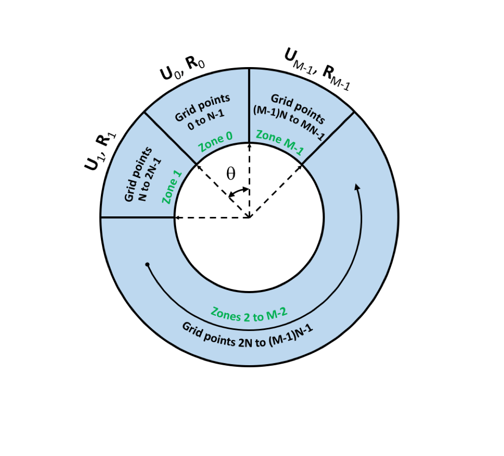
Figure 1: Arrangement of the computational meshes in the cyclic symmetric circular domain.

Due to the cyclic symmetry of the mesh, the Jacobian matrix $A$ can be partitioned as a block matrix as follows

$$A=\left[\begin{array}[]{cccc}\dfrac{\partial\mathbf{R}_{0}}{\partial\mathbf{U}_{0}}&\dfrac{\partial\mathbf{R}_{0}}{\partial\mathbf{U}_{1}}&\dots&\dfrac{\partial\mathbf{R}_{0}}{\partial\mathbf{U}_{M-1}}\\ \dfrac{\partial\mathbf{R}_{1}}{\partial\mathbf{U}_{0}}&\dfrac{\partial\mathbf{R}_{1}}{\partial\mathbf{U}_{1}}&\dots&\dfrac{\partial\mathbf{R}_{1}}{\partial\mathbf{U}_{M-1}}\\ \vdots&\vdots&\ddots&\vdots\\ \dfrac{\partial\mathbf{R}_{M-1}}{\partial\mathbf{U}_{0}}&\dfrac{\partial\mathbf{R}_{M-1}}{\partial\mathbf{U}_{1}}&\dots&\dfrac{\partial\mathbf{R}_{M-1}}{\partial\mathbf{U}_{M-1}}\end{array}\right]$$

where $\mathbf{U}_{m}$ and $\mathbf{R}_{m}$ are the vectors of the flow variables and the nonlinear residual for the grid points in the $m$th zone, each being a vector of length $5N$ for Euler/laminar or $6N$ for turbulent flow with a one-equation turbulence model, and each block $\dfrac{\partial\mathbf{R}_{[\cdot]}}{\partial\mathbf{U}_{[\cdot]}}$ is a $5N\times 5N$ or $6N\times 6N$ matrix.

Note that block matrices $\dfrac{\partial\mathbf{R}_{[\cdot]}}{\partial\mathbf{U}_{[\cdot]}}$ are second-order tensors that are invariant to the coordinate system used, and can be expressed using tensor product as

$$\dfrac{\partial\mathbf{R}_{m_{1}}}{\partial\mathbf{U}_{m_{2}}}=\left[M_{m_{1},m_{2}}\right]_{i,j}\mathbf{e}_{i}\mathbf{e}_{j}=\left[\hat{M}_{m_{1},m_{2}}\right]_{i,j}\hat{\mathbf{e}}_{i}\hat{\mathbf{e}}_{j}$$ (1)

where $\{\mathbf{e}_{1},\mathbf{e}_{2},\mathbf{e}_{3}\}$ are the basis vectors in the coordinate frame fixed to the computational mesh and $\mathbf{e}_{i}\mathbf{e}_{j}$ is short for the tensor product $\mathbf{e}_{i}\otimes\mathbf{e}_{j}$. $M_{m_{1},m_{2}}$ and $\hat{M}_{m_{1},m_{2}}$ are the matrix representation of the second-order tensor $\dfrac{\partial\mathbf{R}_{m_{1}}}{\partial\mathbf{U}_{m_{2}}}$ in the coordinate systems $\{\mathbf{e}_{1},\mathbf{e}_{2},\mathbf{e}_{3}\}$ and $\{\hat{\mathbf{e}}_{1},\hat{\mathbf{e}}_{2},\hat{\mathbf{e}}_{3}\}$ respectively. Let $\{\hat{\mathbf{e}}_{1},\hat{\mathbf{e}}_{2},\hat{\mathbf{e}}_{3}\}$ be a coordinate system that is obtained by rotating $\{\mathbf{e}_{1},\mathbf{e}_{2},\mathbf{e}_{3}\}$ by $m_{1}\theta=2m_{1}\pi/M$, as shown in Fig. 2

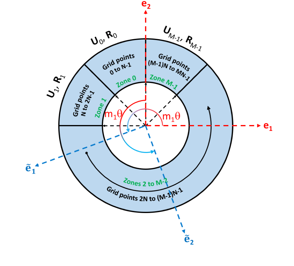
Figure 2: Arrangement of the computational meshes in the cyclic symmetric circular domain.

The basis vectors of the two coordinate systems can linked via the transformation matrix $T^{m_{1}}$ via

$$\mathbf{e}_{i}[T^{m_{1}}]_{i,j}=\hat{\mathbf{e}}_{j},$$

where the matrix $T$ denotes the rotational transform of $\theta=2\pi/M$. Substitute the $\hat{\mathbf{e}}_{i}$ in Eq. (1) yields

$$M_{m_{1},m_{2}}=T^{m_{1}}\hat{M}_{m_{1},m_{2}}T^{-m_{1}}.$$

In addition, it is straightforward to see that $\dfrac{\partial\mathbf{R}_{0}}{\partial\mathbf{U}_{m_{2}-m_{1}}}$ viewed in $\{\mathbf{e}_{1},\mathbf{e}_{2},\mathbf{e}_{3}\}$ is identical to $\dfrac{\partial\mathbf{R}_{m_{1}}}{\partial\mathbf{U}_{m_{2}}}$ viewed in $\{\tilde{\mathbf{e}}_{1},\tilde{\mathbf{e}}_{2},\tilde{\mathbf{e}}_{3}\}$. This means the matrix representation of the former in $\{\mathbf{e}_{1},\mathbf{e}_{2},\mathbf{e}_{3}\}$ is that of the latter in $\{\tilde{\mathbf{e}}_{1},\tilde{\mathbf{e}}_{2},\tilde{\mathbf{e}}_{3}\}$, i.e.,

$$\hat{M}_{m_{1},m_{2}}=M_{0,m_{2}-m_{1}}$$

and hence

$$M_{m_{1},m_{2}}=T^{m_{1}}M_{0,m_{2}-m_{1}}T^{-m_{1}}.$$

or equivalently,

$$\dfrac{\partial\mathbf{R}_{m_{1}}}{\partial\mathbf{U}_{m_{2}}}=T^{m_{1}}\dfrac{\partial\mathbf{R}_{0}}{\partial\mathbf{U}_{m_{2}-m_{1}}}T^{-m_{1}}.$$

The Jacobian matrix $A$ becomes

$$A=\left[\begin{array}[]{cccc}\dfrac{\partial\mathbf{R}_{0}}{\partial\mathbf{U}_{0}}&\dfrac{\partial\mathbf{R}_{0}}{\partial\mathbf{U}_{1}}&\dots&\dfrac{\partial\mathbf{R}_{0}}{\partial\mathbf{U}_{M-1}}\\ T\dfrac{\partial\mathbf{R}_{0}}{\partial\mathbf{U}_{M-1}}T^{-1}&T\dfrac{\partial\mathbf{R}_{0}}{\partial\mathbf{U}_{0}}T^{-1}&\dots&T\dfrac{\partial\mathbf{R}_{0}}{\partial\mathbf{U}_{M-2}}T^{-1}\\ \vdots&\vdots&\ddots&\vdots\\ T^{M-1}\dfrac{\partial\mathbf{R}_{0}}{\partial\mathbf{U}_{1}}\textasciicaron^{-(M-1)}&T^{M-1}\dfrac{\partial\mathbf{R}_{0}}{\partial\mathbf{U}_{M-2}}T^{-(M-1)}&\dots&T^{M-1}\dfrac{\partial\mathbf{R}_{0}}{\partial\mathbf{U}_{0}}T^{-(M-1)}\end{array}\right]$$

Further more, change of variable is used for $\mathbf{U}_{m}$

$$\tilde{\mathbf{U}}_{m}=T^{-m}\mathbf{U}_{m}$$

so that

$$\dfrac{\partial\mathbf{R}_{0}}{\partial\mathbf{U}_{m}}=\dfrac{\partial\mathbf{R}_{0}}{\partial\tilde{\mathbf{U}}_{m}}T^{-m}$$

The Jacobian matrix $A$ can be further rewritten to be

$$A =\left[\begin{array}[]{cccc}\dfrac{\partial\mathbf{R}_{0}}{\partial\tilde{\mathbf{U}}_{0}}&\dfrac{\partial\mathbf{R}_{0}}{\partial\tilde{\mathbf{U}}_{1}}T^{-1}&\dots&\dfrac{\partial\mathbf{R}_{0}}{\partial\tilde{\mathbf{U}}_{M-1}}T^{-(M-1)}\\ T\dfrac{\partial\mathbf{R}_{0}}{\partial\tilde{\mathbf{U}}_{M-1}}&T\dfrac{\partial\mathbf{R}_{0}}{\partial\tilde{\mathbf{U}}_{0}}T^{-1}&\dots&T\dfrac{\partial\mathbf{R}_{0}}{\partial\tilde{\mathbf{U}}_{M-2}}T^{-(M-1)}\\ \vdots&\vdots&\ddots&\vdots\\ T^{M-1}\dfrac{\partial\mathbf{R}_{0}}{\partial\tilde{\mathbf{U}}_{1}}&T^{M-1}\dfrac{\partial\mathbf{R}_{0}}{\partial\tilde{\mathbf{U}}_{M-2}}T^{-1}&\dots&T^{M-1}\dfrac{\partial\mathbf{R}_{0}}{\partial\tilde{\mathbf{U}}_{0}}T^{-(M-1)}\end{array}\right]={\mathcal{T}}B{\mathcal{T}}^{-1}$$

with matrices $\mathcal{T}$ and $B$ defined as

$$\mathcal{T}=\left[\begin{array}[]{cccc}I&0&\cdots&0\\ 0&T&\cdots&0\\ \vdots&\vdots&\dots&\vdots\\ 0&0&\cdots&T^{M-1}\end{array}\right],~{}~{}B=\left[\begin{array}[]{cccc}\dfrac{\partial\mathbf{R}_{0}}{\partial\tilde{\mathbf{U}}_{0}}&\dfrac{\partial\mathbf{R}_{0}}{\partial\tilde{\mathbf{U}}_{1}}&\dots&\dfrac{\partial\mathbf{R}_{0}}{\partial\tilde{\mathbf{U}}_{M-1}}\\ \dfrac{\partial\mathbf{R}_{0}}{\partial\tilde{\mathbf{U}}_{M-1}}&\dfrac{\partial\mathbf{R}_{0}}{\partial\tilde{\mathbf{U}}_{0}}&\dots&\dfrac{\partial\mathbf{R}_{0}}{\partial\tilde{\mathbf{U}}_{M-2}}\\ \vdots&\vdots&\ddots&\vdots\\ \dfrac{\partial\mathbf{R}_{0}}{\partial\tilde{\mathbf{U}}_{1}}&\dfrac{\partial\mathbf{R}_{0}}{\partial\tilde{\mathbf{U}}_{M-2}}&\dots&\dfrac{\partial\mathbf{R}_{0}}{\partial\tilde{\mathbf{U}}_{0}}\end{array}\right]$$

Therefore, the Jacobian matrix $A$ is similar to a block-circulant matrix $B$ and thus they have the same eigenvalues. To compute the eigenvalues and eigenvectors of the matrix $B$, we first compute $\lambda_{m,n}$ and $\mathbf{v}_{m,n}$, $n$th eigenvalue and eigenvector of the $N\times N$ matrix $B_{m}$

$$B_{m}=\dfrac{\partial\mathbf{R}_{0}}{\partial\tilde{\mathbf{U}}_{0}}+\rho_{m}\dfrac{\partial\mathbf{R}_{0}}{\partial\tilde{\mathbf{U}}_{1}}+\rho_{m}^{2}\dfrac{\partial\mathbf{R}_{0}}{\partial\tilde{\mathbf{U}}_{2}}+\cdots+\rho_{m}^{M-1}\dfrac{\partial\mathbf{R}_{0}}{\partial\tilde{\mathbf{U}}_{M-1}},$$

and the eigenvectors of $B$, $\mathbf{w}_{m,n}$, can be computed as

$$\mathbf{w}_{m,n}=\left[1,\rho_{m},\rho_{m}^{2},\cdots,\rho_{m}^{M-1}\right]^{T}\mathbf{v}_{m,n}.$$

Finally, the eigenvectors of the Jacobian matrix $A$ are $\mathcal{T}\mathbf{w}_{m,n}$, which can be calculated as follows

$$\mathcal{T}\mathbf{w}_{m,n}=\left[1,\rho_{m}T,\rho_{m}^{2}T^{2},\cdots,\rho_{m}^{M-1}T^{M-1}\right]^{T}\mathbf{v}_{m,n}.$$

It can be seen that for any of the $M$ eigenvectors of $B_{m}$, $\mathbf{v}_{m,n}(m=0,1,2,\dots,M-1)$, the corresponding $M$ eigenvectors of $A$, $\mathcal{T}\mathbf{w}_{m,n}(m=0,1,2,\dots,M-1)$ are modes with different nodal diameters. Same as for the circulant block matrix, to compute the eigenvalues and eigenvectors of the Jacobian matrix $A$, one only needs to solve the eigenvalue problem of dimension $N\times N$, significantly reducing the computational cost, especially for large CFD analysis.

3 Results

The test case used to demonstrate the usefulness of the proposed method is an annulus compressor cascade case. The cascade is produced by taking the surface of revolution at the 50% height of the NASA Rotor 67 [14]. The three-dimensional mesh has one cell in the radial direction and the subsequent analysis is thus a quasi-3D one. The compressor cascade rotates at 16,043 Revolutions per minute. The annular cascade has 22 passages in total. The mesh for the whole annulus is produced by meshing a single passage first and then copying the mesh to the whole annulus. The mesh for the entire domain has 126,808 grid points, with an average of 5,764 per zone.

3.0.1 Steady state calculation

The turbomachinery nonlinear flow solver NutsCFD is used to compute the performance of the cascade. The speedline, computed by gradually raising the back pressure until the steady state can no long converge, is shown in Fig. 3. The fully-converged steady state flow solution corresponding to the condition marked in red in Fig. 3 (to be called condition ‘A’ in the remainder of the paper) is visualized in Fig. 4, where the shock/boundary layer interaction can clearly be seen. All steady state calculations are performed using a single passage. The visualized flow fields are produced by copying the solution in the single passage to the whole annulus.

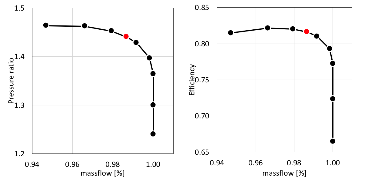
Figure 3: Total pressure ratio and isentropic efficiency of the cascade with the red circle denoting the condition for which eigenvalue analysis is performed.

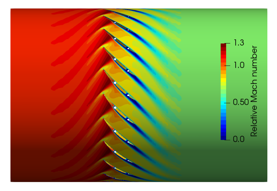
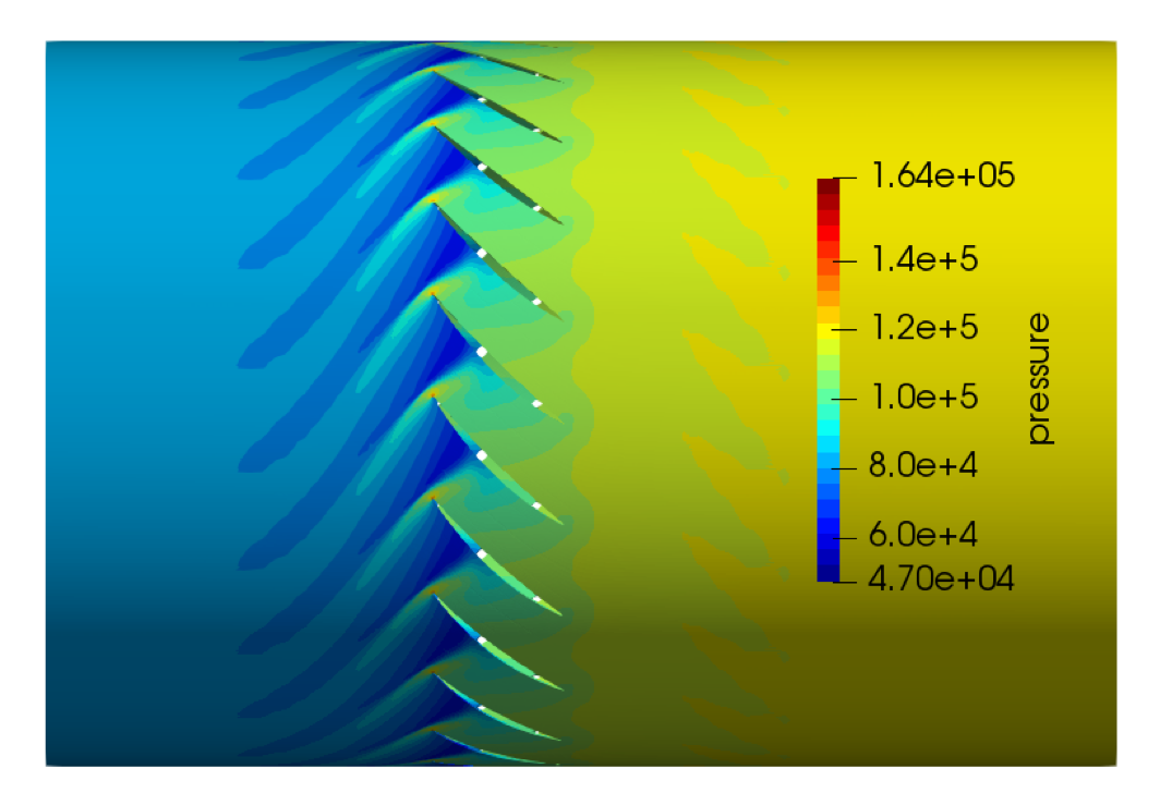
Figure 4: Contour plots for the relative Mach number (left) and pressure (right) for the converged steady state solution for condition ‘A’.

3.0.2 Eigenvalue analysis

To perform the eigenvalue analysis for condition ‘A’, we first compute the Jacobian matrix for the single passage $\dfrac{\partial\mathbf{R}_{0}}{\partial\tilde{\mathbf{U}}_{0}}$ and then exploiting the periodic boundary condition in the steady solver to obtain $\dfrac{\partial\mathbf{R}_{0}}{\partial\tilde{\mathbf{U}}_{1}}$ and $\dfrac{\partial\mathbf{R}_{0}}{\partial\tilde{\mathbf{U}}_{M-1}}$. Note that for RANS flow solver, $\dfrac{\partial\mathbf{R}_{0}}{\partial\tilde{\mathbf{U}}_{m}},(m=2,3,\dots,M-2)$ are all zeros, so $B_{m}$ can be simplified as

$$B_{m}=\dfrac{\partial\mathbf{R}_{0}}{\partial\tilde{\mathbf{U}}_{0}}+\rho_{m}\dfrac{\partial\mathbf{R}_{0}}{\partial\tilde{\mathbf{U}}_{1}}+\rho_{m}^{M-1}\dfrac{\partial\mathbf{R}_{0}}{\partial\tilde{\mathbf{U}}_{M-1}}.$$ (2)

It is well known both numerically and experimentally that the least stable modes when instability appears in rotating flows, the characteristic frequency of the instability is close to the rotating frequency, which is $\dfrac{2\pi\times 16,043}{60}=1680Hz$ for the test case used. Consequently, the matrix $B_{m}$ is scaled by $1/1680$ so that the imaginary part of the eigenvalue is equivalent to the frequency of the corresponding eigenmode expressed in terms of engine order (EO). Since the Jacobian matrix is of moderate size (of dimension $34,584\times 34,584$, and with nearly $3.7$ million non-zero entries), the sparse matrix eigenvalue solver, “eigs”, in SciPy [15] is use on a single-processor computer. The “eigs” function in SciPy is a wrapper to the widely used eigenvalue solver library ARPACK [16].

Two different methods (listed in Tab. 2) are used to compute the eigenvalues near the imaginary axis. Method 1 computes the eigenvalues of the Jacobian matrix for the whole annulus of 22 sectors, $A$. We apply complex shifts of $\sigma=i,2i$ and $3i$ and 30 interior eigenvalues are computed for each shift. A total of 90 eigenvalues can computed and they are shown in Fig. 5 as red crosses.

Method 2 computes the eigenvalues using 1 sector only. Nevertheless, it admits eigenvalues for the whole annular domain by setting $\rho_{m}$ in Eq. (2) to $\rho_{m}=\text{e}^{{~{}\text{j}}2\pi m/M}~{}~{}(m=0,1,2,\dots,M-1)$. Same as method 1, interior eigenvalues are computed using three different shifts for each $\rho_{m}$. For each shift, 2 eigenvalues are computed, resulting in a total of 132 eigenvalues (some of them appear more than once for different shifts). All eigenvalues computed using method 2 are also plotted in Fig. 5 as blue dots. If can be seen that the least stable eigenvalues (closest to the imaginary axis) are located around $(0,1)$ and a zoomed view of the eigenvalues in the nearly region is shown on the right side in Fig. 5. It can be seen that both methods can capture a relevant subset of the eigenvalues and are both sufficient in order to study the linear stability of the underlying flow problem. However, method 2 is based only on one sector of the whole annulus domain, and thus has a significantly lower memory overhead and also costs much less CPU time than method 1.

Another advantage of method 1, besides the lower computational cost, is that each eigenvalue/eigenvector computed has a known nodal diameter, which is solely determined by the $m$ value it is computed with. The nodal diameter information reveals the circumferential spatial periodicity of each particular eigenmode.

Table 2: Two methods for computing the spectrum.

method	number of sectors	matrix dimension	$\theta$ value
1	22	$760,848\times 760,848$	no need to specify
2	1	$34,584\times 34,584$	${2m\pi}/{M}~{}(m=0,1,2,\dots,M-1)$

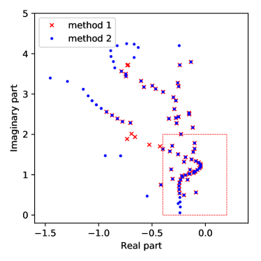
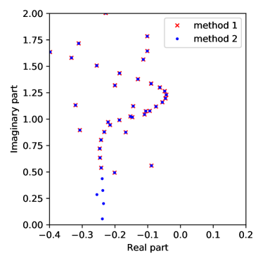
Figure 5: Computed spectrum near the imaginary axis for conditions ‘A’. Red cross: eigenvalues computed with method 1 using 22 sectors; blue dot: eigenvalues computed with method 2 using 1 sector only. A zoomed view of the eigenvalues in the region in the red box is shown on the right.

4 Conclusions

A method to simplify the eigenvalue analysis for flow problems in circular cyclic symmetric domains are proposed. The method first transform the Jacobian matrix for the whole annulus into a block circulant matrices, and subsequently reduces the eigenvalue problem of the whole circular domain to one sector only. This reduces the size of the original eigenvalue problem by a factor of $M$, $M$ being the number of passages/blades. The proposed method is applied to the eigenvalue analysis for an annular compressor cascade with $22$ sectors, and it is shown that by using $1$ sector only, spectrum of the whole domain can be obtained at a much lower memory as well as CPU time cost, demonstrating the advantage of the proposed method. Future work will explore the application of the method to realistic three-dimensional compressors to study the flow instability problems. In addition, the eigenvectors obtained can be used to construct reduced-order models for parametric study and optimization for rotating-flow instability.

References

- Theofilis [2011] Theofilis, V., “Global linear instability,” Annual Review of Fluid Mechanics, Vol. 43, 2011, pp. 319–352.
- Crouch et al. [2007] Crouch, J. D., Garbaruk, A., and Magidov, D., “Predicting the onset of flow unsteadiness based on global instability,” Journal of Computational Physics, Vol. 224, No. 2, 2007, pp. 924–940.
- Crouch et al. [2009] Crouch, J., Garbaruk, A., Magidov, D., and Travin, A., “Origin of transonic buffet on aerofoils,” Journal of Fluid Mechanics, Vol. 628, No. 628, 2009, pp. 357–369.
- Timme [2018] Timme, S., “Global instability of wing shock buffet,” ArXiv e-prints, arXiv: 1806.07299, 2018.
- Paladini et al. [2019] Paladini, E., Beneddine, S., Dandois, J., Sipp, D., and Robinet, J.-C., “Transonic buffet instability: From two-dimensional airfoils to three-dimensional swept wings,” Physical Review Fluids, Vol. 4, No. 10, 2019, p. 103906.
- Crouch et al. [2019] Crouch, J., Garbaruk, A., and Strelets, M., “Global instability in the onset of transonic-wing buffet,” Journal of Fluid Mechanics, Vol. 881, 2019, pp. 3–22.
- Sun et al. [2013] Sun, X., Liu, X., Hou, R., and Sun, D., “A General Theory of Flow-Instability Inception in Turbomachinery,” AIAA Journal, Vol. 51, No. 7, 2013, pp. 1675–1687.
- Liu et al. [2014] Liu, X., Sun, D., and Sun, X., “Basic studies of flow-instability inception in axial compressors using eigenvalue method,” Journal of Fluids Engineering, Vol. 136, No. 3, 2014, p. 031102.
- Sun et al. [2016] Sun, X., Ma, Y., Liu, X., and Sun, D., “Flow stability model of centrifugal compressors based on eigenvalue approach,” AIAA Journal, 2016, pp. 2361–2376.
- Pullan et al. [2015] Pullan, G., Young, A., Day, I., Greitzer, E., and Spakovszky, Z., “Origins and structure of spike-type rotating stall,” Journal of Turbomachinery, Vol. 137, No. 5, 2015, p. 051007.
- Thomas [1979] Thomas, D., “Dynamics of rotationally periodic structures,” International Journal for Numerical Methods in Engineering, Vol. 14, No. 1, 1979, pp. 81–102.
- Schmid et al. [2017] Schmid, P. J., Pando, M. F. D., and Peake, N., “Stability analysis for -periodic arrays of fluid systems,” Physical Review Fluids, Vol. 2, No. 11, 2017, p. 113902.
- Friedman [1961] Friedman, B., “Eigenvalues of composite matrices,” Mathematical Proceedings of the Cambridge Philosophical Society, Vol. 57, No. 1, 1961, pp. 37–49.
- Strazisar et al. [1989] Strazisar, A. J., Wood, J. R., Hathaway, M. D., and Suder, K. L., “Laser anemometer measurements in a transonic axial-flow fan rotor,” 1989.
- Jones et al. [2001] Jones, E., Oliphant, T., Peterson, P., et al., “SciPy: Open source scientific tools for Python,” 2001.
- Lehoucq et al. [1998] Lehoucq, R. B., Sorensen, D. C., and Yang, C., ARPACK users’ guide: solution of large-scale eigenvalue problems with implicitly restarted Arnoldi methods, Vol. 6, SIAM, 1998.