Influential spreaders for recurrent epidemics on networks

Abstract

The identification of which nodes are optimal seeds for spreading processes on a network is a non-trivial problem that has attracted much interest recently. While activity has mostly focused on non-recurrent type of dynamics, here we consider the problem for the Susceptible-Infected-Susceptible (SIS) spreading model, where an outbreak seeded in one node can originate an infinite activity avalanche. We apply the theoretical framework for avalanches on networks proposed by Larremore et al. [Phys. Rev. E 85, 066131 (2012)], to obtain detailed quantitative predictions for the spreading influence of individual nodes (in terms of avalanche duration and avalanche size) both above and below the epidemic threshold. When the approach is complemented with an annealed network approximation, we obtain fully analytical expressions for the observables of interest close to the transition, highlighting the role of degree centrality. Comparison of these results with numerical simulations performed on synthetic networks with power-law degree distribution reveals in general a good agreement in the subcritical regime, leaving thus some questions open for further investigation relative to the supercritical region.

I Introduction

Some epidemic outbreaks die out very rapidly, affecting just a few individuals, while others, caused by the same pathogen, survive for much longer times, infecting considerably larger fractions of the overall population Lehmann and Ahn (2018). A meme posted by a celebrity on a social network is rapidly spread to millions of users, while a similar meme posted by a less connected individual rarely becomes viral. What decides the fate of a single spreading process? One of the most important factors is where, in the connectivity pattern mediating the spreading process, the initial seed is located. Intuitively, an infection seeded in a highly connected node has a higher chance of reaching a large number of individuals, but other, less local network features may in principle play a role: For example, a node sitting at the boundary between two communities can be highly effective in giving rise to large outbreaks even if having only a few direct connections. The non-trivial question of how to identify “influential spreaders” in a network has been the focus of an impressive amount of work Pei et al. (2014); Lu et al. (2016) in the last decade. In a nutshell, the problem is the prediction of how large is, on average, a spreading event started by a single node in the network. A slightly more limited goal is to rank network nodes depending on their spreading capability and to correlate such a ranking with purely topological node features, such as degree or other types of centrality.

The seminal paper by Kitsak et al. Kitsak et al. (2010) posed in a clear manner the question, highlighting its non-triviality and reporting a strong correlation between the average size of an outbreak seeded in node $n$ and a particular type of centrality measure, the $K$-core index Seidman (1983). A huge number of other centralities have been proposed and tested as ways to identify influential spreaders Lu et al. (2016); Chen et al. (2012); Li et al. (2014), with different levels of success, depending in many cases on the type of network substrate considered for the empirical validation. Among the most firmly grounded results, Ref. Radicchi and Castellano (2016) exploited a mapping to bond percolation to relate spreading influence at the epidemic transition to nonbacktracking centrality Hashimoto (1989); Krzakala and Moore (2013), while Ref. Min (2018) extended the approach presenting a message-passing framework allowing to compute the average outbreak size for any value of the control parameter.

All these results were found for the Susceptible-Infected-Removed (SIR) dynamics Pastor-Satorras et al. (2015), the simplest model for epidemics allowing permanent immunity, or simple variants of it. For this type of models the definition of spreading influence is straightforward: Throughout the whole phase-space, outbreaks have a finite duration and the average size of an outbreak seeded in a node is the measure of how influential the node is. The other large class of epidemic models, whose simplest example is the Susceptible-Infected-Susceptible (SIS) model, describes recurrent dynamics, where each node can be reinfected over and over again Pastor-Satorras et al. (2015). While some results are available Liu and Van Mieghem (2017); Holme and Tupikina (2018), this class has received nevertheless much less attention. Our purpose in this paper is to fill this gap, performing a systematic study of the problem of identifying influential spreaders for a parallel, discrete-time, version of SIS dynamics. As for non-recurrent (SIR-like) epidemic models, the phase diagram for SIS dynamics consists in a healthy phase for small values of the control parameter (see below) separated from an epidemic phase by a critical value of the control parameter, the epidemic threshold. While the nature of the healthy phase is the same for both classes of models, the possibility of multiple reinfections changes the nature of the epidemic phase. Above the threshold there is a nonvanishing chance that a stationary “endemic” state is reached, where the epidemic survives forever, with a steady finite density of infected nodes. This possibility implies that for SIS dynamics there are different possible definitions of what an influential spreader is. Below the critical point, since all avalanches eventually end, one can take as a measure of spreading influence of node $n$ the total duration or the total size of an avalanche seeded in $n$, just as in the SIR case. In the supercritical region instead, some avalanches are infinite, i.e. they give rise to the neverending (at least in the thermodynamic limit) endemic state. In this case being an influential spreader may have two distinct meanings. Good spreaders can be nodes giving rise to an infinite avalanche with large probability or nodes giving rise to large or long finite avalanches. These definitions of influential spreaders do not necessarily coincide. For this reason we consider three main observables of interest Larremore et al. (2012):

• The probability $b_{n}$ that an avalanche seeded in node $n$ is finite (i.e., it does not lead to the endemic state above the transition). Below the transition, $b_{n}=1$; above it, $b_{n}<1$.

• The average duration $T_{n}$ of (finite) avalanches seeded in node $n$. In the following we will consider a discrete-time dynamics, hence the duration of each avalanche will be an integer.

• The average size $S_{n}$ of (finite) avalanches seeded in node $n$. This quantity is equal to the total number of activation events. Since each node can be activated more than once, $S$ can in principle be larger than the total number of nodes $N$.

Another observable of interest is the coverage, the average number of distinct nodes reached by an avalanche Boguñá et al. (2013). We performed some comparisons between this quantity and $S_{n}$, finding minimal differences. For this reason we will not consider the coverage in the following.

II Theoretical approach

II.1 Quenched Mean-Field theory

The identification of influential spreaders for SIS dynamics is greatly helped by the application of the general quenched mean-field (QMF) Wang et al. (2003); Van Mieghem et al. (2009); Gómez et al. (2010); Castellano and Pastor-Satorras (2010) theoretical approach for avalanches on networks proposed by Larremore et al. in Ref. Larremore et al. (2012). In that paper a comprehensive theory is presented for the statistical properties of avalanches when the dynamical process is determined by a matrix $A_{nm}$, whose individual entry is the probability that the avalanche propagates from node $n$ to node $m$. The approach predicts a transition between a subcritical regime with all avalanches finite ($b_{n}=1$) and a supercritical regime where a fraction $1-b_{n}$ of all avalanches lasts forever. The transition depends on the largest eigenvalue $\lambda$ of the $A$ matrix. If $\lambda<\lambda_{c}^{QMF}=1$ the system is subcritical, if $\lambda>\lambda_{c}^{QMF}$ the system is supercritical and infinite avalanches start to appear.

We can apply this theory to the SIS dynamics by considering a parallel discrete-time version of it, analogous to the Independent Cascade Model (ICM) version of SIR dynamics Goldenberg et al. (2001). In this dynamics, at each time step each infected node attempts to transmit the infection to all its direct neighbors and each independent attempt succeeds with probability $p$. After attempting to infect all its neighbors an infected node recovers and switches back to the susceptible state with a recovery time fixed to 1. The probability that an avalanche propagates from node $n$ to $m$ is therefore $A_{nm}=pa_{nm}$, where $a_{nm}$ is the unweighted adjacency matrix of the network. Clearly, the largest eigenvalue of $A$ is $\lambda=p\Lambda_{M}$, where $\Lambda_{M}$ is the largest eigenvalue of the adjacency matrix $a$. As a consequence the epidemic threshold is $p_{c}^{QMF}=1/\Lambda_{M}$.

II.1.1 Probability of observing a finite avalanche

Within QMF theory the probability $b_{n}$ of having a finite avalanche is obtained by solving iteratively the equation

$$b_{n} = \prod_{m=1}^{N}[(1-A_{nm})+A_{nm}b_{m}]$$ (1)

$$= \prod_{m=1}^{N}[1-pa_{nm}(1-b_{m})].$$

As shown in Ref. Larremore et al. (2012) this equation admits a solution $b_{n}=1$ for any $\lambda$ and for $\lambda>1$, i.e. in the supercritical regime, another stable solution $b_{n}<1$.

II.1.2 Average avalanche duration

Let us consider $c_{n}(t)$ as the probability that an avalanche has a duration smaller than or equal to $t$, with $c_{n}(0)=0$, by definition. The probability $c_{n}(t)$ fulfills the recurrence equation Larremore et al. (2012)

$$c_{n}(t+1)=\prod_{m=1}^{N}\left[(1-A_{nm})+A_{nm}c_{m}(t)\right].$$ (2)

In the limit $t\to\infty$, $c_{n}(t)\to b_{n}$, where $b_{n}=1$ in the subcritical phase, and $b_{n}<1$ in the supercritical phase; hence Eq. (1). Consider $c_{n}(t)=b_{n}-f_{n}(t)$, with $f_{n}(0)=b_{n}$. For sufficiently large $t$, $f_{n}(t)$ is small, so that we can linearize Eq. (2) to obtain Larremore et al. (2012)

$$f_{n}(t)=\sum_{m}D_{nm}f_{m}(t-1),$$ (3)

where for the SIS process

$$D_{nm}=\frac{A_{nm}b_{n}}{(1-A_{nm})+A_{nm}b_{m}}=\frac{pb_{n}a_{nm}}{1-p+pb_{m}},$$ (4)

that, in the subcritical phase, where $b_{n}=1$, reduces to $D_{nm}=A_{nm}=pa_{nm}$. The avalanche duration distribution $p_{n}(t)$ is given by

$$p_{n}(t)=c_{n}(t)-c_{n}(t-1)=f_{n}(t-1)-f_{n}(t).$$ (5)

Therefore, we can write the average avalanche duration $T_{n}$ as

$$T_{n} = \sum_{t=1}^{\infty}tp_{n}(t)=\sum_{t=1}^{\infty}tf_{n}(t-1)-\sum_{t=1}^{\infty}tf_{n}(t)$$ (6)

$$= f_{n}(0)+\sum_{t=2}^{\infty}tf_{n}(t-1)-\sum_{t=1}^{\infty}tf_{n}(t)$$

$$= b_{n}+\sum_{t=1}^{\infty}(t+1)f_{n}(t)-\sum_{t=1}^{\infty}tf_{n}(t)$$

$$= b_{n}+\sum_{t=1}^{\infty}f_{n}(t)\equiv b_{n}+R_{n}.$$

If $f_{n}(t)$ decreases sufficiently fast, we can assume that the linearization of $f_{n}(t)$ is valid for all times $t$, to obtain

$$R_{n} = \sum_{t=1}^{\infty}f_{n}(t)=\sum_{m}D_{nm}\sum_{t=1}^{\infty}f_{m}(t-1)$$ (7)

$$= \sum_{m}D_{nm}\left[f_{m}(0)+\sum_{t=1}^{\infty}f_{m}(t)\right]$$

$$= \sum_{m}D_{nm}\left[b_{m}+R_{m}\right].$$

Combining the previous equations, we have

$$T_{n}=b_{n}+\sum_{m}D_{nm}T_{m}.$$ (8)

We can obtain an exact expression at the QMF level by inverting this linear relationship, obtaining

$$T=[I-D]^{-1}B,$$ (9)

where $T=(T_{1},\ldots,T_{N})^{T}$, $B=(b_{1},\ldots,b_{N})^{T}$, and $I$ is the identity matrix.

II.1.3 Average avalanche size

From Ref. Larremore et al. (2012), the generating function of the avalanche size distribution $p_{n}(s)$,

$$\phi_{n}(z)=\sum_{s}e^{-sz}p_{n}(s),$$ (10)

fulfills the equation

$$\phi_{n}(z)=e^{-z}\prod_{m}[1+\sum_{m}(\phi_{m}(z)-1)H_{nm}],$$ (11)

where

$$H_{nm}=\frac{b_{m}pa_{nm}}{1-p+b_{m}p}$$ (12)

in the SIS process. Taking logarithms of both sides of Eq. (11), deriving with respect to $z$ and setting $z=0$ one obtains

$$\frac{\phi_{n}^{\prime}(0)}{\phi_{n}(0)}=-1+\sum_{m}\frac{H_{nm}\phi_{m}^{\prime}(0)}{1+(\phi_{m}(0)-1)H_{nm}}.$$ (13)

From the definition of the generating function we have $\phi_{n}(0)=1$, while $\phi_{n}^{\prime}(0)$ is minus the average avalanche size,

$$\phi_{n}^{\prime}(0)=\left.\frac{d\phi_{n}(z)}{dz}\right|_{z=0}=-\sum_{s}sp_{n}(s)=-S_{n}.$$ (14)

Hence Eq. (13) reads

$$S_{n}=1+\sum_{m}H_{nm}S_{m}.$$ (15)

Inverting this linear relationship in matrix format, we can write the QMF solution

$$S=[I-H]^{-1}\mathbf{1}_{N}$$ (16)

where $S=(S_{1},S_{2},\ldots,S_{N})^{T}$ and $\mathbf{1}_{N}$ is a column vector of ones, of size $N$. Notice that, contrary to the case of $T_{n}$, no long-time assumption has been made to derive Eq. (15).

It is interesting to observe that, due to the similarity relation $H_{nm}=\frac{b_{m}}{b_{n}}D_{nm}$ Larremore et al. (2012), the average size and duration at the QMF level are not independent, but related by the identity

$$T_{n}=b_{n}S_{n}.$$ (17)

Below the threshold, when $b_{n}=1$, average time and duration are equal. This fact can be interpreted in terms of avalanches that infect just a new node in average every time step. On the contrary, in the supercritical regime, $b_{n}<1$ in general, and thus $S_{n}>T_{n}$ in average. We remark also that, so far, we have not made any assumption on the value of $p$, hence these predictions are valid throughout the whole phase-diagram.

II.2 Annealed network approximation

Eqs. (1), (8) and (15) constitute sets of $N$ closed equations, whose straightforward solutions provide predictions about the ability of each node in a generic network to spread influence.

It is possible to obtain fully analytical results (and thus obtain more physical insight) by implementing an additional approximation. The annealed network approximation Dorogovtsev et al. (2008) assumes that the network is fully rewired at each time step while keeping individual degrees fixed. In this way dynamical correlations among different nodes are destroyed and the state of each node can depend only on its degree $k$. Mathematically, the annealed network approximation consists in replacing, for uncorrelated networks, the adjacency matrix by the probabilistic form Dorogovtsev et al. (2008)

$$a_{nm}\simeq\frac{k_{n}k_{m}}{\left\langle{k}\right\rangle N}.$$ (18)

This allows us to write

$$\sum_{m}a_{nm}F(k_{m})\simeq k_{n}\frac{\left\langle{kF}\right\rangle}{\left\langle{k}\right\rangle}$$ (19)

for any function $F(k)$ depending on the degree.

II.2.1 Probability of observing a finite avalanche

Taking logarithms on both sides of Eq. (1), we have

$$\ln b_{n} = \sum_{m=1}^{N}\ln\left[1-pa_{nm}(1-b_{m})\right]$$

$$= -p\sum_{m=1}^{N}a_{nm}(1-b_{m})=-pk_{n}+p\sum_{m=1}^{N}a_{nm}b_{m},$$

where we have assumed $p(1-b_{m})$ to be small, i.e., either $p$ is small, or the system is close to criticality ($b_{n}\simeq 1$).

Assuming that $b_{n}$ is a function of the degree $k_{n}$, and using Eq. (19), we can then write

$$\ln b_{n}=-pk_{n}\left(1-\frac{\left\langle{bk}\right\rangle}{\left\langle{k}\right\rangle}\right),$$ (20)

leading to

$$b_{n}=e^{-k_{n}p\theta},$$ (21)

where we have defined the quantity

$$\theta=1-\frac{\left\langle{bk}\right\rangle}{\left\langle{k}\right\rangle},$$ (22)

which depends implicitly on $p$, through the average $\left\langle{bk}\right\rangle$. We can make this dependence explicit by considering the self-consistent equation

$$\theta=1-\sum_{k}\frac{kP(k)e^{-kp\theta}}{\left\langle{k}\right\rangle}\equiv\Psi(\theta).$$ (23)

The value $\theta=0$, corresponding to $b_{n}=1$, is always a solution of Eq. (23). The condition for the existence of an additional non-zero solution is that the function $y=\Psi(\theta)$ crosses the line $y=\theta$ at a point $\theta>0$, something that happens when $\left.\frac{d\Psi(\theta)}{d\theta}\right|_{\theta=0}>1$. This condition translates into $p>p_{c}^{\mathrm{ann}}$, where the threshold

$$p_{c}^{\mathrm{ann}}=\frac{\left\langle{k}\right\rangle}{\left\langle{k^{2}}\right\rangle},$$ (24)

corresponds to the inverse of the largest eigenvalue $\Lambda_{M}$ of the adjacency matrix in the annealed network approximation.

For finite networks of size $N$, all moments of the degree distribution are finite. In this case, we can expand $\Psi(\theta)$ to second order in $p\theta$, corresponding again to the vicinity of the transition point,

$$\theta=1-\sum_{k}\frac{kP(k)}{\left\langle{k}\right\rangle}e^{-kp\theta}\simeq p\theta\frac{\left\langle{k^{2}}\right\rangle}{\left\langle{k}\right\rangle}-\frac{\left\langle{k^{3}}\right\rangle}{2\left\langle{k}\right\rangle}p^{2}\theta^{2}.$$ (25)

Solving the previous equation for non-zero $\theta$ we obtain

$$\theta\simeq\frac{2\left\langle{k}\right\rangle}{p^{2}\left\langle{k^{3}}\right\rangle}\left[\frac{p}{p_{c}^{\mathrm{ann}}}-1\right]=\frac{2\left\langle{k}\right\rangle}{p^{2}\left\langle{k^{3}}\right\rangle}\left[\lambda_{0}-1\right],$$ (26)

where we have defined $\lambda_{0}\equiv p/p_{c}^{\mathrm{ann}}$. This leads to the finite size expressions

$$b_{n}=1-k_{n}\frac{2\left\langle{k}\right\rangle}{p\left\langle{k^{3}}\right\rangle}\left[\lambda_{0}-1\right]$$ (27)

and

$$1-\left\langle{b}\right\rangle\equiv 1-\frac{\sum_{n}b_{n}}{N}=\frac{2\left\langle{k}\right\rangle^{2}}{p\left\langle{k^{3}}\right\rangle}\left[\lambda_{0}-1\right].$$ (28)

Notice that the last three equations correspond to expansions close to the critical point, and for this reason they are valid only for $\lambda_{0}-1$ small, in particular in the regime where $2\left\langle{k}\right\rangle(\lambda_{0}-1)/[p\left\langle{k^{3}}\right\rangle]$ is smaller than one.

II.2.2 Average avalanche duration

Close to and below the critical point, i.e., assuming again $p(1-b_{m})\ll 1$ we can write $D_{nm}\simeq pb_{n}a_{nm}$. Plugging this into Eq. (8) we have

$$T_{n}=b_{n}+pb_{n}\sum_{m}a_{nm}T_{m},$$ (29)

that can be written as

$$X_{n}=1+p\sum_{m}b_{m}a_{nm}X_{m},$$ (30)

where $X_{n}=T_{n}/b_{n}$. Given Eq. (30), assuming that $X_{n}$ is a function of $k_{n}$, and in view of Eq. (19), we can make the ansatz $X_{n}=1+{\tilde{A}}k_{n}$, with ${\tilde{A}}$ a constant to be determined. Inserting the ansatz into Eq. (30), we have

$${\tilde{A}}k_{n}=p\sum_{m}a_{nm}b_{m}+{\tilde{A}}p\sum_{m}a_{nm}k_{m}b_{m}.$$ (31)

Using the annealed network approximation, Eq. (19), we have

$${\tilde{A}}k_{n}=pk_{n}\frac{\left\langle{kb}\right\rangle}{\left\langle{k}\right\rangle}+{\tilde{A}}pk_{n}\frac{\left\langle{k^{2}b}\right\rangle}{\left\langle{k}\right\rangle},$$ (32)

leading to

$${\tilde{A}}=\frac{p\left\langle{kb}\right\rangle}{\left\langle{k}\right\rangle-p\left\langle{k^{2}b}\right\rangle}$$ (33)

so that

$$T_{n}=b_{n}\left(1+\frac{p\left\langle{kb}\right\rangle}{\left\langle{k}\right\rangle-p\left\langle{k^{2}b}\right\rangle}\right)$$ (34)

In the subcritical phase, $b_{n}=1$ and we obtain the simple explicit form

$$T_{n}=1+k_{n}\frac{p\left\langle{k}\right\rangle}{\left\langle{k}\right\rangle-p\left\langle{k^{2}}\right\rangle}=1+k_{n}\frac{p}{1-\lambda_{0}}.$$ (35)

In the supercritical phase, $T_{n}$ depends on moments of $k$ and $b$ in a more complicated way. Assuming we are close to the critical point, in a finite network, we can use Eq. (27) to obtain

$$\frac{\left\langle{kb}\right\rangle}{\left\langle{k}\right\rangle} = 1-\frac{2\left\langle{k^{2}}\right\rangle}{p\left\langle{k^{3}}\right\rangle}(\lambda_{0}-1)$$ (36)

$$\frac{\left\langle{k^{2}b}\right\rangle}{\left\langle{k}\right\rangle} = \frac{1}{p_{c}^{\mathrm{ann}}}-\frac{2}{p}(\lambda_{0}-1).$$ (37)

Substituting into Eq. (34), we finally have

$$T_{n}=b_{n}\left[1+k_{n}\left(\frac{p}{\lambda_{0}-1}-\frac{2\left\langle{k^{2}}\right\rangle}{\left\langle{k^{3}}\right\rangle}\right)\right],$$ (38)

that can be written in the fully explicit form

$$T_{n} = \left[1-k_{n}\frac{2(p\left\langle{k^{2}}\right\rangle-\left\langle{k}\right\rangle)}{p\left\langle{k^{3}}\right\rangle}\right]$$ (39)

$$\times \left[1+k_{n}\left(\frac{p\left\langle{k}\right\rangle}{p\left\langle{k^{2}}\right\rangle-\left\langle{k}\right\rangle}-\frac{2\left\langle{k^{2}}\right\rangle}{\left\langle{k^{3}}\right\rangle}\right)\right].$$

II.2.3 Average avalanche size

From Eq. (17), we have $S_{n}=T_{n}/b_{n}$, which translates, from the annealed network solution for $T_{n}$, into

$$S_{n}=1+k_{n}\frac{p\left\langle{kb}\right\rangle}{\left\langle{k}\right\rangle-p\left\langle{k^{2}b}\right\rangle}.$$ (40)

Hence in the subcritical phase we have

$$S_{n}=T_{n}=1+k_{n}\frac{p}{1-\lambda_{0}},$$ (41)

while in the supercritical phase

$$S_{n} = 1+k_{n}\left(\frac{p}{\lambda_{0}-1}-\frac{2\left\langle{k^{2}}\right\rangle}{\left\langle{k^{3}}\right\rangle}\right)$$ (42)

$$= 1+k_{n}\left(\frac{p\left\langle{k}\right\rangle}{p\left\langle{k^{2}}\right\rangle-\left\langle{k}\right\rangle}-\frac{2\left\langle{k^{2}}\right\rangle}{\left\langle{k^{3}}\right\rangle}\right).$$

The relation $S_{n}=T_{n}/b_{n}$ implies that in the supercritical case avalanche size and duration are related in a nontrivial way. The explicit expressions point out that the average size (minus one) is proportional to the degree of the seed close to the epidemic threshold. The same is true for the average duration, but nonlinear effects are stronger in this case.

III Numerical simulations

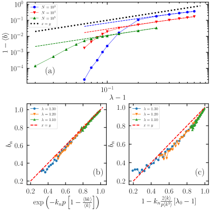
Figure 1: Comparison of $1-\left\langle{b}\right\rangle$ vs $\lambda=p\Lambda_{M}$ from numerical simulations for $\gamma=2.25$ (symbols), with QMF theoretical predictions based on Eq. (1) (dashed lines) for different values of $N$. (b) and (c): Comparison of $b_{n}$ from numerical simulations for various $\lambda=p\Lambda_{M}$ and $N=10^{4}$ with annealed network predictions, Eqs. (21) and (27), respectively. In (c), $\lambda_{0}=p\left\langle{k^{2}}\right\rangle/\left\langle{k}\right\rangle$ corresponds to the annealed network threshold.

In this Section we perform a systematic comparison between the results of the theoretical approaches presented in the previous Section and numerical results obtained by simulating the SIS dynamics on synthetic uncorrelated power-law distributed networks, built according to the Uncorrelated Configuration Model Catanzaro et al. (2005). The comparison is aimed at validating the accuracy of the theoretical predictions and at identifying the origin of possible inaccuracies in the various approximations performed. The networks considered have a degree distribution $P(k)\sim k^{-\gamma}$ between a minimum value $k_{min}=3$ and a maximum $k_{max}=N^{1/2}$ (for $\gamma<3$) and $k_{max}=N^{1/(\gamma-1)}$ for $\gamma>3$.

We consider as infinite all avalanches whose duration is longer than $t_{inf}=300$ steps. This threshold, chosen for computational convenience, is larger than the average duration of finite avalanches except for a narrow interval around the critical point. To improve the readability of figures, plotted values of $T_{n}$, $S_{n}$ and $b_{n}$ are binned over suitably chosen intervals.

We consider two values of $\gamma$ corresponding to the two different scenarios occurring for the SIS transition Pastor-Satorras et al. (2015). For $\gamma<5/2$ the transition is triggered by a subextensive network subset (the max K-core), composed of densely mutually interconnected nodes Castellano and Pastor-Satorras (2012). In this case QMF theory and the annealed network approximation are known to work well, providing an estimate of the position of the epidemic threshold which is asymptotically exact in the large size limit Ferreira et al. (2012); Silva et al. (2019). For $\gamma>5/2$ the epidemic transition is triggered by a different and highly nontrivial mechanism. Nodes with high connectivity (large hubs) considered together with their immediate neighbors, form star graphs. When $p$ becomes larger than $p_{c}^{QMF}=1/\Lambda_{M}\approx 1/\sqrt{k_{\mathrm{max}}}$ the largest of these star graphs becomes able to sustain epidemic activity for a long time, proportional to $\exp(k_{\mathrm{max}})$. For larger values of $p$ other star graphs can independently sustain activity. QMF theory describes only the behavior of isolated stars. However, the epidemic in each of them survives for a time proportional to $\exp(k_{i})$, i.e., there is no endemic activity in the system (surviving for a time $\exp(N)$) if stars are isolated Goltsev et al. (2012); Lee et al. (2013). As a consequence the QMF estimate $p_{c}^{QMF}=1/\Lambda_{M}$ is only a (not strict) lower-bound for the actual epidemic threshold. The consideration of long-range interactions among stars, neglected by QMF theory, allows to understand how endemic activity can be established and to calculate the actual critical threshold $p_{c}>p_{c}^{QMF}$ Boguñá et al. (2013); Castellano and Pastor-Satorras (2020).

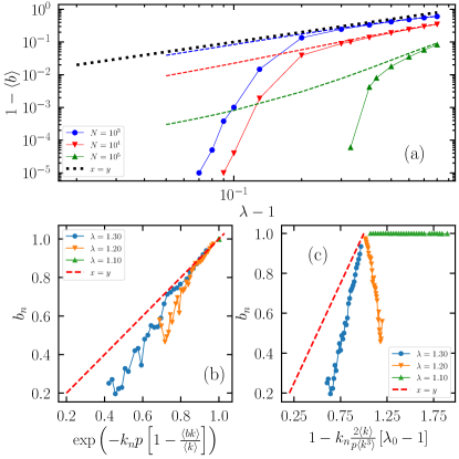
Figure 2: Comparison of $1-\left\langle{b}\right\rangle$ vs $\lambda=p\Lambda_{M}$ from numerical simulations for $\gamma=3.50$ (symbols), with QMF theoretical predictions based on Eq. (1) (dashed lines) for different values of $N$. (b) and (c): Comparison of $b_{n}$ from numerical simulations for various $\lambda=p\Lambda_{M}$ and $N=10^{4}$ with annealed network predictions, Eqs. (21) and (27), respectively. In (c), $\lambda_{0}=p\left\langle{k^{2}}\right\rangle/\left\langle{k}\right\rangle$ corresponds to the annealed network threshold.

III.0.1 Probability of observing a finite avalanche

In Fig. 1(a) we first compare the probability $1-\left\langle{b}\right\rangle$ of observing a finite avalanche calculated within the QMF approach [Eq. (1)] with numerical results for $\gamma=2.25$. It turns out clearly that QMF is very accurate in reproducing the behavior of $1-\left\langle{b}\right\rangle$. The bending of the numerical curves for small $\lambda-1$ is due to finite size effects reflecting the existence of a size-dependent effective threshold. As $N$ increases the agreement between theory and numerics extends to lower values of $\lambda-1$, confirming that the QMF threshold estimate is asymptotically exact Ferreira et al. (2012); Silva et al. (2019). The other two panels display instead the accuracy of the fully analytical predictions obtained when also the annealed network approximation is implemented. Also in this case we find a very good agreement between theory and simulations. Note that no parameter has been fitted.

In Fig. 2 the same analysis is performed for $\gamma=3.50$. The scenario is completely different. Also in this case the agreement between theory and simulations for what concerns $1-\left\langle{b}\right\rangle$ holds above a size-dependent threshold, but now the threshold moves toward larger values of $\lambda-1$ as $N$ is increased. This shows that the actual SIS threshold is larger than the QMF prediction, $\lambda_{c}>\lambda_{c}^{QMF}=1$, and the discrepancy grows with the system size Boguñá et al. (2013); Castellano and Pastor-Satorras (2020). The disagreement is even more evident in panels (b) and (c). In panel (b), all $b_{n}=1$ for $\lambda=1.1$ despite the QMF prediction that $b_{n}<1$ for $\lambda>\lambda_{c}^{QMF}=1$. This is a consequence of the fact that the true value of $\lambda_{c}$ is larger than 1.1, so that $\lambda=1.1$ is actually subcritical instead of supercritical. In panel (c) we have the additional complication that, when $\lambda=p\Lambda_{M}$ is 1.1 or 1.2, $\lambda_{0}=p\left\langle{k^{2}}\right\rangle/\left\langle{k}\right\rangle$ is smaller than 1. This gives rise to the unphysical values larger than 1 along the horizontal axis in Fig. 2(c).

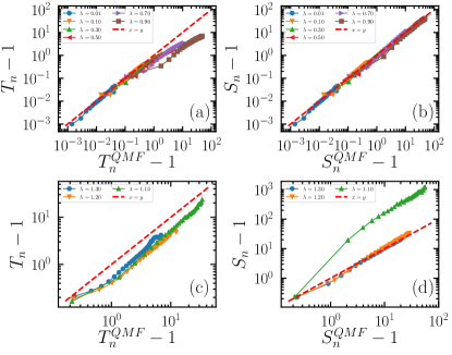
Figure 3: Comparison of numerical simulations with QMF theoretical predictions (Eqs. (9), and (16)) for $\gamma=2.25$ and $N=10^{4}$. (a) $T_{n}$ subcritical; (b) $S_{n}$ subcritical; (c) $T_{n}$ supercritical; (d) $S_{n}$ supercritical.

In summary, for $\gamma<5/2$ both QMF and annealed network theories predictions for the threshold are asymptotically exact, so that one expects theory and simulations to perfectly agree for large $N$. For $\gamma>5/2$ instead both theories predict a threshold value not matching numerics as $N$ grows. In that case the predictions for $b_{n}$ and $\left\langle{b}\right\rangle$ work only sufficiently inside the supercritical phase.

III.0.2 Average avalanche duration and size

In Fig. 3 we report a comparison between QMF predictions (along the horizontal axis) and numerical results (vertical axis) for $\gamma=2.25$. Results are presented for both the average duration $T_{n}$ (left column) and the average avalanche size $S_{n}$ (right column). In the subcritical case an excellent agreement is found for $S_{n}$ for any value of $\lambda$, while the same is true only for durations up to $T_{n}\approx 1$, corresponding to small values of $\lambda$. For larger durations a disagreement starts to appear for $T_{n}$. This difference can be rationalized based on the different treatments of Section II.1. The prediction for $S_{n}$ is valid for any size, without any small size assumptions. This failure of QMF theory in predicting the avalanche duration can be instead attributed to the breakdown of the assumption made to obtain Eq. (7). Close to the transition point, critical slowing down leads to a slow decay of $f_{n}(t)$ toward zero and it is not appropriate to assume linearization to hold starting from $t=1$.

For the average avalanche size in the supercritical case, Fig. 3(d), large discrepancies between theory and simulations occur for $\lambda$ slightly larger than 1, while an excellent agreement is found again for larger $\lambda$. This finding can be ascribed to the intrinsic impossibility of discriminating precisely finite or infinite avalanches in networks of finite size. At the critical point the distribution of avalanche times features a power-law decay plus incipient infinite avalanches, characterized by long but still finite durations. Some of them are classified as finite according to the criterion $T<t_{inf}$ and therefore contribute to $T_{n}$ increasing its value by a large amount. Reducing $t_{inf}$ alleviates this problem, but at the price of risking to spuriously consider as infinite avalanches those belonging to the power-law decay. This difficulty is naturally mitigated by considering larger systems, or going to larger $\lambda$, as the separation between the two components of the duration distribution becomes more pronounced. For the average avalanche duration in the supercritical case, Fig. 3(c) this intrinsic problem with finite size (which tends to increase $T_{n}$) competes with the breakdown of the linearization for $f_{n}$ (which tends to decrease $T_{n}$). As a consequence, numerical results are not far from QMF predictions.

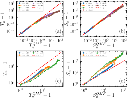
Figure 4: Comparison of numerical simulations with theoretical predictions (Eqs. (9), and (16)) for $\gamma=3.50$ with $N=10^{4}$. (a) $T_{n}$ subcritical; (b) $S_{n}$ subcritical; (c) $T_{n}$ supercritical; (d) $S_{n}$ supercritical.

Figure 4 reports the same analysis for $\gamma=3.50$; the same qualitative scenario emerges concerning the agreement between QMF theory and simulations. This is somewhat surprising, given the known failure of QMF in describing accurately the transition in this case. However, this failure becomes most evident for very large networks, while only moderate values of $N$ are considered here Silva et al. (2019).

Further insight into what happens for long subcritical avalanches close to the threshold is provided in Fig. 5, where we plot the average avalanche size versus the corresponding duration, obtained from numerical simulations. As we can see here, for small values of $\lambda$, the QMF prediction $S_{n}\sim T_{n}$ is well fulfilled. Closer to the critical point, on the other hand, we observe a departure from the linear behavior, which reflects the mismatch between the poor agreement with the QMF theory for large $\lambda$ of the avalanche duration $T_{n}$ and the very good agreement of the avalanche size $S_{n}$. Numerically, we observe instead a good fit for $\lambda$ close to $1$ to the form $S_{n}\sim T_{n}^{2}$, see Fig. 5(c) and (d), which is a consequence of the critical scalings of $p_{n}(s)$ and $p_{n}(t)$ Larremore et al. (2012).

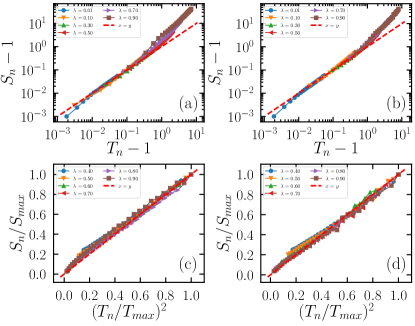
Figure 5: Plot of the avalanche size $S_{n}$ as a function as the avalanche duration $T_{n}$ for $\gamma=2.25$ (a) and $\gamma=3.50$ (b) in the subcritical regime. Panels (c) and (d) show the avalanche size $S_{n}$ (normalized by its maximum value) as a function of the square of the avalanche duration $T_{n}$ normalized by its maximum value), for $\gamma=2.25$ and $\gamma=3.50$, respectively. Data from numerical simulations in networks of size $N=10^{4}$.

Figures 6 and 7 analyze instead the agreement between simulations and the theoretical results obtained using the annealed network approximation, for both $T_{n}$ [Eqs. (35) and (39)] and $S_{n}$ [Eqs. (41) and (42)].

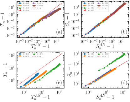
Figure 6: Comparison of numerical simulations with annealed network predictions for $\gamma=2.25$ and $N=10^{4}$. (a) $T_{n}$ subcritical (Eq. (35)); (b) $S_{n}$ subcritical (Eq. (41)); (c) $T_{n}$ supercritical (Eq. (39)); (d) $S_{n}$ supercritical (Eq. (42)).

For $\gamma=2.25$ we find a very good agreement throughout the whole phase-diagram, except for a critical region around the epidemic threshold. For $\gamma=3.50$, the fit is very good in the subcritical regime, and rather poor away from the critical point in the supercritical regime. This is due to the fact that the annealed network threshold $p_{c}^{ann}$ largely overestimates the actual threshold. A consequence of this overestimate is that for $\lambda$ slightly larger than 1, Eqs. (39) and (42) predict negative values of $T_{n}$ and $S_{n}$. A better agreement between theory and numerical results is expected for larger values of $\lambda$, which will be less affected by the mismatch between the prediction of the threshold and its actual value.

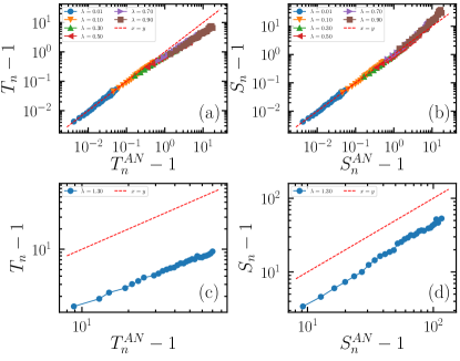
Figure 7: Comparison of numerical simulations with annealed network predictions for $\gamma=3.50$ and $N=10^{4}$. (a) $T_{n}$ subcritical (Eq. (35)); (b) $S_{n}$ subcritical (Eq. (41)); (c) $T_{n}$ supercritical (Eq. (39)); (d) $S_{n}$ supercritical (Eq. (42)).

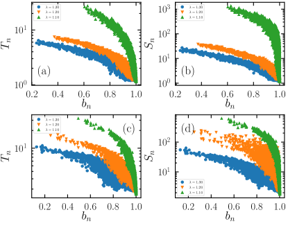
Figure 8: Dependence of the avalanche average duration and size as a function of the $b_{n}$ in the supercritical regime. (a) $T_{n}$ and (b) $S_{n}$ for $\gamma=2.25$. (c) $T_{n}$ and (d) $S_{n}$ for $\gamma=3.50$.

Finally, in Fig. 8 we report the dependence of the average avalanche duration $T_{n}$ and size $S_{n}$ in the supercritical regime, as a function of the probability of observing a finite avalanche $b_{n}$. For both $\gamma=2.25$ and $\gamma=3.50$, we find continuously decreasing functions of $b_{n}$, with large but not huge fluctuations. The monotonicity allows us to assume, as a rule of thumb, that if a node has a larger probability $1-b_{n}$ to originate an infinite avalanche than a second node, the first will also give rise on average to longer and larger finite avalanches. In other words, ranking nodes according to $b_{n}$, $T_{n}$ or $S_{n}$ produces the same ordering, apart from fluctuations.

IV Conclusions

In this paper we present a thorough investigation, both analytical and numerical, of the problem of identifying influential spreaders for SIS dynamics on generic networks. We first apply to this problem the theoretical QMF framework introduced by Larremore et al. in Ref. Larremore et al. (2012). In this way we are able to write down closed equations, whose numerical solution allows us to calculate all the observables of interest in the whole phase-diagram. Within this approach a further step, consisting in the implementation of the annealed network approximation, allows us to derive explicit analytical predictions valid below and above (but close to) the critical point. These predictions point out the importance of degree centrality in determining the spreading influence. Comparison of these results with analytical simulations, performed on synthetic networks with power-law distributed degrees $P(k)\sim k^{-\gamma}$, confirms the substantial accuracy of the theoretical approaches below the threshold, in particular for what concerns the avalanche size. Above the expected QMF threshold discrepancies arise, which tend to disappear inside the active region of the phase-diagram.

Let us discuss in detail strengths and limitations of the theoretical approaches considered here. The QMF theory of Larremore et al. Larremore et al. (2012) is based on three approximations: The neglect of dynamical correlations among neighbors’ states; the locally tree-like assumption that allows to write down Eqs. (1) and (2); the linearization entailed in Eq. (3) for the derivation of $T_{n}$. The annealed network approximation adds another assumption on top of them. For strongly heterogeneous unclustered networks, such as those generated by the Uncorrelated Configuration Model with $\gamma<5/2$, the first two assumptions are essentially correct. Studies on SIS dynamics have shown that even the annealed network approximation works very well in this case. The linearization holds instead only if one is sufficiently far from the epidemic threshold. Close to it, the regime with exponential decay into the stationary state is preceded by a long transient during which the decay is power-law (critical slowing down), $f_{n}$ is not small and linearization does not hold; the dominating contribution to the overall duration of avalanches comes from this long preasymptotic regime. For this reason predictions for $T_{n}$ are not consistent with simulations, for values of $p$ close to the threshold. When $\gamma>5/2$, the agreement between our theoretical results and simulations is expected to be poorer. The reason is that already the first approximation, the neglect of dynamical correlations, fails to capture the complex physical mechanisms underlying the epidemic transition and thus introduces large errors. See Ref. Pastor-Satorras et al. (2015) for more on this. A fundamental consequence is that already the QMF estimate of the epidemic threshold is qualitatively and quantitatively incorrect. This leads to the expectation that predictions for influential spreaders in the supercritical case are largely off target. The relatively small errors observed here are believed to be an effect of the relatively small network sizes considered. The additional annealed network approximation, which does not work for $\gamma>5/2$, makes the theoretical approaches perform even worse. Recent results Castellano and Pastor-Satorras (2020) have pointed out the great complexity of the physical mechanisms underlying the epidemic transition in random networks with $\gamma>5/2$. This understanding constitutes the necessary groundwork for reaching a satisfactory predictive ability for influential spreaders also in this case, a goal that remains to be reached. Similarly, the extension of this approach to networks exhibiting more complicated features, such as clustering, correlations or mesoscopic structures, remains an interesting open issue.

Finally, it is worth remarking that our results have been derived for a particular, discrete-time, version of SIS dynamics, rather different from the usual continuous-time version. The present version, with parallel dynamics and recovery time fixed to 1, allows a freshly infected node to immediately reinfect the node that infected it in the preceding time step. This kind of process is instead strongly hindered in continuous-time SIS, where the neighbor $j$ that infected node $i$ remains infected for a while so that the number of connections of $i$ available for further spreading is effectively $k_{i}-1$. This kind of dynamical correlations has strong effects for influential spreaders in SIR dynamics. In that case degree centrality is a good approximation of the spreading influence of individual nodes, but close to the transition a better approximation is provided by the non-backtracking centrality Martin et al. (2014); Radicchi and Castellano (2016); Min (2018), which may differ markedly from the former. The quest for accurate predictors of spreading influence for continuous-time SIS dynamics close to the transition is an interesting open avenue for further research.