Luminous Red Novae: population models and future prospects

Abstract

A class of optical transients known as Luminous Red Novae (LRNe) have recently been associated with mass ejections from binary stars undergoing common-envelope evolution. We use the population synthesis code COMPAS to explore the impact of a range of assumptions about the physics of common-envelope evolution on the properties of LRNe. In particular, we investigate the influence of various models for the energetics of LRNe on the expected event rate and light curve characteristics, and compare with the existing sample. We find that the Galactic rate of LRNe is $\sim 0.2$ yr^-1, in agreement with the observed rate. In our models, the luminosity function of Galactic LRNe covers multiple decades in luminosity and is dominated by signals from stellar mergers, consistent with observational constraints from iPTF and the Galactic sample of LRNe. We discuss how observations of the brightest LRNe may provide indirect evidence for the existence of massive ($>40$ M_⊙) red supergiants. Such LRNe could be markers along the evolutionary pathway leading to the formation of double compact objects. We make predictions for the population of LRNe observable in future transient surveys with the Large Synoptic Survey Telescope and the Zwicky Transient Facility. In all plausible circumstances, we predict a selection-limited observable population dominated by bright, long-duration events caused by common envelope ejections. We show that the Large Synoptic Survey Telescope will observe $20$–$750$ LRNe per year, quickly constraining the luminosity function of LRNe and probing the physics of common-envelope events.

1 Introduction

Common-envelope evolution (Paczynski, 1976) is a phase of mass transfer in the evolution of many stellar binaries, wherein the two stars or stellar cores orbit inside a shared gas envelope. The resulting drag force causes significant energy dissipation and a rapid decay of the binary’s orbit. The outcome is either a stellar merger or, if the envelope is successfully ejected, a binary with a much-reduced separation. The common-envelope phase is thought to be an important evolutionary channel for the formation of X-ray binaries, binary pulsars, and gravitational-wave sources such as merging double white dwarfs, binary neutron stars, and double black holes (e.g. Smarr & Blandford, 1976; van den Heuvel, 1976; Tutukov & Yungelson, 1993; Voss & Tauris, 2003; Dominik et al., 2012; Belczynski et al., 2016; Stevenson et al., 2017; Vigna-Gómez et al., 2018).

The short duration of the common envelope phase makes catching a binary during this process observationally challenging. Recently, a class of optical transients in the luminosity gap between novae and supernovae known as Luminous Red Novae (LRNe) have been associated with common-envelope evolution (Soker & Tylenda, 2003; Kulkarni et al., 2007; Tylenda et al., 2011; Ivanova et al., 2013b; Pastorello et al., 2019). These transients are characterised by a rapid rise in luminosity followed by a lengthy plateau, often with a secondary maximum which may be powered by the shock collision of the expanding shell with previously ejected material (Metzger & Pejcha, 2017). The best evidence for the association of LRNe with common-envelope evolution comes from the observed orbital decay of the Galactic binary V1309 Sco over ten years (Tylenda et al., 2011) preceeding a LRN outburst. Soker & Tylenda (2003), Kulkarni et al. (2007), Tylenda et al. (2011), and Williams et al. (2015) have suggested that LRNe may be due to stellar mergers, while Blagorodnova et al. (2017) proposed that the LRN M101 OT2015-1 was produced by the ejection of a common envelope from a binary involving a massive star. Pastorello et al. (2019) presented photometric and spectroscopic data on several bright LRNe and LRN candidates, finding that the ejection of a common-envelope was the most favoured origin of these transients.

Event Name	Duration [days]	$L/L_{\odot}$
V838 Mon (G)	$70\pm 10$	$(1\pm 0.2)\times 10^{6}$	Tylenda (2005)
V1309 Sco (G)	$20\pm 10$	$(2.5\pm 0.5)\times 10^{4}$	Tylenda et al. (2011)
M85-OT (E)	$70\pm 10$	$(5\pm 1)\times 10^{6}$	Kulkarni et al. (2007); Pastorello et al. (2007); Rau et al. (2007); Ofek et al. (2008)
NGC 4490$-$2011OT1 (E)	$200\pm 40$	$(3\pm 1)\times 10^{7}$	Smith et al. (2016); Pastorello et al. (2019)
M31 2015 (E)	$30\pm 10$	$8.7^{+3.3}_{-2.2}\times 10^{5}$	Kurtenkov et al. (2015); Williams et al. (2015); MacLeod et al. (2017)
M31 RV 1988 (E)	$30\pm 10$	$(8\pm 2)\times 10^{5}$	Mould et al. (1990)
M101 OT2015 (E)	$100\pm 20$	$(2.5\pm 1)\times 10^{6}$	Goranskij et al. (2016); Blagorodnova et al. (2017); Lipunov et al. (2017); Pastorello et al. (2019)
NGC 3437$-$2011OT1 (E)	$100\pm 20$	$(1\pm 0.3)\times 10^{7}$	Pastorello et al. (2019)
UGC 12307$-$2013OT1 (E)	$50\pm 20$	$(2\pm 0.5)\times 10^{7}$	Pastorello et al. (2019)
SNhunt248 (E)	$110\pm 20$	$(2\pm 1)\times 10^{7}$	Kankare et al. (2015); Mauerhan et al. (2018); Pastorello et al. (2019)
AT 2017jfs (E)	$140\pm 20$	$(3\pm 1)\times 10^{7}$	Pastorello et al. (2019)
AT 2018hso (E)	$100\pm 20$	$(1\pm 0.3)\times 10^{7}$	Cai et al. (2019); Pastorello et al. (2019)
SN 1997bs (E)	$60\pm 20$	$(4\pm 2)\times 10^{6}$	Van Dyk et al. (2000); Pastorello et al. (2019)

Table 1: Summary of observed LRNe with reliably inferred absolute plateau luminosities and durations. Events labelled (G) occurred within the Galaxy and events labelled (E) were of extragalactic origin.

To date, there have been 13 observations of LRNe with recorded plateau durations and accurate distance estimates allowing inference on the absolute magnitude. We summarise these in Table 1, including the characteristic luminosities and durations of the plateaux, as well as whether they are of Galactic or extra-galactic origin. Where plateau durations are not stated in the discovery papers, we estimate them from the light curves as the time over which the brightness decreases by approximately one magnitude (either $V$-band where given or absolute) from the peak. In the case of V838 Mon, NGC 4490-OT2011, and M101 OT2015, which have a double-peaked lightcurve, we use the time between the first and second maxima to estimate the duration. All luminosities quoted in table 1 are taken from the original references cited, or converted from bolometric magnitudes, with the exception of M85–OT, where we use the luminosity in the R band from Kulkarni et al. (2007). Error ranges are approximate and are determined by eye. Some events described as possible LRNe in the literature, such as V4332 Sgr (Martini et al., 1999; Kimeswenger, 2006), have been omitted in our analysis; their absolute magnitude is not known, and so we cannot compare their properties to our simulated population of LRNe. There are other optical transients with similar luminosities to LRNe. These contribute a source of confusion noise to the population of LRNe with a possibly different physical mechanism behind the transient. We do not regard SN2008S (Arbour & Boles, 2008), NGC 300 OT 2008 (Berger et al., 2009; Prieto et al., 2009; Bond et al., 2009) and M51 OT2019-1 (Jencson et al., 2019) as LRNe, but rather as likely Type IIn electron capture supernovae (Prieto et al., 2008; Adams et al., 2016). We also neglect the luminous infra-red transient VVV-WIT-06, which is most likely an obscured classical nova (Banerjee et al., 2018). Nova Vul 1670 has been suggested as a possible historical example of a LRN (Kamiński et al., 2015), however we do not include it in our present sample. Due to its unusual light curve, we also exclude OGLE-2002-BLG-360 (Tylenda et al., 2013) from our subsequent analysis. We exclude LRN PTF 10FQS from our sample; it is likely this is an intermediate-luminosity red transient, and not an LRN (Kasliwal et al., 2011; Pastorello et al., 2019). On the other hand, we include the transient UGC 12307–2013OT1 in our sample, despite the uncertainty over its classification, owing to its late discovery (Pastorello et al., 2019); its inclusion in our sample does not affect the findings of this paper. In the future, better models and larger statistical samples could make it possible to use tools such as those introduced by Farr et al. (2015) for counting amid confusion to avoid making binary cuts on potential LRN candidates.

As Table 1 shows, the current scarcity and diversity of LRN observations makes extracting information about the intrinsic population of these transients and their progenitors difficult, though some progress has been made. The unusually luminous extragalactic LRN NGC 4490-OT2011 has been identified with a merger involving a massive blue progenitor (Smith et al., 2016). Within our Galaxy, only four likely LRNe have been detected in approximately 25 years: V4332 Sgr, V1309 Sco, V838 Mon, and tentatively OGLE-2002-BLG-360 (though see above). The Large Synoptic Survey Telescope (LSST) will observe $\sim$20,000 deg² with a cadence of $\sim 3$ days down to a single-visit limiting $r$-band magnitude of $\approx 24.2$ (LSST Science Collaboration et al., 2017), and is expected to increase the number of detected LRNe by several orders of magnitude (LSST Science Collaboration et al., 2009).

In this paper, we use the binary population synthesis code COMPAS (Stevenson et al., 2017; Barrett et al., 2018; Vigna-Gómez et al., 2018; Neijssel et al., 2019) and a model of LRN plateau durations and luminosities from Ivanova et al. (2013b) to predict what the properties of this observed population will be under a variety of models of common envelope interaction. We find that the Galactic rate of LRNe is $\approx 0.1$ yr^-1, consistent with observations and previous population studies. We predict that the volumetric rate in the local Universe is $\approx 8\times 10^{-4}$ Mpc^-3 yr^-1, and that with LSST the rate of LRN detections could be as high as 750 yr^-1.

The rest of this paper is structured as follows. In section 2.1 we introduce the population synthesis code COMPAS, which we use to simulate a catalogue of common-envelope events. In section 2.2, we describe how mass transfer, including common-envelope evolution, is implemented within COMPAS. In section 2.3 we describe the parameters of the simulations used in this paper. In section 2.4 we summarise the formalism that we employ for predicting the observable properties of LRNe. In section 3.1 we present the results of the population synthesis simulation and compare to previous work. In sections 3.2 and 3.3 we present our predictions for the observable properties and rates of LRNe, respectively. We discuss these results in section 4.

2 Methods

2.1 Population synthesis

In order to predict the rate and properties of common-envelope events, we simulate a large stellar population using the rapid population synthesis module of COMPAS (Stevenson et al., 2017; Barrett et al., 2018; Vigna-Gómez et al., 2018; Neijssel et al., 2019). The COMPAS binary population synthesis module simulates a population of binaries by Monte Carlo sampling a distribution of initial (ZAMS) binary masses and separations, then evolving each star in the binary according to the single-stellar evolution prescription of Hurley et al. (2000). COMPAS evolves each binary by modelling the physics of mass loss and transfer due to effects such as stellar winds, Roche lobe overflow and supernovae, until the binary either merges, becomes unbound, or forms a double compact object. We describe in detail how mass transfer during binary evolution is implemented in COMPAS below.

The version of COMPAS used in this paper, and the parameters used in our simulation, are similar to those described in Vigna-Gómez et al. (2018). Where substantive changes have been made to either we describe these explicitly in text.

2.2 The common envelope

In the COMPAS models, a Roche-lobe overflow mass transfer episode begins when the radius of one of the star becomes larger than the effective radius of its Roche lobe (Eggleton, 1983). This may occur due to radial expansion of a star, orbital evolution of the binary, or both.

A mass transfer episode either ends with the system gently decoupling from Roche-lobe overflow, or mass loss from the donor leads to a runaway process. The first of these scenarios, dynamically stable mass transfer, occurs on either the nuclear or thermal timescale of the donor. In the second scenario, dynamical instability leads to the formation of a common envelope, with subsequent inspiral on the dynamical timescale (Paczynski, 1976).

The stability of mass transfer is determined in COMPAS using the mass-radius relationship, $\zeta=d\log R/d\log M$, in order to quantify how the radius responds to mass loss (Soberman et al., 1997; Tout et al., 1997). We compare the adiabatic mass-radius coefficient of the donor star $\zeta_{\rm{ad}}$ to the Roche-lobe mass-radius coefficient of the binary $\zeta_{\rm{RL}}$. The latter is computed under the assumption of stable mass transfer, with the amount of angular momentum lost from the system given by the fiducial COMPAS model, as described in section 2.3.1 of Neijssel et al. (2019). In order for the mass transfer episode to be dynamically stable, we require $\zeta_{\rm{ad}}\geq\zeta_{\rm{RL}}$. If this condition is not satisfied, mass transfer is assumed to be unstable on a dynamical timescale and leads to a common-envelope phase. We use the choices and implementation of $\zeta_{\rm{ad}}$ from Vigna-Gómez et al. (2018), informed in part by quantitative comparisons to observations of Galactic double neutron stars and merging binary black holes. In addition to the standard picture of a common envelope described above, these choices are intended to phenomenologically account for common envelopes initiated by the expansion of the accretor beyond its Roche lobe in response to rapid mass transfer (Nariai & Sugimoto, 1976).

For main-sequence (MS) and Hertzsprung-Gap (HG) donors, we use fixed values of $\zeta_{\rm{ad,MS}}=2.0$ and $\zeta_{\rm{ad,HG}}=6.5$, respectively. These mass-radius relations represent roughly average typical values for these phases, following adiabatic mass-loss models from Ge et al. (2015). The prescription for HG donors is an effective value intended to describe delayed dynamical instability (Hjellming & Webbink, 1987), rather than incipient Roche-lobe overflow from a radiative HG donor. For core-helium burning and giant stars we use a fit for condensed polytropes with convective envelopes presented in Soberman et al. (1997), $\zeta_{\rm{ad}}=\zeta_{\rm{SPH}}$. Finally, for stripped stars, such as naked helium, helium-shell-burning or helium giant stars, we assume mass transfer to always be stable; this results in having no LRNe from these stripped donors in our model.

2.2.1 Common-envelope evolution

The common-envelope phase remains a poorly understood key aspect of binary evolution. We use the standard assumption that if $\zeta_{\rm{ad}}<\zeta_{\rm{RL}}$, mass transfer is unstable and leads to a common-envelope phase (Paczynski, 1976). However, the stability threshold is uncertain: for example, apparent initial instability for HG donors could resolve into stable mass transfer (Pavlovskii et al., 2017).

It is predicted to lead to a significant tightening of the binary, and thus contribute to both stellar mergers and double compact object formation (see, e.g., discussion in Ivanova et al., 2013a). The common-envelope phase is initiated when unstable mass transfer allows the envelope of the donor to engulf the companion as well as the core of the donor, so that both stars/stellar cores orbit inside the recently formed common envelope. The binary formed by the companion and the donor’s core is not in co-rotation with the envelope. Viscous shear and tidal interactions with the envelope cause the companion to inspiral. This inspiral liberates orbital energy. If the released energy is large enough, and is effectively transferred to the envelope, the envelope may be ejected; otherwise, the system merges. The conditions that are assumed to lead to either envelope ejection or stellar merger within the envelope are discussed below.

2.2.2 Energy formalism

In the classic energy $\alpha$-formalism for the common envelope (Iben & Tutukov, 1984; Webbink, 1984, 2008; De Marco et al., 2011; Ivanova et al., 2013a), the change in orbital energy during the phase is compared to the binding energy required to eject the envelope to infinity. The difference in the initial and final orbital energies is given by

$$\Delta E_{\mathrm{orb}}=E_{\mathrm{initial}}-E_{\mathrm{final}}=\left(-\frac{GM_{1}M_{2}}{2a_{\mathrm{initial}}}+\frac{GM_{1,c}M_{2}}{2a_{\mathrm{final}}}\right),$$ (1)

where $a_{\mathrm{initial}}$ and $a_{\mathrm{final}}$ are the initial and final orbital separations respectively, $M_{1}$ and $M_{2}$ are the initial masses of the two stars and $M_{1,c}$ is the core mass of the donor after its envelope is removed. The parameter $\alpha$ characterises the efficiency with which the orbital energy is used to eject the envelope whose initial binding energy is $E_{\mathrm{bind}}$:

$$\alpha\Delta E_{\mathrm{orb}}=E_{\mathrm{bind}}\,.$$ (2)

If the binding and orbital energies are the only energies involved in the common envelope interaction, then $0\leq\alpha\leq 1$. There are, however, additional possible energy sources not taken into account in the classical definition, such as recombination energy (Nandez & Ivanova, 2016) or enthalpy (Ivanova & Chaichenets, 2011), which allow for $\alpha>1$. Other recent work suggests that $\alpha<0.6$–1.0 (Iaconi & De Marco, 2019). Generally speaking, a higher value of $\alpha$ leads to more binaries surviving the common-envelope phase, while a lower value leads to more mergers during common-envelope evolution. In this paper, we assume $\alpha=1$, although this assumption technically violates energy conservation in some of the models for ejecta kinetic energy described below. To check the impact of the assumed value of $\alpha$ on our results, we repeat a population synthesis simulation with $\alpha=0.5$. We discuss the effects of modifying this assumption in section 3.1.

The binding energy of the envelope $E_{\mathrm{bind}}$ can be calculated from detailed stellar models for single stars (e.g. Dewi & Tauris, 2000; Xu & Li, 2010a; Loveridge et al., 2011; Ivanova, 2011; Wang et al., 2016; Kruckow et al., 2016). The main source of uncertainty in calculating the binding energy is in determining the core-envelope boundary (e.g. Tauris & Dewi, 2001; Ivanova, 2011). In COMPAS, we use the parameter $\lambda$ (de Kool et al., 1987) to characterise the binding energy of a stellar envelope, so we can re-write Equations 1 and 2 as (Ivanova et al., 2013a)

$$\frac{GM_{1}M_{1,\mathrm{env}}}{\lambda R_{1}}=\alpha\left(-\frac{GM_{1}M_{2}}{2a_{\mathrm{initial}}}+\frac{GM_{1,\mathrm{c}}M_{2}}{2a_{\mathrm{final}}}\right)\,,$$ (3)

where $R_{1}$ is the radius of the donor before the interaction. Equation 3 assumes that only the donor star has a core-envelope separation. If the companion also has an envelope, then we assume that unstable mass transfer from either star triggers a ‘double-core common envelope’, in which case Equation 3 becomes

$$\frac{M_{1}M_{1,\mathrm{env}}}{\lambda_{1}R_{1}}+\frac{M_{2}M_{2,\mathrm{env}}}{\lambda_{2}R_{2}}=\alpha\left(-\frac{GM_{1}M_{2}}{2a_{\mathrm{initial}}}+\frac{GM_{1,\mathrm{c}}M_{2,\mathrm{c}}}{2a_{\mathrm{final}}}\right)\,.$$ (4)

In this work, we follow Vigna-Gómez et al. (2018) in computing $\lambda$ using fitting formulae to the detailed stellar structure models of Xu & Li (2010a); Xu & Li (2010b). In order to determine whether a common envelope interaction results in a merger or the ejection of the envelope, we solve Equation 3 or 4 for $a_{\mathrm{final}}$. If both stars or stellar cores fit within their Roche lobes at the end of the common-envelope phase, we assume that the envelope has been ejected; otherwise, we assume that the stars merge.

2.2.3 Common-envelope evolution in COMPAS

COMPAS does not directly simulate the common-envelope interaction – such simulations are difficult and expensive even for single systems – and so our implementation contains several prescriptive assumptions for how common-envelope evolution proceeds. Here we list several key assumptions that may differ between this work and other population synthesis studies.

• If the donor during a common-envelope phase is a MS star, the result is always a stellar merger.

• The main change from the version of COMPAS used for Vigna-Gómez et al. (2018) is that MS accretors are allowed to engage in and survive a common-envelope phase. Previously, dynamically unstable mass transfer onto MS accretors was assumed to inevitably lead to mergers, which is still the case for MS donors. This change leads to a higher rate of common-envelope ejections compared to the previous model.

• Some studies suggest that HG stars do not have a clear core/envelope separation, so unstable mass transfer involving HG donors should always lead to mergers (Belczynski et al., 2007; Dominik et al., 2012), similarly to MS donors. We flag these systems and follow their evolution. If we assume that a HG donor has a clear core/envelope separation, we evolve the system by following the common-envelope energy formalism described above, in what is referred to as the “optimistic” variant. Alternatively, the system always merges in the “pessimistic” variant. We examine the impact of these variants on our results in section 3.

• If the stripped core overflows its Roche lobe immediately after the common envelope is ejected, we assume that the binary does not successfully emerge from the common-envelope phase and the stars merge.

2.3 Simulation parameters

For our model population, we evolve $5\times 10^{5}$ binary systems. We draw the mass of the primary from the Kroupa initial mass function (IMF) (Kroupa, 2001), with $1.0M_{\odot}\leq M_{1}\leq 100M_{\odot}$. The lower mass limit is chosen so that we only simulate systems in which the primary will evolve off the main sequence within approximately the age of the Universe. We neglect the effect of magnetic braking in low mass stars. The upper mass limit is chosen due to the uncertainty of stellar evolution models in the high mass range. We take our ZAMS mass cut into account when we normalise our simulated event rates by the total star formation rate. The secondary mass is determined by drawing a mass ratio from a flat distribution (Sana et al., 2012), with a minimum secondary mass of $0.1M_{\odot}$, corresponding to the brown dwarf limit (Kumar, 1963; Hayashi & Nakano, 1963). The initial binary separation is drawn from a flat-in-the-log distribution with $0.01\,\mathrm{AU}\leq a\leq 1000\,\mathrm{AU}$ (Abt, 1983). While it is possible that binary systems may be born with separations as wide as $10^{5}\mathrm{AU}$, these are not expected to interact and can be accounted for through normalisation. In fact, only around half of the systems we simulate undergo any form of mass transfer within a Hubble time.

Moe & Di Stefano (2017) inferred a more complex distribution of binary initial conditions from observations, with correlations between component masses, orbital separations, and birth eccentricities. Klencki et al. (2018) compared the impact of the Moe & Di Stefano (2017) initial conditions against initial conditions similar to the ones we assumed here on the merger rate of double compact objects, and found that the effect of changing the initial distribution was generally well within other modelling uncertainties. Therefore, we opt for the simpler, non-correlated initial conditions in this study, but caution that this is one of several sources of uncertainty.

The initial conditions used in this simulation We use a global “solar” metallicity of $Z=0.0142$ (Asplund et al., 2009). In this work, we assume a continuous, constant-rate star formation of infinite duration; we discuss the effect of this assumption and the binary fraction/separation completeness further in section 4.

2.4 Luminous red novae

To determine the observational properties of LRNe resulting from common envelope interactions in our population synthesis simulations, we follow Ivanova et al. (2013b), and adapt the scaling relations of Popov (1993) and Kasen & Woosley (2009), derived for type IIP supernovae, to estimate the luminosity and duration of the LRN plateau:

$$L_{p}=1.7\times 10^{4}L_{\odot}\left(\frac{R_{\mathrm{init}}}{3.5\,R_{\odot}}\right)^{2/3}\left(\frac{E_{\mathrm{k}}^{\infty}}{10^{46}\,\mathrm{erg}}\right)^{5/6}\\ \left(\frac{M_{\mathrm{unb}}}{0.03\,M_{\odot}}\right)^{-1/2}\left(\frac{\kappa}{0.32\,\mathrm{cm}^{2}\,\mathrm{g}^{-1}}\right)^{-1/3}\left(\frac{T_{\mathrm{rec}}}{4500\,\mathrm{K}}\right)^{4/3},$$ (5)

$$t_{p}=17\,\mathrm{days}\left(\frac{R_{\mathrm{init}}}{3.5\,R_{\odot}}\right)^{1/6}\left(\frac{E_{\mathrm{k}}^{\infty}}{10^{46}\,\mathrm{erg}}\right)^{-1/6}\\ \left(\frac{M_{\mathrm{unb}}}{0.03\,M_{\odot}}\right)^{1/2}\left(\frac{\kappa}{0.32\,\mathrm{cm}^{2}\,\mathrm{g}^{-1}}\right)^{1/6}\left(\frac{T_{\mathrm{rec}}}{4500\,\mathrm{K}}\right)^{-2/3},$$ (6)

where $R_{\mathrm{init}}$ is the Roche lobe radius of the donor star prior to the common envelope phase (or the binary separation in the case of double-core common envelope events), $E_{\mathrm{k}}^{\infty}$ is the kinetic energy of the ejected material after it escapes the gravitational potential well, $M_{\mathrm{unb}}$ is the mass of the ejected material, $\kappa$ is the opacity of the ionized ejecta, and $T_{\mathrm{rec}}$ is the recombination temperature.

In this work, we use as fiducial values $\kappa=0.32\,\mathrm{cm}^{2}\,\mathrm{g}^{-1}$ and $T_{\mathrm{rec}}=4500\,\mathrm{K}$. We parametrize $M_{\mathrm{unb}}=f_{\mathrm{m}}M_{\mathrm{env}}$, where $0\leq f_{\mathrm{m}}\leq 1$ and $M_{\mathrm{env}}$ is the mass of the envelope. We assume $f_{\mathrm{m}}=1$ for successful common envelope ejection, corresponding to the total expulsion of the envelope. We explore the effect of varying values of $f_{\mathrm{m}}$ for common envelope interactions leading to stellar mergers in section 3, where we consider $f_{\mathrm{m}}=0.05$ and $f_{\mathrm{m}}=0.5$. Some binaries ($\approx 6\%$) in our simulation undergo merger while both stars are still on the main sequence, before either has developed a core/envelope separation. Simulations of stellar mergers by direct collision find that $\approx 1-10\%$ of the total mass may be lost (Lombardi et al., 2002; Glebbeek et al., 2013). Simulations of stellar mergers due to unstable mass transfer in binaries have also shown that a few percent of the primary mass is ejected (Nandez et al., 2014). We model MS-MS mergers in the same way as mergers resulting from a common-envelope interaction, but taking $M_{\mathrm{env}}$ to be 25$\%$ of the total mass of the binary; for $f_{\mathrm{m}}=0.05$ (0.5), this corresponds to 1.25% (12.5%) of the total MS-MS binary’s mass being ejected during a merger, so the two variants we consider likely bracket the true value.

2.5 Ejecta kinetic energy

The kinetic energy of the ejecta $E_{\mathrm{k}}^{\infty}$ is the most poorly determined quantity in equations 5 and 6. We consider several prescriptions for calculating $E_{\mathrm{k}}^{\infty}$:

1. As the default model, we use the original prescription from Ivanova et al. (2013b), who assume that the kinetic energy of the ejecta is proportional to the gravitational potential energy of the ejected material at the donor’s surface before the interaction,

   $$E_{\mathrm{k}}^{\infty}=\zeta(GM_{\mathrm{unb}}M)/R_{\mathrm{init}}\,,$$ (7)

   where $M$ is the mass of the donor, or, for a double-core common-envelope, the total mass in the binary. Ivanova et al. (2013b) consider several values of $\zeta$; here we use $\zeta=10$ for ejections and $\zeta=1$ for mergers. This implies ejecting the material with $v_{\infty}=\sqrt{\zeta}v_{\mathrm{esc,don}}$, where $v_{\mathrm{esc,don}}$ is the escape velocity from the surface of the donor. If we enforce conservation of energy, $\Delta E_{\mathrm{orb}}=E_{\mathrm{k}}^{\infty}+E_{\mathrm{bind}}$, this variant corresponds to a variable $\alpha$ given by $\alpha=1/(1+\zeta\lambda)$, although we use a fixed $\alpha=1$ to determine whether the binary is able to eject the envelope in all variants for consistency.

2. We assume that the velocity of the ejected material is the same as the escape velocity from the binary, so that

   $$E_{\mathrm{k}}^{\infty}=\frac{1}{2}M_{\mathrm{unb}}v_{\mathrm{esc,bin}}^{2}=\frac{GM_{\mathrm{unb}}(M_{1}+M_{2}-M_{\mathrm{unb}})}{a}\,,$$ (8)

   where

   1. $a=a_{i}$ for both mergers and ejections (the pre-CE escape velocity prescription), or,

   2. $a=a_{i}$ for mergers and $a=a_{f}$ for ejections (the post-CE escape velocity prescription).

   These two variants span a broad range of ejecta kinetic energies in units of the envelope binding energy depending primarily on the mass ratio at the moment of CE onset, with significantly reduced ejecta energies for (ii-a) relatively to (ii-b) when the envelope is ejected and the binary hardens.

3. Alternatively, we use a prescription based on the simulations presented in Nandez & Ivanova (2016), calibrated to few-solar-mass systems, where for mergers we use the same value for $E_{\mathrm{k}}^{\infty}$ as in prescriptions (ii-a) and (ii-b), and for ejections we use

   $$E_{\mathrm{k}}^{\infty}=0.3\Delta E_{\mathrm{orb}}\,.$$ (9)

   Variant (iii) corresponds to energy conservation with a fixed $\alpha=0.7$.

2.6 Selection effects

In order to compute the detection rates and properties of observable LRNe, we need to take survey selection effects into account. For each simulated LRN we compute the maximum cosmological volume in which the event can be detected in a magnitude-limited survey, while making the simplifying assumption of a static Universe. We then compute the star formation rate within the detectable volume of each event. For distances $D<100$ Mpc, we calculate the star formation rate from the blue luminosity. We take the cumulative $B$-band luminosity to distance $D$ from the Gravitational-Wave Galaxy Catalogue (White et al., 2011), and convert from luminosity to star formation rate using the approximate Milky Way values of $2M_{\odot}$ yr^-1 of star formation with a $B$-band luminosity of $1.5\times 10^{10}L_{\odot}$ (Licquia & Newman, 2015; Licquia et al., 2015). Beyond 100 Mpc, where the galaxy catalogue is incomplete, we assume a global star formation rate of $0.015M_{\odot}$Mpc^-3yr^-1 (Madau & Dickinson, 2014). The contribution of each simulated event to the event rate is the ratio of the integrated star formation rate in the observable volume of the event to the total evolved stellar mass represented by our simulation.

We consider the LSST limiting magnitude to be the median $r$-band value for the Wide, Fast, Deep survey of $24.16$ (LSST Science Collaboration et al., 2017). The LSST Wide, Fast, Deep Survey will monitor 18000 square degrees with an average time between visits of 3 days. We account for the observed sky fraction in our predicted detection rates, but not for their duration: since more than 99% of LRNe last for longer than 10 days in our fiducial model, we do not place any further cuts on plateau duration. We also predict LRN detection rates for the Zwicky Transient Facility (ZTF), which has a similar sky coverage and observing strategy to LSST, but with an average single-visit limiting $r$-band magnitude of $20.6$ (Bellm et al., 2019). In applying selection effects, we do not apply a bolometric correction when converting between LRN luminosities calculated from equation (5) and magnitudes. The LRN SED is presently poorly constrained. Our model explicitly assumes a universal value of $T_{\rm rec}=4500$ K. As the population of detected LRNe increases, it will be possible to improve this analysis.

3 Results

In this section we examine the luminosities and durations of our model population as given by equations (5) and (6) and make predictions for the observed statistics of LRNe that will be seen by LSST. We consider three distinct sources of uncertainty in our modelling: uncertainty in the population synthesis prescription; the fraction of the envelope mass that is ejected during a merger; and model uncertainty in the kinetic energy of the ejecta. The population synthesis variation we consider is whether systems with donors in the Hertzsprung Gap are able to expel their envelope or not, i.e. the optimistic and pessimistic (default) scenario respectively (see section 2.2.3). For the mass ejected during a merger, we consider $f_{\mathrm{m}}=0.05$ (default) and $f_{\mathrm{m}}=0.5$. It is improbable that this quantity is universal for all stellar types and masses, however, no global prescription exists for arbitrary initial masses. Therefore, here we only consider constant values of $f_{\mathrm{m}}$ to keep our analysis tractable. We consider each of the four prescriptions for $E_{\mathrm{k}}^{\infty}$ discussed in section 2.4. We use as our default model prescription (i) for $E_{\mathrm{k}}^{\infty}$ from (Ivanova et al., 2013b), with $\zeta=10$ for ejections and $\zeta=1$ for mergers, $f_{\mathrm{m}}=0.05$ and pessimistic CE.

3.1 Population statistics

Here we present summary statistics of our synthetic population of common-envelope events. As a sanity check, we compare our results to those of Politano et al. (2010), who performed a population synthesis study of the merger products from common-envelope evolution (see also de Mink et al., 2014). Politano et al. (2010) use detailed stellar models for binary evolution, rather than the analytic fits used in COMPAS, taken from Hurley et al. (2000). Therefore, their stellar structure models allow them to compute the binding energy of the envelope directly, avoiding the need for the $\lambda$ parametrisation described in section 2.2.2. On the other hand, we are able to consider a broader range of assumptions in our computationally efficient recipe-based population synthesis formalism.

This comparison is intended only as a guidepost, however, since the approach of Politano et al. (2010) differs from ours in several ways:

• Politano et al. (2010) do not discuss systems that merge while both stars are on the main sequence;

• they consider a primary mass range of $0.95M_{\odot}\leq M_{1}\leq 10M_{\odot}$, rather than $1M_{\odot}\leq M_{1}\leq 100M_{\odot}$ used here;

• Politano et al. (2010) use the Miller & Scalo (1979) IMF, whereas we use the Kroupa (2001) IMF. These IMFs differ for masses $<1M_{\odot}$, but have the same slope above $1M_{\odot}$;

• Politano et al. (2010) use a minimum secondary mass of $0.013M_{\odot}$, where we use $0.1M_{\odot}$ (see section 2.3);

• Politano et al. (2010) use a distribution of orbital periods which is flat in the log of the period (Abt, 1983), whereas we use a distribution which is flat in the log of separations out to 1000 AU. They do not state the period of their widest considered binaries.

We simulate $5\times 10^{5}$ binaries, representing $4.81\times 10^{6}M_{\odot}$ of star formation (see sections 2.3 and 4 for the discussion of normalisation).

52% of our binaries are wide enough that they never interact and evolve as effectively two single stars, compared to 71% in Politano et al. (2010). 45% of our simulated binaries undergo some form of unstable mass transfer, compared to 16% in Politano et al. (2010). 6% of our simulated binaries begin unstable mass transfer when both stars are on the main sequence; COMPAS flags these systems as stellar mergers and does not continue tracking their evolution. 39% of simulated binaries undergo at least one phase of common-envelope evolution other than main-sequence mergers, with 5% undergoing two phases of common-envelope evolution. We now discuss the statistics of the common-envelope phases, excluding those that merge while both stars are on the main sequence.

In our default model, 38% of common-envelope phases end in stellar mergers, with the remaining 62% resulting in an ejected envelope, vs. 52% of common envelopes leading to merger according to Politano et al. (2010). We find that 76% of common-envelope phases are initiated by Roche Lobe overflow from the primary onto the secondary, with the remaining 24% initiated by Roche Lobe overflow from the secondary onto the primary. 3% of common envelope phases begin when both stars have developed a core-envelope separation (referred to as a double-core common envelope).

Of the common-envelope interactions that are initiated by the primary, 4% have donors in the Hertzsprung gap in the Hurley et al. (2000) nomenclature, and the remaining 96% have donors that are core helium burning, on the giant branch, EAGB, or TPAGB. Of those that are initiated by the secondary, 1% have donors on the main sequence, 6% have donors in the Hertzsprung gap, and the remaining 92% have donors that are either core helium burning, on the giant branch, EAGB, or TPAGB.

Common-envelope events involving a compact-object that lead to a merger are likely to appear as very bright supernovae, as the helium core of the donor is disrupted by the compact object and the energy of the outflow is reprocessed by the envelope (Schrøder et al., 2019). However, we include them as LRN candidates here. Such systems form a small subset of our total population ($\approx 2\%$), and do not meaningfully change the characteristics of our predicted plateau distributions.

We repeated the population synthesis simulation with $\alpha=0.5$. We find that reducing $\alpha$ causes the fraction of common-envelope events leading to merger to increase from 38% to 51%. The stellar properties of the systems that merge or lead to common-envelope ejection do not change appreciably. Since the majority of detections of LRNe with LSST and ZTF will come from common-envelope ejections, as we show in sections 3.2–3.3 below, a lower value of $\alpha$ will reduce our predicted detection rates, but the qualitative features of our predicted distributions do not depend on the value of $\alpha$.

3.2 Plateau luminosity-duration distributions

In this subsection, we show predictions for the joint probability distribution function (PDF) of LRN plateau luminosities and durations, $p(t_{\mathrm{p}},L_{\mathrm{p}})$. We examine the effect of varying our default model in three ways: turning on the optimistic common envelope assumption; varying the amount of envelope material ejected during a merger; and varying the prescription for the kinetic energy of the ejecta.

Figure 1 shows the predicted $p(t_{\mathrm{p}},L_{\mathrm{p}})$ for our default model described in section 2.4. The blue contours show the plateau duration–luminosity distribution of the intrinsic population in our simulation (blue contours), and the red contours show the the selection-biased population, based on the limiting magnitude of LSST (red contours). Galactic observations, which do not suffer from significant selection effects, are expected to follow the intrinsic population. For each distribution, we show contours containing 68%, 90%, and 95% of the total integrated two-dimensional probability density. The distributions are smoothed from the Monte Carlo samples with a kernel density estimator: each simulated data point is replaced by a two-dimensional Gaussian ‘kernel’ (Scott, 1992) in order to produce a smooth estimate of the underlying PDF. We also show the eight observed LRN plateau luminosities and durations as crosses whose lines represent the uncertainty in each observable. Galactic events are in green and extragalactic events in black. In the margins of the joint distributions we show kernel density estimates of the one-dimensional PDFs $p(t_{\mathrm{p}})$ and $p(L_{\mathrm{p}})$ of the intrinsic population (blue curves) and the selection-biased population (red curves).

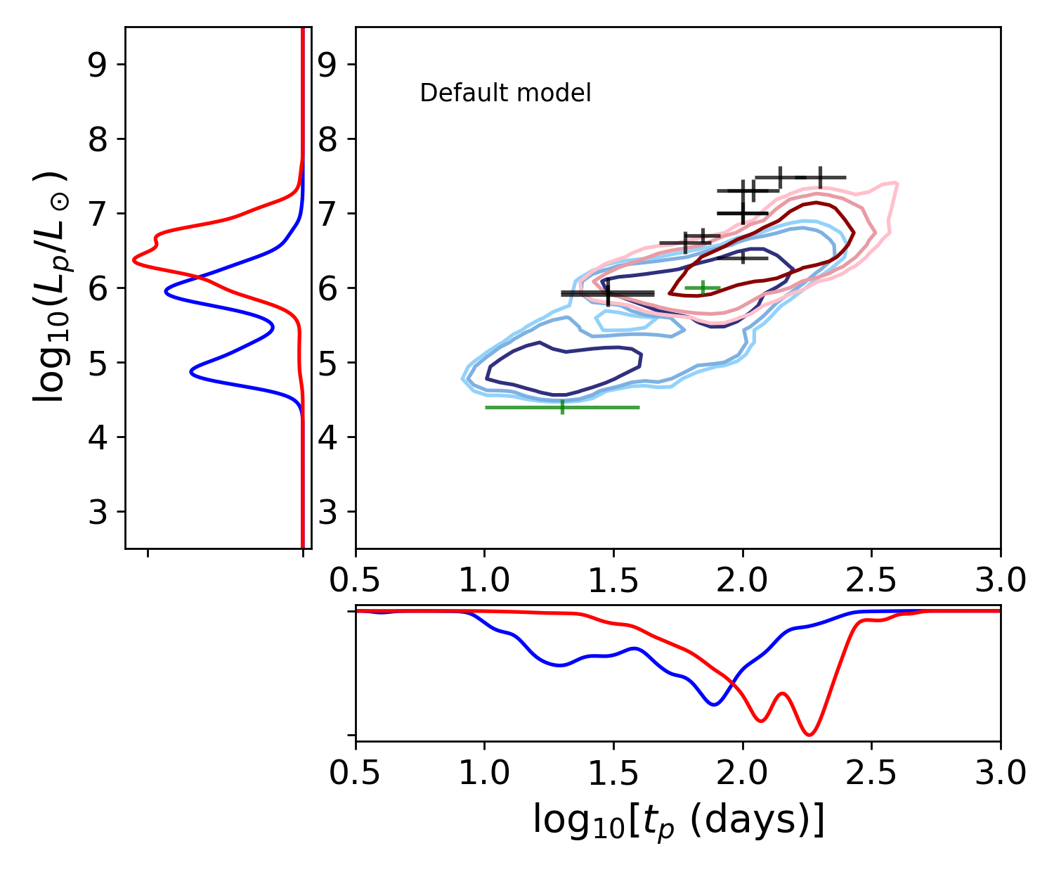
Figure 1: Predicted joint luminosity/duration distribution of luminous red nova plateaux using the default model. Blue contours show the joint distribution for the intrinsic population in our population synthesis simulation. Red contours show the predicted joint distribution that will be observed by LSST. Contours enclose 68%, 90% and 95% of the total integrated probability. Blue and red curves in the margins are the corresponding one-dimensional distributions. The crosses (line lengths represent uncertainties) show the observed LRNe which occurred inside (green) and outside (black) the Galaxy.

Figure 1 shows that the intrinsic distribution is bimodal, with the two peaks corresponding to dimmer, shorter-duration LRNe from mergers, and brighter, longer-duration LRNe from common-envelope ejections. The selection-biased distribution is dominated by the tail of the brightest events from ejections. The majority of the LRNe in table 1 are, within error, inside the outermost contour, however the five brightest events – NGC 4490–2011OT1, AT 2017jfs, UGC 12307–2013OT1, SNHunt248 and AT 2018hso – are outside the 95% contour. The results for each set of variations are shown in figures 2, 3, and 4.

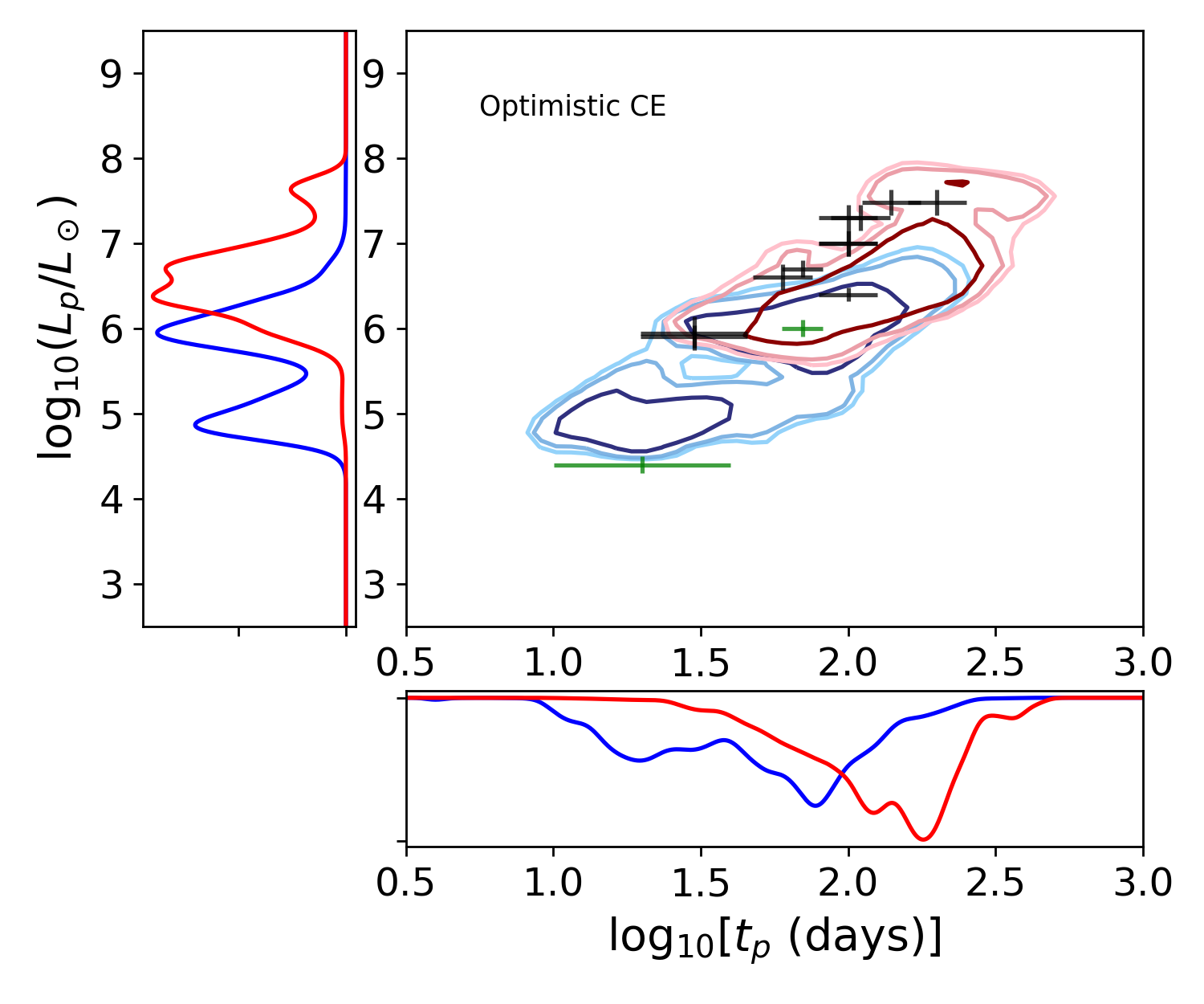
Figure 2: Predicted joint luminosity/duration distribution of luminous red nova plateaux. The contours and symbols have the same meaning as in Figure 1. This plot uses the same default ejecta energy model (i) as Figure 1, but with the optimistic CE assumption.

The optimistic CE assumption (figure 2) produces a plateau distribution with brighter events than the pessimistic CE assumption: an additional peak appears at $\log(L_{p}/L_{\odot})\approx 7.5$. CE events can be initiated by HG donors when the binary is more compact and the envelope is more tightly bound than for more evolved donors; in our ejecta energy model, this leads to brighter LRNe. Only the optimistic CE assumption predicts a distribution which includes the brightest LRNe with the default energy prescription (i).

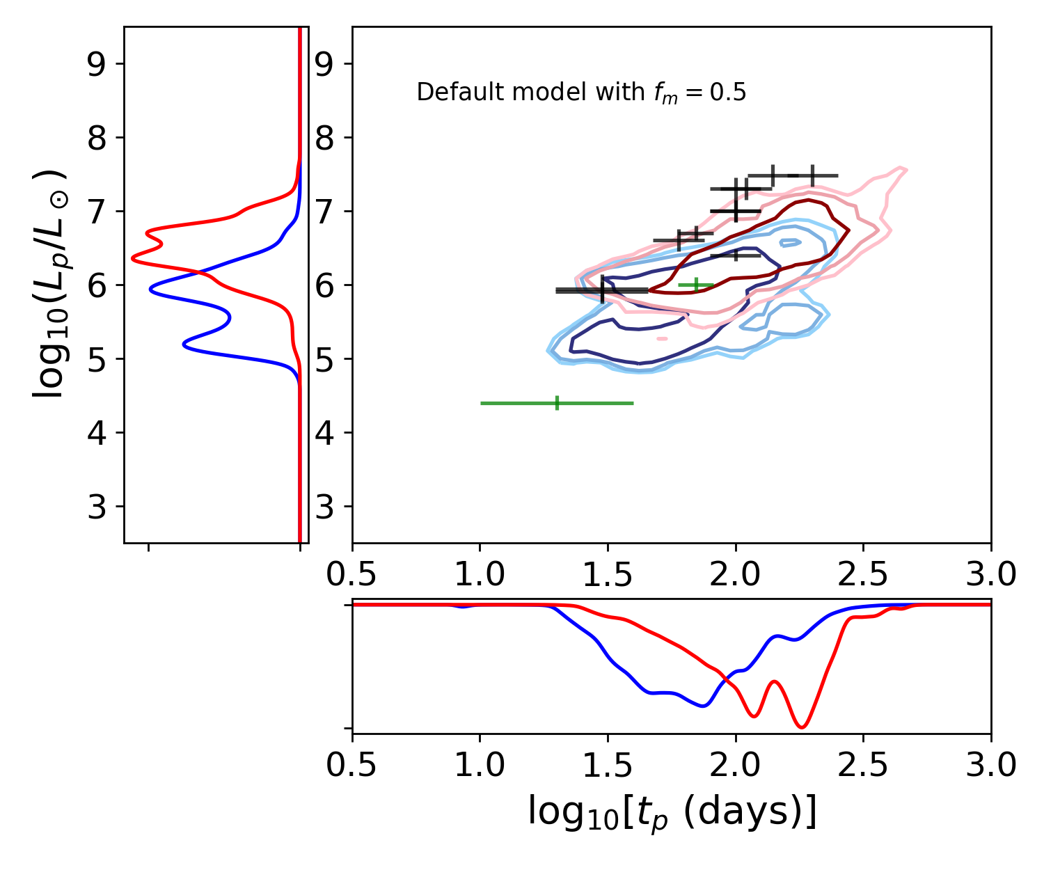
Figure 3: Predicted joint luminosity/duration distribution of luminous red nova plateaux. The contours and symbols have the same meaning as in Figure 1. This plot uses the same default ejecta energy model (i) as Figure 1, but with the merger ejection fraction set to$f_{\mathrm{m}}=0.5$.

Figure 3 shows that the mass fraction ejected during mergers does not substantially change the selection-biased distributions, which are dominated by common-envelope ejections. Increasing the mass fraction ejected during mergers does bring the two peaks representing mergers and ejections closer together in the intrinsic luminosity distribution (blue curve), which leads to a poorer match between predictions and the observed Galactic LRNe. In particular, V1309 Sco lies outside the 95% integrated probability density contour.

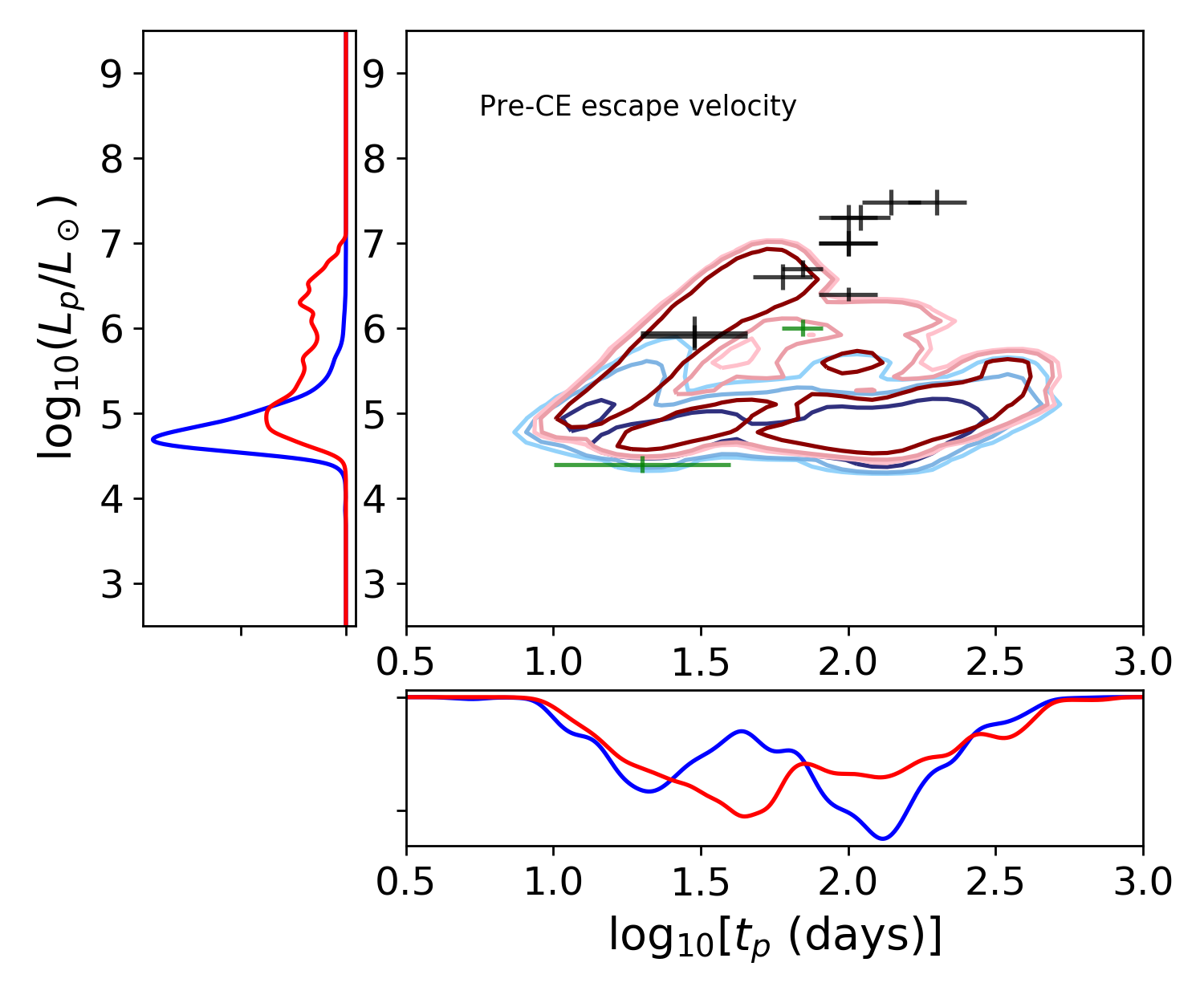
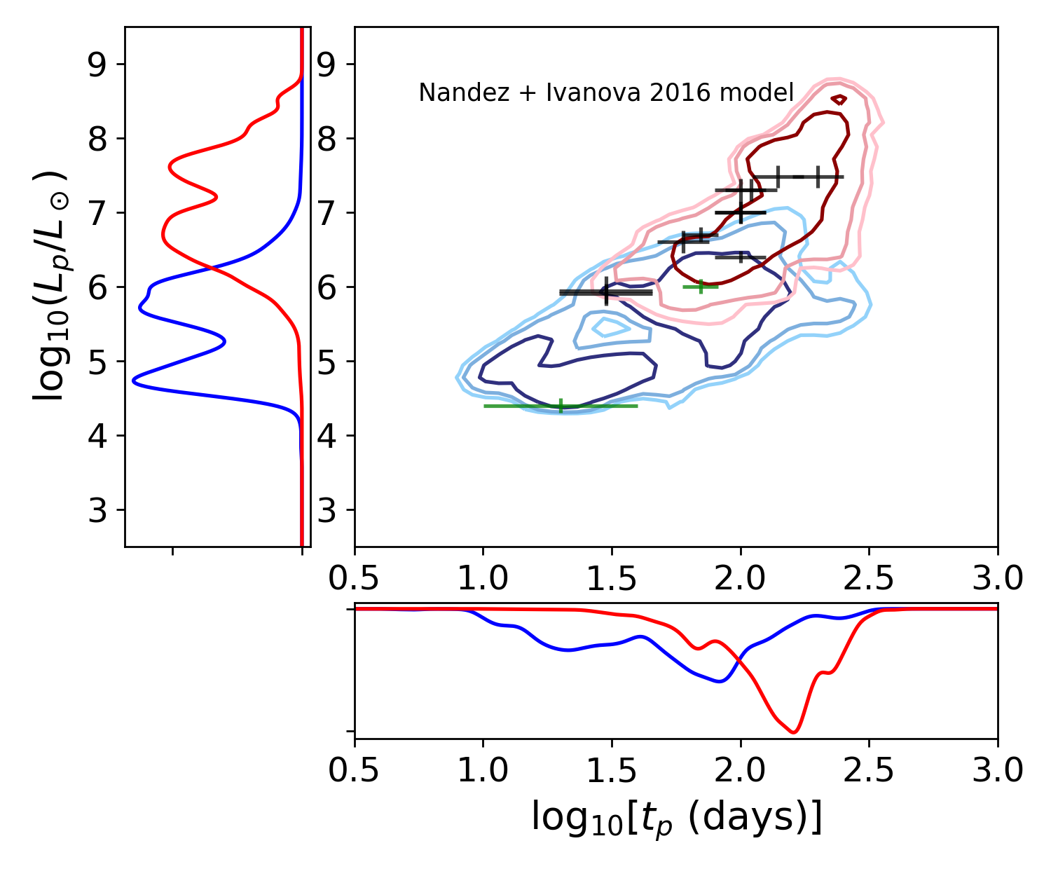
Figure 4: Predicted joint luminosity/duration distributions of luminous red nova plateaux. The contours and symbols have the same meaning as in Figure 1. The panels show predictions for different prescriptions for the ejecta energy $E_{\mathrm{k}}^{\infty}$: pre-CE escape velocity prescription (ii-a) in the top panel, post-CE escape velocity prescription (ii-b) in the middle panel, Nandez & Ivanova (2016) prescription (iii) in the bottom panel.

Figure 4 shows that the choice of model for the ejecta energy $E_{\mathrm{k}}^{\infty}$ significantly affects our predicted distributions. The pre-CE escape velocity $E_{\mathrm{k}}^{\infty}$ prescription (ii-a) has a unimodal luminosity distribution with reduced ejection energies and yields a significant density near many of the observed events, but does not produce any LRNe as bright as the five brightest. The reduced ejecta energies in this model deprive the intrinsic distribution of high-luminosity tails, so that the difference between the intrinsic distribution and the luminosity-biased distribution is less pronounced for this model than for other models. On the other hand, the post-CE escape velocity $E_{\mathrm{k}}^{\infty}$ prescription (ii-b) predicts a distribution dominated by brighter, longer duration events than the other models, and has significant density around all observed extragalactic LRNe. Meanwhile, the Nandez & Ivanova (2016) prescription (iii) yields a broad range of plateau durations but generally favours lower luminosities and again does not predict any events as bright as the five brightest observed LRNe.

3.3 Event rates

3.3.1 Galactic

Both the intrinsic rate of common-envelope events and the observed rate of LRN transients are highly uncertain. The best constraint on the rate of LRNe comes from the number detected within the Galaxy, which, given the long duration and brightness of LRNe, we can assume to be close to a complete sample (though see discussion in Kochanek et al., 2014). The detection of three Galactic LRNe within the last 25 years gives a Galactic rate of $\sim 0.12$ yr^-1 per Milky Way equivalent galaxy, or one event per $\sim 17$ M_⊙ of star formation, assuming a Milky Way star formation rate of $2$ M_⊙ yr^-1 (Licquia & Newman, 2015). Ofek et al. (2008) inferred a 95%-confidence lower limit of 0.019 yr^-1 on the rate based on the observations of V838 Mon and V4332 Sgr. These values match the rate from our simulation of one event per $19.1M_{\odot}$ of star formation, or 0.1 yr^-1 in the Milky Way. They also roughly agree with a previous population study by Kochanek et al. (2014), who modelled the Galactic rate of common-envelope events to be 0.2 yr^-1.

In Figure 5 we show the intrinsic (i.e. Galactic) rate of LRNe as a function of absolute magnitude $(m)$ predicted by our default model. We also show the observational upper limit constraints from Adams et al. (2018) as the grey shaded region, and the empirical constraints from Kochanek et al. (2014) as the green shaded region. Our model agrees with both constraints, except for the brightest events with $M\lesssim-12$, where it diverges from the rate of Kochanek et al. (2014). However, their rate is derived from only three Galactic observations, and is extrapolated for bright events.

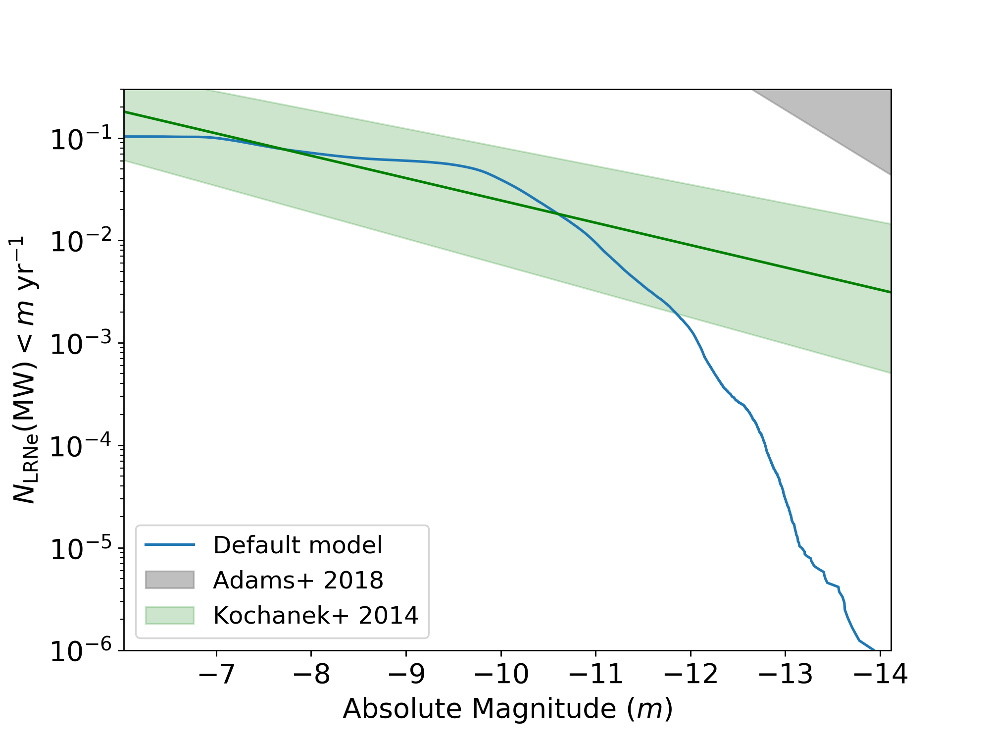
Figure 5: Rate of Galactic LRNe brighter than a given absolute magnitude $m$ as predicted by our default model. The gray shaded region corresponds to the observational upper limit from Adams et al. (2018), and the green line and shaded region correspond to empirical constraints from Galactic LRNe in Kochanek et al. (2014). Note that the comparison is not exact, as our magnitudes are bolometric while those of Adams et al. (2018) and Kochanek et al. (2014) are in the $I$ band.

3.3.2 Extragalactic

Outside the Galaxy, assuming a star formation rate of $0.015$ $M_{\odot}$ Mpc^-3 yr^-1 (Madau & Dickinson, 2014), our predicted local average LRN rate is $\sim 8\times 10^{-4}$ Mpc^-3 yr^-1. Comparing our volumetric LRN rate with the rate of formation of binary black holes which merge within a Hubble time, 24–112 Gpc^-3 yr^-1 (Abbott et al., 2019), we predict that LRNe are $\sim 10^{4}$ times more common than the formation of merging BBHs, and hence, even if the majority of BBHs are formed through common-envelope evolution, their progenitors are unlikely to form an appreciable sub-population of LRNe.

3.3.3 Upcoming surveys - LSST and ZTF

We make predictions for the populations of LRNe observable in future surveys with LSST (LSST Science Collaboration et al., 2009) and the Zwicky Transient Facility (ZTF) (Graham et al., 2019; Bellm et al., 2019).

In the top panel of Figure 6 we show the predicted detection rate for LRNe with LSST as a function of plateau luminosity for the model variants described in section 2.4. The bottom panel of Figure 6 shows the same for ZTF.

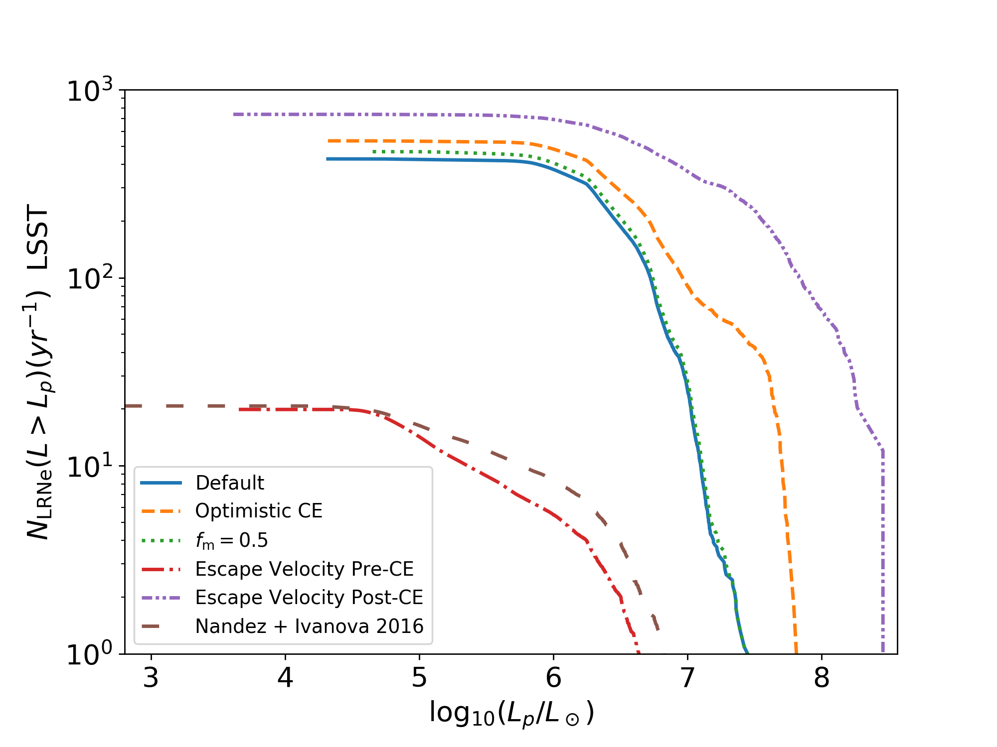
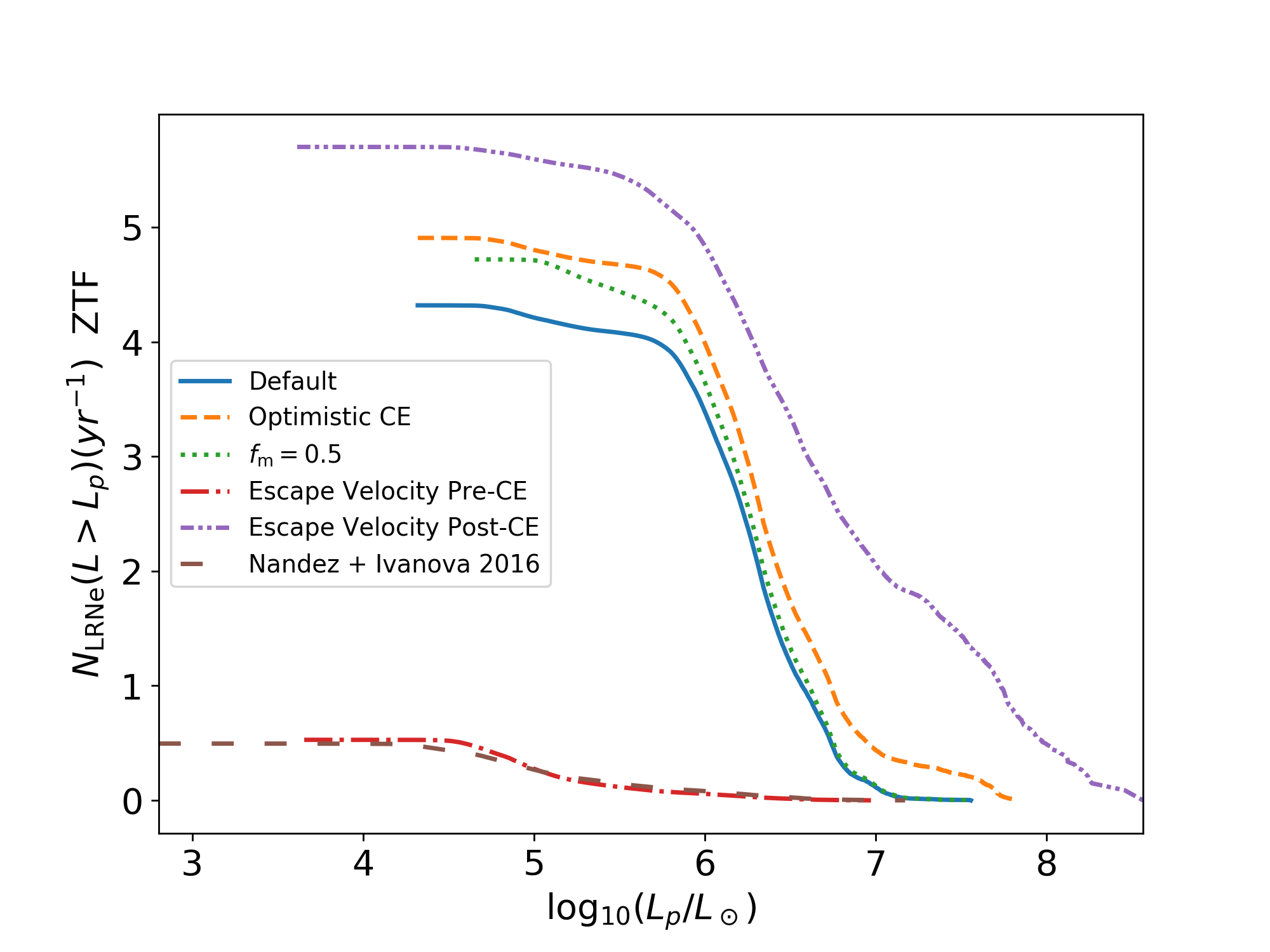
Figure 6: Top panel: cumulative rate of LRNe observed by LSST brighter than a given plateau luminosity $L_{p}$ as predicted by our default model and model variations described in section 2.4. Bottom panel: cumulative rate of LRNe observed by ZTF (while the scaling between curves corresponding to different models is the same as in the top panel, but vertical axis is linear rather than logarithmic for clarity) .

The default model predicts 430 LRN detections per year with LSST, and we summarise the rates from our model variations in Table 2.

Model Name	LSST Rate	ZTF Rate
	[yr-1]	[yr-1]
Default	430	4.3
Optimistic CE	530	4.9
$f_{\mathrm{m}}=0.5$	470	4.7
(ii-a) Pre-CE escape velocity	20	0.5
(ii-b) Post-CE escape velocity	740	5.7
(iii) Nandez & Ivanova 2016	20	0.5

Table 2: Predicted LRN detection rates with LSST and ZTF for the models we consider in this work.

Apart from the pre-CE escape velocity model (ii-a) and the Nandez & Ivanova (2016) model (iii(), all our LSST detection rate estimates fall within the previously predicted LSST detection rate envelope of 80–3400 yr^-1 (LSST Science Collaboration et al., 2009). With our default model, we predict that ZTF will detect $\approx 4$ LRN each year, consistent with Adams et al. (2018), and between our various models we predict between $\approx 0.5$–$6$ LRNe per year with ZTF.

We find that the brightest LRNe have luminosities $6.5<\log_{10}(L_{p}/L_{\odot})<8.5$ (absolute bolometric magnitudes $-11.5>m>-16.5$), depending on our model assumptions. The brightest observed LRN NGC4490-OT (Smith et al., 2016; Pastorello et al., 2019) had an absolute bolometric magnitude of $\sim-14$, suggesting it was among the brightest such events we can expect to observe.

4 Discussion

We have considered a range of models for connecting CE events to LRNe, although this is not an exhaustive list of plausible variations. The current sample of observed Galactic and extragalactic LRNe is already constraining. Only our default ejecta energy model (i) with optimistic CE and the post-CE escape velocity ejecta energy model (ii-b) can plausibly explain all events. The rest of our models fail to predict LRNe as bright as NGC 4490–2011OT1, AT 2017jfs, UGC 12307–2013OT1, SNHunt248 and AT 2018hso; and, in the case of the default model with $f_{\mathrm{m}}=0.5$, fail to predict LRNe as dim as V1309 Sco. Of course, we only consider a limited set of plausible variations for LRN energetics and common-envelope physics. Our goal is not to tweak the models in order to match the observations (which is possible, but uninformative), but rather to explore the range of predicted detection rates and the science that can be done with a growing data set.

Our plausible models predict LRN detection rates with LSST of roughly 500 detections per year, in line with previous predictions, and LRN detection rates of roughly 5 per year with ZTF. We also predict a pronounced difference between the intrinsic population of LRNe plateaux and the observed population. The intrinsic population has roughly similar amounts of LRNe from mergers and common-envelope ejections, which results in a bimodal plateau luminosity distribution. The extragalactic selection-biased population, however, is dominated by the brightest events, which are almost exclusively due to envelope ejections.

In determining the observed rate of LRNe, we ignored the time delay between star formation and the common envelope event. Since our model for the Milky Way assumes a constant star formation rate and metallicity, this time delay does not affect our predictions for the population of LRNe observable in the Galaxy.

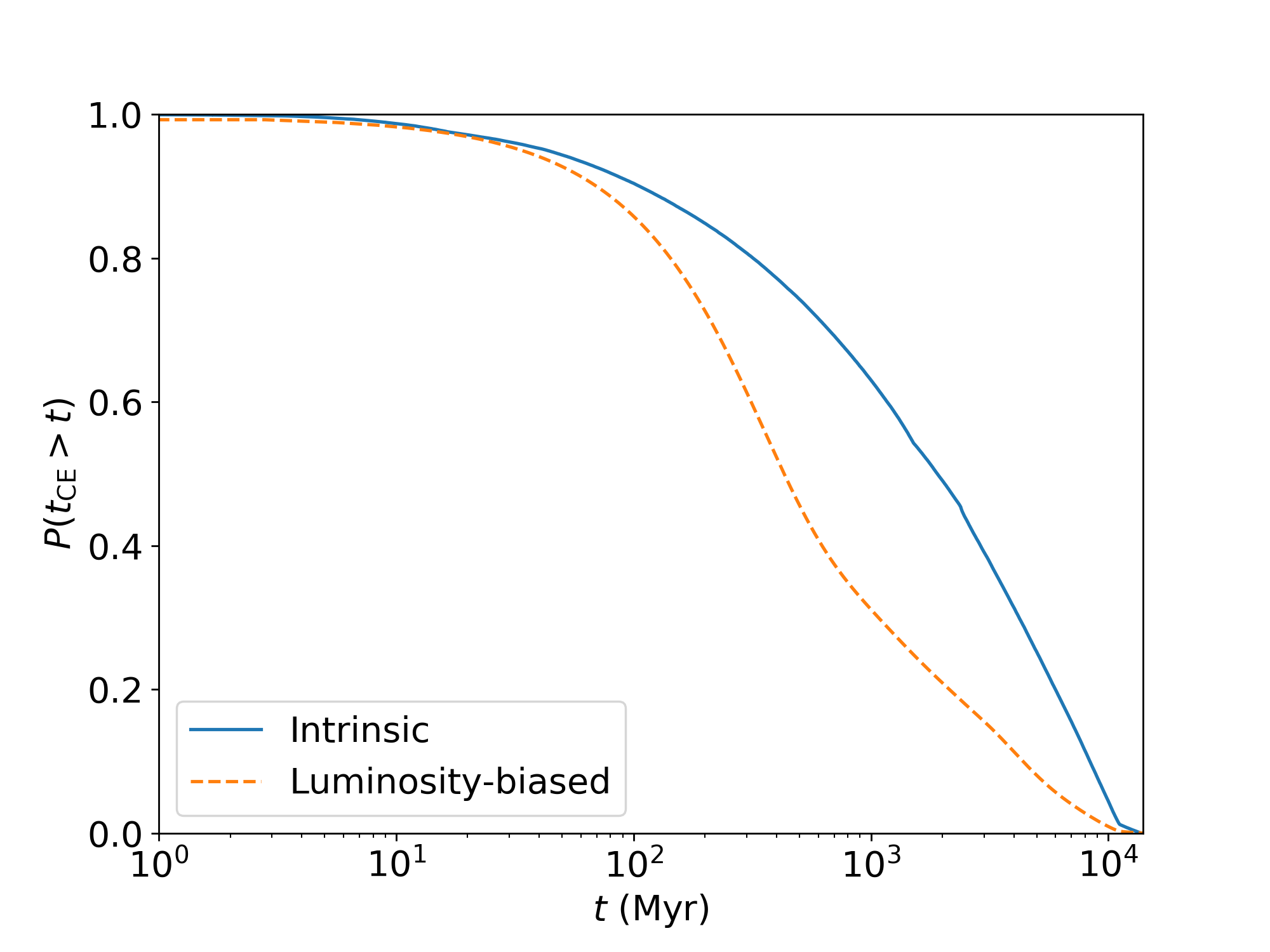
Figure 7: Cumulative distribution of the delay time between star formation and CE event. The blue solid curve shows the intrinsic distribution, while the orange dashed curve includes the observational bias.

On the other hand, for extragalactic LRNe, a binary undergoing a common envelope event observable today could have formed up to $\sim 10$ Gyr ago (see Figure 7), corresponding to a redshift of $z\approx 2$, when the global star formation rate was a factor $\sim 10$ higher (Madau & Dickinson, 2014). However, this long tail of the delay-time distribution is due to low-mass stars, which typically produce dim LRNe. This can be understood analytically as follows. The masses of stars are distributed according to the IMF, which for the masses we consider, $M>1$ M_⊙, scales as $M^{-2.3}$ (Salpeter, 1955; Kroupa, 2001), with low mass stars being the most common (see Figure 8). The lifetime of a low mass star scales with its mass as $t\sim M^{-2.5}$. The distribution of main sequence lifetimes thus scales as $\mathrm{d}N/\mathrm{d}t\sim t^{-0.5}$ with a median delay time of $\sim 2$ Gyr. Moreover, the brightest, luminosity-selected events are dominated by more massive, rapidly evolving stars (see Figure 8). Consequently, the luminosity-selected events have median delay times of well under a Gyr, as shown in Figure 7. Since the cosmic star formation rate did not change significantly on this timescale (Madau & Dickinson, 2014), we can use the simplifying assumption of a constant star formation rate throughout. On the other hand, variations in the metallicity of star-forming gas (Madau & Dickinson, 2014; Neijssel et al., 2019; Chruslinska & Nelemans, 2019) are potentially important, and have not been addressed here.

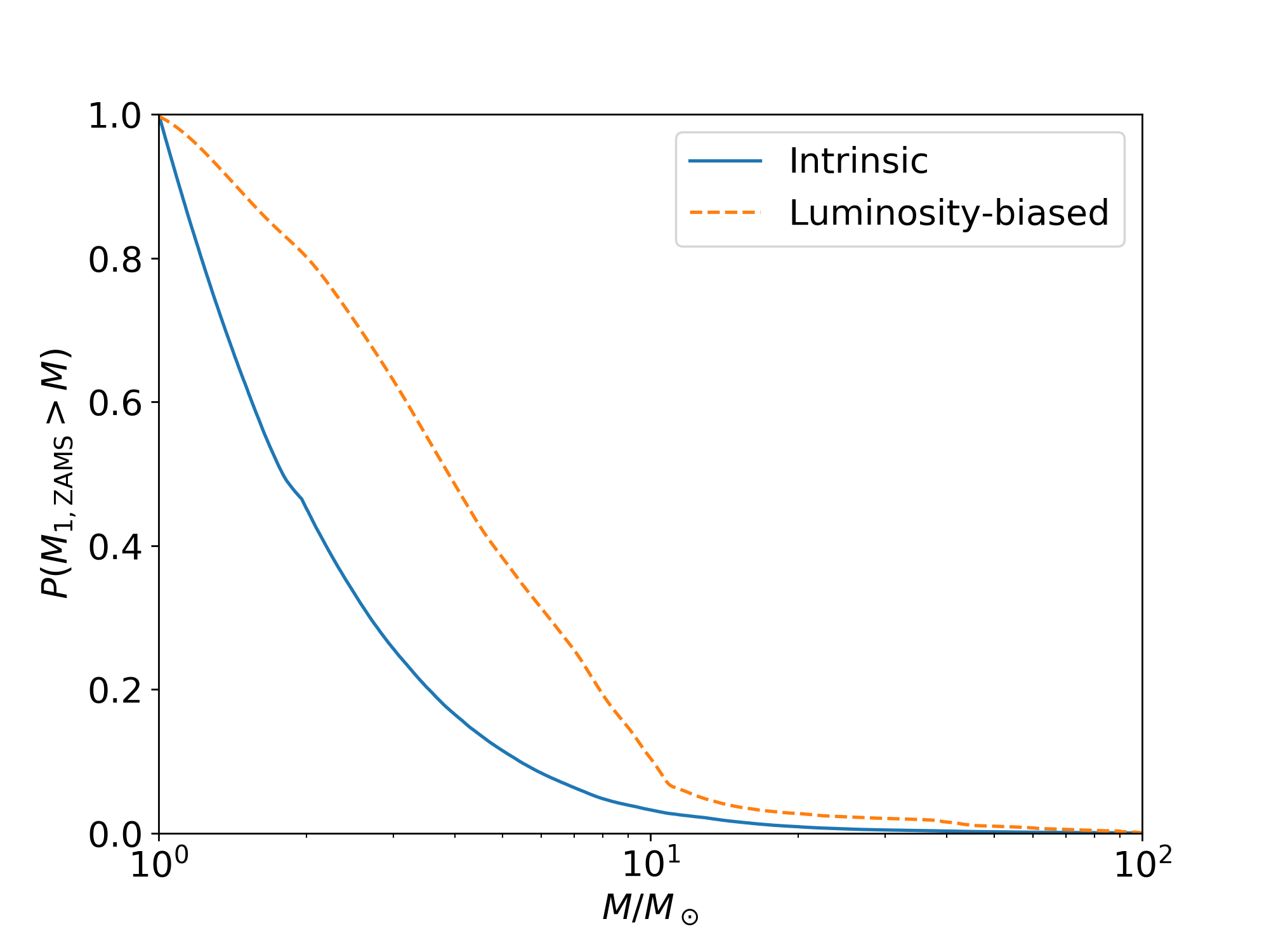
Figure 8: Cumulative distribution of the birth mass of the initially more massive star $m_{1}$ in our default model. The blue solid curve shows the intrinsic distribution, while the orange dashed curve includes the selection bias.

For simplicity, we have assumed that all stars form in binaries in our models, although only around $\sim 50\%$ of these binaries interact (exchange mass) at some point during their lives. Observations have shown that stellar multiplicity appears to be a function of stellar mass. The majority of massive stars are born in binaries (e.g. Sana et al., 2012; Moe & Di Stefano, 2017), but the fraction of stars with companions decreases for lower-mass stars (Raghavan et al., 2010). Since the majority of luminosity-selected LRNe arise from binaries with $M_{\mathrm{1\,ZAMS}}>4\,M_{\odot}$ stars (see Figure 8), neglecting this trend introduces an uncertainty in quoted event rates that is well below other sources of modelling uncertainty.

Another caveat is the possibility that some of the bright, long-duration events predicted here will be self-obscured by the optically thick ejecta, and will be re-processed into the infrared (c.f. Minniti et al., 2017; Kasliwal et al., 2017; Oskinova et al., 2018). Of course, the existence of very bright LRNe such as NGC 4490-OT2011 (Smith et al., 2016) would argue that at least some LRNe avoid this fate. However, NGC 4490-OT2011 appears to resemble SN 2008S (Arbour & Boles, 2008), which is not a consensus LRN candidate.

Clayton et al. (2017) argued that some common envelope events may have multiple ejections. This would increase the rates relative to those we quote, but could decrease the luminosity and duration of individual LRNe, especially if later ejections are obscured by the material emitted during earlier ones.

Massive red supergiants (RSGs) in low-metallicity environments have been invoked to explain the formation through common-envelope evolution (e.g. Belczynski et al., 2016; Stevenson et al., 2017, 2019) of the merging binary black holes being observed by Advanced LIGO and Virgo (Abbott et al., 2019). However, there are no massive RSGs observed in the Milky Way and the Magellanic Clouds with a luminosity greater than $\sim 10^{5.5}$ L_⊙ (Humphreys & Davidson, 1979; Levesque, 2017). Stellar models predict that the most massive RSGs correspond to single stars with initial masses of $\sim 40$ M_⊙ (e.g. Ekström et al., 2012; Sanyal et al., 2017; Groh et al., 2019). In our model, stars with initial masses $\gtrsim 40$ M_⊙ have high mass loss rates and do not form RSGs at solar metallicity.

Using our model, we can estimate what the luminosity of a LRN with a massive RSG donor would look like. Taking approximate sample parameters of a $40M_{\odot}$, $10^{5.4}L_{\odot}$ donor with a temperature of $4000$ K and hence a radius of $\sim 1000R_{\odot}$ which ejects a 20 $M_{\odot}$ envelope during a CE event would yield a $1.3\times 10^{7}L_{\odot}$ LRN according to the default ejecta energy prescription (i). This lies at the upper end of our predictions using this model, and suggests that a population of more luminous events with red progenitors would point to the existence of massive RSGs. RSGs can have higher masses and smaller radii for a given mass at lower metallicity. The plateau luminosity scales as donor radius to the $-1/6$ power in model (i) if all other properties remain unchanged, and as mass to the $7/6$ power, so LRNe with massive RSG donors would be brighter in low-metallicity environments. However, alternative models, such as the post-CE energy ejecta model (ii-b), predict events of this luminosity from COMPAS populations that do not have massive RSGs, consistent with the $3\times 10^{7}L_{\odot}$ LRN NGC 4490-OT2011 that is associated with a blue progenitor.

Observations of the significant population of LRNe that will be accessible with LSST will provide insights on CE physics and the evolution of massive stars that will be complementary to existing observations. Given the critical importance of CE events to massive binary evolution, LRNe may play an important role in elucidating massive binaries as progenitors of gravitational-wave sources.

References

- Abbott et al. (2019) Abbott B. P., et al., 2019, Physical Review X, 9, 031040
- Abt (1983) Abt H. A., 1983, ARA&A, 21, 343
- Adams et al. (2016) Adams S. M., Kochanek C. S., Prieto J. L., Dai X., Shappee B. J., Stanek K. Z., 2016, Mon. Not. Roy. Astron. Soc., 460, 1645
- Adams et al. (2018) Adams S. M., et al., 2018, PASP, 130, 034202
- Arbour & Boles (2008) Arbour R., Boles T., 2008, Central Bureau Electronic Telegrams, 1234
- Asplund et al. (2009) Asplund M., Grevesse N., Sauval A. J., Scott P., 2009, ARA&A, 47, 481
- Banerjee et al. (2018) Banerjee D. P. K., et al., 2018, ApJ, 867, 99
- Barrett et al. (2018) Barrett J. W., Gaebel S. M., Neijssel C. J., Vigna-Gómez A., Stevenson S., Berry C. P. L., Farr W. M., Mandel I., 2018, MNRAS, 477, 4685
- Belczynski et al. (2007) Belczynski K., Kalogera V., Rasio F. A., Taam R. E., Bulik T., 2007, Astrophys. J., 662, 504
- Belczynski et al. (2016) Belczynski K., Holz D. E., Bulik T., O’Shaughnessy R., 2016, Nature, 534, 512
- Bellm et al. (2019) Bellm E. C., et al., 2019, PASP, 131, 018002
- Berger et al. (2009) Berger E., et al., 2009, ApJ, 699, 1850
- Blagorodnova et al. (2017) Blagorodnova N., et al., 2017, ApJ, 834, 107
- Bond et al. (2009) Bond H. E., Bedin L. R., Bonanos A. Z., Humphreys R. M., Monard L. A. G. B., Prieto J. L., Walter F. M., 2009, ApJ, 695, L154
- Cai et al. (2019) Cai Y. Z., et al., 2019, A&A, 632, L6
- Chruslinska & Nelemans (2019) Chruslinska M., Nelemans G., 2019, MNRAS, 488, 5300
- Clayton et al. (2017) Clayton M., Podsiadlowski P., Ivanova N., Justham S., 2017, MNRAS, 470, 1788
- De Marco et al. (2011) De Marco O., Passy J.-C., Moe M., Herwig F., Mac Low M.-M., Paxton B., 2011, MNRAS, 411, 2277
- Dewi & Tauris (2000) Dewi J. D. M., Tauris T. M., 2000, Astron. Astrophys., 360, 1043
- Dominik et al. (2012) Dominik M., Belczynski K., Fryer C., Holz D., Berti E., Bulik T., Mandel I., O’Shaughnessy R., 2012, Astrophys. J., 759, 52
- Eggleton (1983) Eggleton P. P., 1983, ApJ, 268, 368
- Ekström et al. (2012) Ekström S., et al., 2012, A&A, 537, A146
- Farr et al. (2015) Farr W. M., Gair J. R., Mandel I., Cutler C., 2015, Phys. Rev. D, 91, 023005
- Ge et al. (2015) Ge H., Webbink R. F., Chen X., Han Z., 2015, ApJ, 812, 40
- Glebbeek et al. (2013) Glebbeek E., Gaburov E., Portegies Zwart S., Pols O. R., 2013, MNRAS, 434, 3497
- Goranskij et al. (2016) Goranskij V. P., et al., 2016, Astrophysical Bulletin, 71, 82
- Graham et al. (2019) Graham M. J., et al., 2019, PASP, 131, 078001
- Groh et al. (2019) Groh J. H., et al., 2019, A&A, 627, A24
- Hayashi & Nakano (1963) Hayashi C., Nakano T., 1963, Progress of Theoretical Physics, 30, 460
- Hjellming & Webbink (1987) Hjellming M. S., Webbink R. F., 1987, ApJ, 318, 794
- Humphreys & Davidson (1979) Humphreys R. M., Davidson K., 1979, ApJ, 232, 409
- Hurley et al. (2000) Hurley J. R., Pols O. R., Tout C. A., 2000, MNRAS, 315, 543
- Iaconi & De Marco (2019) Iaconi R., De Marco O., 2019, MNRAS, 490, 2550
- Iben & Tutukov (1984) Iben Jr. I., Tutukov A. V., 1984, Astrophys. J. Suppl., 54, 335
- Ivanova (2011) Ivanova N., 2011, ApJ, 730, 76
- Ivanova & Chaichenets (2011) Ivanova N., Chaichenets S., 2011, ApJ, 731, L36
- Ivanova et al. (2013a) Ivanova N., et al., 2013a, A&ARv, 21, 59
- Ivanova et al. (2013b) Ivanova N., Justham S., Nandez J. L. A., Lombardi Jr J. C., 2013b, Science, 339, 433
- Jencson et al. (2019) Jencson J. E., et al., 2019, ApJ, 880, L20
- Kamiński et al. (2015) Kamiński T., Menten K. M., Tylenda R., Hajduk M., Patel N. A., Kraus A., 2015, Nature, 520, 322
- Kankare et al. (2015) Kankare E., et al., 2015, A&A, 581, L4
- Kasen & Woosley (2009) Kasen D., Woosley S. E., 2009, ApJ, 703, 2205
- Kasliwal et al. (2011) Kasliwal M. M., et al., 2011, ApJ, 730, 134
- Kasliwal et al. (2017) Kasliwal M. M., et al., 2017, Astrophys. J., 839, 88
- Kimeswenger (2006) Kimeswenger S., 2006, Astron. Nachr., 327, 44
- Klencki et al. (2018) Klencki J., Moe M., Gladysz W., Chruslinska M., Holz D. E., Belczynski K., 2018, A&A, 619, A77
- Kochanek et al. (2014) Kochanek C. S., Adams S. M., Belczynski K., 2014, MNRAS, 443, 1319
- Kroupa (2001) Kroupa P., 2001, Mon. Not. Roy. Astron. Soc., 322, 231
- Kruckow et al. (2016) Kruckow M. U., Tauris T. M., Langer N., Szécsi D., Marchant P., Podsiadlowski P., 2016, Astron. Astrophys., 596, A58
- Kulkarni et al. (2007) Kulkarni S. R., et al., 2007, Nature, 447, 458
- Kulkarni et al. (2018) Kulkarni S. R., Perley D. A., Miller A. A., 2018, ApJ, 860, 22
- Kumar (1963) Kumar S. S., 1963, ApJ, 137, 1121
- Kurtenkov et al. (2015) Kurtenkov A. A., et al., 2015, A&A, 578, L10
- LSST Science Collaboration et al. (2009) LSST Science Collaboration et al., 2009, preprint, (arXiv:0912.0201)
- LSST Science Collaboration et al. (2017) LSST Science Collaboration et al., 2017, arXiv e-prints, p. arXiv:1708.04058
- Levesque (2017) Levesque E. M., 2017, Astrophysics of Red Supergiants, doi:10.1088/978-0-7503-1329-2.
- Licquia & Newman (2015) Licquia T. C., Newman J. A., 2015, ApJ, 806, 96
- Licquia et al. (2015) Licquia T. C., Newman J. A., Brinchmann J., 2015, ApJ, 809, 96
- Lipunov et al. (2017) Lipunov V. M., et al., 2017, MNRAS, 470, 2339
- Lombardi et al. (2002) Lombardi Jr. J. C., Warren J. S., Rasio F. A., Sills A., Warren A. R., 2002, ApJ, 568, 939
- Loveridge et al. (2011) Loveridge A. J., van der Sluys M. V., Kalogera V., 2011, ApJ, 743, 49
- MacLeod et al. (2017) MacLeod M., Macias P., Ramirez-Ruiz E., Grindlay J., Batta A., Montes G., 2017, ApJ, 835, 282
- Madau & Dickinson (2014) Madau P., Dickinson M., 2014, ARA&A, 52, 415
- Martini et al. (1999) Martini P., Wagner R. M., Tomaney A., Rich R. M., della Valle M., Hauschildt P. H., 1999, AJ, 118, 1034
- Mauerhan et al. (2018) Mauerhan J. C., Van Dyk S. D., Johansson J., Fox O. D., Filippenko A. V., Graham M. L., 2018, MNRAS, 473, 3765
- Metzger & Pejcha (2017) Metzger B. D., Pejcha O., 2017, MNRAS, 471, 3200
- Miller & Scalo (1979) Miller G. E., Scalo J. M., 1979, ApJS, 41, 513
- Minniti et al. (2017) Minniti D., et al., 2017, ApJ, 849, L23
- Moe & Di Stefano (2017) Moe M., Di Stefano R., 2017, The Astrophysical Journal Supplement Series, 230, 15
- Mould et al. (1990) Mould J., et al., 1990, ApJ, 353, L35
- Nandez & Ivanova (2016) Nandez J. L. A., Ivanova N., 2016, MNRAS, 460, 3992
- Nandez et al. (2014) Nandez J. L. A., Ivanova N., Lombardi Jr. J. C., 2014, ApJ, 786, 39
- Nariai & Sugimoto (1976) Nariai K., Sugimoto D., 1976, PASJ, 28, 593
- Neijssel et al. (2019) Neijssel C. J., et al., 2019, MNRAS, 490, 3740
- Ofek et al. (2008) Ofek E. O., et al., 2008, Astrophys. J., 674, 447
- Oskinova et al. (2018) Oskinova L. M., Bulik T., Gómez-Morán A. N., 2018, A&A, 613, L10
- Paczynski (1976) Paczynski B., 1976, in Eggleton P., Mitton S., Whelan J., eds, IAU Symposium Vol. 73, Structure and Evolution of Close Binary Systems. p. 75
- Pastorello et al. (2007) Pastorello A., et al., 2007, Nature, 449, E1
- Pastorello et al. (2019) Pastorello A., et al., 2019, A&A, 630, A75
- Pavlovskii et al. (2017) Pavlovskii K., Ivanova N., Belczynski K., Van K. X., 2017, MNRAS, 465, 2092
- Politano et al. (2010) Politano M., van der Sluys M., Taam R. E., Willems B., 2010, ApJ, 720, 1752
- Popov (1993) Popov D. V., 1993, ApJ, 414, 712
- Prieto et al. (2008) Prieto J. L., et al., 2008, ApJ, 681, L9
- Prieto et al. (2009) Prieto J. L., Sellgren K., Thompson T. A., Kochanek C. S., 2009, ApJ, 705, 1425
- Raghavan et al. (2010) Raghavan D., et al., 2010, The Astrophysical Journal Supplement Series, 190, 1
- Rau et al. (2007) Rau A., Kulkarni S. R., Ofek E. O., Yan L., 2007, Astrophys. J., 659, 1536
- Salpeter (1955) Salpeter E. E., 1955, ApJ, 121, 161
- Sana et al. (2012) Sana H., et al., 2012, Science, 337, 444
- Sanyal et al. (2017) Sanyal D., Langer N., Szécsi D., -C Yoon S., Grassitelli L., 2017, A&A, 597, A71
- Schrøder et al. (2019) Schrøder S. L., MacLeod M., Loeb A., Vigna-Gómez A., Mandel I., 2019, arXiv e-prints, p. arXiv:1906.04189
- Scott (1992) Scott D., 1992, Multivariate Density Estimation: Theory, Practice, and Visualization. A Wiley-interscience publication, Wiley, https://books.google.com.au/books?id=7crCUS_F2ocC
- Segev et al. (2019) Segev R., Sabach E., Soker N., 2019, ApJ, 884, 58
- Smarr & Blandford (1976) Smarr L. L., Blandford R., 1976, ApJ, 207, 574
- Smith et al. (2016) Smith N., et al., 2016, Mon. Not. Roy. Astron. Soc., 458, 950
- Soberman et al. (1997) Soberman G. E., Phinney E. S., van den Heuvel E. P. J., 1997, A&A, 327, 620
- Soker & Tylenda (2003) Soker N., Tylenda R., 2003, ApJ, 582, L105
- Stevenson et al. (2017) Stevenson S., Vigna-Gómez A., Mandel I., Barrett J. W., Neijssel C. J., Perkins D., de Mink S. E., 2017, Nature Communications, 8, 14906
- Stevenson et al. (2019) Stevenson S., Sampson M., Powell J., Vigna-Gómez A., Neijssel C. J., Szécsi D., Mandel I., 2019, ApJ, 882, 121
- Tauris & Dewi (2001) Tauris T. M., Dewi J. D. M., 2001, Astron. Astrophys., 369, 170
- Tout et al. (1997) Tout C. A., Aarseth S. J., Pols O. R., Eggleton P. P., 1997, MNRAS, 291, 732
- Tutukov & Yungelson (1993) Tutukov A. V., Yungelson L. R., 1993, MNRAS, 260, 675
- Tylenda (2005) Tylenda R., 2005, A&A, 436, 1009
- Tylenda et al. (2011) Tylenda R., et al., 2011, A&A, 528, A114
- Tylenda et al. (2013) Tylenda R., et al., 2013, A&A, 555, A16
- Van Dyk et al. (2000) Van Dyk S. D., Peng C. Y., King J. Y., Filippenko A. V., Treffers R. R., Li W., Richmond M. W., 2000, PASP, 112, 1532
- Vigna-Gómez et al. (2018) Vigna-Gómez A., et al., 2018, MNRAS, 481, 4009
- Voss & Tauris (2003) Voss R., Tauris T. M., 2003, Mon. Not. Roy. Astron. Soc., 342, 1169
- Wang et al. (2016) Wang C., Jia K., Li X.-D., 2016, Research in Astronomy and Astrophysics, 16, 126
- Webbink (1984) Webbink R. F., 1984, Astrophys. J., 277, 355
- Webbink (2008) Webbink R. F., 2008, Common Envelope Evolution Redux. p. 233 (arXiv:0704.0280), doi:10.1007/978-1-4020-6544-6_13
- White et al. (2011) White D. J., Daw E. J., Dhillon V. S., 2011, Classical and Quantum Gravity, 28, 085016
- Williams et al. (2015) Williams S. C., Darnley M. J., Bode M. F., Steele I. A., 2015, ApJ, 805, L18
- Xu & Li (2010a) Xu X.-J., Li X.-D., 2010a, ApJ, 716, 114
- Xu & Li (2010b) Xu X.-J., Li X.-D., 2010b, ApJ, 722, 1985
- de Kool et al. (1987) de Kool M., van den Heuvel E. P. J., Pylyser E., 1987, Astron. Astrophys., 183, 47
- de Mink et al. (2014) de Mink S. E., Sana H., Langer N., Izzard R. G., Schneider F. R. N., 2014, Astrophys. J., 782, 7
- van den Heuvel (1976) van den Heuvel E. P. J., 1976, in Eggleton P., Mitton S., Whelan J., eds, IAU Symposium Vol. 73, Structure and Evolution of Close Binary Systems. p. 35