How the mass of a scalar field influences Resonance Casimir-Polder interaction in Schwarzschild spacetime

Abstract

Resonance Casimir-Polder interaction(RCPI) occurs in nature when one or more atoms are in their excited states and the exchange of real photon is involved between them due to vacuum fluctuations of the quantum fields. In recent times, many attempts have been made to show that the curved spacetime such as the de-Sitter spacetime can be separated from a thermal Minkowski spacetime using RCPI. Motivated from these ideas, here we study the RCPI between two atoms that interact with a massive scalar field in Schwarzschild spacetime provided the atoms are placed in the near-horizon region. Subsequently, we use the tool of the open quantum system and calculate the Lamb shift of the atomic energy level of the entangled states. We show that the behavior of RCPI modifies depending on the mass of the scalar field. In the high mass limit, the interaction becomes short-range and eventually disappears beyond a characteristic length scale of $1/m$, where $m$ is the mass of the scalar field.

I Introduction

The phenomena of Casimir Polder interaction (CPI) occurs between an atom and a conducting plate due to vacuum fluctuation of the quantized fields [1, 2, 3]. It has major applications from the field of quantum electrodynamics (QED) to the signature of gravity [4, 5, 6]. CPI mimics van der Waals force in non-relativistic regime where a dispersive force is acting in few nanometer length scale [7, 8]. In physical chemistry it has also huge implications in atomic adsorption and desorption in the thermally excited surfaces [9]. Experimental realization exists in the case of the motion of Bose-Einstein condensate (BEC) under surface CPI [10]. The other successful efforts have been made to probe more complicated contexts like detecting spacetime curvature [11, 6, 12], Unruh effect [13, 14, 15], Hawking radiation of a black hole and checking thermal and nonthermal scaling in a black hole spacetime [16, 17]. One can show that the background spacetime and the relativistic motion of interacting systems can modify the CPI [13, 14, 15, 11, 6, 12, 17, 16, 18, 19, 20, 21, 22].

CPI generates correlations between multiple quantum systems [23, 24, 25]. Two uncorrelated atom also can be entangled if they both share common environment [26, 27]. Recently Lindblad master equation approach is [28] successfully used to explain the interatomic correlations at Schwarzschild spacetime where vacuum fluctuation of the quantum field takes the vital role to create the entanglement between them. This interatomic correlations are the source of RCPI [6, 29]. Subsequently it has been shown that an uniformly accelerated atom behaves like a system in a thermal bath (Thermalization theorem) [30]. Therefore, RCPI is exactly equal to the second order shift (Lamb shift) [31] due to system-field interaction Hamiltonian [32, 33, 6].

In this paper following the recent works, [6, 29], we theoretically investigate the RCPI between two atoms that interact with a massive scalar field in Schwarzschild spacetime. Two atoms are initially uncorrelated and interact individually with the scalar field. The cross-terms of the two individual system-field coupling Hamiltonian in the second-order of the quantum master equation will give rise to the entanglement between the atoms [27]. Here we show how the interatomic correlations between the atoms depend on the mass of the scalar field by calculating the Lamb shift due to system-field coupling.

We organize the paper in the following way. In section-II we give a general description of open quantum system approach-GKSL (Gorini-Kossakowski-Sudarshan-Lindblad) formalism [34, 35, 36] for the two-atom system then discuss the common environment effect and finally compute the shifts of the energy level of the entangled states due to Lamb shift Hamiltonian. In section- III we review the form of the Schwarzschild metric in the near horizon and find the expression of the two-point correlation function for a massive scalar field. Recently it has been shown that, for Schwarzschild spacetime, beyond a characteristic length scale which is proportional to the inverse of the surface gravity $\kappa$, the RCPI between two entangled atoms is characterized by a $1/L^{2}$ power-law provided the atoms are located close to the horizon [29]. However, the length scale limit beyond the characteristic value is not compatible with the local flatness of the spacetime. A massless scalar field has been considered in the ref. [29] to calculate RCPI. In section-IV we compute RCPI between two atoms that interact with a massive scalar field and point out its dependence on the mass term of the scalar field. Subsequently, we show that the RCPI becomes short-range and eventually disappears beyond a characteristic length scale of $1/m$, $m$ being the mass of the scalar field.

II Dynamics of a two-atom system

We consider a system of two-atom weakly interacts with a common environment but they do not have any mutual interaction. Here we choose the environment to be a quantized massive scalar field. This is a general description of the open quantum system [37], therefore, we follow the formalism of the quantum master equation [31]. The Hamiltonian of the full system can be expressed as,

$$\mathcal{H}=\mathcal{H}_{\text{\tiny S}}^{0}+\mathcal{H}_{\text{\tiny L}}^{0}+\mathcal{H}_{\text{\tiny SL}}~{}.$$ (1)

We assume the atoms have the same Zeeman levels and throughout the paper, we use the natural units, $\hbar=c=1$. The free Hamiltonian of the system can be written as $\mathcal{H}_{\text{\tiny S}}^{0}=\mathcal{H}_{\text{\tiny S}}^{01}+\mathcal{H}_{\text{\tiny S}}^{02}=\frac{1}{2}\omega_{0}\sigma_{3}^{(1)}+\frac{1}{2}\omega_{0}\sigma_{3}^{(2)}$ (The superscript in the Pauli matrices represent the atom number). Here $\sigma_{i}$ are the Pauli matrices, $\omega_{0}$ is the frequency of Zeeman levels and we defined $|g\rangle,|e\rangle$ as the corresponding ground and excited state of the atoms. The free Hamiltonian of the scalar field $\mathcal{H}_{\text{\tiny L}}^{0}$ can be written as [38],

$$\mathcal{H}_{\text{\tiny L}}^{0}=\int\frac{d^{3}k}{(2\pi)^{3}}\omega_{k}a^{\dagger}(k)a(k)~{},$$ (2)

where $\omega_{k}=\sqrt{k^{2}+m^{2}}$, the frequency of the scalar field. Here m is the mass of the scalar field and $a^{\dagger},a$ are the creation and annihilation operator of the quantized field respectively. The coupling Hamiltonian between the atom-scalar field can be defined as [28],

$$\mathcal{H}_{\text{\tiny SL}}=\lambda\sum\limits_{\mu=0}^{3}\big{[}\sigma_{\mu}^{(1)}\otimes\phi(x_{1})+\sigma_{\mu}^{(2)}\otimes\phi(x_{2})\big{]}~{},$$ (3)

where $\lambda$ is the coupling constant and $\phi$ represents the scalar field. Initially, the atoms and the scalar field are separated from each other. Therefore, the initial density matrix can be written as $\rho(0)=\rho_{s}(0)\otimes|0\rangle\langle 0|$ (“Born-Markov” approximation [37]). Here $|0\rangle$ is the vacuum state of the massive scalar field and $\rho_{s}(0)$ is the initial density matrix of the system. For a closed system, “Von-Neumann-Liouville” equation is used to describe the full dynamics,

$$\frac{d\rho(t)}{dt} = -i[\mathcal{H}_{\text{\tiny S}}^{0}+\mathcal{H}_{\text{\tiny L}}^{0}+\mathcal{H}_{\text{\tiny SL}},\rho(t)].$$ (4)

Here, $\rho(t)$ is the total density matrices. Starting from the equation (4) we perturbatively expand the time evolution operator ($U(t,t_{0})=\mathcal{T}\exp\{-i\int^{t}_{t_{0}}dt^{\prime}(\mathcal{H}_{\text{\tiny S}}^{0}+\mathcal{H}_{\text{\tiny L}}^{0}+\mathcal{H}_{\text{\tiny SL}})\}$) to the second order of coupling Hamiltonian [31] and taking trace over field degrees of freedom, we get the quantum master equation, which is also known as GKSL equation [34, 35, 36]. The quantum master equation in the lab-frame with a proper-time $\tau$ can be expressed as [31],

$$\frac{d\rho_{s}(\tau)}{d\tau}=-i[\mathcal{H}_{\text{\tiny S}}^{0}+\mathcal{H}_{lamb},\rho_{s}(\tau)]+\mathcal{L}\big{(}\rho_{s}(\tau)\big{)}~{}.$$ (5)

Here, $\mathcal{H}_{lamb}$ is the Lamb-shift Hamiltonian that leads to the renormalization of Zeeman Hamiltonian and $\mathcal{L}\big{(}\rho_{s}(\tau)\big{)}$ is the dissipator of the master-equation which can be written as [28],

$$\mathcal{L}\big{(}\rho_{s}\big{)} = \sum\limits_{a,b=1}^{2}\sum\limits_{j,k=1}^{3}\gamma^{ab}_{jk}\Big{(}\sigma_{b}^{k}\rho_{s}\sigma_{a}^{j}-\frac{1}{2}\{\sigma_{a}^{j}\sigma_{b}^{k},\rho_{s}\}\Big{)}~{},$$ (6)

$$\mathcal{H}_{lamb} = -\frac{i}{2}\sum\limits_{a,b=1}^{2}\sum\limits_{j,k=1}^{3}\mathcal{S}_{jk}^{ab}\sigma_{a}^{j}\sigma_{b}^{k}~{},$$ (7)

where $\mathcal{S}_{jk}^{ab}$ and $\gamma^{ab}_{jk}$ depend on the Fourier transforms of the two-point correlation functions of the scalar field. The shift terms and dissipative terms are coming from second-order terms of atom-field coupling Hamiltonian and they are Kramer-kronig pair to each-other [37]. As we are interested in the shift between the energy levels of the two-atom system, our main focus is to demonstrate the Lamb-shift term and not to think about decay terms. However, the decay terms are responsible for taking the two-atom system to the equilibrium configuration, which is the Bekenstein-Hawking temperature [30] of the massive scalar field. Lamb shift can be calculated from the Hilbert transforms of the Fourier transforms of the two-point functions which are shown below,

$$\mathcal{K}^{ab}(\omega_{0})=\frac{\mathcal{P}}{\pi i}\int\limits^{\infty}_{-\infty}d\omega\frac{\mathcal{G}^{ab}(\omega)}{\omega-\omega_{0}}~{}.$$ (8)

Here $\mathcal{P}$ denotes the principal value. $\mathcal{G}^{ab}(\omega)$ are the Fourier transforms of the two-point correlation functions of the scalar field. The Fourier transforms of the two-point functions are given by,

$$\mathcal{{G}}^{ab}(\omega) = \int\limits^{\infty}_{-\infty}d\Delta\tau~{}e^{i\omega\Delta\tau}~{}{G}^{ab}(\Delta\tau)~{},$$ (9)

$$\text{where,}\,\,\,\,G^{ab}(\Delta\tau) = \langle{\Phi}(\tau,\mathbf{x}_{a}){\Phi}(\tau^{\prime},\mathbf{x}_{b})\rangle~{},$$ (10)

and $\Delta\tau=(\tau-\tau^{\prime})$. The exact form of $\mathcal{S}^{ab}_{jk}$ can be written as [6],

$$\mathcal{S}^{ab}_{jk}=A^{ab}\delta_{jk}-iB^{ab}\epsilon_{jkl}\delta_{3l}-A^{ab}\delta_{3j}\delta_{3k}~{},$$ (11)

where the terms $A^{ab}$ and $B^{ab}$ are given by,

$$A^{ab} = \frac{\lambda^{2}}{4}\left[\mathcal{K}^{ab}(\omega_{0})+\mathcal{K}^{ab}(-\omega_{0})\right],$$ (12)

$$B^{ab} = \frac{\lambda^{2}}{4}\left[\mathcal{K}^{ab}(\omega_{0})-\mathcal{K}^{ab}(-\omega_{0})\right].$$ (13)

II.1 Entanglement between two atoms through a massive scalar field

Two atoms are initially uncorrelated but due to interaction with the massive scalar field, the energy levels become correlated. So, there is a formation of field-induced entanglement between the atoms which depends on the two-point correlation functions [27]. The two-point functions can be computed along the trajectories of the atoms thus they depend on the spacetime background. Now we aim to calculate the expectation value of $\mathcal{H}_{lamb}$ in the entangled states to investigate the effect of interatomic correlations between two atoms in Schwarzschild spacetime. Here we take the symmetric and anti-symmetric state of the dipolar-coupled Hamiltonian for simplicity because other states are unchanged due to interatomic correlations [39]. The symmetric and anti-symmetric states of two atom-system are given by,

$$|E\rangle=\frac{|e_{1}\rangle|g_{2}\rangle+|g_{1}\rangle|e_{2}\rangle}{\sqrt{2}}~{};\quad|A\rangle=\frac{|e_{1}\rangle|g_{2}\rangle-|g_{1}\rangle|e_{2}\rangle}{\sqrt{2}}~{}.$$

One can find the expressions for energy level shifts as [6],

$$\delta E_{S_{LS}}=\langle E|\mathcal{H}_{lamb}|E\rangle$$

$$=-\frac{i}{2}\left[\sum^{3}_{j=1}\left(\mathcal{S}^{12}_{jj}+\mathcal{S}^{21}_{jj}+\mathcal{S}^{11}_{jj}+\mathcal{S}^{22}_{jj}\right)-2(\mathcal{S}^{12}_{33}+\mathcal{S}^{21}_{33})\right],$$

$$\delta E_{A_{LS}}=\langle A|\mathcal{H}_{lamb}|A\rangle$$

$$=\frac{i}{2}\left[\sum^{3}_{j=1}\left(\mathcal{S}^{12}_{jj}+\mathcal{S}^{21}_{jj}-\mathcal{S}^{11}_{jj}-\mathcal{S}^{22}_{jj}\right)\right].$$ (14)

Here $\delta E_{S_{LS}}$ stands for the second-order energy level shift of the symmetric state and $\delta E_{A_{LS}}$ stands for corresponding energy level shift of the antisymmetric state. In the next section we compute these shifts of the energy level of the entangled states for a massive scalar field in Schwarzschild spacetime when the atoms are located close to the horizon.

III Schwarzschild metric in near horizon region

Here we consider (3+1) dimensional Schwarzschild spacetime to compute the RCPI between two entangled atoms interact with a massive scalar field when the atoms are located close to the horizon. The Schwarzschild spacetime is described by the line element,

$$d{s}^{2}=-f(r)dt^{2}+f(r)^{-1}dr^{2}+r^{2}d\theta^{2}+r^{2}\sin^{2}\theta d\phi^{2}~{},$$ (15)

where, $f(r)=\left(1-r_{s}/r\right)$ and $r_{s}=2GM$ is the Schwarzschild radius related to the line element. A proper distance $l$ from the horizon to a radial distance $r$ is defined by the formula [40],

$$l=\sqrt{r(r-r_{s})}+r_{s}\sinh^{-1}(\sqrt{\frac{r}{r_{s}}-1})~{}.$$ (16)

In terms of $l$, the Schwarzschild metric (15) becomes

$$d{s}^{2}=-f(r)dt^{2}+dl^{2}+r^{2}(l)d\theta^{2}+r^{2}(l)\sin^{2}\theta d\phi^{2}~{},$$ (17)

where, $f(r)=\left(1-r_{s}/r(l)\right)$. Now near the horizon, where $r=r_{s}+\delta$, $l=2\sqrt{r_{s}\delta}$ and on a small angular region which is around $\theta\sim 0$, the new coordinates have been defined as [29],

$$X_{1} = l\cosh\frac{t}{2r_{s}}~{};~{}~{}T=l\sinh\frac{t}{2r_{s}}~{};$$

$$X_{2} = r_{s}\theta\cos\phi~{};~{}~{}X_{3}=r_{s}\theta\sin\phi~{}.$$ (18)

Using this coordinates (III), the line element (15) becomes [29],

$$d{s}^{2}=-dT^{2}+dX_{1}^{2}+dX_{2}^{2}+dX_{3}^{2}~{},$$ (19)

which expresses the Minkowski spacetime [40, 41, 42, 43, 29].

III.1 Two point correlation function for the massive scalar field

In the position space, using the coordinates of the inertial metric (19), the two-point function for a massive scalar field of mass $m$ can be expressed as [38],

$$G(x,x^{\prime}) \equiv \langle 0|\hat{\Phi}(x)\hat{\Phi}(x^{\prime})|0\rangle=\langle 0|\hat{\Phi}(T,\mathbf{x})\hat{\Phi}(T^{\prime},\mathbf{x}^{\prime})|0\rangle$$ (20)

$$= \int\frac{d^{4}k}{(2\pi)^{\frac{3}{2}}}\delta(k^{2}-m^{2})e^{-ik(x-x^{\prime})}~{}.$$

After integrating the above expression, the two-point function for the scalar field can be written as [44],

$$G(x-x^{\prime})=-\frac{im}{4\pi^{2}}\frac{K_{1}(im\sqrt{(T-T^{\prime}-i\epsilon)^{2}-(\mathbf{x}-\mathbf{x}^{\prime})^{2}})}{\sqrt{(T-T^{\prime})^{2}-(\mathbf{x}-\mathbf{x}^{\prime})^{2}}}~{}.$$

Here $K_{1}$ is the modified Bessel function of the second kind, $(\mathbf{x}-\mathbf{x}^{\prime})^{2}=(X_{1}-X_{1}^{\prime})^{2}+(X_{2}-X_{2}^{\prime})^{2}+(X_{3}-X_{3}^{\prime})^{2}$ and $\epsilon$ is a small, positive parameter which is introduced to evaluate two-point function. In the limit $mR<<1$ the function behaves like the two-point correlation function (III.1) for a massless scalar field case [45]. In this limit, the expression of two-point function is shown below,

$$G(x-x^{\prime}) = -\frac{1}{4\pi^{2}R^{2}}~{}.$$ (22)

On the other hand in the high mass limit, $mR>>1$, the correlation function (III.1) is given by [45],

$$G(x-x^{\prime}) = \frac{1}{4\pi R}\Big{(}\frac{im}{2\pi R}\Big{)}^{\frac{1}{2}}e^{-imR}~{},$$

$$\text{where,}\qquad R = \sqrt{(T-T^{\prime})^{2}-(\mathbf{x}-\mathbf{x}^{\prime})^{2}}~{}.$$ (23)

Using equation (III) $R$ can be written as [29],

$$R=2l\sinh\frac{(\tau-\tau^{\prime})}{2l}~{}.$$ (24)

Now to avoid divergence at $(\tau-\tau^{\prime}=0),R$ is transformed by the following transformation ($\tau$ is the proper time),

$$R=2l\sinh\frac{(\tau-\tau^{\prime})}{2l}+i\epsilon~{}.$$ (25)

Here $1/l$ behaves as the acceleration of the system and $\epsilon$ is a small positive quantity. So,

$$|G(x-x^{\prime})| = \Big{(}\frac{m}{32\pi^{3}|R|^{3}}\Big{)}^{\frac{1}{2}}e^{-m\epsilon}~{},$$

$$\text{where}\qquad|R|^{2} = \epsilon^{2}+\Big{(}2l\sinh\frac{(\tau-\tau^{\prime})}{2l}\Big{)}^{2}.$$ (26)

Using Lebesgue’s bounded convergence theorem the Fourier transform of correlation function goes to zero for the large mass limit [45, 30], which also indicates in high mass limit RCPI may disappear.

IV RCPI for the two-atom system

Two static atom placed in two different position $\to(r,\theta,\phi)\,\,\text{and}\,\,(r,\theta^{\prime},\phi)$ which are close to the horizon. Here $\theta$ and $\theta^{\prime}$ are assumed to be small. The response function for a detector (atom) per unit time $(T_{0})$ is given by [44],

$$\frac{\mathcal{F}(\omega)}{T_{0}} = \int\limits_{0}^{\infty}\frac{dk\,k^{2}}{2\pi\sqrt{k^{2}+m^{2}}}|\beta_{k}|^{2}\delta(\omega-\sqrt{k^{2}+m^{2}})~{}.$$ (27)

From the analogy of thermalization theorem [30] $|\beta_{k}^{2}|$ is the number of particle with mode $k$ of the isotropic bath with temperature $\mathcal{T_{H}}=\frac{1}{2\pi l}$ in the static space time. Following the above discussion, the Fourier transforms of the two-point correlation functions (10) for these two spacetime points can be written as,

$$\mathcal{G}^{11}(\omega) = \mathcal{G}^{22}(\omega)$$

$$= \frac{1}{2\pi}\frac{\Omega(\omega,m)}{1-e^{-2\pi l\Omega(\omega,m)}}~{},$$

$$\mathcal{G}^{12}(\omega) = \mathcal{G}^{21}(\omega)$$ (28)

$$= \frac{1}{2\pi}\frac{\Omega(\omega,m)}{1-e^{-2\pi l\Omega(\omega,m)}}g(\Omega(\omega,m),L/2)~{}.$$

Here we define $\Omega(\omega,m)=\sqrt{\omega^{2}-m^{2}}\,\,\theta(\omega-m)$. For $m=0$ the expression exactly matches with the ref. [29]. From the mathematical point of view $\omega$ is replaced with $\sqrt{\omega^{2}-m^{2}}\,\,\theta(\omega-m)$ for this case. We also define $g\big{(}\Omega(\omega,m),z\big{)}=\frac{\sin[2l\,\Omega(\omega,m)\sinh^{-1}(z/l)]}{2z\,\Omega(\omega,m)\sqrt{1+z^{2}/l^{2}}}$ and $L$ denotes the proper distance between $(r,\theta,\phi)$ and $(r,\theta^{\prime},\phi)$. Calculating the Hilbert transforms (8) of the above functions (28) the coefficients (12,13) can be written as,

$$A_{1} = \frac{\lambda^{2}\mathcal{P}}{8\pi^{2}i}\int^{\infty}_{-\infty}d\omega\,\Omega(\omega,m)\left(\frac{1}{\omega-\omega_{0}}+\frac{1}{\omega+\omega_{0}}\right)\times$$

$$\qquad\qquad\qquad\qquad\qquad\qquad\frac{1}{1-e^{-2\pi l\Omega(\omega,m)}}~{},$$

$$B_{1} = \frac{\lambda^{2}\mathcal{P}}{8\pi^{2}i}\int^{\infty}_{-\infty}d\omega\,\Omega(\omega,m)\left(\frac{1}{\omega-\omega_{0}}-\frac{1}{\omega+\omega_{0}}\right)\times$$

$$\qquad\qquad\qquad\qquad\qquad\frac{1}{1-e^{-2\pi l\Omega(\omega,m)}}~{},$$

$$A_{2} = \frac{\lambda^{2}\mathcal{P}}{8\pi^{2}i}\int^{\infty}_{-\infty}d\omega\,\Omega(\omega,m)\left(\frac{1}{\omega-\omega_{0}}+\frac{1}{\omega+\omega_{0}}\right)\times$$

$$\qquad\qquad\frac{1}{1-e^{-2\pi l\Omega(\omega,m)}}g(\Omega(\omega,m),L/2)~{},$$

$$B_{2} = \frac{\lambda^{2}\mathcal{P}}{8\pi^{2}i}\int^{\infty}_{-\infty}d\omega\,\Omega(\omega,m)\left(\frac{1}{\omega-\omega_{0}}-\frac{1}{\omega+\omega_{0}}\right)\times$$ (29)

$$\qquad\qquad\frac{1}{1-e^{-2\pi l\Omega(\omega,m)}}g(\Omega(\omega,m),L/2)~{}.$$

Here, $A^{11}=A^{22}=A_{1},~{}A^{12}=A^{21}=A_{2},~{}B^{11}=B^{22}=B_{1},~{}B^{12}=B^{21}=B_{2}$. Put the coefficients (29) in the following equations (11),

$$\mathcal{S}^{11}_{jk}=\mathcal{S}^{22}_{jk}=A_{1}\delta_{jk}-iB_{1}\epsilon_{jkl}\delta_{3l}-A_{1}\delta_{3j}\delta_{3k}~{},$$

$$\mathcal{S}^{12}_{jk}=\mathcal{S}^{21}_{jk}=A_{2}\delta_{jk}-iB_{2}\epsilon_{jkl}\delta_{3l}-A_{2}\delta_{3j}\delta_{3k}~{},$$ (30)

the shifts of the energy level of the symmetric state and the anti-symmetric state (14) of the two-atom system are given by,

$$\delta E_{S_{LS}} = -\frac{\lambda^{2}}{4\pi^{2}}\int^{\infty}_{0}d\omega\,\Omega(\omega,m)\left(\frac{1}{\omega-\omega_{0}}+\frac{1}{\omega+\omega_{0}}\right)\times$$

$$\qquad\qquad\qquad\left[g(\Omega(\omega,m),L/2)+1\right]~{},$$

$$\delta E_{A_{LS}} = \frac{\lambda^{2}}{4\pi^{2}}\int^{\infty}_{0}d\omega\,\Omega(\omega,m)\left(\frac{1}{\omega-\omega_{0}}+\frac{1}{\omega+\omega_{0}}\right)\times$$ (31)

$$\qquad\qquad\qquad\left[g(\Omega(\omega,m),L/2)-1\right]~{}.$$

These shifts depend on the proper length $L$. To calculate the Casimir-Polder force between the atoms we need to take a derivative with respect to $L$ [6]. So, we neglect the terms which do not depend on $L$. From the above discussion, the Lamb shift of the symmetric and anti-symmetric state of the two-atom system is then given by,

$$\delta E_{S} = -\frac{\lambda^{2}}{4\pi^{2}}\int\limits_{0}^{\infty}d\omega\,\Omega(\omega,m)\Big{(}\frac{1}{\omega-\omega_{0}}+\frac{1}{\omega+\omega_{0}}\Big{)}\times$$

$$\qquad\qquad\qquad g(\Omega(\omega,m),L/2)~{},$$

$$\delta E_{A} = \frac{\lambda^{2}}{4\pi^{2}}\int\limits_{0}^{\infty}d\omega\,\Omega(\omega,m)\Big{(}\frac{1}{\omega-\omega_{0}}+\frac{1}{\omega+\omega_{0}}\Big{)}\times$$ (32)

$$\qquad\qquad\qquad g(\Omega(\omega,m),L/2)~{}.$$

After substituting $\omega^{2}-m^{2}=z^{2}$, the integral form look like,

$$\mathcal{I}=\mp\frac{\lambda^{2}}{2\pi^{2}}\int\limits_{0}^{\infty}dz\frac{z}{z^{2}+m^{2}-\omega_{0}^{2}}\,\eta\sin(\alpha z)~{},$$ (33)

where $\eta=\frac{1}{2L\sqrt{1+\frac{L^{2}}{4l^{2}}}}$ and $\alpha=2l\sinh^{-1}(\frac{L}{2l})$. Previously from the description of the response function per unit time of a scalar field (28), the term $\theta(\omega-m)$ suggests that momentum cannot be imaginary but now in the expression of the integrand (33) there is no restriction of theta function on $(m^{2}-\omega_{0}^{2})$, it can be either positive or negative or zero.

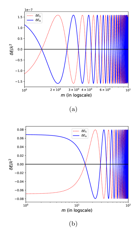
Figure 1: Dependence of energy shifts w.r.t mass of the scalar field for $\omega_{0}^{2}>m^{2}$. (a) for $L>>l$ we take $L=1000$, $l=1$, $\omega_{0}=10$ and $m$ is varying from 1 to 10 (b) for $l>>L$ we take $L=1$, $l=1000$, $\omega_{0}=100$ and $m$ is varying from 1 to 100. Here $m,~{}L,~{}l,~{}\omega_{0}$ are in arbitrary units.

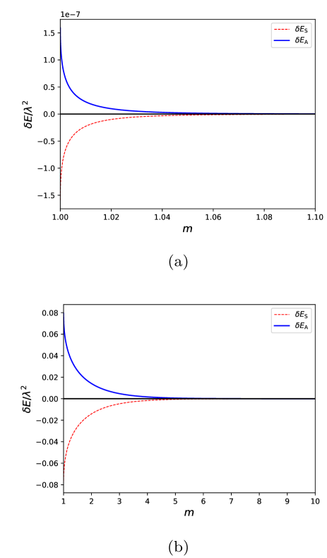
Figure 2: Dependence of energy shifts w.r.t mass of the scalar field for $\omega_{0}^{2}<m^{2}$. (a) for $L>>l$ we take $L=1000$, $l=1$, $\omega_{0}=1$ and $m$ is varying from 1 to 1.1 (b) for $l>>L$ we take $L=1$, $l=1000$, $\omega_{0}=1$ and $m$ is varying from 1 to 10. Here $m,~{}L,~{}l,~{}\omega_{0}$ are in arbitrary units.

IV.1 Case-I, $\omega_{0}^{2}>m^{2}$

For case-I, the poles of the integrand (33) lie on the real-line. Therefore, the expressions for Lamb shift of two atoms are given by,

$$\delta E_{S} = -\frac{\lambda^{2}}{4\pi L\sqrt{1+\frac{L^{2}}{4l^{2}}}}\cos(2\sqrt{\omega_{0}^{2}-m^{2}}\,\,l\sinh^{-1}\big{(}L/2l\big{)})~{},$$

$$\delta E_{A} = \frac{\lambda^{2}}{4\pi L\sqrt{1+\frac{L^{2}}{4l^{2}}}}\cos(2\sqrt{\omega_{0}^{2}-m^{2}}\,\,l\sinh^{-1}\big{(}L/2l\big{)}).$$

We also note that there exists a characteristic length scale $l$, which up to the leading order approximation is equal to $\frac{\sqrt{1-\frac{r_{s}}{r}}}{\kappa}$, where $\kappa=\frac{1}{2r_{s}}$ is the surface gravity [29]. To analyze the behavior of the RCPI, here we also consider both the limits of the proper distance between the atoms which are either larger or smaller than the characteristic length scale. From equation (IV.1), it is shown that in the limit $L>>l$ (or $\Delta\theta>>2\sqrt{\frac{\delta}{r_{s}}}$) [29], the expressions are,

$$\delta E_{S} = -\frac{\lambda^{2}~{}l}{2\pi L^{2}}\cos(2\sqrt{\omega_{0}^{2}-m^{2}}\,\,l\log(L/l))~{},$$

$$\delta E_{A} = \frac{\lambda^{2}~{}l}{2\pi L^{2}}\cos(2\sqrt{\omega_{0}^{2}-m^{2}}\,\,l\log(L/l))~{},$$ (35)

and in the limit $L<<l$ (or $\Delta\theta<<2\sqrt{\frac{\delta}{r_{s}}}$),

$$\delta E_{S} = -\frac{\lambda^{2}}{4\pi L}\cos(\sqrt{\omega_{0}^{2}-m^{2}}\,\,L)~{},$$

$$\delta E_{A} = \frac{\lambda^{2}}{4\pi L}\cos(\sqrt{\omega_{0}^{2}-m^{2}}\,\,L)~{}.$$ (36)

The schematic diagrams for both the limits are shown in FIG. 1.

IV.2 Case-II, $\omega_{0}^{2}<m^{2}$

For case-II, the poles in the integrand (33) lie on the imaginary axis, the expressions for RCPI are given by,

$$\delta E_{S} = -\frac{\lambda^{2}}{4\pi L\sqrt{1+\frac{L^{2}}{4l^{2}}}}e^{-2\sqrt{m^{2}-\omega_{0}^{2}}\,\,l\sinh^{-1}\big{(}L/2l\big{)}}~{},$$

$$\delta E_{A} = \frac{\lambda^{2}}{4\pi L\sqrt{1+\frac{L^{2}}{4l^{2}}}}e^{-2\sqrt{m^{2}-\omega_{0}^{2}}\,\,l\sinh^{-1}\big{(}L/2l\big{)}}~{}.$$ (37)

The expressions have an exponential decaying term, which indicates the same kind of result of the two-point correlation function at $mR>>1$. Therefore, the correlation function and RCPI vanish in the large mass limit. From equation (IV.1), in the limit $L>>l$ (or $\Delta\theta>>2\sqrt{\frac{\delta}{r_{s}}}$), the expressions are given by,

$$\delta E_{S} = -\frac{\lambda^{2}~{}l}{2\pi L^{2}}e^{-2\sqrt{m^{2}-\omega_{0}^{2}}\,\,l\log(L/l)}~{},$$

$$\delta E_{A} = \frac{\lambda^{2}~{}l}{2\pi L^{2}}e^{-2\sqrt{m^{2}-\omega_{0}^{2}}\,\,l\log(L/l)}~{},$$ (38)

and in the limit $L<<l$ (or $\Delta\theta<<2\sqrt{\frac{\delta}{r_{s}}}$),

$$\delta E_{S} = -\frac{\lambda^{2}}{4\pi L}e^{-\sqrt{m^{2}-\omega_{0}^{2}}\,\,L}~{},$$

$$\delta E_{A} = \frac{\lambda^{2}}{4\pi L}e^{-\sqrt{m^{2}-\omega_{0}^{2}}\,\,L}~{}.$$ (39)

The schematic diagrams for both the limits are shown in FIG. 2 .

IV.3 Case-III, $\omega_{0}^{2}=m^{2}$

For case-III, the pole of the integrand (33) is at the origin, $z=0$. The expressions for RCPI are shown below,

$$\delta E_{S} = -\frac{\lambda^{2}}{4\pi L\sqrt{1+\frac{L^{2}}{4l^{2}}}},$$

$$\delta E_{A} = \frac{\lambda^{2}}{4\pi L\sqrt{1+\frac{L^{2}}{4l^{2}}}}.$$ (40)

From equation (IV.2), in the limit $L>>l$ (or $\Delta\theta>>2\sqrt{\frac{\delta}{r_{s}}}$), the expressions are given by,

$$\delta E_{S} = -\frac{\lambda^{2}~{}l}{2\pi L^{2}},$$

$$\delta E_{A} = \frac{\lambda^{2}~{}l}{2\pi L^{2}},$$ (41)

and in the limit $L<<l$ (or $\Delta\theta<<2\sqrt{\frac{\delta}{r_{s}}}$),

$$\delta E_{S} = -\frac{\lambda^{2}}{4\pi L},$$

$$\delta E_{A} = \frac{\lambda^{2}}{4\pi L}~{}.$$ (42)

Both the FIG. 1 and FIG. 2 merge at the same point for $\omega_{0}=m$. We also check analytically the pair of equations, (IV.1,IV.2) are equal with the expression (IV.3) and similarly for (IV.1,IV.2) are equal with (IV.3). However, The length scale limit beyond a characteristic value ($L>>l$) for the three cases (IV.1,IV.2,IV.3) is not compatible with the local flatness of the spacetime [29].

V Discussions

From the analogy of equivalence principle we can say an accelerating observer mimics an observer in a gravitational field and from thermalization theorem we find a connection between an accelerating atom and a quantum system connected to a thermal bath. Therefore, we use the quantum master equation approach to describe the dynamics of an accelerating two-atom system interacting with a massive scalar field. We find the expressions for the second-order shift term for system-field coupling Hamiltonian. In the presence of vacuum fluctuations of the field, the effective shift terms are responsible for the interatomic correlations between the atoms. Here we calculate the RCPI for the Schwarzschild spacetime in the near-horizon region. From the recent studies, the RCPI using a massless scalar field beyond a characteristic length scale follows a $1/L^{2}$ power-law behavior [29]. The length-scale is equivalent to the inverse of the surface gravity $\kappa$ in Schwarzschild spacetime. However, the limit is not compatible with the locally flat space-time. For the massive scalar field, we also find the same kind of behavior. With this characteristic length scale, we also introduce a mass dependence of RCPI, which serves another independent length scale in the dynamics. The key point we have addressed here is both the limits ($\omega_{0}^{2}>m^{2},\omega_{0}^{2}<m^{2}$) merge to a constant-value which is independent of the mass of scalar field and the frequency of Zeeman levels. There is a competition between the frequency of Zeeman levels and the mass of the scalar field when they are equal the energy-shifts become maximum. This particular value exactly shows the behavior of a two-atom system whose frequency of Zeeman levels is zero in a massless scalar field. In summary, we have shown that in the low mass limit it exactly follows the behavior reported in ref. [29] with the frequency modulated by a mass term and in the high mass limit, the behavior of RCPI becomes short-range and eventually disappears beyond a characteristic length scale of $1/m$. So, the atoms become uncorrelated in the large mass limit.

- [1] H. B. G. Casimir and D. Polder. The Influence of Retardation on the London-van der Waals Forces. Physical Review, 73(4):360–372, February 1948.
- [2] Michael Bordag. The Casimir Effect 50 Years Later. WORLD SCIENTIFIC, 1999.
- [3] Casimir Physics. Lecture Notes in Physics. Springer-Verlag, Berlin Heidelberg, 2011.
- [4] R. L. Jaffe. Casimir effect and the quantum vacuum. Physical Review D, 72(2):021301, July 2005.
- [5] P. R. Berman. Cavity quantum electrodynamics. 1994.
- [6] Zehua Tian, Jieci Wang, Jiliang Jing, and Andrzej Dragan. Detecting the Curvature of de Sitter Universe with Two Entangled Atoms. Scientific Reports, 6:35222, 2016.
- [7] Luis G. MacDowell. Surface van der Waals forces in a nutshell. The Journal of Chemical Physics, 150(8):081101, February 2019.
- [8] G. L. Klimchitskaya and V. M. Mostepanenko. Casimir and van der Waals forces: Advances and problems. Proceedings of Peter the Great St. Petersburg Polytechnic University, (517):41–65, June 2015. arXiv: 1507.02393.
- [9] Yu-ju Lin, Igor Teper, Cheng Chin, and Vladan Vuletić. Impact of the Casimir-Polder Potential and Johnson Noise on Bose-Einstein Condensate Stability Near Surfaces. Physical Review Letters, 92(5):050404, February 2004.
- [10] D. M. Harber, J. M. Obrecht, J. M. McGuirk, and E. A. Cornell. Measurement of the Casimir-Polder force through center-of-mass oscillations of a Bose-Einstein condensate. Physical Review A, 72(3):033610, September 2005.
- [11] Zehua Tian and Jiliang Jing. Distinguishing de Sitter universe from thermal Minkowski spacetime by Casimir-Polder-like force. JHEP, 07:089, 2014.
- [12] Jialin Zhang and Hongwei Yu. Far-zone interatomic casimir-polder potential between two ground-state atoms outside a schwarzschild black hole. Phys. Rev. A, 88:064501, Dec 2013.
- [13] L. Rizzuto. Casimir-polder interaction between an accelerated two-level system and an infinite plate. Phys. Rev. A, 76:062114, Dec 2007.
- [14] Jamir Marino, Antonio Noto, and Roberto Passante. Thermal and Nonthermal Signatures of the Unruh Effect in Casimir-Polder Forces. Phys. Rev. Lett., 113(2):020403, 2014.
- [15] Lucia Rizzuto, Margherita Lattuca, Jamir Marino, Antonio Noto, Salvatore Spagnolo, Roberto Passante, and Wenting Zhou. Nonthermal effects of acceleration in the resonance interaction between two uniformly accelerated atoms. Phys. Rev., A94(1):012121, 2016.
- [16] Gabriel Menezes, Claus Kiefer, and Jamir Marino. Thermal and nonthermal scaling of the Casimir-Polder interaction in a black hole spacetime. Phys. Rev., D95(8):085014, 2017.
- [17] Hong Wei Yu and Jialin Zhang. Understanding Hawking radiation in the framework of open quantum systems. Phys. Rev., D77:024031, 2008.
- [18] Wenting Zhou and Hongwei Yu. Resonance interatomic energy in a Schwarzschild spacetime. Phys. Rev., D96(4):045018, 2017.
- [19] Xiaobao Liu, Zehua Tian, Jieci Wang, and Jiliang Jing. Radiative process of two entanglement atoms in de sitter spacetime. Phys. Rev. D, 97:105030, May 2018.
- [20] Greg Ver Steeg and Nicolas C. Menicucci. Entangling power of an expanding universe. Phys. Rev. D, 79:044027, Feb 2009.
- [21] Jiawei Hu and Hongwei Yu. Quantum entanglement generation in de sitter spacetime. Phys. Rev. D, 88:104003, Nov 2013.
- [22] Grant Salton, Robert B Mann, and Nicolas C Menicucci. Acceleration-assisted entanglement harvesting and rangefinding. New Journal of Physics, 17(3):035001, mar 2015.
- [23] S. Felicetti, M. Sanz, L. Lamata, G. Romero, G. Johansson, P. Delsing, and E. Solano. Dynamical Casimir Effect Entangles Artificial Atoms. Physical Review Letters, 113(9):093602, August 2014.
- [24] Xavier Busch, Renaud Parentani, and Scott Robertson. Quantum entanglement due to modulated Dynamical Casimir Effect. Phys. Rev. A, 89(6):063606, June 2014. arXiv: 1404.5754.
- [25] M. A Cirone, G Compagno, G. M Palma, R Passante, and F Persico. Casimir-polder potentials as entanglement probe. Europhysics Letters, 78(3):30003, apr 2007.
- [26] Phys. Rev. Lett. 89, 277901 (2002) - Creation of Entanglement by Interaction with a Common Heat Bath.
- [27] Fabio Benatti, Roberto Floreanini, and Marco Piani. Environment Induced Entanglement in Markovian Dissipative Dynamics. Physical Review Letters, 91(7):070402, August 2003.
- [28] F. Benatti and R. Floreanini. Entanglement generation in uniformly accelerating atoms: Reexamination of the unruh effect. Phys. Rev. A, 70:012112, Jul 2004.
- [29] Chiranjeeb Singha. Remarks on distinguishability of Schwarzschild spacetime and thermal Minkowski spacetime using Resonance Casimir–Polder interaction. Modern Physics Letters A, page 1950356, October 2019.
- [30] Shin Takagi. Vacuum Noise and Stress Induced by Uniform Acceleration: Hawking-Unruh Effect in Rindler Manifold of Arbitrary Dimension. Progress of Theoretical Physics Supplement, 88:1–142, 03 1986.
- [31] The Theory of Open Quantum Systems - Heinz-Peter Breuer, Francesco Petruccione - Oxford University Press.
- [32] A. Laliotis and M. Ducloy. Casimir-Polder effect with thermally excited surfaces. Physical Review A, 91(5):052506, May 2015.
- [33] L. Hollberg and J. L. Hall. Measurement of the Shift of Rydberg Energy Levels Induced by Blackbody Radiation. Physical Review Letters, 53(3):230–233, July 1984.
- [34] G. Lindblad. On the generators of quantum dynamical semigroups. Communications in Mathematical Physics, 48(2):119–130, 1976.
- [35] On quantum statistical mechanics of non-Hamiltonian systems. 3(4).
- [36] E.B. Davis. Quantum Theory of Open Systems. Academic Press, 1976.
- [37] Gilbert Grynberg Claude Cohen-Tannoudji, Jacques Dupont-Roc. Atom-Photon Interactions: Basic Processes and Applications.
- [38] Daniel V. Schroeder and Michael E. Peskin. An Introduction to quantum field theory. 1995.
- [39] Entangled states and collective nonclassical effects in two-atom systems. Physics Reports, 372(5):369 – 443, 2002.
- [40] Badis Ydri. Quantum Black Holes. 2017.
- [41] Joseph Polchinski. The Black Hole Information Problem. In Proceedings, Theoretical Advanced Study Institute in Elementary Particle Physics: New Frontiers in Fields and Strings (TASI 2015): Boulder, CO, USA, June 1-26, 2015, pages 353–397, 2017.
- [42] Atish Dabholkar and Suresh Nampuri. Quantum black holes. Lect. Notes Phys., 851:165–232, 2012.
- [43] Kanato Goto and Yoichi Kazama. On the observer dependence of the Hilbert space near the horizon of black holes. PTEP, 2019(2):023B01, 2019.
- [44] N. D. Birrell and P. C. W. Davies. Quantum Fields in Curved Space by N. D. Birrell, February 1982.
- [45] Chandramouli Chowdhury, Ashmita Das, and Bibhas Ranjan Majhi. Unruh-DeWitt detector in the presence of multiple scalar fields: A toy model. The European Physical Journal Plus, 134(2):65, February 2019.