Analyticity and $hp$ discontinuous Galerkin approximation of nonlinear Schrödinger eigenproblems

Abstract.

We study a class of nonlinear eigenvalue problems of Schrödinger type, where the potential is singular on a set of points. Such problems are widely present in physics and chemistry, and their analysis is of both theoretical and practical interest. In particular, we study the regularity of the eigenfunctions of the operators considered, and we propose and analyze the approximation of the solution via an isotropically refined $hp$ discontinuous Galerkin (dG) method.

We show that, for weighted analytic potentials and for up-to-quartic polynomial nonlinearities, the eigenfunctions belong to analytic-type non homogeneous weighted Sobolev spaces. We also prove quasi optimal a priori estimates on the error of the dG finite element method; when using an isotropically refined $hp$ space the numerical solution is shown to converge with exponential rate towards the exact eigenfunction. We conclude with a series of numerical tests to validate the theoretical results.

1. Introduction

This paper concerns the analysis of an elliptic nonlinear eigenvalue problem and its approximation with an $hp$ discontinuous Galerkin finite element method. Specifically, we consider the problem of finding, in a domain $\Omega\subset\mathbb{R}^{d}$, $d=2,3$, the smallest eigenvalue and associated eigenfunction $(\lambda,u)$ such that $\|u\|_{L^{2}(\Omega)}=1$ and

(1) $$(-\Delta+V+f(u^{2}))u=\lambda u,$$

for a (singular) potential $V$ and a nonlinearity $f$. We refer to Ref. [4] and the references therein for a discussion of problem (1) and its connections with models in physics. In this manuscript, we will perform a theoretical analysis of (1) with periodic boundary conditions, and we will investigate the behavior of the numerical scheme with homogeneous Dirichlet boundary conditions.

We prove weighed analytic regularity and exponential convergence of the $hp$ method for nonlinearities $f(u^{2})u=|u|^{n-1}u$ with $n=2,3,4$, i.e., an up-to-quartic polynomial nonlinearity. Problems of this kind correspond to the Euler-Lagrange equations of energy minimization problems and are therefore widely present in physics and chemistry. Equations of the form (1) are also often referred to as nonlinear Schrödinger equations. Problem (1) also constitutes a model for problems of wide interest in quantum chemistry, such as the Hartree-Fock model. The latter is, indeed, a nonlinear elliptic eigenvalue problem, with a singular potential, and with a nonlinearity that is cubic in nature. The main difference with what we consider here is that our nonlinearity is local, and that we only consider the smallest eigenvalue.

Our analysis is centered mainly on potentials that are singular at a set of isolated points; this includes the electric attraction generated by a Coulomb potential, i.e., $V(x)=1/d(x,{\mathfrak{c}})$, where $d(\cdot,\cdot)$ is the euclidean distance between two points in $\mathbb{R}^{d}$, for some fixed point ${\mathfrak{c}}\in\Omega$, but applies more generally to any potential that, in the vicinity of the singular point, behaves as

(2) $$V(x)\sim\frac{1}{d(x,{\mathfrak{c}})^{\xi}},$$

for a $\xi<2$. Clearly, $V$ is not very regular in classical Sobolev spaces, thus we cannot expect the solution to be regular in those spaces either. Nonetheless, we can alternatively work in weighted Kondrat’ev-Babuška spaces, prove that the solution is sufficiently regular in these spaces, and thus design an appropriate $hp$ discretization that converges exponentially to the exact solution, see Ref. [23].

The nonlinear Schrödinger equation (1) and the weighted spaces are introduced in detail in Section 2. There, we also introduce our basic assumptions on the nonlinearity, which are similar to those introduced in Ref. [4], and on the potential $V$. As the analysis progresses, we will introduce more restrictive hypotheses.

In Section 3, we then prove a priori convergence estimates on the eigenvalue and eigenfunction. We consider a wider class of nonlinearities than polynomial ones, as detailed in equations (7a) to (7d). Even though our focus is on $hp$ methods, the abstract convergence proofs in Section 3 do not exploit specific features of $hp$ methods, and cover also other discretizations. Suppose we consider a simpler $h$-type finite element method: the proof of Theorem 1 — i.e., convergence and quasi optimality of the numerical solution — holds, since we do not use any specific feature of $hp$ refinement. The proof of convergence of the discontinuous Galerkin method for a nonlinear eigenvalue problem of the form (1) is a new result as far as we are aware. Previous results include the convergence of the discontinuous Galerkin method for linear eigenproblems [1] and the convergence of conforming methods for the nonlinear problem [4]. The main difference with the latter paper is that the discontinuous Galerkin method is not conforming, thus some relations between exact and numerical quantities, e.g., between the exact eigenvalue $\lambda$ and the numerical one ${\lambda_{\delta}}$, are less straightforward. In general, the convergence and quasi optimality of the numerical eigenvalue–eigenfunction pair proven in Theorem 1 should be readily extendable to any nonconforming symmetric method such that the thesis of Lemma 3, akin to coercivity and continuity of the numerical bilinear form, holds.

In Section 4, we restrict the analysis to the case of polynomial, up-to-quartic polynomial nonlinearities. In this setting, the solutions of problem (1) are analytic in weighted Sobolev spaces: specifically, if the potential is of type (2) and $f(u^{2})=|u|^{n-1}$, $n=2,3,4$, then for $\gamma<d/2+2-\xi$ there exist constants $C_{u}$ and $A_{u}$ such that for all $k\in\mathbb{N}$

$$\sum_{{|\alpha|}=k}\|d(x,{\mathfrak{c}})^{k-\gamma}\partial^{\alpha}u\|_{L^{2}(\Omega)}\leq C_{u}A_{u}^{k}k!,$$

where $u$ is the ground state of (1) and $\alpha\in\mathbb{N}_{0}^{d}$ is a multi index. This weighted, analytic regularity estimate is proven in Theorem 2 and constitutes a novel result of independent interest. For previous weighted analytic regularity results for elliptic problems, we refer, among others, to Refs. [12, 7].

As a consequence of the quasi-optimal a priori estimates introduced above and of the weighted analytic regularity of the ground state for up-to-quartic nonlinearities, we obtain exponential convergence of the numerical solution computed with the $hp$ dG method. This is briefly discussed in Section 5 and presented in Theorem 3.

Finally, in Section 6, we investigate the performance of the scheme in two and three dimensional numerical tests. We confirm our theoretical estimates, while also showing the effect of sources of numerical error that have not been taken into consideration in the theoretical analysis.

2. Statement of the problem and notation

2.1. Functional setting and notation

Let $\Omega=\mathbb{R}^{d}/(L\mathbb{Z})^{d}$ be the flat torus of period $0<L\leq 1$ and let $S=(0,L)^{d}$. We use the standard notation for Sobolev spaces, that we indicate, for any non periodic set $D\subset\mathbb{R}^{d}$, as $W^{k,p}(D)$, with $W^{k,2}(D)=H^{k}(D)$ and $W^{0,p}(D)=L^{p}(D)$. We write $v\in W_{\mathrm{loc}}^{k,p}(\mathbb{R}^{d})$ if, for all bounded $D\subset\mathbb{R}^{d}$, $v\in W^{k,p}(D)$. Furthermore, we indicate periodized Sobolev spaces on $\Omega$ by

$$W^{k,p}(\Omega)=W_{\mathrm{per}}^{k,p}(S)=\left\{v_{|_{S}}:v\in W_{\mathrm{loc}}^{k,p}(\mathbb{R}^{d})\text{ and }v_{|_{S+iL}}=v_{|_{S}}\text{ for all }i\in\mathbb{Z}^{d}\right\},$$

with $H^{k}(\Omega)=H_{\mathrm{per}}^{k}(S)=W^{k,2}(\Omega)$ and $L^{p}(\Omega)=L_{\mathrm{per}}^{p}(S)=W^{0,p}(\Omega)$. We denote the scalar product in $L^{2}(D)$, for $D\subset\mathbb{R}^{d}$, as $(\cdot,\cdot)_{D}$, the scalar product in $L_{\mathrm{per}}^{2}(\Omega)$ as $(\cdot,\cdot)$, and the respective norm as $\lVert u\rVert=(u,u)^{1/2}$. Furthermore, we denote by $\mathbb{N}$ the set of strictly positive natural numbers, and by $\mathbb{N}_{0}=\mathbb{N}\cup\{0\}$. For two quantities $a$ and $b$, we write $a\lesssim b$ (respectively $a\gtrsim b$) if there exists $C>0$ independent of the discretization, such that $a\leq Cb$ (resp. $a\geq Cb$). We write $a\simeq b$ if $a\lesssim b$ and $a\gtrsim b$.

We now recall the definition of the weighted Sobolev spaces, introduced in Ref. [14], that will be central to our regularity analysis. Given a set of isolated points ${\mathfrak{C}}\subset S$, we write $\widetilde{\mathfrak{C}}=\{\mathfrak{C}+kL,\,k\in\mathbb{Z}^{d}\}$. we introduce the homogeneous Kondrat’ev-Babuška space $\mathcal{K}^{k,p}_{\gamma}(\Omega,\mathfrak{C})$, defined as

$$\mathcal{K}^{k,p}_{\gamma}(\Omega,\mathfrak{C})=\{u_{|_{S}}:u\in W_{\mathrm{loc}}^{k,p}(\mathbb{R}^{d}\setminus\widetilde{\mathfrak{C}}),\,u_{|_{S}}=u_{|S+iL}\,\forall i\in\mathbb{Z}^{d},\\ \text{ and }r^{|\alpha|-\gamma}(\partial^{\alpha}u)_{|_{S}}\in L^{p}(S)\;\forall\alpha\in\mathbb{N}_{0}^{d}:|\alpha|\leq k\},$$

where $r=r(x)$ is any smooth function defined on $S$ which is, in the vicinity of every point ${\mathfrak{c}}\in\mathfrak{C}$, equal to the euclidean distance $d(x,{\mathfrak{c}})$ from the point and nonzero elsewhere. For example,

$$r(x)=\prod_{{\mathfrak{c}}\in{\mathfrak{C}}}d(x,{\mathfrak{c}}),\qquad\forall x\in S.$$

The nonhomogeneous Kondrat’ev-Babuška space is defined by

$$\mathcal{J}^{k,p}_{\gamma}(\Omega,\mathfrak{C})=\{u_{|_{S}}:u\in W_{\mathrm{loc}}^{\lfloor\gamma-d/p\rfloor,p}(\mathbb{R}^{d})\cap W_{\mathrm{loc}}^{k,p}(\mathbb{R}^{d}\setminus\widetilde{{\mathfrak{C}}}),\,u_{|_{S}}=u_{|_{S+iL}}\,\forall i\in\mathbb{Z}^{d}\\ \text{and }r^{{|\alpha|}-\gamma}(\partial^{\alpha}u)_{|_{S}}\in L^{p}(S)\;\forall\alpha\in\mathbb{N}^{d}:\lfloor\gamma-d/p\rfloor+1\leq|\alpha|\leq k\},$$

for $\gamma>d/p$. We define the associated seminorm as

$$|u|_{\mathcal{J}^{k,p}_{\gamma}(\Omega)}=|u|_{\mathcal{K}^{k,p}_{\gamma}(\Omega)}=\sum_{{|\alpha|}=k}\|r^{{|\alpha|}-\gamma}\partial^{\alpha}u\|_{L^{p}(S)}.$$

We also introduce the spaces of regular functions with weighted analytic type estimates as

$$\mathcal{K}^{\varpi,p}_{\gamma}(\Omega,\mathfrak{C})=\{v\in\mathcal{K}^{\infty,p}_{\gamma}(\Omega,\mathfrak{C}):|v|_{\mathcal{K}^{k,p}_{\gamma}(\Omega)}\leq CA^{k}k!\;\forall k\in\mathbb{N}_{0}\},$$

and

$$\mathcal{J}^{\varpi,p}_{\gamma}(\Omega,\mathfrak{C})=\{v\in\mathcal{J}^{\infty,p}_{\gamma}(\Omega,\mathfrak{C}):|v|_{\mathcal{K}^{k,p}_{\gamma}(\Omega)}\leq CA^{k}k!,\;\forall k\in\mathbb{N}_{0}:k\geq\lfloor\gamma-d/p\rfloor+1\},$$

where $\mathcal{K}^{\infty,p}_{\gamma}(\Omega)=\bigcap_{k}\mathcal{K}^{k,p}_{\gamma}(\Omega)$, $\mathcal{J}^{\infty,p}_{\gamma}(\Omega)$ defined similarly. To simplify the notation, we will suppose that there is only one singular point per cell $S$, i.e., ${\mathfrak{C}}=\{{\mathfrak{c}}\}$ and omit $\mathfrak{C}$ from the notation of the spaces. Furthermore, we write $\mathcal{K}^{k}_{\gamma}(\Omega)=\mathcal{K}^{k,2}_{\gamma}(\Omega)$, $\mathcal{J}^{k}_{\gamma}(\Omega)=\mathcal{J}^{k,2}_{\gamma}(\Omega)$, $\mathcal{K}^{\varpi}_{\gamma}(\Omega)=\mathcal{K}^{\varpi,2}_{\gamma}(\Omega)$, and $\mathcal{J}^{\varpi}_{\gamma}(\Omega)=\mathcal{J}^{\varpi,2}_{\gamma}(\Omega)$. For a thorough treatment of Kondrat’ev-Babuška spaces, see Refs. [15, 5, 6, 7]. Note that the results obtained in the sequel can be trivially extended to the case where ${\mathfrak{C}}$ contains more than one point, as long as ${\mathfrak{C}}$ is a finite set of points. When, for any non periodic set $D\subset\mathbb{R}^{d}$, we refer to the spaces $\mathcal{J}^{k,p}_{\gamma}(D)$, we implicitly refer to their non periodized version.

Finally, let $X=\mathcal{J}^{2}_{\gamma}(\Omega)$, for $\gamma\in(d/2,d/2+\varepsilon)$, where $0<\varepsilon<1$ will be specified later, namely in hypothesis (8b).

Remark 1.

We perform our analysis in the torus $\Omega=\mathbb{R}^{d}/(L\mathbb{Z})^{d}$ to avoid having to deal with the singularities that arise at the edges of polyhedral domains. A theory of weighted analytic regularity for nonlinear elliptic problems in polyhedral domains is, indeed, not available in the literature; the analysis we perform here can be also applied to corner singularities of solutions to nonlinear elliptic problems in polyhedral domain, and can be therefore seen as a first building block for the analysis of nonlinear elliptic problems in polyhedral domains.

2.2. Statement of the problem

We introduce the problem under consideration. From the “physical” point of view, it consists in the minimization of an energy composed by a kinetic term, an interaction with a singular potential $V$ and a nonlinear self-interaction term. Under the unitary norm constraint, using Euler’s equation, the energy minimization problem translates into a nonlinear elliptic eigenvalue problem. This is the form under which most of the analysis will be carried out.

We start therefore by introducing the bilinear form over $H^{1}(\Omega)\times H^{1}(\Omega)$

(3) $$a(u,v)=\int_{\Omega}\nabla u\cdot\nabla v+\int_{\Omega}Vuv$$

and a function $F:\mathbb{R}^{+}\to\mathbb{R}$, whose properties have been introduced in Section 1. Let

(4) $$E(v)=\frac{1}{2}a(v,v)+\frac{1}{2}\int_{\Omega}F(v^{2}).$$

Let us denote by $u$ the minimizer of (4) (unique up to a sign change under the hypotheses that follow) over the space $\{v\in H^{1}(\Omega):\lVert v\rVert=1\}$: then, there exists $\lambda\in\mathbb{R}$ such that $u$ is the solution of

(5) $$\langle A^{u}u-\lambda u,v\rangle=0\quad\forall v\in H^{1}(\Omega)$$

where for given $u\in H^{1}(\Omega)$, $A^{u}\in\mathcal{L}(H^{1}(\Omega),(H^{1}(\Omega))^{\prime})$ is defined as

$$\langle A^{u}v,w\rangle=a(v,w)+\int_{\Omega}f(u^{2})vw,$$

with $f=F^{\prime}$. We introduce also

(6) $$\langle E^{\prime\prime}(u)v,w\rangle=\langle A^{u}v,w\rangle+2\int_{\Omega}f^{\prime}(u^{2})u^{2}vw,\qquad\forall v,w\in H^{1}(\Omega).$$

The properties of the function $F$ will be similar to those in Ref. [4] and have already been introduced above. We recall them here:

(7a) $$F\in C^{1}([0,+\infty),\mathbb{R})\cap C^{\infty}((0,+\infty),\mathbb{R})\text{ and }F^{\prime\prime}>0\text{ in }(0,+\infty),$$

(7b) $$\exists q\in[0,2),\exists C\in\mathbb{R}:\forall t\geq 0,|F^{\prime}(t)|\leq C(1+t^{q}),$$

(7c) $$F^{\prime\prime}(t)t\text{ locally bounded in }[0,+\infty),$$

and we suppose that $$\forall R>0,\exists C_{R}\in\mathbb{R}_{+}:\forall t_{1}\in(0,R],\forall t_{2}\in\mathbb{R}$$,

(7d) $$\lvert F^{\prime}(t_{2}^{2})t_{2}-F^{\prime}(t_{1}^{2})t_{2}-2F^{\prime\prime}(t_{1}^{2})(t_{1}^{2})(t_{2}-t_{1})\rvert\leq C_{R}(1+|t_{2}|^{s})|t_{2}-t_{1}|^{r}$$

for $r\in(1,2]$ and $s\in[0,5-r)$. As an example of nonlinearities satisfying (7a) to (7d), we mention, following Ref. [4], functions modeling repulsive interaction in Bose–Einstein condensates ($F(t)\propto t^{2}$) and the Thomas–Fermi kinetic energy functional ($F(t)\propto t^{5/3}$). We refer the reader to the discussion in the mentioned reference.

Finally, we suppose that the potential $V$ is such that

(8a) $$V\in L^{p_{V}}(\Omega)$$

with $$p_{V}>\max(1,d/2) 0<\varepsilon<1$$ and that there exists such that

(8b) $$V\in\mathcal{K}^{\varpi,{}\infty}_{-2+\varepsilon}(\Omega,\mathfrak{C}).$$

For $d=2,3$, (8b) implies (8a) as long as $p_{V}<d/(2-\varepsilon)$. A consequence of (8a) is, in particular, that for $u,v\in H^{1}(\Omega)$,

$$(Vu,v)\leq C\|u\|_{H^{1}(\Omega)}\|v\|_{H^{1}(\Omega)}.$$

where the constant $C$ depends on $V$ and on the domain.

Remark 2.

As an example of a class of potentials satisfying (8b), we mention the functions $V:\mathbb{R}^{d}\to\mathbb{R}$ such that

$$V(x)=\sum_{k\in\mathbb{Z}^{d}}\frac{1}{\exp(d(x,k)^{\beta})-1},$$

for $\beta\in(0,2)$.

We have also the following regularity result, which follows from (7b) and (8b) and the regularity result obtained in Ref. [19].

Lemma 1.

The solution $u$ to (5), under hypotheses (7a) to (8b), belongs to the space

(9) $$u\in\mathcal{J}^{2}_{d/2+\alpha}(\Omega)$$

for any $\alpha<\varepsilon$, with $\varepsilon$ as in (8b).

Proof.

We have $u\in L^{\infty}(\Omega)$, see Ref. [4]. Hence, $u$ is the solution of $\left(-\Delta+V\right)u=\lambda u+f(u^{2})u$, with right hand side belonging to the space $\mathcal{J}^{0}_{d/2+\varepsilon-2}(\Omega)$. Since the operator $-\Delta+V$ is an isomorphism from $\mathcal{J}^{2}_{d/2+\alpha}(\Omega)$ to $\mathcal{J}^{0}_{d/2+\alpha-2}(\Omega)$ for $0<\alpha<\varepsilon$, see Ref. [19], we obtain the thesis. ∎

2.3. Numerical method

In this section we introduce the $hp$ discontinuous Galerkin method. Concerning the design of the $hp$ space, the setting is the one from Refs. [10, 11]. Let $\mathcal{T}$ be a triangulation of axiparallel quadrilateral ($d=2$) or hexahedral ($d=3$) elements of $\Omega$, such that $\bigcup_{K\in\mathcal{T}}\overline{K}=\overline{S}$, whose properties will be specified later. A $d-1$ dimensional face (edge, when $d=2$) is defined as the nonempty interior of $\partial K_{\sharp}\cap\partial K_{\flat}$ for two adjacent elements $K_{\flat}$ and $K_{\sharp}$. Let $\mathcal{E}$ be the set of all faces/edges. We denote

$$(u,v)_{\mathcal{T}}=\sum_{K\in\mathcal{T}}(u,v)_{K}$$

and, similarly,

$$(u,v)_{\mathcal{E}}=\sum_{e\in\mathcal{E}}(u,v)_{e}.$$

We suppose that for any $K\in\mathcal{T}$ there exists an affine transformation $\Phi:K\to{\hat{K}}$ to the $d$-dimensional cube ${\hat{K}}$ such that $\Phi(K)={\hat{K}}$, that the mesh is shape and contact regular.

We now introduce meshes that are isotropically and geometrically graded around the points in $\mathfrak{C}$: for simplicity, we consider the case where ${\mathfrak{C}}=\{{\mathfrak{c}}\}$. Then, we fix a refinement ratio $\sigma\in(0,1/2)$ and, for all $\ell\in\mathbb{N}$, we introduce a mesh $\mathcal{T}^{\ell}$ that can be partitioned into disjoint mesh layers $\mathcal{T}^{\ell}_{j}$, $j=1,\dots,\ell$ such that $\mathcal{T}^{\ell}={\bigcup}_{j=1}^{\ell}\mathcal{T}^{\ell}_{j}$. For all $K\in\mathcal{T}^{\ell}_{j}$, we suppose that

$$h_{K}\simeq h_{j}=\sigma^{j}\qquad d({\mathfrak{c}},K)\simeq h_{K},$$

for all $j=1,\dots,\ell$ and with constants uniform in $\mathcal{T}$ and $\ell$. Finally, we suppose that mesh refinement happens only at the singularity, i.e., given $\mathcal{T}^{\ell}=\mathcal{T}^{\ell}_{1}\cup\ldots\cup\mathcal{T}^{\ell}_{\ell}$, then $\mathcal{T}^{\ell+1}=\mathcal{T}^{\ell}_{1}{\cup}\ldots{\cup}\mathcal{T}^{\ell}_{\ell-1}{\cup}\mathcal{T}^{\ell+1}_{\ell}{\cup}\mathcal{T}^{\ell+1}_{\ell+1}$. The generalization to the case of ${\mathfrak{C}}$ containing multiple points follows from the construction of a graded mesh around each point.

We will allow for $1$-irregular edges/faces, i.e., given two neighboring elements $K_{\flat}$ and $K_{\sharp}$, that share an edge/face $e=\partial{K}_{\sharp}\cap\partial{K}_{\flat}$, we require that $e$ is an entire edge/face of at least one between $K_{\sharp}$ and $K_{\flat}$. We refer to Section 6 (specifically, to Figure 1(a)) for a visualization of such a mesh. We introduce on this mesh the $hp$ space with linear polynomial slope $s$, i.e., for an element $K\in\mathcal{T}^{\ell}$ such that $K\in\mathcal{T}^{\ell}_{j}$,

$$p_{K}\simeq p_{j}=p_{0}+\mathfrak{s}(\ell-j),$$

where $h_{K}$ is the diameter of the element $K$ and $p_{K}$ is the polynomial order whose role will be specified in (10). We introduce the discretization parameter $0<\delta\leq 1$ such that $\delta\to 0$ when $\ell\to\infty$, and the discrete space

(10) $$X_{\delta}=\left\{v_{\delta}\in L^{2}(\Omega):(v_{|_{K}}\circ\Phi^{-1})\in\mathbb{Q}_{p_{K}}({\hat{K}}),\,\forall K\in\mathcal{T}^{\ell}\right\},$$

where $\mathbb{Q}_{p}$ is the space of polynomials of maximal degree $p$ in any variable and denote

$$X(\delta)=X+{X_{\delta}}.$$

Then, $\mathcal{E}^{\ell}$ is the set of the edges (for $d=2$) or faces ($d=3$) of the elements in $\mathcal{T}^{\ell}$ and

$$\mathtt{h_{e}}=\min_{K\in\mathcal{T}^{\ell}:e\cap\partial K\neq\varnothing}h_{K},\qquad\mathtt{p_{e}}=\max_{K\in\mathcal{T}^{\ell}:e\cap\partial K\neq\varnothing}p_{K}.$$

On an edge/face between two elements $K_{\sharp}$ and $K_{\flat}$, i.e., on $e\subset\partial{K}_{\sharp}\cap\partial{K}_{\flat}$, the average $\{\!\!\{\cdot\}\!\!\}$ and jump $\llbracket\cdot\rrbracket$ operators for a function $w\in X(\delta)$ are defined by

$$\{\!\!\{w\}\!\!\}=\frac{1}{2}\left(w_{|_{K_{\sharp}}}+w_{|_{K_{\flat}}}\right),\qquad\llbracket w\rrbracket=w_{|_{K_{\sharp}}}\mathbf{n}_{\sharp}+w_{|_{K_{\flat}}}\mathbf{n}_{\flat},$$

where $\mathbf{n}_{\sharp}$ (resp. $\mathbf{n}_{\flat}$) is the outward normal to the element $K_{\sharp}$ (resp. $K_{\flat}$). If $e$ is an edge/face of an element $K$ and it lies on part of the boundary where homogeneous Dirichlet boundary conditions are imposed (as it will be the case in Section 6), the expression above is replaced by

$$\{\!\!\{w\}\!\!\}=w_{|_{K}},\qquad\llbracket w\rrbracket=w_{|_{K}}\mathbf{n},$$

where $\mathbf{n}$ is the normal pointing outwards from $K$.

We now introduce the discrete versions of the operators defined in Section 2.2. First, the bilinear form $a_{\delta}$ over $X_{\delta}\times X_{\delta}$ is given by

(11) $$a_{\delta}(u_{\delta},v_{\delta})=(\nabla u_{\delta},\nabla v_{\delta})_{\mathcal{T}^{\ell}} -(\{\!\!\{\nabla u_{\delta}\}\!\!\},\llbracket v_{\delta}\rrbracket)_{\mathcal{E}^{\ell}}-(\{\!\!\{\nabla v_{\delta}\}\!\!\},\llbracket u_{\delta}\rrbracket)_{\mathcal{E}^{\ell}}$$

$$+\sum_{e\in\mathcal{E}^{\ell}}\alpha_{e}\frac{\mathtt{p_{e}}^{2}}{\mathtt{h_{e}}}(\llbracket u_{\delta}\rrbracket,\llbracket v_{\delta}\rrbracket)_{e}+\int_{\Omega}Vu_{\delta}v_{\delta}.$$

Furthermore,

(12) $$E_{\delta}(v_{\delta})=\frac{1}{2}a_{\delta}(v_{\delta},v_{\delta})+\frac{1}{2}\int_{\Omega}F(v_{\delta}^{2}).$$

Let $u_{\delta}$ be a minimizer of (12) over ${X_{\delta}}$, with unitary norm constraint. Then, there exists an eigenvalue $\lambda_{\delta}\in\mathbb{R}$ such that

(13) $$\langle A_{\delta}^{u_{\delta}}u_{\delta}-\lambda_{\delta}u_{\delta},v_{\delta}\rangle=0\quad\forall v_{\delta}\in X_{\delta}$$

where

$$\langle A_{\delta}^{u_{\delta}}v_{\delta},w_{\delta}\rangle=a_{\delta}(v_{\delta},w_{\delta})+\int_{\Omega}f(u_{\delta}^{2})v_{\delta}w_{\delta}.$$

Finally, $E_{\delta}^{\prime\prime}$, defined on ${X_{\delta}}$, is obtained by replacing $A^{u}$ with $A_{\delta}^{u}$ in (6).

Remark 3 (Symmetry of the numerical method).

The dG method with bilinear form (11) is the symmetric interior penalty (SIP) method. The requirement of symmetry in the bilinear form of the numerical method is a strong one, and will be used without explicit mention throughout the proofs.

This could be seen as a limitation; nonetheless, from a practical point of view, there is little interest in approximating a symmetric eigenvalue problem with a non symmetric numerical method. Non symmetric methods tend to exhibit, in the linear case, lower rates of convergence than symmetric ones [1]. Furthermore, the solution of the finite dimensional problem would be more problematic, since algebraic eigenvalue problems are more easily treated for symmetric matrices [21].

We introduce the mesh dependent norms that will be used in this section. First, for a $v\in X(\delta)$,

(14) $$\lVert v\rVert_{\mathrm{DG}}^{2}=\sum_{K\in\mathcal{T}^{\ell}}\|v\|_{\mathcal{J}^{1}_{1}(K)}^{2}+\sum_{e\in\mathcal{E}^{\ell}}\mathtt{h_{e}}^{-1}{\mathtt{p_{e}}^{2}}\|\llbracket v\rrbracket\|_{L^{2}(e)}^{2}.$$

Remark that on $X$, this norm is equivalent to the $\mathcal{J}^{1}_{1}(\Omega)=H^{1}(\Omega)$ norm, since functions in $X$ have no face discontinuity, implying $\llbracket v\rrbracket=0$. Then, on $X(\delta)$ we introduce, when $d=3$,

(15) $$\left|\kern-1.07639pt\left|\kern-1.07639pt\left|u\right|\kern-1.07639pt\right|\kern-1.07639pt\right|_{\mathrm{DG}}^{2}=\sum_{K\in\mathcal{T}^{\ell}}\|u\|_{H^{1}(K)}^{2}+\sum_{e\in\mathcal{E}^{\ell}}\mathtt{p_{e}}^{2}\mathtt{h_{e}}^{-1}\|\llbracket u\rrbracket\|_{L^{2}(e)}^{2}+\sum_{e\in\mathcal{E}^{\ell}}\mathtt{p_{e}}^{-2}\|r^{1/2}\nabla u\cdot n_{e}\|_{L^{2}(e)}^{2},$$

where $n_{e}$ denotes the normal to face $e$. If $d=2$, we denote by $\mathcal{E}^{\ell}_{c}$ the set of edges abutting at the singularity, and write (note that on $\mathcal{E}^{\ell}_{c}$, $\mathtt{p_{e}}=p_{0}$)

(16) $$\left|\kern-1.07639pt\left|\kern-1.07639pt\left|u\right|\kern-1.07639pt\right|\kern-1.07639pt\right|_{\mathrm{DG}}^{2}=\sum_{K\in\mathcal{T}^{\ell}}\|u\|_{H^{1}(K)}^{2}+\sum_{e\in\mathcal{E}^{\ell}}\mathtt{p_{e}}^{2}\mathtt{h_{e}}^{-1}\|\llbracket u\rrbracket\|_{L^{2}(e)}^{2}+\sum_{e\in\mathcal{E}^{\ell}\setminus\mathcal{E}^{\ell}_{c}}\mathtt{p_{e}}^{-2}\|r^{1/2}{\nabla u}\cdot n_{e}\|_{L^{2}(e)}^{2}\\ +\sum_{e\in\mathcal{E}^{\ell}_{c}}\mathtt{h_{e}}^{q-1}\|\nabla u\cdot n_{e}\|_{L^{q}(e)}^{q},$$

where $q$ is fixed and such that $1<q<2/(3-\gamma)$, see Remark 4.

For any triangulation $\mathcal{T}$ of $\Omega$, let us also introduce the broken space

$$\mathcal{J}^{s,p}_{\gamma}(\Omega,\mathcal{T})=\left\{v:v\in\mathcal{J}^{{s,p}}_{\gamma}(K),\forall K\in\mathcal{T}\right\}.$$

Remark 4.

When $d=3$, by the definition of the weighted spaces, see Ref. [20], for $e\subset\partial K$, and since $\gamma>3/2$,

$$\|r^{1/2}\nabla v\|_{L^{2}(e)}\leq C\|v\|_{\mathcal{J}^{2}_{\gamma}(K)},$$

then $\left|\kern-1.07639pt\left|\kern-1.07639pt\left|v\right|\kern-1.07639pt\right|\kern-1.07639pt\right|_{\mathrm{DG}}$ (15) is bounded on $\mathcal{J}^{2}_{\gamma}(\Omega,\mathcal{T}^{\ell})$. Since furthermore $X(\delta)\subset\mathcal{J}^{2}_{\gamma}(\Omega,\mathcal{T}^{\ell})$, $\left|\kern-1.07639pt\left|\kern-1.07639pt\left|v\right|\kern-1.07639pt\right|\kern-1.07639pt\right|_{\mathrm{DG}}$ as defined in (15) is bounded when $d=3$ for all $v\in X(\delta)$.

When $d=2$, we consider the definition of the norm (16). Let $\gamma>1$: then, for any $q<2/(3-\gamma)$ and writing $t=(1/q-1/2)^{-1}$, there exist $C_{1},C_{2}$ such that, for all $v\in\mathcal{J}^{2}_{\gamma}(\Omega)$,

$$\sum_{{|\alpha|}=2}\|\partial^{\alpha}v\|_{L^{q}(\Omega)}\leq C_{1}\|r^{\gamma-2}\|_{L^{t}(\Omega)}\sum_{{|\alpha|}=2}\|r^{2-\gamma}\partial^{\alpha}v\|_{L^{2}(\Omega)}\leq C_{2}\|v\|_{\mathcal{J}^{2}_{\gamma}(\Omega)}.$$

Hence, if $v\in\mathcal{J}^{2}_{\gamma}(\Omega)$ with $\gamma>1$, $v\in W^{2,q}(\Omega)$, and $\|\nabla v\cdot n\|_{L^{q}(e)}$ is well defined. Therefore, $\left|\kern-1.07639pt\left|\kern-1.07639pt\left|v\right|\kern-1.07639pt\right|\kern-1.07639pt\right|_{\mathrm{DG}}$ as defined in (16) is bounded when $d=2$ for all $v\in X(\delta)$.

Remark 5.

By proving continuity as in Lemma 3 (see the part of the proof referring to inequality (21a)) and thanks to Remark 4, it can be shown that the bilinear form $a_{\delta}$ defined in (11) over ${X_{\delta}}\times{X_{\delta}}$ can be extended over $X(\delta)\times X_{\delta}$.

Remark 6.

Note that on $X_{\delta}$ and for $d\leq 3$, the two norms (14) and (15) are uniformly (with respect to the refinement level) equivalent, since for any $K\in\mathcal{T}^{\ell}$, $r_{|_{K}}\lesssim h_{K}$ and thanks to the discrete trace inequality [9]

(17) $$h_{e}^{(1-d)/p+d/2}\|w_{\delta}\|_{L^{p}(e)}\leq C_{d,p}\|w_{\delta}\|_{L^{2}(K)},$$

valid for $e\in\partial K$ and for all $w_{\delta}\in X_{\delta}$. The constant $C_{d,p}$ depends on the dimension $d$, on $p$, and on the polynomial order $\mathtt{p_{e}}$, but is independent of $\mathtt{h_{e}}$. Furthermore, $C_{d,p}$ is bounded by $\mathtt{p_{e}}$ if $p=2$.

Remark 7.

The coercivity of the SIP discrete bilinear form associated to the Laplacian, i.e., the existence of $c>0$ such that, for all ${v_{\delta}}\in{X_{\delta}}$

$$(\nabla v_{\delta},\nabla v_{\delta})_{\mathcal{T}}-(\{\!\!\{\nabla v_{\delta}\}\!\!\},\llbracket v_{\delta}\rrbracket)_{\mathcal{E}}-(\{\!\!\{\nabla v_{\delta}\}\!\!\},\llbracket v_{\delta}\rrbracket)_{\mathcal{E}}+\sum_{e\in\mathcal{E}}\alpha_{e}\frac{\mathtt{p_{e}}^{2}}{\mathtt{h_{e}}}(\llbracket v_{\delta}\rrbracket,\llbracket v_{\delta}\rrbracket)_{e}\geq c\lVert{v_{\delta}}\rVert_{\mathrm{DG}}^{2},$$

is verified if for all $e\in\mathcal{E}$, $\alpha_{e}>\alpha^{*}>0$, for some $\alpha^{*}$ that depends on the mesh. This is shown in Theorem 4.4 of Ref. [22] for geometrically graded meshes; for quasi-uniform meshes, see Refs. [24, 30, 18] for explicit expressions of $\alpha^{*}$.

We conclude this section by introducing the discrete approximation to the solution of the linear problem, i.e. the function $u_{\delta}^{*}\in X_{\delta}$ such that

(18) $$\langle A_{\delta}^{u}u_{\delta}^{*}-\lambda_{\delta}^{*}u_{\delta}^{*},v_{\delta}\rangle=0\quad\forall v_{\delta}\in X_{\delta}$$

for an eigenvalue $\lambda_{\delta}^{*}$. Note that, since $u$ is an eigenfunction of $A^{u}$ and the associated eigenspace is of dimension $1$ [4], we have that

(19) $$\lVert u_{\delta}^{*}-u\rVert_{\mathrm{DG}} \lesssim\inf_{v_{\delta}\in X_{\delta}}\left|\kern-1.07639pt\left|\kern-1.07639pt\left|u-v_{\delta}\right|\kern-1.07639pt\right|\kern-1.07639pt\right|_{\mathrm{DG}},$$

$$|\lambda_{\delta}^{*}-\lambda| \lesssim\inf_{v_{\delta}\in X_{\delta}}\left|\kern-1.07639pt\left|\kern-1.07639pt\left|u-v_{\delta}\right|\kern-1.07639pt\right|\kern-1.07639pt\right|_{\mathrm{DG}}^{2},$$

see Ref. [19], and the eigenspace associated with $u_{\delta}^{*}$ is of dimension one, for a sufficiently large number of degrees of freedom [1].

The isotropically refined $hp$ finite element space ${X_{\delta}}$ defined here provides approximations that converge with exponential rate to the function in the weighted analytic class, as stipulated in the following statement, see Theorem 4.2 and Proposition 5.13 of Ref. [23].

Proposition 2.

Let $\gamma>d/2$ and $v\in\mathcal{J}^{\varpi}_{\gamma}(\Omega)$. There exists two constants $C,b>0$ such that for all $\ell\in\mathbb{N}$

(20) $$\inf_{{v_{\delta}}\in{X_{\delta}}}\left|\kern-1.07639pt\left|\kern-1.07639pt\left|v-{v_{\delta}}\right|\kern-1.07639pt\right|\kern-1.07639pt\right|_{\mathrm{DG}}\leq Ce^{-b\ell}.$$

Here, $\ell$ is the number of refinement steps, and $\ell=N^{1/(d+1)}$, with $N$ denoting the number of degrees of freedom of ${X_{\delta}}$.

3. Abstract a priori error bounds

In this section we prove some a priori estimates on the convergence of the numerical eigenfunction and eigenvalue. We start by giving some continuity and coercivity estimates, then we provide an auxiliary estimate on a scalar product where we construct an adjoint problem, and we conclude by proving convergence and quasi optimality for the eigenfunctions. The rate of convergence proven for the eigenvalues is smaller than what is obtained in the linear case: in the following it will be shown that under some additional hypothesis we can recover the rate typically obtained in the approximation of solutions to linear elliptic operators with singular potentials [19].

Since our main focus here is on isotropically refined $hp$ methods, the approach we take uses the assumption that finite element space and the underlying mesh are those of an $hp$ discontinuous Galerkin method, as described in the previous sections. It is important to remark, nonetheless, that the results of this section can be extended, with minimal effort, to the analysis of a general discontinuous Galerkin approximation. The novelty of the approach we use in this section lies, indeed, more into the treatment of the nonconformity of the method than in the aspects related to the $hp$ space. The modification necessary to get a proof that applies to a classical $h$-type discontinuous Galerkin finite element method, for example, would be related to the continuity and coercivity estimates, since those would need not to use the hypothesis that $r\simeq h$.

For the aforementioned reason, and for the sake of generality, we prove our results for an $F$ as general as possible, even though the $hp$ method shows its full power (i.e., exponential rate of convergence) only in a less general setting.

To conclude, we mention the fact that we will mainly write our proofs so that they work for $d=3$, even though this sometimes means using a suboptimal strategy for the case $d\leq 2$. Consider for example the bound

$$\|v\|_{L^{p}(\Omega)}\leq C\|v\|_{H^{1}(\Omega)},$$

for a $v\in H^{1}(\Omega)$: we will always use it for $p$ such that $1\leq p\leq 6$, even if for $d=2$ any $1\leq p<\infty$ would be acceptable.

3.1. Continuity and coercivity

We start with an auxiliary lemma, where we prove the continuity, positivity and coercivity of some operators. As mentioned before, we use the numerical eigenvalue ${\lambda_{\delta}^{*}}$ obtained from the numerical approximation of the linear problem as a lower bound of the operators over the discrete space ${X_{\delta}}$.

Lemma 3.

Recall the definition of the operators $A^{u}_{\delta}$ and $E^{\prime\prime}_{\delta}(u)$, of the spaces $X_{\delta}$ and $X(\delta)$, and of $\lambda^{*}_{\delta}$ provided in Section 2. Suppose that for all $e\in\mathcal{E}$, $\alpha_{e}\geq\alpha^{*}>0$ for sufficiently large $\alpha^{*}$ (see Remark 7).There exist $\delta_{0}>0$ and a constant $C_{\mathrm{cont},1}>0$ such that

(21a) $$\lvert\langle\left(A^{u}_{\delta}-\lambda_{\delta}^{*}\right)v,v_{\delta}\rangle\rvert \leq C_{\mathrm{cont}}\left|\kern-1.07639pt\left|\kern-1.07639pt\left|v\right|\kern-1.07639pt\right|\kern-1.07639pt\right|_{\mathrm{DG}}\lVert v_{\delta}\rVert_{\mathrm{DG}} \forall v\in X(\delta),\forall v_{\delta}\in X_{\delta},\forall\delta\leq 1$$

(21b) $$\langle\left(A^{u}_{\delta}-\lambda_{\delta}^{*}\right)v_{\delta},v_{\delta}\rangle \geq 0 \forall v_{\delta}\in X_{\delta},\forall\delta\leq\delta_{0}.$$

Furthermore, there exist $C_{\mathrm{pos}},C_{\mathrm{coer}},C_{\mathrm{cont},2}>0$

(22) $$\langle\left(A^{u}_{\delta}-\lambda_{\delta}^{*}\right)(u_{\delta}-u_{\delta}^{*}),(u_{\delta}-u_{\delta}^{*})\rangle\geq C_{\mathrm{pos}}\lVert u_{\delta}-u_{\delta}^{*}\rVert^{2}_{\mathrm{DG}},\qquad\forall\delta\leq\delta_{0},$$

and

(23a) $$\langle\left(E^{\prime\prime}_{\delta}(u)-\lambda_{\delta}^{*}\right)v_{\delta},v_{\delta}\rangle \geq C_{\mathrm{coer}}\lVert v_{\delta}\rVert_{\mathrm{DG}}^{2} \forall v_{\delta}\in X_{\delta},\forall\delta\leq 1$$

(23b) $$\lvert\langle\left(E^{\prime\prime}_{\delta}(u)-\lambda_{\delta}^{*}\right)v,v_{\delta}\rangle\rvert \leq C_{\mathrm{cont},2}\left|\kern-1.07639pt\left|\kern-1.07639pt\left|v\right|\kern-1.07639pt\right|\kern-1.07639pt\right|_{\mathrm{DG}}\lVert v_{\delta}\rVert_{\mathrm{DG}} \forall v\in X(\delta),\forall v_{\delta}\in X_{\delta},\forall\delta\leq 1.$$

Proof.

Let us first consider the continuity inequality (21a). The proof when $d=2$ is classical, see in particular [9, Lemma 4.30] for the bound on the edges in $\mathcal{E}_{c}$, and the same arguments that we use here for the bounds on the rest of the elements and edges. We restrict then ourselves here to the case $d=3$, where we use a slightly different norm than usual. Consider a function $v\in X(\delta)$. We can decompose $v={\tilde{v}}+{\tilde{v}}_{\delta}$, where $v\in X$ and ${\tilde{v}}_{\delta}\in X_{\delta}$. Consider an edge/face $e\in\mathcal{E}^{\ell}$. Then, $\llbracket v\rrbracket_{|_{e}}=\llbracket{\tilde{v}}_{\delta}\rrbracket_{|_{e}}$. If $\mathfrak{C}\cap\bar{e}=\varnothing$, then $\mathtt{h_{e}}\simeq r_{|e}$, uniformly with respect to $e$ and $\ell$. If instead there exists a ${\mathfrak{c}}\in\mathfrak{C}\cap S$ such that ${\mathfrak{c}}$ is one of the vertices of $e$, then $\llbracket{\tilde{v}}_{\delta}\rrbracket_{|_{e}}\in\mathbb{Q}_{p_{0}}(e)$, which is a finite dimensional space, whose dimension is independent of the refinement level $\ell$, which implies that $\mathtt{h_{e}}^{-1}\|\llbracket\cdot\rrbracket\|^{2}_{L^{2}(e)}\simeq\|r^{-1/2}\llbracket\cdot\rrbracket\|^{2}_{L^{2}(e)}$, uniformly with respect to $\ell$. Therefore on $X(\delta)$ we have the uniform equivalence

(24) $$\mathtt{h_{e}}^{-1}\|\llbracket\cdot\rrbracket\|^{2}_{L^{2}(e)}\simeq\|r^{-1/2}\llbracket\cdot\rrbracket\|^{2}_{L^{2}(e)},\qquad\forall e\in\mathcal{E}^{\ell},$$

if $d=3$, with hidden constant independent of $e$ and of $\ell$. The continuity estimate (21a) can be obtained through multiple applications of Hölder’s inequality: we consider the terms in the bilinear form separately. First, we exploit the fact that, as shown in Theorem 2.1 and Remark 2.3 of Ref. [16], for all $v\in H^{1}(\mathcal{T}^{\ell}):=\{v:v_{|_{K}}\in H^{1}(K),\,\forall K\in\mathcal{T}^{\ell}\}$, there exists $C>0$ depending only on the domain $\Omega$ such that

$$\lVert v\rVert^{2}_{L^{q}(\Omega)}\leq C\left(\sum_{K\in\mathcal{T}^{\ell}}\|v\|^{2}_{H^{1}(K)}+\sum_{e\in\mathcal{E}^{\ell}}\|\llbracket v\rrbracket\|^{2}_{L^{2d/(d-2)}(e)}\right)$$

with $q\leq 2d/(d-2)$ if $d\geq 3$. Now, for any function $v\in X(\delta)\subset H^{1}(\mathcal{T}^{\ell})$ there holds, for all $e\in\mathcal{E}^{\ell}$, $\llbracket w\rrbracket_{|_{e}}\in\mathbb{Q}_{\mathtt{p_{e}}}(e)$. By Bernstein’s inequality, then,

(25) $$\lVert v\rVert_{L^{q}(\Omega)}\lesssim\lVert v\rVert_{\mathrm{DG}}\quad\forall v\in X(\delta)$$

with $q\leq 2d/(d-2)$ if $d\geq 3$ and $q\in[1,\infty)$ if $d=2$. Thus

$$\left|\sum_{K\in\mathcal{T}}(\nabla v,\nabla{v_{\delta}})_{K}+(Vv,{v_{\delta}})_{K}\right|\lesssim\lVert v\rVert_{\mathrm{DG}}\lVert{v_{\delta}}\rVert_{\mathrm{DG}}$$

Secondly,

$$\left|\sum_{e}(\{\!\!\{\nabla{v}\}\!\!\},\llbracket{{v_{\delta}}}\rrbracket)_{e}\right| \lesssim\sum_{e}\mathtt{p_{e}}^{-1}\|r^{1/2}\{\!\!\{\nabla v\}\!\!\}\|_{L^{2}(e)}\mathtt{p_{e}}\|r^{-1/2}\llbracket{v_{\delta}}\rrbracket\|_{L^{2}(e)}$$

$$\lesssim\sum_{e}\mathtt{p_{e}}^{-1}\|r^{1/2}\{\!\!\{\nabla v\}\!\!\}\|_{L^{2}(e)}\mathtt{p_{e}}\mathtt{h_{e}}^{-1/2}\|\llbracket{v_{\delta}}\rrbracket\|_{L^{2}(e)}$$

$$\lesssim\left(\sum_{e}\mathtt{p_{e}}^{-2}\|r^{1/2}\{\!\!\{\nabla v\}\!\!\}\|^{2}_{L^{2}(e)}\right)^{1/2}\left(\sum_{e}\mathtt{p_{e}}^{2}\mathtt{h_{e}}^{-1}\|\llbracket{v_{\delta}}\rrbracket\|^{2}_{L^{2}(e)}\right)^{1/2}$$

where the second inequality follows from (24). Similarly,

$$\left|\sum_{e}(\{\!\!\{\nabla{{v_{\delta}}}\}\!\!\},\llbracket{v}\rrbracket)_{e}\right| \lesssim\left(\sum_{e}\mathtt{p_{e}}^{-2}\mathtt{h_{e}}\|\{\!\!\{\nabla{v_{\delta}}\}\!\!\}\|^{2}_{L^{2}(e)}\right)^{1/2}\left(\sum_{e}\mathtt{p_{e}}^{2}\mathtt{h_{e}}^{-1}\|\llbracket v\rrbracket\|^{2}_{L^{2}(e)}\right)^{1/2}$$

$$\lesssim\left(\sum_{K}\|\nabla{v_{\delta}}\|^{2}_{L^{2}(K)}\right)^{1/2}\left(\sum_{e}\mathtt{p_{e}}^{2}\mathtt{h_{e}}^{-1}\|\llbracket v\rrbracket\|^{2}_{L^{2}(e)}\right)^{1/2},$$

using (17) in the second line. Then,

$$\left|\sum_{e\in\mathcal{E}}\alpha_{e}\frac{\mathtt{p_{e}}^{2}}{\mathtt{h_{e}}}(\llbracket v\rrbracket,\llbracket{{v_{\delta}}}\rrbracket)_{e}\right| \lesssim C\sum_{e}\left(\mathtt{p_{e}}\mathtt{h_{e}}^{-1/2}\|\llbracket u\rrbracket\|_{L^{2}(e)}\right)\left(\mathtt{p_{e}}\mathtt{h_{e}}^{-1/2}\|\llbracket{v_{\delta}}\rrbracket\|_{L^{2}(e)}\right)$$

$$\lesssim C\left(\sum_{e}\mathtt{p_{e}}^{2}\mathtt{h_{e}}^{-1}\|\llbracket v\rrbracket\|^{2}_{L^{2}(e)}\right)^{1/2}\left(\sum_{e}\mathtt{p_{e}}^{2}\mathtt{h_{e}}^{-1}\|\llbracket{v_{\delta}}\rrbracket\|^{2}_{L^{2}(e)}\right)^{1/2}.$$

Thanks to the Hölder inequality, Sobolev imbeddings, hypothesis (7b), and (25),

$$\left|\int_{\Omega}f(u^{2})v{v_{\delta}}\right| \lesssim\|1+u^{2q}\|_{L^{3/2}(\Omega)}\|v\|_{L^{6}(\Omega)}\|{v_{\delta}}\|_{L^{6}(\Omega)}$$

$$\lesssim\|u\|^{2q}_{H^{1}(\Omega)}\|v\|_{H^{1}(\Omega)}\lVert{v_{\delta}}\rVert_{\mathrm{DG}}$$

$$\lesssim\|v\|_{H^{1}(\Omega)}\lVert{v_{\delta}}\rVert_{\mathrm{DG}}.$$

Since then, by (19) and Proposition 2, ${\lambda_{\delta}^{*}}\to\lambda$ as $\delta\to 0$, we have that $|{\lambda_{\delta}^{*}}(v,{v_{\delta}})|\leq C\|v\|\|{v_{\delta}}\|$ and this, combined with the above inequalities, proves (21a).

We now consider (21b). As already stated, $\lambda_{\delta}^{*}$ is a simple eigenvalue for a sufficient number of degrees of freedom and therefore $A^{u}_{\delta}-{\lambda_{\delta}^{*}}$ is coercive on the subspace of ${X_{\delta}}$ $L^{2}$-orthogonal to ${u_{\delta}^{*}}$. Hence, since $\|{u_{\delta}^{*}}\|=1$ and $A^{u}_{\delta}$ is symmetric,

(26) $$\langle\left(A^{u}_{\delta}-\lambda_{\delta}^{*}\right)v_{\delta},v_{\delta}\rangle =\langle\left(A^{u}_{\delta}-\lambda_{\delta}^{*}\right)({v_{\delta}}-({v_{\delta}},{u_{\delta}^{*}})_{\Omega}{u_{\delta}^{*}}),{v_{\delta}}-({v_{\delta}},{u_{\delta}^{*}})_{\Omega}{u_{\delta}^{*}}\rangle$$

$$\gtrsim\lVert v_{\delta}\rVert^{2}-(u_{\delta}^{*},v_{\delta})^{2}\geq 0,$$

for all ${v_{\delta}}\in{X_{\delta}}$. We may then prove (22) following the same reasoning as in Ref. [4]. We recall it here for ease of reading. We choose, without loss of generality, ${u_{\delta}^{*}}$ such that $({u_{\delta}^{*}},{u_{\delta}})\geq 0$. From the above inequality we have (recall that $\|{u_{\delta}^{*}}\|=\|{u_{\delta}}\|=1$)

(27) $$\langle\left(A^{u}_{\delta}-\lambda_{\delta}^{*}\right)(u_{\delta}-u_{\delta}^{*}),(u_{\delta}-u_{\delta}^{*})\rangle \gtrsim\|{u_{\delta}}-{u_{\delta}^{*}}\|^{2}-({u_{\delta}^{*}},{u_{\delta}}-{u_{\delta}^{*}})^{2}$$

$$=\|{u_{\delta}}-{u_{\delta}^{*}}\|^{2}-(1+({u_{\delta}^{*}},{u_{\delta}})^{2}-2({u_{\delta}^{*}},{u_{\delta}}))$$

$$=1-({u_{\delta}^{*}},{u_{\delta}})^{2}$$

$$\geq\frac{1}{2}\lVert u_{\delta}-u_{\delta}^{*}\rVert^{2},$$

and this proves (22). To prove (23a), we note that

(28) $$\langle\left(E^{\prime\prime}_{\delta}(u)-\lambda_{\delta}^{*}\right)v_{\delta},v_{\delta}\rangle\geq\langle\left(A^{u}_{\delta}-\lambda_{\delta}^{*}\right)v_{\delta},v_{\delta}\rangle+\int_{\Omega}f^{\prime}(u^{2})u^{2}v_{\delta}^{2}.$$

Suppose we negate (23a): then, there has to be a sequence $\{v_{\delta}^{j}\}_{j}\subset{X_{\delta}}$ such that $\|v_{\delta}^{j}\|=1$ and $\langle\left(E^{\prime\prime}_{\delta}(u)-\lambda_{\delta}^{*}\right)v_{\delta}^{j},v_{\delta}^{j}\rangle\to 0$. Since $\int_{\Omega}f^{\prime}(u^{2})u^{2}(v_{\delta}^{j})^{2}>0$, from (26) we have that

$$\frac{1}{2}\|v_{\delta}^{j}-{u_{\delta}^{*}}\|^{2} =\|v_{\delta}^{j}\|^{2}-(v_{\delta}^{j},{u_{\delta}^{*}})^{2}$$

$$\lesssim\langle(E^{\prime\prime}(u)-{\lambda_{\delta}^{*}})v_{\delta}^{j},v_{\delta}^{j}\rangle,$$

thus, $v_{\delta}^{j}\to{u_{\delta}^{*}}$ in $L^{2}(\Omega)$. Now, since ${u_{\delta}^{*}}$ converges towards $u$ in the $\mathrm{DG}$ norm, and using (7c) and the positivity of $f^{\prime}$, we can show that there exists an $\alpha>0$ such that, for a sufficient number of degrees of freedom,

$$\int_{\Omega}f^{\prime}(u^{2})u^{2}({u_{\delta}^{*}})^{2}>\alpha.$$

This negates the contradiction hypothesis that $\langle\left(E^{\prime\prime}_{\delta}(u)-\lambda_{\delta}^{*}\right)v_{\delta}^{j},v_{\delta}^{j}\rangle\to 0$, hence there exists a constant $C>0$, independent of $\delta$, such that

(29) $$\langle\left(E^{\prime\prime}_{\delta}(u)-\lambda_{\delta}^{*}\right)v_{\delta},v_{\delta}\rangle\geq C\|{v_{\delta}}\|^{2}$$

for all ${v_{\delta}}\in{X_{\delta}}$. Then, using the fact that there exists $c>0$ such that for all ${v_{\delta}}\in{X_{\delta}}$,

$$(\nabla v_{\delta},\nabla v_{\delta})_{\mathcal{T}}-(\{\!\!\{\nabla v_{\delta}\}\!\!\},\llbracket v_{\delta}\rrbracket)_{\mathcal{E}}-(\{\!\!\{\nabla v_{\delta}\}\!\!\},\llbracket v_{\delta}\rrbracket)_{\mathcal{E}}+\sum_{e\in\mathcal{E}}\alpha_{e}\frac{\mathtt{p_{e}}^{2}}{\mathtt{h_{e}}}(\llbracket v_{\delta}\rrbracket,\llbracket v_{\delta}\rrbracket)_{e}\geq c\lVert{v_{\delta}}\rVert_{\mathrm{DG}}^{2},$$

see Remark 7, combined with the estimate from the proof of [4, Lemma 1], we can show that there exist constants $\alpha,C>0$ independent of $\delta$ such that

(30) $$\langle\left(A^{u}_{\delta}-\lambda_{\delta}^{*}\right)v_{\delta},v_{\delta}\rangle\geq\alpha\lVert v_{\delta}\rVert^{2}_{\mathrm{DG}}-C\lVert v_{\delta}\rVert^{2}\qquad\forall{v_{\delta}}\in{X_{\delta}}.$$

The coercivity estimate (23a) then follows from (29) and (30).

Finally, (23b) follows directly from the definition of $E^{\prime\prime}_{\delta}(u)$, the continuity estimate (21b) and the fact that $|f^{\prime}(u^{2})u^{2}|\leq C$. ∎

3.2. Estimates on the adjoint problem

In this section we develop an estimate on the scalar product between a function and the error $u-{u_{\delta}}$, whose interest lies mainly in the $L^{2}(\Omega)$ convergence estimate given in Theorem 1. The estimate is based on the introduction of the adjoint problem (31).

Lemma 4.

Let ${{U}_{\delta}^{\star\perp}}=\{{v_{\delta}}\in{X_{\delta}}:({v_{\delta}},{u_{\delta}^{*}})=0\}$ be the space of functions $L^{2}(\Omega)$-orthogonal to ${u_{\delta}^{*}}$ and let ${{\psi}_{w_{\delta}}}$ be the solution to the problem

(31) $$\text{find }{{\psi}_{w_{\delta}}}\in{{U}_{\delta}^{\star\perp}}\text{ such that}$$

$$\langle\left(E_{\delta}^{\prime\prime}(u)-{\lambda_{\delta}^{*}}\right){{\psi}_{w_{\delta}}},{v_{\delta}}\rangle=\langle{w_{\delta}},{v_{\delta}}\rangle,\forall{v_{\delta}}\in{{U}_{\delta}^{\star\perp}}$$

for ${w_{\delta}}$ in $L^{2}(\Omega)$. Then, if hypotheses (7a) to (7d) hold,

(32) $$\left|\langle{w_{\delta}},u_{\delta}-{u_{\delta}^{*}}\rangle\right| \lesssim\|{u_{\delta}}-{u_{\delta}^{*}}\|^{r}_{L^{6r/(5-s)}}\lVert{{\psi}_{w_{\delta}}}\rVert_{\mathrm{DG}}+|\lambda_{\delta}-{\lambda_{\delta}^{*}}|\|u_{\delta}-{u_{\delta}^{*}}\|\|{{\psi}_{w_{\delta}}}\|$$

$$\quad+\|u-{u_{\delta}^{*}}\|\|{{\psi}_{w_{\delta}}}\|+\|{u_{\delta}}-{u_{\delta}^{*}}\|^{2}\|\psi_{w_{\delta}}\|+\|{u_{\delta}}-{u_{\delta}^{*}}\|^{2}\|{w_{\delta}}\|,$$

Proof.

We break ${u_{\delta}}-{u_{\delta}^{*}}$ into two parts, one parallel to ${u_{\delta}^{*}}$ and one perpendicular to it. Those are given respectively by

$$({u_{\delta}}-{u_{\delta}^{*}},{u_{\delta}^{*}}){u_{\delta}^{*}}=-\frac{1}{2}\|{u_{\delta}}-{u_{\delta}^{*}}\|^{2}{u_{\delta}^{*}}\quad\text{ and }\quad{u_{\delta}}-({u_{\delta}},{u_{\delta}^{*}}){u_{\delta}^{*}}\in{{U}_{\delta}^{\star\perp}}.$$

Then,

(33) $$\langle{w_{\delta}},{u_{\delta}}-{u_{\delta}^{*}}\rangle =({w_{\delta}},{u_{\delta}}-({u_{\delta}},{u_{\delta}^{*}}){u_{\delta}^{*}})-\frac{1}{2}\|{u_{\delta}}-{u_{\delta}^{*}}\|^{2}({w_{\delta}},{u_{\delta}^{*}})$$

$$=\langle\left(E_{\delta}^{\prime\prime}(u)-{\lambda_{\delta}^{*}}\right)\psi_{w_{\delta}},{u_{\delta}}-({u_{\delta}},{u_{\delta}^{*}}){u_{\delta}^{*}}\rangle-\frac{1}{2}\|{u_{\delta}}-{u_{\delta}^{*}}\|^{2}({w_{\delta}},{u_{\delta}^{*}})$$

$$=\langle\left(E_{\delta}^{\prime\prime}(u)-{\lambda_{\delta}^{*}}\right)({u_{\delta}}-{u_{\delta}^{*}}),\psi_{w_{\delta}}\rangle-\frac{1}{2}\|{u_{\delta}}-{u_{\delta}^{*}}\|^{2}\langle\left(E_{\delta}^{\prime\prime}(u)-\lambda\right){u_{\delta}^{*}},\psi_{w_{\delta}}\rangle$$

$$\quad-\frac{1}{2}\|{u_{\delta}}-{u_{\delta}^{*}}\|^{2}({w_{\delta}},{u_{\delta}^{*}})$$

$$=\langle\left(E_{\delta}^{\prime\prime}(u)-{\lambda_{\delta}^{*}}\right)({u_{\delta}}-{u_{\delta}^{*}}),\psi_{w_{\delta}}\rangle-\|{u_{\delta}}-{u_{\delta}^{*}}\|^{2}\int_{\Omega}f^{\prime}(u^{2})u^{2}{u_{\delta}^{*}}\psi_{w_{\delta}}$$

$$\quad-\frac{1}{2}\|{u_{\delta}}-u\|^{2}({w_{\delta}},{u_{\delta}^{*}}).$$

We consider the first term:

(34) $$\langle\left(E_{\delta}^{\prime\prime}(u)-{\lambda_{\delta}^{*}}\right)({u_{\delta}}-{u_{\delta}^{*}}),\psi_{{w_{\delta}}}\rangle =\langle(A_{\delta}^{u}-{\lambda_{\delta}^{*}}){u_{\delta}},{{\psi}_{w_{\delta}}}\rangle+2\int_{\Omega}f^{\prime}(u^{2})u^{2}{{\psi}_{w_{\delta}}}({u_{\delta}}-{u_{\delta}^{*}})$$

$$=-\int_{\Omega}\left[f({u_{\delta}}^{2}){u_{\delta}}-f(u^{2}){u_{\delta}}-2f^{\prime}(u^{2})u^{2}({u_{\delta}}-u)\right]{{\psi}_{w_{\delta}}}$$

$$\quad+({\lambda_{\delta}}-{\lambda_{\delta}^{*}})({u_{\delta}}-{u_{\delta}^{*}},{{\psi}_{w_{\delta}}})$$

$$\quad+2\int_{\Omega}f^{\prime}(u^{2})u^{2}{{\psi}_{w_{\delta}}}(u-{u_{\delta}^{*}}).$$

Thanks to (7d), combining (25), (33), and (34) we can infer that

$$\left|\langle{w_{\delta}},u_{\delta}-{u_{\delta}^{*}}\rangle\right| \lesssim\|{u_{\delta}}-{u_{\delta}^{*}}\|^{r}_{L^{6r/(5-s)}}\lVert{{\psi}_{w_{\delta}}}\rVert_{\mathrm{DG}}+|\lambda_{\delta}-{\lambda_{\delta}^{*}}|\|u_{\delta}-{u_{\delta}^{*}}\|\|{{\psi}_{w_{\delta}}}\|$$

$$\quad+\|u-{u_{\delta}^{*}}\|\|{{\psi}_{w_{\delta}}}\|+\|{u_{\delta}}-{u_{\delta}^{*}}\|^{2}\int_{\Omega}\left|f^{\prime}(u^{2})u^{2}{u_{\delta}^{*}}\psi_{w_{\delta}}\right|$$

$$\quad+\|{u_{\delta}}-{u_{\delta}^{*}}\|^{2}\left|({w_{\delta}},{u_{\delta}^{*}})\right|,$$

which gives the thesis. ∎

3.3. Convergence

At this stage, we are able to prove the convergence result for the numerical eigenfunction and eigenvalue. We work mainly in the discrete setting, in order to avoid the issues due to the nonconformity of the method. The analysis is carried out for the symmetric interior penalty discontinuous Galerkin method, but it holds for any nonconforming symmetric method, as long as the results of Lemma 3 hold for such a method. Furthermore, the remark made at the beginning of Section 3 still holds, in that the result can be adapted with few modifications to a classical $h$-type discontinuous Galerkin finite element method.

In general, the goal is to prove that the numerical eigenvalue-eigenfunction couple obtained as solution to the nonlinear problem converges as fast as for linear elliptic operators. In this section, we obtain this result for the eigenfunction, which is shown to converge quasi optimally. We prove that the eigenvalue converges at least as fast as the eigenfunction.

The following theorem gives then the above mentioned estimates on the convergence of the eigenfunction and eigenvalue. We start by showing the convergence to zero of the error, and use this result to show that the estimate is quasi optimal. We then show that the eigenvalue converges, with the basic rate mentioned above, and conclude by showing an estimate on the $L^{2}(\Omega)$ norm of the error.

Theorem 1.

If the hypotheses (7a) to (7d) on $F$ hold and the hypotheses on the potential $V$ (8a), (8b) hold, then

(35) $$\lVert u-{u_{\delta}}\rVert_{\mathrm{DG}}\to 0,\qquad\text{as }\delta\to 0.$$

In particular, there exists a $\delta_{0}>0$ such that we have the quasi-optimal convergence

(36) $$\lVert u-{u_{\delta}}\rVert_{\mathrm{DG}}\lesssim\inf_{v_{\delta}\in X_{\delta}}\left|\kern-1.07639pt\left|\kern-1.07639pt\left|u-{v_{\delta}}\right|\kern-1.07639pt\right|\kern-1.07639pt\right|_{\mathrm{DG}}\qquad\forall\delta\leq\delta_{0}.$$

Furthermore,

(37) $$|\lambda-{\lambda_{\delta}}|\lesssim\inf_{v_{\delta}\in X_{\delta}}\left|\kern-1.07639pt\left|\kern-1.07639pt\left|u-{v_{\delta}}\right|\kern-1.07639pt\right|\kern-1.07639pt\right|_{\mathrm{DG}},\qquad\forall\delta\leq\delta_{0}$$

and

(38) $$\|u-{u_{\delta}}\|\lesssim\|u-{u_{\delta}^{*}}\|^{r}_{L^{6r/(5-s)}}+\|u-{u_{\delta}}\|^{r}_{L^{6r/(5-s)}}+\|u-{u_{\delta}^{*}}\|,\qquad\forall\delta\leq\delta_{0},$$

where $r$ is defined in (7d) and ${u_{\delta}^{*}}$ is the solution of the linear eigenvalue problem defined in (18).

Proof.

We start by proving (35), i.e. the convergence of the numerical solution towards the exact one. We have

$$2\left(E_{\delta}(u_{\delta})-E(u)\right) =\langle A_{\delta}^{u}u_{\delta},u_{\delta}\rangle-\langle A^{u}u,u\rangle+\int_{\Omega}\left(F(u_{\delta}^{2})-F(u^{2})-f(u^{2})(u_{\delta}^{2}-u^{2})\right)$$

$$=\langle\left(A_{\delta}^{u}-\lambda_{\delta}^{*}\right)(u_{\delta}-u_{\delta}^{*}),u_{\delta}-u_{\delta}^{*}\rangle-\lambda+\lambda_{\delta}^{*}$$

$$\quad+\int_{\Omega}\left(F(u_{\delta}^{2})-F(u^{2})-f(u^{2})(u_{\delta}^{2}-u^{2})\right)$$

$$\gtrsim\lVert u_{\delta}-u_{\delta}^{*}\rVert^{2}_{\mathrm{DG}}-|\lambda-\lambda_{\delta}^{*}|+\int_{\Omega}\left(F(u_{\delta}^{2})-F(u^{2})-f(u^{2})(u_{\delta}^{2}-u^{2})\right).$$

Therefore, exploiting the convexity of $F$ and the convergence of $\lambda$ towards $\lambda_{\delta}^{*}$, we have that

(39) $$\lVert u_{\delta}-u_{\delta}^{*}\rVert^{2}_{\mathrm{DG}} \lesssim E_{\delta}(u_{\delta})-E(u)+|\lambda-\lambda_{\delta}^{*}|$$

$$\leq E_{\delta}(\Pi_{\delta}u)-E_{\delta}(u)+|\lambda-\lambda_{\delta}^{*}|\to 0.$$

Considering that $u_{\delta}^{*}$ converges towards $u$ in the DG norm, (39) implies (35). Note then that

(40) $$\lambda_{\delta}-{\lambda_{\delta}^{*}} =\langle A^{u}_{\delta}u_{\delta},u_{\delta}\rangle-{\lambda_{\delta}^{*}}+\int_{\Omega}\left[f(u_{\delta}^{2})-f(u^{2})\right]u_{\delta}^{2}$$

$$=\langle\left(A^{u}_{\delta}-{\lambda_{\delta}^{*}}\right)\left(u_{\delta}-{u_{\delta}^{*}}\right),u_{\delta}-{u_{\delta}^{*}}\rangle+\int_{\Omega}\left[f(u_{\delta}^{2})-f(u^{2})\right]u_{\delta}^{2}.$$

Remarking, as in the proof of Theorem 1 of Ref. [4], that

$$\int_{\Omega}\left[f(u_{\delta}^{2})-f(u^{2})\right]u_{\delta}^{2}\leq\|1+{u_{\delta}}^{2q+1}\|_{L^{6/(2q+1)}(\Omega)}\lVert u-{u_{\delta}}\rVert_{\mathrm{DG}}$$

and using (25) and (35), we can conclude that

(41) $$|\lambda-{\lambda_{\delta}}|\lesssim|\lambda-{\lambda_{\delta}^{*}}|+\lVert{u_{\delta}}-{u_{\delta}^{*}}\rVert_{\mathrm{DG}}^{2}+\lVert u-{u_{\delta}}\rVert_{\mathrm{DG}}.$$

Now, from (23a) we have

$$\lVert{u_{\delta}}-{u_{\delta}^{*}}\rVert_{\mathrm{DG}}^{2} \lesssim\langle\left(E_{\delta}^{\prime\prime}(u)-{\lambda_{\delta}^{*}}\right)({u_{\delta}}-{u_{\delta}^{*}}),{u_{\delta}}-{u_{\delta}^{*}}\rangle$$

$$=\langle\left(A_{\delta}^{u}-{\lambda_{\delta}^{*}}\right)({u_{\delta}}-{u_{\delta}^{*}}),{u_{\delta}}-{u_{\delta}^{*}}\rangle+2\int_{\Omega}f^{\prime}(u^{2})u^{2}({u_{\delta}}-{u_{\delta}^{*}})^{2}$$

$$=\langle\left(A_{\delta}^{u}-{\lambda_{\delta}}\right){u_{\delta}},{u_{\delta}}-{u_{\delta}^{*}}\rangle+({\lambda_{\delta}}-{\lambda_{\delta}^{*}})\|{u_{\delta}}-{u_{\delta}^{*}}\|^{2}+2\int_{\Omega}f^{\prime}(u^{2})u^{2}({u_{\delta}}-{u_{\delta}^{*}})^{2}$$

$$=\int_{\Omega}\left[\left(f(u^{2})-f({u_{\delta}}^{2})\right){u_{\delta}}+2f^{\prime}(u^{2})u^{2}({u_{\delta}}-{u_{\delta}^{*}})\right]({u_{\delta}}-{u_{\delta}^{*}})$$

$$\qquad+({\lambda_{\delta}}-{\lambda_{\delta}^{*}})\|{u_{\delta}}-{u_{\delta}^{*}}\|^{2}.$$

Consider the first term: hypothesis (7c) gives

$$\int_{\Omega}f^{\prime}(u^{2})u^{2}({u_{\delta}}-{u_{\delta}^{*}})^{2}\lesssim\int_{\Omega}f^{\prime}(u^{2})u^{2}({u_{\delta}}-u)({u_{\delta}}-{u_{\delta}^{*}})+\|u-{u_{\delta}^{*}}\|\|{u_{\delta}}-{u_{\delta}^{*}}\|.$$

The two above equations and (7d) thus give

$$\lVert{u_{\delta}}-{u_{\delta}^{*}}\rVert_{\mathrm{DG}}^{2}\lesssim\|1+|{u_{\delta}}|^{s}\|_{L^{6/s}(\Omega)}\|{u_{\delta}}-u\|_{L^{6r/(5-s)}(\Omega)}^{r}\lVert{u_{\delta}}-{u_{\delta}^{*}}\rVert_{\mathrm{DG}}\\ +|{\lambda_{\delta}}-{\lambda_{\delta}^{*}}|\|{u_{\delta}}-{u_{\delta}^{*}}\|^{2}+\|u-{u_{\delta}^{*}}\|\|{u_{\delta}}-{u_{\delta}^{*}}\|$$

and, since $r>1$ and $6r/(5-s)\leq 6$, we can conclude that

$$\lVert u-{u_{\delta}}\rVert_{\mathrm{DG}}\lesssim\lVert u-{u_{\delta}^{*}}\rVert_{\mathrm{DG}}.$$

The quasi optimality of ${u_{\delta}^{*}}$ then implies (36). Additionally, we can use this estimate in (41) and, considering that

$$|\lambda-{\lambda_{\delta}^{*}}|\lesssim\left|\kern-1.07639pt\left|\kern-1.07639pt\left|u-{u_{\delta}^{*}}\right|\kern-1.07639pt\right|\kern-1.07639pt\right|_{\mathrm{DG}}^{2}\lesssim\inf_{{v_{\delta}}\in{X_{\delta}}}\left|\kern-1.07639pt\left|\kern-1.07639pt\left|u-{v_{\delta}}\right|\kern-1.07639pt\right|\kern-1.07639pt\right|_{\mathrm{DG}}^{2},$$

we conclude that

$$|\lambda-{\lambda_{\delta}}|\lesssim\inf_{{v_{\delta}}\in{X_{\delta}}}\left|\kern-1.07639pt\left|\kern-1.07639pt\left|u-{v_{\delta}}\right|\kern-1.07639pt\right|\kern-1.07639pt\right|_{\mathrm{DG}}.$$

Note that this result can be a bit sharper if $q$ in $\eqref{eq:cond2}$ is significantly smaller than $2$; we write it this way for ease of reading. As already mentioned, we will prove a sharper result under some additional conditions in the following sections.

We finish by showing the estimate for the $L^{2}$ norm of the error. This follows from Lemma 4, since (32) implies

(42) $$\|{u_{\delta}}-{u_{\delta}^{*}}\|^{2}\lesssim\|{u_{\delta}}-{u_{\delta}^{*}}\|^{r}_{L^{6r/(5-s)}}\lVert\psi_{{u_{\delta}}-{u_{\delta}^{*}}}\rVert_{\mathrm{DG}}+|\lambda_{\delta}-{\lambda_{\delta}^{*}}|\|u_{\delta}-{u_{\delta}^{*}}\|\|\psi_{{u_{\delta}}-{u_{\delta}^{*}}}\|\\ +\|u-{u_{\delta}^{*}}\|\|\psi_{{u_{\delta}}-{u_{\delta}^{*}}}\|+\|{u_{\delta}}-{u_{\delta}^{*}}\|^{2}\|\psi_{{u_{\delta}}-{u_{\delta}^{*}}}\|+\|{u_{\delta}}-{u_{\delta}^{*}}\|^{3}$$

for $\psi_{{u_{\delta}}-{u_{\delta}^{*}}}\in{X_{\delta}}$ defined as in (31), with ${w_{\delta}}={u_{\delta}}-{u_{\delta}^{*}}$. Now, the coercivity of $\langle(E^{\prime\prime}(u)-{\lambda_{\delta}^{*}})\cdot,\cdot\rangle$ over ${X_{\delta}}$ shown in (23a) and a Cauchy-Schwarz inequality imply

(43) $$\lVert\psi_{{u_{\delta}}-{u_{\delta}^{*}}}\rVert_{\mathrm{DG}}\lesssim\|{u_{\delta}}-{u_{\delta}^{*}}\|.$$

Hence, from the combination of (42), (43), and the convergences of ${\lambda_{\delta}}$ towards ${\lambda_{\delta}^{*}}$ and of ${u_{\delta}}$ towards ${u_{\delta}^{*}}$ in the $L^{2}(\Omega)$ norm, we derive

$$\|{u_{\delta}}-{u_{\delta}^{*}}\|\lesssim\|{u_{\delta}}-{u_{\delta}^{*}}\|^{r}_{L^{6r/(5-s)}}+\|u-{u_{\delta}^{*}}\|.$$

Noting that

$$\|u-{u_{\delta}}\|\leq\|u-{u_{\delta}^{*}}\|+\|{u_{\delta}}-{u_{\delta}^{*}}\|$$

we conclude the proof. ∎

4. Weighted analytic regularity for polynomial nonlinearities

This section is centered on the proof of analytic-type estimates on the norms of the solution to nonlinear elliptic problems. Specifically, we consider the nonlinear Schrödinger equation and prove that, under some conditions on the coefficients of the operator, the solution belongs to $\mathcal{J}^{\varpi}_{\gamma}(\Omega)$, for the same $\gamma$ as in the linear case seen in Ref. [19]. Since the singularities we consider are internal to the domain, we suppose that the domain $\Omega$ is a compact domain without boundary, e.g., $\Omega=(-1,1)^{d}/2\mathbb{Z}$. The extension of the theory to the case of a bounded domain with smooth boundary can be done using the classical tools used in the analysis of elliptic problems in Sobolev spaces, as long as $r_{|_{\partial\Omega}}\simeq 1$, i.e., the singularity is bounded away from the boundary.

First, in Section 4.1 we prove the local elliptic estimate in weighted Sobolev spaces that will allow for the derivation of the bounds on higher order derivatives from those obtained on lower order ones. Then, in order to estimate the norms of the nonlinear terms, we follow the proof technique used in Ref. [8]. The idea is to proceed by induction and to consider $L^{p}$ norms in nested balls and with a big enough $p$. Let $L_{\mathrm{lin}}$ be an elliptic linear operator and consider the operator $L_{u}u=-L_{\mathrm{lin}}u+|u|^{n-1}u$, where $n=2,3,4$: the $L^{p}$ norms of the nonlinear terms can then be broken up into products of $L^{np}$ norms by a Cauchy-Schwarz inequality. In order to get back to $L^{p}$ norms, in Ref. [8] the authors use an interpolation inequality where $L^{np}$ is contained in an interpolation space between $L^{p}$ and $W^{1,p}$. Since in our case we need to deal with weighted spaces, in Section 4.2 we derive the weighted version of this inequality, via a dyadic decomposition of the domain near the singular points.

The proof of the analytic bound on a nonlinear scalar elliptic eigenvalue problem is then given in Section 4.3, in the case of the nonlinear Schrödinger equation up to a quartic nonlinear term. Starting from a basic regularity assumption, we are able to treat the potential and the nonlinear term thanks to the results presented in the preceding sections.

We suppose, for the sake of simplicity, the presence of a single point singularity, i.e., that ${\mathfrak{C}}=\{{\mathfrak{c}}\}$. For any $L>0$, we indicate by $B_{L}=B_{L}({\mathfrak{c}})$ the ball of radius $L$ centered at ${\mathfrak{c}}$.

We denote the commutator by square brackets, i.e., we write

$$\left[A,B\right]=AB-BA.$$

4.1. Local elliptic estimate

We start by proving a local seminorm estimate in weighted Sobolev spaces. This has been already established in Ref. [7], as an intermediate estimate leading to the proof of another regularity result. We restate it here fully, in the specific form that will be needed in the sequel. The goal is to control the weighted norm of a higher order derivative of a function with the weighted norm of its Laplacian and of lower order derivatives in a bigger domain, while giving an explicit dependence of the constants on the distance between the domains.

Proposition 5.

Let $1<p<\infty$, $R>0$ such that $B_{R}\subset\Omega$, and let $\gamma\in\mathbb{R}$. There exists $C_{\mathrm{reg}}>0$ such that for all $k\in\mathbb{N}$, all $\rho\in(0,\frac{R}{2(k+1)})$, all $j\in\mathbb{N}$ such that $1\leq j\leq k$, and all $u$ with bounded $|\cdot|_{\mathcal{K}^{i,p}_{\gamma}(B_{R-j\rho})}$, $i=k-1,k,k+1$ seminorms,

(44) $$\sum_{|\alpha|=k+1}\|r^{k+1-\gamma}\partial^{\alpha}u\|_{L^{p}(B_{R-(j+1)\rho})}\leq C_{\mathrm{reg}}\left(\sum_{|\beta|=k-1}\|r^{k+1-\gamma}\partial^{\beta}(\Delta u)\|_{L^{p}(B_{R-j\rho})}\right.\\ \left.+\sum_{|\alpha|=k}\rho^{-1}\|r^{|\alpha|-\gamma}\partial^{\alpha}u\|_{L^{p}(B_{R-j\rho})}+\sum_{|\alpha|=k-1}\rho^{-2}\|r^{|\alpha|-\gamma}\partial^{\alpha}u\|_{L^{p}(B_{R-j\rho})}\right).$$

In order to prove this Proposition we introduce, for each $j\in\mathbb{N}$, a smooth cutoff function $\psi_{j}\in C^{\infty}_{0}(B_{R-j\rho})$ such that

(45) $$\begin{gathered}0\leq\psi_{j}\leq 1,\qquad\psi_{j}=1\text{ on }B_{R-(j+1)\rho},\\ \exists C_{\psi}>0\text{ such that }\left|\partial^{\alpha}\psi_{j}\right|\leq C_{\psi}\rho^{-|\alpha|},\quad\forall\alpha\in\mathbb{N}_{0}^{d},{|\alpha|}\leq 2,\end{gathered}$$

for all $\rho\in(0,R/(j+1))$ and with $C_{\psi}$ independent of $j$. Furthermore, we derive an auxiliary estimate.

Lemma 6.

Let $1<p<\infty$, $R>0$ such that $B_{R}\subset\Omega$, and $\gamma\in\mathbb{R}$ . There exists $C_{\mathrm{com}}>0$ such that, for all $\beta\in\mathbb{N}^{d}_{0}$, for all $\rho\in(0,\frac{R}{2(|\beta|+2)}]$, for all $j\in\mathbb{N}$ such that $1\leq j\leq|\beta|+1$, and for all $u$ such that $|u|_{\mathcal{K}^{i,p}_{\gamma}(B_{R-j\rho})}<\infty$, $i={|\beta|},{|\beta|}+1$,

(46) $$\sum_{|\alpha|=2}\|\left[\partial^{\alpha},r^{|\beta|+2-\gamma}\right]\psi_{j}\partial^{\beta}u\|_{L^{p}(B_{R-j\rho})}\leq C_{\mathrm{com}}\sum_{|\alpha|\leq 1}\rho^{-2+|\alpha|}\|r^{|\beta|+|\alpha|-\gamma}\partial^{\alpha+\beta}u\|_{L^{p}(B_{R-j\rho})},$$

and $C_{\mathrm{com}}$ depends only on $\gamma$ and $R$.

Proof.

First, let us fix $i,k\in\{1,\dots,d\}$ such that $\partial^{\alpha}=\dfrac{\partial^{2}}{\partial x_{i}\partial x_{k}}=\partial_{ik}=\partial_{i}\partial_{k}$. Then,

$$\left[\partial^{\alpha},r^{|\beta|+2-\gamma}\right]\psi_{j}\partial^{\beta}u=\left(\partial_{ik}r^{|\beta|+2-\gamma}\right)\psi_{j}\partial^{\beta}u+\left(\partial_{i}r^{|\beta|+2-\gamma}\right)\partial_{k}\left(\psi_{j}\partial^{\beta}u\right)\\ +\left(\partial_{k}r^{|\beta|+2-\gamma}\right)\partial_{i}\left(\psi_{j}\partial^{\beta}u\right)$$

Writing $(\star)=\|\left[\partial^{\alpha},r^{|\beta|+2-\gamma}\right]\psi_{j}\partial^{\beta}u\|_{L^{p}(B_{R-j\rho})}$, we have that

$$(\star) \leq\|\left(\partial_{ik}r^{|\beta|+2-\gamma}\right)\psi_{j}\partial^{\beta}u\|_{L^{p}(B_{R-j\rho})}+\|\left(\partial_{i}r^{|\beta|+2-\gamma}\right)\partial_{k}\left(\psi_{j}\partial^{\beta}u\right)\|_{L^{p}(B_{R-j\rho})}$$

$$\qquad+\|\left(\partial_{k}r^{|\beta|+2-\gamma}\right)\partial_{i}\left(\psi_{j}\partial^{\beta}u\right)\|_{L^{p}(B_{R-j\rho})}$$

$$\leq{\big{|}{|\beta|}+2-\gamma\big{|}\bigg{(}\left(\big{|}{|\beta|}-\gamma\big{|}+1\right)}\|r^{|\beta|-\gamma}\psi_{j}\partial^{\beta}u\|_{L^{p}(B_{R-j\rho})}$$

$$\qquad+\|r^{|\beta|+1-\gamma}\partial_{k}\left(\psi_{j}\partial^{\beta}u\right)\|_{L^{p}(B_{R-j\rho})}+\|r^{|\beta|+1-\gamma}\partial_{i}\left(\psi_{j}\partial^{\beta}u\right)\|_{L^{p}(B_{R-j\rho})}\bigg{)}$$

$$\leq(2+|\gamma|)^{2}\bigg{(}\left({|\beta|}+1\right)^{2}\|r^{|\beta|-\gamma}\psi_{j}\partial^{\beta}u\|_{L^{p}(B_{R-j\rho})}$$

$$\qquad+({|\beta|}+1)\left(\|r^{|\beta|+1-\gamma}\partial_{k}\left(\psi_{j}\partial^{\beta}u\right)\|_{L^{p}(B_{R-j\rho})}+\|r^{|\beta|+1-\gamma}\partial_{i}\left(\psi_{j}\partial^{\beta}u\right)\|_{L^{p}(B_{R-j\rho})}\right)\bigg{)}.$$

Now, for $\iota\in\{i,k\}$,

$$\|r^{|\beta|+1-\gamma}\partial_{\iota}\left(\psi_{j}\partial^{\beta}u\right)\|_{L^{p}(B_{R-j\rho})}$$

$$\qquad\qquad\leq\|r^{|\beta|+1-\gamma}\psi_{j}\partial_{\iota}\partial^{\beta}u\|_{L^{p}(B_{R-j\rho})}+\|r^{|\beta|+1-\gamma}\left(\partial_{\iota}\psi_{j}\right)\partial^{\beta}u\|_{L^{p}(B_{R-j\rho})}$$

$$\qquad\qquad\leq\|r^{|\beta|+1-\gamma}\partial_{\iota}\partial^{\beta}u\|_{L^{p}(B_{R-j\rho})}+C_{\psi}R\rho^{-1}\|r^{|\beta|-\gamma}\partial^{\beta}u\|_{L^{p}(B_{R-j\rho})}$$

were we have also used the definition of $\psi_{j}$ given in (45). We obtain

$$(\star)\leq(2+|\gamma|)^{2}\left((|\beta|+1)^{2}+(|\beta|+1)2C_{\psi}R\rho^{-1}\right)\|r^{|\beta|-\gamma}\partial^{\beta}u\|_{L^{p}(B_{R-j\rho})}\\ +\sum_{\iota\in\{i,k\}}(|\beta|+1)\|r^{|\beta|+1-\gamma}\partial^{\beta}\partial_{\iota}u\|_{L^{p}(B_{R-j\rho})}.$$

Summing over all multi indices $|\alpha|=2$, it follows that there exists a constant $C>0$ that depends only on $\gamma$ and $R$ such that

$$\sum_{|\alpha|=2}\|\left[\partial^{\alpha},r^{|\beta|+2-\gamma}\right]\psi_{j}\partial^{\beta}u\|_{L^{p}(B_{R-j\rho})} \leq C\bigg{(}\left((|\beta|+1)^{2}+(|\beta|+1)\rho^{-1}\right)\|r^{|\beta|-\gamma}\partial^{\beta}u\|_{L^{p}(B_{R-j\rho})}$$

$$\qquad+\sum_{|\alpha|=1}(|\beta|+1)\|r^{|\beta|+1-\gamma}\partial^{\beta+\alpha}u\|_{L^{p}(B_{R-j\rho})}\bigg{)}.$$

Since $\rho\in(0,\frac{R}{2(|\beta|+2)}]$ implies $|\beta|+1\leq R\rho^{-1}$, we can conclude with (46). ∎

We can now prove estimate (44).

Proof.

(Proof of Proposition 5) Let us consider a multi index $\beta\in\mathbb{N}^{d}_{0}$ such that ${|\beta|}=k-1$. First,

(47) $$\sum_{|\alpha|=2}\|r^{|\beta|+2-\gamma}\partial^{\alpha+\beta}u\|_{L^{p}(B_{R-(j+1)\rho})}\leq\sum_{|\alpha|=2}\left\{\|\partial^{\alpha}\left(r^{|\beta|+2-\gamma}\partial^{\beta}u\right)\|_{L^{p}(B_{R-(j+1)\rho})}\right.\\ \left.+\|\left[\partial^{\alpha},r^{|\beta|+2-\gamma}\right]\partial^{\beta}u\|_{L^{p}(B_{R-(j+1)\rho})}\right\}.$$

We consider the first term at the right hand side: using (45)

$$\sum_{|\alpha|=2}\|\partial^{\alpha}\left(r^{|\beta|+2-\gamma}\partial^{\beta}u\right)\|_{L^{p}(B_{R-(j+1)\rho})}\leq\sum_{|\alpha|=2}\|\partial^{\alpha}\left(r^{|\beta|+2-\gamma}\psi_{j}\partial^{\beta}u\right)\|_{L^{p}(B_{R-j\rho})}.$$

By elliptic regularity and using the triangle inequality, since, for all $j\in\mathbb{N}$ and for all $\beta\in\mathbb{N}^{d}_{0}$, $\psi_{j}\partial^{\beta}u$ has compact support in $B_{R}$, there exists a constant $C_{\Delta}>0$ that depends only on $p$ and $R$ such that

$$\sum_{|\alpha|=2}\|\partial^{\alpha}\left(r^{|\beta|+2-\gamma}\psi_{j}\partial^{\beta}u\right)\|_{L^{p}(B_{R-j\rho})}$$

$$\qquad\leq C_{\Delta}\|\Delta\left(r^{|\beta|+2-\gamma}\psi_{j}\partial^{\beta}u\right)\|_{L^{p}(B_{R-j\rho})}$$

$$\qquad\leq C_{\Delta}\bigg{(}\|r^{|\beta|+2-\gamma}\psi_{j}\Delta\partial^{\beta}u\|_{L^{p}(B_{R-j\rho})}+\|\left[\Delta,r^{|\beta|+2-\gamma}\right]\psi_{j}\partial^{\beta}u\|_{L^{p}(B_{R-j\rho})}$$

$$\qquad\qquad+\|r^{|\beta|+2-\gamma}\left[\Delta,\psi_{j}\right]\partial^{\beta}u\|_{L^{p}(B_{R-j\rho})}\bigg{)}.$$

Combining the last inequality with (47) we obtain

$$\sum_{|\alpha|=2}\|r^{|\beta|+2-\gamma}\partial^{\alpha+\beta}u\|_{L^{p}(B_{R-(j+1)\rho})}\leq C_{\Delta}\|r^{|\beta|+2-\gamma}\psi_{j}\partial^{\beta}\left(\Delta u\right)\|_{L^{p}(B_{R-j\rho})}$$

$$\qquad\qquad+C_{\Delta}\sum_{i=1}^{d}\left\{\|r^{|\beta|+2-\gamma}\left(\partial_{ii}\psi_{j}\right)\partial^{\beta}u\|_{L^{p}(B_{R-j\rho})}\right.\left.+\|r^{|\beta|+2-\gamma}\left(\partial_{i}\psi_{j}\right)\partial^{\beta}\partial_{i}u\|_{L^{p}(B_{R-j\rho})}\right\}$$

$$\qquad\qquad+(1+C_{\Delta})\sum_{|\alpha|=2}\|\left[\partial^{\alpha},r^{|\beta|+2-\gamma}\right]\psi_{j}\partial^{\beta}u\|_{L^{p}(B_{R-j\rho})}.$$

The bounds on the derivatives of $\psi_{j}$ given in (45) and (46) then give

$$\sum_{|\alpha|=2}\|r^{|\beta|+2-\gamma}\partial^{\alpha+\beta}u\|_{L^{p}(B_{R-(j+1)\rho})}\leq C_{\Delta}\|r^{|\beta|+2-\gamma}\psi_{j}\partial^{\beta}\left(\Delta u\right)\|_{L^{p}(B_{R-j\rho})}$$

$$\qquad\qquad+C_{\Delta}C_{\psi}\sum_{|\alpha|\leq 1}\rho^{-2+|\alpha|}R^{2-{|\alpha|}}d\|r^{|\beta|+|\alpha|-\gamma}\partial^{\alpha+\beta}u\|_{L^{p}(B_{R-j\rho})}.$$

$$\qquad\qquad+(1+C_{\Delta})C_{\mathrm{com}}\sum_{|\alpha|\leq 1}\rho^{-2+|\alpha|}\|r^{|\beta|+|\alpha|-\gamma}\partial^{\alpha+\beta}u\|_{L^{p}(B_{R-j\rho})},$$

where $C_{\mathrm{com}}$ is the constant introduced in Lemma 6 and is independent of $\beta$, $u$, $\rho$, and $j$. We can now sum over all multi indices $\beta$ such that $|\beta|=k-1$ to obtain the thesis (44). ∎

4.2. Weighted interpolation estimate

Lemma 7.

Let $0<R_{0}<R_{1}$, $m>1$, $\gamma-d/p>2/(1-m)$, and $p\geq d(1-1/m)$. Then, the following “interpolation” estimate holds: there exists $C_{\mathrm{interp}}>0$ such that for all $R_{0}\leq D\leq R_{1}$, for all $\beta\in\mathbb{N}_{0}^{d}$, and for all $u$ with bounded $|\cdot|_{\mathcal{K}^{i}_{\gamma}(B_{D})}$, $i={|\beta|},{|\beta|}+1$ seminorms,

(48) $$\|r^{\frac{2-\gamma}{m}+|\beta|}\partial^{\beta}u\|_{L^{mp}(B_{D})}\leq C_{\mathrm{interp}}\|r^{{|\beta|}-\gamma}\partial^{\beta}u\|^{1-\vartheta}_{L^{p}(B_{D})}\left\{\vphantom{\sum_{i=1}^{d}}({|\beta|}+1)^{\vartheta}\|r^{{|\beta|}-\gamma}\partial^{\beta}u\|^{\vartheta}_{L^{p}(B_{D})}\right.\\ \left.+\sum_{{|\alpha|}=1}\|r^{{|\beta|}+1-\gamma}\partial^{\beta+\alpha}u\|^{\vartheta}_{L^{p}(B_{D})}\right\},$$

with $\vartheta=\frac{d}{p}\left(1-\frac{1}{m}\right)$.

Proof.

We start by proving (48) with $D=1$. Consider a dyadic decomposition of $B_{1}$ given by the sets

$$B^{j}=\left\{x\in B_{1}:2^{-j}\leq r(x)\leq 2^{-j+1}\right\},\;j\in\mathbb{N}.$$

Let us introduce the linear maps $\varphi_{j}:B^{1}\to B^{j}$ and indicate the pullback of functions by $\varphi_{j}^{-1}$ as, e.g., $\hat{r}=r\circ\varphi_{j}^{-1}$ and $\widehat{B}=\varphi_{j}^{-1}(B^{j})$. Then,

$$\|r^{\frac{2-\gamma}{m}+{|\beta|}}\partial^{\beta}u\|_{L^{mp}(B^{j})}\leq 2^{\frac{j}{m}(\gamma-2-d/p)}\|\hat{r}^{\frac{2-\gamma}{m}+{|\beta|}}\hat{\partial}^{\beta}\hat{u}\|_{L^{mp}(\widehat{B})}$$

Now, for any set $S\subset\mathbb{R}^{d}$ satisfying the cone condition, for all $m\geq 1$, and all $1<p<\infty$, there exists $C_{W,\mathrm{interp}}^{S}>0$ such that, for all $v\in W^{1,p}(S)$,

$$\|v\|_{L^{mp}(S)}\leq C_{W,\mathrm{interp}}^{S}\|v\|^{1-\vartheta}_{L^{p}(S)}\|v\|^{\vartheta}_{W^{1,p}(S)},$$

with $\vartheta$ defined as above, see Ref. [8]. Therefore,

(49) $$\begin{multlined}\|r^{\frac{2-\gamma}{m}+{|\beta|}}\partial^{\beta}u\|_{L^{mp}(B^{j})}\\ \leq C_{W,\mathrm{interp}}^{\widehat{B}}2^{\frac{j}{m}(\gamma-2-d/p)}\|\hat{r}^{\frac{2-\gamma}{m}+{|\beta|}}\hat{\partial}^{\beta}\hat{u}\|^{1-\vartheta}_{L^{p}(\widehat{B})}\sum_{{|\alpha|}=1}\|\hat{\partial}^{\alpha}\hat{r}^{\frac{2-\gamma}{m}+{|\beta|}}\hat{\partial}^{\beta}\hat{u}\|^{\vartheta}_{L^{p}(\widehat{B})}.\end{multlined}\|r^{\frac{2-\gamma}{m}+{|\beta|}}\partial^{\beta}u\|_{L^{mp}(B^{j})}\\ \leq C_{W,\mathrm{interp}}^{\widehat{B}}2^{\frac{j}{m}(\gamma-2-d/p)}\|\hat{r}^{\frac{2-\gamma}{m}+{|\beta|}}\hat{\partial}^{\beta}\hat{u}\|^{1-\vartheta}_{L^{p}(\widehat{B})}\sum_{{|\alpha|}=1}\|\hat{\partial}^{\alpha}\hat{r}^{\frac{2-\gamma}{m}+{|\beta|}}\hat{\partial}^{\beta}\hat{u}\|^{\vartheta}_{L^{p}(\widehat{B})}.$$

Let us now consider the first norm in the product above. Since $\hat{r}:\widehat{B}\to(1/2,1)$, there holds

$$\hat{r}^{\frac{2-\gamma}{m}}\leq\max(1,2^{\frac{2}{m}+|\gamma|(1-\frac{1}{m})})\hat{r}^{-\gamma},$$

therefore,

$$\|\hat{r}^{\frac{2-\gamma}{m}+{|\beta|}}\hat{\partial}^{\beta}\hat{u}\|^{1-\vartheta}_{L^{p}(\widehat{B})}\leq\max(1,2^{\frac{2}{m}+|\gamma|(1-\frac{1}{m})})\|\hat{r}^{{|\beta|}-\gamma}\hat{\partial}^{\beta}\hat{u}\|^{1-\vartheta}_{L^{p}(\widehat{B})}.$$

We now compute more explicitly the second norm in the product in (49):

$$\sum_{{|\alpha|}=1}\|\hat{\partial}^{\alpha}\hat{r}^{\frac{2-\gamma}{m}+{|\beta|}}\hat{\partial}^{\beta}\hat{u}\|^{\vartheta}_{L^{p}(\widehat{B})}\\ \leq\left({|\beta|}+\frac{2-\gamma}{m}\right)^{\vartheta}\|\hat{r}^{\frac{2-\gamma}{m}+{|\beta|}-1}\hat{\partial}^{\beta}\hat{u}\|^{\vartheta}_{L^{p}(\widehat{B})}+\sum_{{|\alpha|}=1}\|\hat{r}^{\frac{2-\gamma}{m}+{|\beta|}}\hat{\partial}^{\beta+\alpha}\hat{u}\|^{\vartheta}_{L^{p}(\widehat{B})}$$

and we may adjust the exponents of $\hat{r}$ and the term in $\frac{2-\gamma}{m}$ introducing a constant $C_{\mathrm{interp},1}$ that depends only on $\gamma$, $m$, $d$ and $p$, obtaining

$$\sum_{{|\alpha|}=1}\|\hat{\partial}^{\alpha}\hat{r}^{\frac{2-\gamma}{m}+{|\beta|}}\hat{\partial}^{\beta}\hat{u}\|^{\vartheta}_{L^{p}(\widehat{B})}\\ \leq C\left(\left({|\beta|}+1\right)^{\vartheta}\|\hat{r}^{{|\beta|}-\gamma}\hat{\partial}^{\beta}\hat{u}\|^{\vartheta}_{L^{p}(\widehat{B})}+\sum_{{|\alpha|}=1}\|\hat{r}^{{|\beta|}-\gamma+1}\hat{\partial}^{\beta+\alpha}\hat{u}\|^{\vartheta}_{L^{p}(\widehat{B})}\right).$$

Denoting $C_{\mathrm{interp},2}=C_{\mathrm{interp},1}\max(1,2^{\frac{2}{m}+|\gamma|(1-\frac{1}{m})})$, scaling everything back to $B^{j}$ and adjusting the exponents,

$$\|r^{\frac{2-\gamma}{m}+{|\beta|}}\partial^{\beta}u\|_{L^{mp}(B^{j})}\\ \begin{aligned} &\leq C_{\mathrm{interp},2}2^{\frac{j}{m}\left((\gamma-d/p)(1-m)-2\right)}\|r^{{|\beta|}-\gamma}{\partial}^{\beta}u\|^{1-\vartheta}_{L^{p}(B^{j})}\left\{\vphantom{\sum_{i=1}^{d}}\left({|\beta|}+1\right)^{\vartheta}\|r^{{|\beta|}-\gamma}{\partial}^{\beta}{u}\|^{\vartheta}_{L^{p}(B^{j})}\right.\\ &\qquad\left.+\sum_{{|\alpha|}=1}\|r^{{|\beta|}-\gamma+1}{\partial}^{\beta+\alpha}{u}\|^{\vartheta}_{L^{p}(B^{j})}\right\}.\end{aligned}$$

If $\gamma-d/p>2/(1-m)$ and therefore $2^{\frac{j}{m}\left((\gamma-d/p)(1-m)-2\right)}\leq 1$, we can sum over all $j\in\mathbb{N}$ thus obtaining the estimate (48) on the whole ball $B_{1}$. Indeed, denoting $\tau=\frac{1}{m}\left((\gamma-d/p)(1-m)-2\right)$

$$\|r^{\frac{2-\gamma}{m}+{|\beta|}}\partial^{\beta}u\|_{L^{mp}(B_{1})}$$

$$\qquad\leq\sum_{j=1}^{\infty}\|r^{\frac{2-\gamma}{m}+{|\beta|}}\partial^{\beta}u\|_{L^{mp}(B^{j})}$$

$$\qquad\begin{aligned} &\leq C_{\mathrm{interp},2}\left(\sum_{j=1}^{\infty}2^{j\tau}\right)\max_{j\in\mathbb{N}}\bigg{(}\|r^{{|\beta|}-\gamma}{\partial}^{\beta}u\|^{1-\vartheta}_{L^{p}(B^{j})}\left\{\vphantom{\sum_{i=1}^{d}}\left({|\beta|}+1\right)^{\vartheta}\|r^{{|\beta|}-\gamma}{\partial}^{\beta}{u}\|^{\vartheta}_{L^{p}(B^{j})}\right.\\ &\qquad\left.+\sum_{{|\alpha|}=1}\|r^{{|\beta|}-\gamma+1}{\partial}^{\beta+\alpha}{u}\|^{\vartheta}_{L^{p}(B^{j})}\right\}\bigg{)}.\end{aligned}$$

$$\qquad\begin{aligned} &\leq C_{\mathrm{interp},2}\frac{1}{1-2^{\tau}}\|r^{{|\beta|}-\gamma}{\partial}^{\beta}u\|^{1-\vartheta}_{L^{p}(B_{1})}\left\{\vphantom{\sum_{i=1}^{d}}\left({|\beta|}+1\right)^{\vartheta}\|r^{{|\beta|}-\gamma}{\partial}^{\beta}{u}\|^{\vartheta}_{L^{p}(B_{1})}\right.\\ &\qquad\left.+\sum_{{|\alpha|}=1}\|r^{{|\beta|}-\gamma+1}{\partial}^{\beta+\alpha}{u}\|^{\vartheta}_{L^{p}(B_{1})}\right\}.\end{aligned}$$

Then, writing $C_{\mathrm{interp},3}=C_{\mathrm{interp},2}\frac{1}{1-2^{\tau}}$, by scaling, we have that, for all $D>0$,

$$\|r^{\frac{2-\gamma}{m}+{|\beta|}}\partial^{\beta}u\|_{L^{mp}(B_{D})}$$

$$\qquad\leq D^{-\frac{2-\gamma}{n}-\frac{d}{np}+\gamma+\frac{d}{p}}C_{\mathrm{interp},3}\|r^{{|\beta|}-\gamma}\partial^{\beta}u\|^{1-\vartheta}_{L^{p}(B_{D})}\left\{\vphantom{\sum_{i=1}^{d}}({|\beta|}+1)^{\vartheta}\|r^{{|\beta|}-\gamma}\partial^{\beta}u\|^{\vartheta}_{L^{p}(B_{D})}\right.$$

$$\qquad\qquad\left.+\sum_{{|\alpha|}=1}\|r^{{|\beta|}+1-\gamma}\partial^{\beta+\alpha}u\|^{\vartheta}_{L^{p}(B_{D})}\right\}.$$

Defining

$$C_{\mathrm{interp}}=C_{\mathrm{interp},3}\max\left(R_{0}^{-\frac{2-\gamma}{n}-\frac{d}{np}+\gamma+\frac{d}{p}},R_{1}^{-\frac{2-\gamma}{n}-\frac{d}{np}+\gamma+\frac{d}{p}}\right)$$

concludes the proof. ∎

4.3. Analyticity of solutions

We now consider the nonlinear Schrödinger eigenvalue problem (5) with polynomial nonlinearity, given by

(50) $$Lu=-\Delta u+Vu+|u|^{n-1}u=\lambda u.$$

We suppose that the potential $V$ is singular on a finite set of discrete points and consider the case of an up-to-quartic nonlinearity (i.e., $n\in\mathbb{N}$ and $n\leq 4$). We show, in the following theorem, that the results on the regularity of the solution that can be obtained in the linear case [19] can be extended to the nonlinear one. We recall that $\varepsilon\in(0,1)$ so that $V\in\mathcal{K}^{\varpi,\infty}_{\varepsilon-2}(\Omega)$.

Theorem 2.

Let $\varepsilon\in(0,1)$. Let $u$ be the solution to (50) with $V\in\mathcal{K}^{\varpi,\infty}_{\varepsilon-2}(\Omega)$ and $n\in\{2,3,4\}$. Then,

(51) $$u\in\mathcal{J}^{\varpi}_{\gamma}(\Omega)$$

for any $\gamma<\varepsilon+d/2$.

In order to prove the analyticity in weighted spaces of the function $u$ we need to bound the nonlinear term. We will introduce some preliminary lemmas and proceed by induction: let us specify the induction hypothesis.

Induction Assumption.   For $k\in\mathbb{N}$, $1<p<\infty$, $C_{u},A_{u}>0$, $\gamma\in\mathbb{R}$, and $R>0$ such that $B_{R}\subset\Omega$, we say that $H_{u}(k,p,\gamma,C_{u},A_{u})$ holds in $B_{R}$ if for all $\rho\in(0,R/(2k)]$, there holds $u\in\mathcal{J}^{k,p}_{\gamma}(B_{R})$ and

(52) $$\sum_{{|\alpha|}=j}\|r^{{|\alpha|}-\gamma}\partial^{\alpha}u\|_{L^{p}(B_{R-k\rho})}\leq C_{u}A_{u}^{j}(k\rho)^{-j}j^{j}\quad\text{for all }\lfloor\gamma-d/p\rfloor+1\leq j\leq k.$$

Lemma 8.

Let $R>0$ such that $B_{R}\subset\Omega$, let $m\in\{2,3,4\}$, let $C_{u}>0$, let $1<p<\infty$ and $\gamma\in\mathbb{R}$ such that $2/(1-m)<\gamma-d/p<\varepsilon$ and $p\geq d(1-1/m)$. Then, there exists $C_{1}>0$ such that, for all $k\in\mathbb{N}$ such that $k\geq 2$, for all $A_{u}>0$, for all $u$ such that $H_{u}(k,p,\gamma,C_{u},A_{u})$ holds in $B_{R}$, for all $1\leq j\leq k-1$, and for all $0<\rho\leq\frac{R}{2k}$,

(53) $$\sum_{{|\beta|}=j}\|r^{\frac{2-\gamma}{n}+{|\beta|}}\partial^{\beta}u\|_{L^{mp}(B_{R-k\rho})}\leq C_{1}A_{u}^{j+\vartheta}(k\rho)^{-j-\vartheta}j^{j}(j+1)^{\vartheta},$$

with $\vartheta=\frac{d}{p}\left(1-\frac{1}{m}\right)$.

Proof.

First, we use (48) in order to go back to integrals in $L^{p}$: in particular, with respect to (48) we have $D=R-k\rho\in[R/2,R)$ and since $H_{u}(k,p,\gamma,C_{u},A_{u})$ holds in $B_{R}$ with $k\geq 2$, it follows that $|u|_{\mathcal{K}^{i,p}_{\gamma}(B_{R})}<\infty$ for $i={|\beta|},{|\beta|}+1$. Then,

$$\|r^{\frac{2-\gamma}{m}+{|\beta|}}\partial^{\beta}u\|_{L^{mp}(B_{R-k\rho})}\leq C_{\mathrm{interp}}\|r^{{|\beta|}-\gamma}\partial^{\beta}u\|^{1-\vartheta}_{L^{p}(B_{R-k\rho})}\left\{\vphantom{\sum_{i=1}^{d}}({|\beta|}+1)^{\vartheta}\|r^{{|\beta|}-\gamma}\partial^{\beta}u\|^{\vartheta}_{L^{p}(B_{R-k\rho})}\right.\\ \left.+\sum_{i=1}^{d}\|r^{{|\beta|}+1-\gamma}\partial^{\beta}\partial_{i}u\|^{\vartheta}_{L^{p}(B_{R-k\rho})}\right\}.$$

By the Cauchy-Schwarz inequality,

$$\sum_{{|\beta|}=j}\|r^{{|\beta|}-\gamma}\partial^{\beta}u\|^{1-\vartheta}_{L^{p}(B_{R-k\rho})}({|\beta|}+1)^{\vartheta}\|r^{{|\beta|}-\gamma}\partial^{\beta}u\|^{\vartheta}_{L^{p}(B_{R-k\rho})}\\ \leq\left(\sum_{{|\beta|}=j}\|r^{{|\beta|}-\gamma}\partial^{\beta}u\|_{L^{p}(B_{R-k\rho})}\right)^{1-\vartheta}\left(\sum_{{|\beta|}=j}({|\beta|}+1)\|r^{{|\beta|}-\gamma}\partial^{\beta}u\|_{L^{p}(B_{R-k\rho})}\right)^{\vartheta}$$

and,

$$\sum_{{|\beta|}=j}\left(\|r^{{|\beta|}-\gamma}\partial^{\beta}u\|^{1-\vartheta}_{L^{p}(B_{R-k\rho})}\sum_{i=1}^{d}\|r^{{|\beta|}+1-\gamma}\partial^{\beta}\partial_{i}u\|^{\vartheta}_{L^{p}(B_{R-k\rho})}\right)\\ \leq\sum_{i=1}^{d}\left(\sum_{{|\beta|}=j}\|r^{{|\beta|}-\gamma}\partial^{\beta}u\|_{L^{p}(B_{R-k\rho})}\right)^{1-\vartheta}\left(\sum_{{|\beta|}=j}\|r^{{|\beta|}+1-\gamma}\partial^{\beta}\partial_{i}u\|_{L^{p}(B_{R-k\rho})}\right)^{\vartheta}$$

Then, hypothesis (52) implies, for $j=1,\dots,k-1$,

$$\left(\sum_{{|\beta|}=j}\|r^{j-\gamma}\partial^{\beta}u\|_{L^{p}(B_{R-k\rho})}\right)^{1-\vartheta}\leq C_{u}^{1-\vartheta}A_{u}^{{j}(1-\vartheta)}\rho^{-{j}(1-\vartheta)}\left(\frac{{j}}{k}\right)^{{j}(1-\vartheta)}$$

and

$$(j+1)^{\vartheta}\left(\sum_{{|\beta|}=j}\|r^{{|\beta|}-\gamma}\partial^{\beta}u\|_{L^{p}(B_{R-k\rho})}\right)^{\vartheta}+\sum_{i=1}^{d}\left(\sum_{{|\beta|}=j}\|r^{{|\beta|}+1-\gamma}\partial^{\beta}\partial_{i}u\|_{L^{p}(B_{R-k\rho})}\right)^{\vartheta}\\ \leq C_{u}^{\vartheta}({j}+1)^{\vartheta}A_{u}^{{j}\vartheta}\rho^{-{j}\vartheta}\left(\frac{{j}}{k}\right)^{{j}\vartheta}+dC_{u}^{\vartheta}A_{u}^{({j}+1)\vartheta}\rho^{-({j}+1)\vartheta}\left(\frac{{j}+1}{k}\right)^{({j}+1)\vartheta}.$$

Therefore, multiplying the right hand sides of the last two inequalities,

$$\sum_{{|\beta|}=j}\|r^{\frac{2-\gamma}{m}+{|\beta|}}\partial^{\beta}u\|_{L^{mp}(B_{R-k\rho})}\leq C_{\mathrm{interp}}(d+1)C_{u}A_{u}^{{j}+\vartheta}(k\rho)^{-{j}-\vartheta}{j}^{{j}(1-\vartheta)}({j}+1)^{({j}+1)\vartheta}.$$

We finally need to bound the last two terms in the multiplication above. By Stirling’s formula, there exists $C>0$ such that

$${j}^{{j}(1-\vartheta)}({j}+1)^{({j}+1)\vartheta}\leq C{j}!{j}^{-1/2}e^{j}(j+1)^{\vartheta/2}j^{\vartheta/2},\qquad\forall j\in\mathbb{N},$$

and another application of Stirling’s formula gives the thesis. ∎

In order to estimate the $L^{p}$ weighted norms of derivatives of $u^{n}$ we will use Leibniz’s rule and break the $L^{p}$ norms into multiple $L^{np}$ norms. Lemma 8 then allows to go back to the induction hypothesis. We continue by estimating the weighted norms of $u^{2}$ through the procedure we just outlined. For two multi indices $\alpha=(\alpha_{1},\dots,\alpha_{d})\in\mathbb{N}^{d}_{0}$ and $\beta=(\beta_{1},\dots,\beta_{d})\in\mathbb{N}^{d}_{0}$, we write $\alpha!=\alpha_{1}!\cdots\alpha_{d}!$, $\alpha+\beta=(\alpha_{1}+\beta_{1},\dots,\alpha_{d}+\beta_{d})$, and

$$\binom{\alpha}{\beta}=\frac{\alpha!}{\beta!(\alpha-\beta)!}.$$

Furthermore, we write $\alpha<\beta$ if $\alpha_{i}\leq\beta_{i}$ for all $i\in\{1,\dots,d\}$ and there exists at least one index $j\in\{1,\dots,d\}$ such that $\alpha_{j}<\beta_{j}$. We write $\alpha>0$ if there exists at least one $j\in\{1,\dots,d\}$ such that $\alpha_{j}>0$ (i.e., if ${|\alpha|}>0$). We indicate

$$\sum_{0<\alpha<\beta}=\sum_{\begin{subarray}{c}\alpha\in\mathbb{N}^{d}_{0}:\\ \alpha>0\land\alpha<\beta\end{subarray}}.$$

Recall [13] that

(54) $$\sum_{\begin{subarray}{c}{|\beta|}=n\\ \beta\leq\alpha\end{subarray}}\binom{\alpha}{\beta}=\binom{{|\alpha|}}{n}.$$

We introduce the following statement on sums over multi indices.

Lemma 9.

For all $k\in\mathbb{N}$, $k\geq 2$, and for all $a,b:\mathbb{N}^{d}_{0}\to\mathbb{R}$, there holds

(55) $$\sum_{{|\beta|}=k}\sum_{0<\zeta<\beta}a(\zeta)b(\beta-\zeta)=\sum_{j=1}^{k-1}\sum_{{|\zeta|}=j}\sum_{{|\xi|}=k-j}a(\zeta)b(\xi).$$

Proof.

First, remark that

$$\sum_{{|\beta|}=k}\sum_{0<\zeta<\beta}a(\zeta)b(\beta-\zeta) =\sum_{{|\beta|}=k}\sum_{j=1}^{k-1}\sum_{\begin{subarray}{c}\zeta:\zeta<\beta\\ {|\zeta|}=j\end{subarray}}a(\zeta)b(\beta-\zeta)=\sum_{j=1}^{k-1}\sum_{{|\beta|}=k}\sum_{\begin{subarray}{c}\zeta:\zeta<\beta\\ {|\zeta|}=j\end{subarray}}a(\zeta)b(\beta-\zeta)$$

$$=\sum_{j=1}^{k-1}\sum_{{|\zeta|}=j}\sum_{\begin{subarray}{c}\beta:\beta>\zeta\\ {|\beta|}=k\end{subarray}}a(\zeta)b(\beta-\zeta).$$

Then, (55) follows by replacing $\beta$ by $\xi+\zeta$ in the last sum at the right hand side, and remarking that, for all $k\in\mathbb{N}$, $k\geq 2$ and for all $\zeta\in\mathbb{N}^{d}_{0}$ such that $1\leq{|\zeta|}\leq k-1$,

$$\left\{\beta\in\mathbb{N}^{d}_{0}:{|\beta|}=k,\beta>\zeta\right\}=\left\{\zeta+\xi\in\mathbb{N}^{d}_{0}:{|\xi|}=k-{|\zeta|}\right\}.$$

∎

Lemma 10.

Let $R>0$ such that $B_{R}\subset\Omega$, let $m\in\{2,3,4\}$, let $C_{u}>0$, let $1<p<\infty$ and $\gamma\in\mathbb{R}$ such that $2/(1-m)<\gamma-d/p<\varepsilon$ and $p\geq d(1-1/m)$. Then, there exists $C_{2}>0$ such that, for all $k\in\mathbb{N}$ such that $k\geq 2$, for all $A_{u}>0$, for all $u$ such that $H_{u}(k,p,\gamma,C_{u},A_{u})$ holds in $B_{R}$, for all $1\leq j\leq k-1$, and for all $0<\rho\leq\frac{R}{2k}$,

(56) $$\sum_{{|\alpha|}=j}\|r^{2\frac{2-\gamma}{m}+{|\alpha|}}\partial^{\alpha}(u^{2})\|_{L^{mp/2}(B_{R-k\rho})}\leq C_{2}A_{u}^{{j}+2\vartheta}\rho^{-{j}-2\vartheta}\left(\frac{{j}}{k}\right)^{j}{j}^{1/2}.$$

Proof.

By Leibniz’s rule and the Cauchy-Schwarz inequality,

(57) $$\sum_{{|\alpha|}=j}\|r^{2\frac{2-\gamma}{m}+{|\alpha|}}\partial^{\alpha}(u^{2})\|_{L^{mp/2}(B_{R-k\rho})}\\ \begin{aligned} &\leq\sum_{{|\alpha|}=j}\sum_{0<\beta<\alpha}\binom{\alpha}{\beta}\|r^{\frac{2-\gamma}{m}+{|\beta|}}\partial^{\beta}u\|_{L^{mp}(B_{R-k\rho})}\|r^{\frac{2-\gamma}{m}+{|\alpha|}-{|\beta|}}\partial^{\alpha-\beta}u\|_{L^{mp}(B_{R-k\rho})}\\ &\quad+2\sum_{{|\alpha|}=j}\|r^{2\frac{2-\gamma}{m}+{|\alpha|}}\partial^{\alpha}u\|_{L^{mp/2}(B_{R-k\rho})}\|u\|_{L^{\infty}(B_{R-k\rho})}\\ \end{aligned}$$

Considering the sum over $0<\beta<\alpha$, Lemma 8, (55), and Stirling’s inequality give

$$\sum_{{|\alpha|}=j}\sum_{0<\beta<\alpha}\binom{\alpha}{\beta}\|r^{\frac{2-\gamma}{m}+{|\beta|}}\partial^{\beta}u\|_{L^{mp}(B_{R-k\rho})}\|r^{\frac{2-\gamma}{m}+{|\alpha|}-{|\beta|}}\partial^{\alpha-\beta}u\|_{L^{mp}(B_{R-k\rho})}\\ \begin{aligned} &\leq CA_{u}^{{j}+2\vartheta}\rho^{-{j}-2\vartheta}\sum_{i=1}^{{j}-1}\binom{{j}}{i}i!({j}-i)!e^{j}\frac{(i+1)^{\vartheta}({j}-i+1)^{\vartheta}}{k^{{j}+2\vartheta}}\frac{1}{\sqrt{i({j}-i)}}\\ &\leq CA_{u}^{{j}+2\vartheta}\rho^{-{j}-2\vartheta}\frac{{j}!e^{j}}{k^{j}}\\ &\leq CA_{u}^{{j}+2\vartheta}\rho^{-{j}-2\vartheta}\left(\frac{{j}}{k}\right)^{j}{j}^{1/2}.\end{aligned}$$

The second term at the right hand side of (57) is controlled using Lemma 8, since $\gamma-d/p<2$, and the injection $\mathcal{J}^{2}_{d/2+\eta}(\Omega)\hookrightarrow L^{\infty}(\Omega)$, valid for any $\eta>0$ [15]. ∎

With the same proof as above, we can deal with a cubic nonlinear term, as we show in the following lemma.

Lemma 11.

Let $R>0$ such that $B_{R}\subset\Omega$, let $m\in\{3,4\}$, let $C_{u}>0$, let $1<p<\infty$ and $\gamma\in\mathbb{R}$ such that $2/(1-m)<\gamma-d/p<\varepsilon$ and $p\geq d(1-1/m)$. Then, there exists $C_{3}>0$ such that, for all $k\in\mathbb{N}$ such that $k\geq 2$, for all $A_{u}>0$, for all $u$ such that $H_{u}(k,p,\gamma,C_{u},A_{u})$ holds in $B_{R}$, for all $1\leq j\leq k-1$, and for all $0<\rho\leq\frac{R}{2k}$,

(58) $$\sum_{{|\alpha|}=j}\|r^{3\frac{2-\gamma}{m}+{|\alpha|}}\partial^{\alpha}(u^{3})\|_{L^{mp/3}(B_{R-k\rho})}\leq C_{3}A_{u}^{{j}+3\vartheta}\rho^{-{j}-3\vartheta}\left(\frac{{j}}{k}\right)^{j}{j}.$$

Proof.

We have

$$\sum_{{|\alpha|}=j}\|r^{3\frac{2-\gamma}{m}+{|\alpha|}}\partial^{\alpha}(u^{3})\|_{L^{mp/3}(B_{R-k\rho})}\\ \leq C\sum_{{|\alpha|}=j}\sum_{\beta\leq\alpha}\binom{\alpha}{\beta}\|r^{\frac{2-\gamma}{m}+{|\beta|}}\partial^{\beta}u\|_{L^{mp}(B_{R-k\rho})}\|r^{2\frac{2-\gamma}{m}+{|\alpha|}-{|\beta|}}\partial^{\alpha-\beta}(u^{2})\|_{L^{mp/2}(B_{R-k\rho})}.$$

Using (56) we follow the same procedure as in the proof of Lemma 10. When $0<\beta<\alpha$ in the sum above,

$$\sum_{{|\alpha|}=j}\sum_{0<\beta<\alpha}\binom{\alpha}{\beta}\|r^{\frac{2-\gamma}{m}+{|\beta|}}\partial^{\beta}u\|_{L^{mp}(B_{R-k\rho})}\|r^{2\frac{2-\gamma}{m}+{|\alpha|}-{|\beta|}}\partial^{\alpha-\beta}(u^{2})\|_{L^{mp/2}(B_{R-k\rho})}$$

$$\qquad\leq CA_{u}^{{j}+3\vartheta}\rho^{-{j}-3\vartheta}\sum_{i=1}^{{j}-1}\binom{{j}}{i}i!({j}-i)!e^{j}\frac{(i+1)^{\vartheta}({j}-i+1)^{\vartheta}}{k^{{j}+2\vartheta}}\frac{\sqrt{{j}-i}}{\sqrt{i({j}-i)}}$$

$$\qquad\leq CA_{u}^{{j}+3\vartheta}\rho^{-{j}-3\vartheta}\frac{{j}!e^{j}\sqrt{{j}}}{k^{j}}$$

$$\qquad\leq CA_{u}^{{j}+3\vartheta}\rho^{-{j}-3\vartheta}\left(\frac{{j}}{k}\right)^{j}{j}.$$

As before, the terms in the sum where $\beta=0$ and $\beta=\alpha$ give the same bound. ∎

The proof of the next lemma, in which we control a quartic term, amounts to a repetition of the arguments above; we show its proof for completeness.

Lemma 12.

Let $R>0$ such that $B_{R}\subset\Omega$, let $C_{u}>0$, let $1<p<\infty$ and $\gamma\in\mathbb{R}$ such that $-2/3<\gamma-d/p<\varepsilon$ and $p\geq 3d/4$. Then, there exists $C_{4}>0$ such that, for all $k\in\mathbb{N}$ such that $k\geq 2$, for all $A_{u}>0$, for all $u$ such that $H_{u}(k,p,\gamma,C_{u},A_{u})$ holds in $B_{R}$, for all $1\leq j\leq k-1$, and for all $0<\rho\leq\frac{R}{2k}$,

(59) $$\sum_{{|\alpha|}=j}\|r^{{2-\gamma}+{|\alpha|}}\partial^{\alpha}(u^{4})\|_{L^{p}(B_{R-k\rho})}\leq C_{4}A^{{j}+4\vartheta}\rho^{-{j}-4\vartheta}\left(\frac{{j}}{k}\right)^{j}{j}^{3/2}.$$

Proof.

There holds

$$\sum_{{|\alpha|}=j}\|r^{{2-\gamma}+{|\alpha|}}\partial^{\alpha}(u^{4})\|_{L^{p}(B_{R-k\rho})}\\ \leq C\sum_{{|\alpha|}=j}\sum_{\beta\leq\alpha}\binom{\alpha}{\beta}\|r^{\frac{2-\gamma}{4}+{|\beta|}}\partial^{\beta}u\|_{L^{4p}(B_{R-k\rho})}\|r^{3\frac{2-\gamma}{4}+{|\alpha|}-{|\beta|}}\partial^{\alpha-\beta}(u^{3})\|_{L^{4p/3}(B_{R-k\rho})}.$$

We can now use the result of Lemma 11 with $m=4$. When $0<\beta<\alpha$ in the sum above,

$$\sum_{{|\alpha|}=j}\sum_{0<\beta<\alpha}\binom{\alpha}{\beta}\|r^{\frac{2-\gamma}{4}+{|\beta|}}\partial^{\beta}u\|_{L^{4p}(B_{R-k\rho})}\|r^{3\frac{2-\gamma}{4}+{|\alpha|}-{|\beta|}}\partial^{\alpha-\beta}(u^{3})\|_{L^{4p/3}(B_{R-k\rho})}$$

$$\qquad\leq CA_{u}^{{j}+4\vartheta}\rho^{-{j}-4\vartheta}\sum_{i=1}^{{j}-1}\binom{{j}}{i}i!({j}-i)!e^{j}\frac{(i+1)^{\vartheta}({j}-i+1)^{\vartheta}}{k^{{j}+2\vartheta}}\frac{\sqrt{{j}-i}}{\sqrt{i({j}-i)}}$$

$$\qquad\leq CA_{u}^{{j}+4\vartheta}\rho^{-{j}-4\vartheta}\left(\frac{{j}}{k}\right)^{j}{j}.$$

The direct application of Lemmas 8 and 11 let us obtain the estimate for the terms in the sum where $\beta=\alpha$ and $\beta=0$, respectively. ∎

The lemma below is, then, a finite weighted regularity estimate that we use as the basis for induction in the proof of Theorem 2.

Lemma 13.

Let $\varepsilon\in(0,1)$. The solution $u$ to problem (50), with $n\in\{2,3,4\}$ and $V\in\mathcal{K}^{\varpi,\infty}_{\varepsilon-2}(\Omega)$, is such that $u\in\mathcal{J}^{2,p}_{\gamma}(\Omega)$, for all $1<p<\infty$ and for all $0<\gamma-d/p<\varepsilon$.

Proof.

The operator $L_{\mathrm{lin}}=-\Delta+V$ is an isomorphism

(60) $$\mathcal{J}^{k+2}_{\xi}(\Omega)\to\mathcal{J}^{k}_{\xi-2}(\Omega)$$

for any $0<\xi-d/2<\varepsilon$ and all $k\in\mathbb{N}$, since $\Omega$ is a compact set without boundary, see Lemma 3.1 of Ref. [19]. Since we can also show that $u\in L^{\infty}(\Omega)$ [27], the solution to (50) is such that $u\in\mathcal{J}^{2}_{\xi}(\Omega)$. Iterating this line of reasoning, we have, from $u\in L^{\infty}(\Omega)\cap H^{1}(\Omega)$ that $u^{n}\in H^{1}(\Omega)\subset\mathcal{J}^{1}_{\xi-2}(\Omega)$, hence $u\in\mathcal{J}^{3}_{\xi}(\Omega)$ for all $0<\xi-d/2<\varepsilon$.

We now claim that, by injection, for all $p>1$ and all $0<\gamma-d/p<\varepsilon$ there holds $u\in\mathcal{J}^{1,p}_{\gamma}(\Omega)$. Remark that, since $u\in\mathcal{J}^{3}_{\xi}(\Omega)$, we have [6] that $u-u({\mathfrak{c}})\in\mathcal{K}^{3}_{\xi}(\Omega)$. Then, by Lemma 1.2.2 of Ref. [20], $u-u({\mathfrak{c}})\in\mathcal{K}^{1,p}_{\gamma}(\Omega)$ for all $p>1$ and for all $\gamma\leq\xi-d/2+d/p$. Since furthermore $|u({\mathfrak{c}})|\leq C\|u\|_{\mathcal{J}^{2}_{\eta}(\Omega)}$ for a $C$ independent of $u$ and for any $\eta>d/2$ [15], we obtain that $u\in\mathcal{J}^{1,p}_{\gamma}(\Omega)$, for all $p>1$ and all $0<\gamma-d/p<\varepsilon$.

We now show that $u\in\mathcal{J}^{4}_{\xi}(\Omega)$ for all $0<\xi-d/2<\varepsilon$. This will follow from the fact that $L_{\mathrm{lin}}$ is an isomorphism on the spaces (60) and from the fact that $u^{n}\in\mathcal{J}^{2}_{2-\xi}(\Omega)$. Indeed, we have already shown that $u^{n}\in\mathcal{J}^{1}_{2-\xi}(\Omega)$; in addition, for any $\alpha\in\mathbb{N}^{d}_{0}$, ${|\alpha|}=2$,

$$\|r^{4-\xi}\partial^{\alpha}(u^{n})\|_{L^{2}(\Omega)}$$

$$\qquad\leq n(n-1)\|u\|_{L^{\infty}(\Omega)}^{n-2}\|r^{4-\xi}(\partial^{\beta}u)(\partial^{\zeta}u)\|_{L^{2}(\Omega)}+n\|u\|^{n-1}_{L^{\infty}(\Omega)}\|r^{4-\xi}\partial^{\alpha}u\|_{L^{2}(\Omega)}$$

$$\qquad=(I)+(II),$$

for suitable ${|\beta|}={|\zeta|}=1$. The norm in $(II)$ is bounded since $u\in\mathcal{J}^{2}_{\xi}(\Omega)$; to treat term $(I)$, we note that

$$\|r^{4-\xi}(\partial^{\beta}u)(\partial^{\zeta}u)\|_{L^{2}(\Omega)} \leq\|r^{2-\xi/2}\partial^{\beta}u\|_{L^{4}(\Omega)}\|r^{2-\xi/2}\partial^{\zeta}u\|_{L^{4}(\Omega)}$$

$$\leq|u|_{\mathcal{K}^{1,4}_{\xi/2-1}(\Omega)}^{2}.$$

Combining that, from above, $u\in\mathcal{J}^{1,4}_{\gamma}(\Omega)$ for all $\gamma<\varepsilon+d/4$ and that $\xi/2-1<\varepsilon/2+d/4-1<\varepsilon+d/4$, we obtain that term $(I)$ is bounded, too. Therefore, $u^{n}\in\mathcal{J}^{2}_{\xi-2}(\Omega)$ and this implies $u\in\mathcal{J}^{4}_{\xi}(\Omega)$, for all $0<\xi-d/2<\varepsilon$.

We conclude the same procedure as above: $u-u({\mathfrak{c}})\in\mathcal{K}^{4}_{\xi}(\Omega)$ by Ref. [6], hence $u-u({\mathfrak{c}})\in\mathcal{K}^{2,p}$ for all $1<p<\infty$ and $\gamma<\varepsilon+d/p$, whence $u\in\mathcal{J}^{2,p}_{\gamma}(\Omega)$ for all $1<p<\infty$ and $0<\gamma-d/p<\varepsilon$. ∎

The proof of (51) is now complete: we just need to bring the estimates together.

Proof.

(Proof of Theorem 2) Since $V\in\mathcal{K}^{\varpi,\infty}_{\varepsilon-2}(\Omega)$, we denote by $C_{V},A_{V}$ the constants such that $\sum_{{|\alpha|}=i}\|r^{{|\alpha|}-\varepsilon+2}\partial^{\alpha}V\|_{L^{\infty}(\Omega)}\leq C_{V}A_{V}^{i}i!$ for all $i\in\mathbb{N}_{0}$.

We proceed by induction and impose a restriction on $p$; specifically, we fix ${p_{\star}}$ and $\gamma_{\star}$ such that

(61) $${p_{\star}}\geq\min\left(2,2d\frac{n-1}{5-n}\right),\qquad\gamma_{\star}\in(d/p,d/p+\varepsilon).$$

Let us also fix $0<{R_{\star}}<1$ such that $B_{R_{\star}}\subset\Omega$. By Lemma 13, the induction assumption $H_{u}(2,{p_{\star}},\gamma_{\star},C_{0},A_{0})$ holds in $B_{R_{\star}}$ for some constants $C_{0},A_{0}>0$. We introduce a constant $C_{u}>1$ such that

(62) $$C_{u}\geq\max\left(\|u\|_{\mathcal{J}^{2,{p_{\star}}}_{\gamma_{\star}}(\Omega)},C_{\mathrm{reg}}(6+|\lambda|)\right),$$

where $C_{\mathrm{reg}}$ is the constant in (44), and a constant $A_{u}>1$ such that

(63) $$A_{u}\geq\max\left(A_{V},\sqrt{2}C_{V},\frac{4\pi}{{p_{\star}}(\varepsilon-\gamma_{\star})+d}C_{V},C_{u}\right)\quad\text{and}\quad A_{u}^{2-n\vartheta}\geq C_{n}e,$$

where $C_{n}$ is the constant defined in one of the Lemmas 10 to 12 and $\vartheta=\frac{d}{{p_{\star}}}\left(1-\frac{1}{n}\right)$. Note that, since $2-n\vartheta>0$, a constant $A_{u}$ satisfying (63) exists.

Suppose now that $H_{u}(k,{p_{\star}},\gamma_{\star},C_{u},A_{u})$ holds in $B_{R_{\star}}$ for a $k\in\mathbb{N}$, $k\geq 2$. We will show that $H_{u}(k+1,{p_{\star}},\gamma_{\star},C_{u},A_{u})$ holds in $B_{{R_{\star}}}$. Start by considering that, for all $\rho\in(0,\frac{{R_{\star}}}{2(k+1)}]$ there exists $\widetilde{\rho}=\frac{k+1}{k}\rho$ such that $\widetilde{\rho}\in(0,\frac{{R_{\star}}}{2k}]$ and

$$\sum_{{|\alpha|}=j}\|r^{{|\alpha|}-\gamma_{\star}}\partial^{\alpha}u\|_{L^{p_{\star}}(B_{{R_{\star}}-(k+1)\rho})}=\sum_{{|\alpha|}=j}\|r^{{|\alpha|}-\gamma_{\star}}\partial^{\alpha}u\|_{L^{p_{\star}}(B_{{R_{\star}}-k\widetilde{\rho}})}\qquad j=1,\dots,k.$$

Hence, since $H_{u}(k,{p_{\star}},\gamma_{\star},C_{u},A_{u})$ holds, we have that

$$\sum_{{|\alpha|}=j}\|r^{{|\alpha|}-\gamma_{\star}}\partial^{\alpha}u\|_{L^{p_{\star}}(B_{{R_{\star}}-(k+1)\rho})}\leq C_{u}A_{u}^{j}(k\widetilde{\rho})^{-j}j^{j}\leq C_{u}A_{u}^{j}((k+1)\rho)^{-j}j^{j}\quad\text{for all }1\leq j\leq k,$$

for all $0<\rho\leq\frac{{R_{\star}}}{2(k+1)}$. It remains to prove that, for all $0<\rho\leq\frac{{R_{\star}}}{2(k+1)}$,

(64) $$\sum_{{|\alpha|}=k+1}\|r^{{|\alpha|}-\gamma_{\star}}\partial^{\alpha}u\|_{L^{p_{\star}}(B_{{R_{\star}}-(k+1)\rho})} \leq C_{u}A_{u}^{k+1}((k+1)\rho)^{-(k+1)}(k+1)^{k+1}$$

$$=C_{u}A_{u}^{k+1}\rho^{-(k+1)}.$$

From (44) and (50), there exists a constant $C_{\mathrm{reg}}$ independent of $u$, $k$, and $\rho$ such that

(65) $$\sum_{|\alpha|=k+1}\|r^{k+1-\gamma_{\star}}\partial^{\alpha}u\|_{L^{p_{\star}}(B_{{R_{\star}}-(k+1)\rho})}\leq C_{\mathrm{reg}}\left(\sum_{|\beta|=k-1}\|r^{k+1-\gamma_{\star}}\partial^{\beta}(Vu+|u|^{n-1}u+\lambda u)\|_{L^{p_{\star}}(B_{{R_{\star}}-k\rho})}\right.\\ \left.+\sum_{|\alpha|=k-1,k}\rho^{|\alpha|-k-1}\|r^{|\alpha|-\gamma_{\star}}\partial^{\alpha}u\|_{L^{p_{\star}}(B_{{R_{\star}}-|\alpha|\rho})}\right).$$

We consider the term containing the potential $V$:

(66) $$\sum_{{|\beta|}=k-1}\|r^{k+1-\gamma_{\star}}\partial^{\beta}(Vu)\|_{L^{p_{\star}}(B_{{R_{\star}}-k\rho})}\\ \begin{aligned} &\leq\sum_{{|\beta|}=k-1}\sum_{0<\zeta<\beta}\binom{\beta}{\zeta}\|r^{2-\varepsilon+{|\zeta|}}\partial^{\zeta}V\|_{L^{\infty}(B_{{R_{\star}}-k\rho})}\|r^{\varepsilon-\gamma_{\star}+{|\beta|}-{|\zeta|}}\partial^{\beta-\zeta}u\|_{L^{p}(B_{{R_{\star}}-k\rho})}\\ &\qquad+\|r^{2-\varepsilon}V\|_{L^{\infty}(B_{{R_{\star}}-k\rho})}\sum_{{|\beta|}=k-1}\|r^{\varepsilon-\gamma_{\star}+{|\beta|}}\partial^{\beta}u\|_{L^{p}(B_{{R_{\star}}-k\rho})}\\ &\qquad+\sum_{{|\beta|}=k-1}\|r^{2-\varepsilon+{|\beta|}}\partial^{\beta}V\|_{L^{\infty}(B_{{R_{\star}}-k\rho})}\|r^{\varepsilon-\gamma_{\star}}u\|_{L^{p}(B_{{R_{\star}}-k\rho})},\end{aligned}$$

Using (54) and (55),

(67) $$\sum_{{|\beta|}=k-1}\sum_{0<\zeta<\beta}\binom{\beta}{\zeta}\|r^{2-\varepsilon+{|\zeta|}}\partial^{\zeta}V\|_{L^{\infty}(B_{{R_{\star}}-k\rho})}\|r^{\varepsilon-\gamma_{\star}+{|\beta|}-{|\zeta|}}\partial^{\beta-\zeta}u\|_{L^{p}(B_{{R_{\star}}-k\rho})}\\ \begin{aligned} &\leq C_{V}{R_{\star}}^{\varepsilon}\sum_{j=1}^{k-2}\binom{k-1}{j}A_{u}^{k-j-1}A_{V}^{j}j!(k\rho)^{-(k-j-1)}\left(k-j-1\right)^{k-j-1}\\ &\leq C_{V}{R_{\star}}^{\varepsilon}A_{u}^{k-1}(k\rho)^{-(k-1)}(k-1)!e^{k-1}\sum_{j=1}^{k-2}\frac{(k\rho/e)^{j}}{\sqrt{k-1-j}}\\ &\leq C_{V}{R_{\star}}^{\varepsilon}A_{u}^{k-1}(k\rho)^{-(k-1)}(k-1)^{k-1}\left(\frac{k-1}{k-2}\right)^{1/2}\frac{{R_{\star}}/(2e)}{1-{R_{\star}}/(2e)}\\ &\leq C_{V}\sqrt{2}A_{u}^{k-1}(k\rho)^{-(k-1)}(k-1)^{k-1}\leq A_{u}^{k}(k\rho)^{-(k-1)}(k-1)^{k-1}\leq A_{u}^{k}\rho^{-k+1}\end{aligned}$$

where we have used Stirling’s inequality twice, the fact that $k\rho\leq{R_{\star}}/2$, and we have concluded using (63). The bound on the second term in (66) is straightforward and gives

$$\|r^{2-\varepsilon}V\|_{L^{\infty}(B_{{R_{\star}}-k\rho})}\sum_{{|\beta|}=k-1}\|r^{\varepsilon-\gamma_{\star}+{|\beta|}}\partial^{\beta}u\|_{L^{p}(B_{{R_{\star}}-k\rho})} \leq C_{V}A_{u}^{k-1}(k-1)^{k-1}(k\rho)^{-(k-1)}$$

$$\leq A_{u}^{k}\rho^{-k+1}$$

For the last term we note that $\varepsilon-\gamma_{\star}>-d/{p_{\star}}$ thus

$$\|r^{\varepsilon-\gamma_{\star}}u\|_{L^{p_{\star}}(B_{{R_{\star}}})}\leq\frac{4\pi}{{p_{\star}}(\varepsilon-\gamma_{\star})+d}\|u\|_{L^{\infty}(\Omega)}R_{\star}^{\varepsilon-\gamma_{\star}+d/{p_{\star}}},$$

and therefore

$$\sum_{{|\beta|}=k-1}\|r^{2-\varepsilon+{|\beta|}}\partial^{\beta}V\|_{L^{\infty}(B_{{R_{\star}}-k\rho})}\|r^{\varepsilon-\gamma_{\star}}u\|_{L^{p}(B_{{R_{\star}}-k\rho})} \leq\frac{4\pi}{{p_{\star}}(\varepsilon-\gamma_{\star})+d}C_{V}A_{V}^{k-1}(k-1)!$$

$$\leq A_{u}^{k}\rho^{-k+1},$$

due to (63) and to the fact that $k\leq\rho^{-1}$.

We now consider the nonlinear term: we use Lemma 10 (with $m=2$) if $n=2$, Lemma 11 (with $m=3$) if $n=3$, and Lemma 12 if $n=4$. We have shown that, for $n\in\{2,3,4\}$ (recall that $\vartheta=\frac{d}{{p_{\star}}}\left(1-\frac{1}{n}\right)$),

$$\sum_{{|\beta|}=k-1}\|r^{{2-\gamma_{\star}}+{|\beta|}}\partial^{\beta}u^{n}\|_{L^{p}(B_{{R_{\star}}-k\rho})}\leq C_{n}A_{u}^{{k-1}+n\vartheta}\rho^{-{(k-1)}-n\vartheta}\left(\frac{{k-1}}{k}\right)^{k-1}{(k-1)}^{(n-1)/2}.$$

In addition, $k\leq\rho^{-1}$, therefore,

$$\sum_{{|\beta|}=k-1}\|r^{{2-\gamma_{\star}}+{|\beta|}}\partial^{\beta}u^{n}\|_{L^{p}(B_{{R_{\star}}-k\rho})}\leq C_{n}A_{u}^{{k-1}+n\vartheta}\rho^{-{(k-1)}-n\vartheta-(n-1)/2}\left(\frac{{k-1}}{k}\right)^{k-1}.$$

If (61) holds, then $n\vartheta+(n-1)/2\leq 2$, hence, since also $\left(\frac{k-1}{k}\right)^{k-1}\leq e$,

(68) $$\sum_{{|\beta|}=k-1}\|r^{{2-\gamma_{\star}}+{|\beta|}}\partial^{\beta}u^{n}\|_{L^{p}(B_{{R_{\star}}-k\rho})} \leq C_{n}eA_{u}^{k-1+n\vartheta}\rho^{-{(k-1)}-n\vartheta-(n-1)/2}$$

$$\leq A_{u}^{k+1}((k+1)\rho)^{-(k+1)}(k+1)^{k+1}$$

$$\leq A_{u}^{k+1}\rho^{-k-1},$$

where we have used that $A_{u}^{2-n\vartheta}\geq C_{n}e$. Note that for all $d$ and $n$ considered, (61) is stronger than the hypothesis $p>d(1-1/n)$ of Lemma 7. The bound on the term in $\lambda u$ and on the second sum of the right hand side of (65) can be obtained straightforwardly from the induction hypothesis. Hence, from (65), (67), and (68),

$$\sum_{|\alpha|=k+1}\|r^{k+1-\gamma_{\star}}\partial^{\alpha}u\|_{L^{p_{\star}}(B_{{R_{\star}}-(k+1)\rho})}$$

$$\qquad\leq C_{\mathrm{reg}}\bigg{\{}3A_{u}^{k}\rho^{-k+1}+A_{u}^{k+1}\rho^{-k-1}+C_{u}A_{u}^{k}\rho^{-k-1}+C_{u}A_{u}^{k-1}\rho^{-k-1}$$

$$\qquad\qquad+|\lambda|{R_{\star}}^{2}C_{u}A_{u}^{k-1}\rho^{-k+1}\bigg{\}}$$

$$\qquad\leq C_{\mathrm{reg}}(6+|\lambda|)A_{u}^{k+1}\rho^{-k-1}$$

where we have used $A_{u}\geq C_{u}$ to obtain the last line. Since $C_{u}\geq C_{\mathrm{reg}}(6+|\lambda|)$ by (62), we have proven (64) and therefore the induction step, i.e., that for any ${p_{\star}}$ such that (61) holds, and any $\gamma_{\star}-d/{p_{\star}}\in(0,\varepsilon)$, there exist $C_{u},A_{u}>0$, such that for all $k\in\mathbb{N}$, $k\geq 2$,

$$H_{u}(k,{p_{\star}},\gamma_{\star},C_{u},A_{u})\implies H_{u}(k+1,{p_{\star}},\gamma_{\star},C_{u},A_{u}).$$

Therefore, (64) holds for all $k\in\mathbb{N}$; furthermore, since ${R_{\star}}-k\rho\geq{R_{\star}}/2$, by classical arguments in $\Omega\setminus B_{{R_{\star}}/2}$ we find that there exist constants ${\widetilde{C}}_{u},{\widetilde{A}}_{u}>0$ such that

$$\sum_{{|\alpha|}=k}\|r^{{|\alpha|}-\gamma_{\star}}\partial^{\alpha}u\|_{L^{p_{\star}}(\Omega)}\leq{\widetilde{C}}_{u}{\widetilde{A}}_{u}^{k}k^{k},$$

for all $k\geq 1$. Thanks to Stirling’s formula, this is equivalent to (increasing the constant ${\widetilde{A}}_{u}$ to ${\widehat{A}}_{u}$ in order to absorb the exponential and square root terms)

(69) $$\sum_{{|\alpha|}=k}\|r^{{|\alpha|}-\gamma_{\star}}\partial^{\alpha}u\|_{L^{p_{\star}}(\Omega)}\leq{\widetilde{C}}_{u}{\widehat{A}}_{u}^{k}k!.$$

Then, let $q$ be such that $1/q=1/2-1/{p_{\star}}$. For any ${\tilde{\gamma}}<\gamma_{\star}+d/{p_{\star}}=\gamma_{\star}-d/{p_{\star}}+d/2$, $\|r^{\gamma_{\star}-{\tilde{\gamma}}}\|_{L^{q}(\Omega)}$ is bounded, and

(70) $$\sum_{{|\alpha|}=k}\|r^{{|\alpha|}-\gamma_{\star}}\partial^{\alpha}u\|_{L^{p_{\star}}(\Omega)}\leq\|r^{\gamma_{\star}-{\tilde{\gamma}}}\|_{L^{q}(\Omega)}\sum_{{|\alpha|}=k}\|r^{{|\alpha|}-{\tilde{\gamma}}}\partial^{\alpha}u\|_{L^{2}(\Omega)}.$$

From (69) and (70) we infer (51). ∎

5. Exponential convergence for polynomial nonlinearities

In this section, we make the same hypotheses on $F$ as in Section 4, i.e., we consider the concrete case where $f(u^{2})$ is a polynomial. Let then

(71) $$f(u^{2})=|u|^{n-1}$$

for $n=2,3,4$ (the case $n=1$ is the linear one). Remark that this class of functions satisfies (7a) to (7d), with in particular $r=2$ in (7d).

We can regroup the results of the previous sections, applied to the case where (71) holds, in the following theorem.

Theorem 3.

Let $u$, $\lambda$ be the solution to (5) and ${u_{\delta}}$, ${\lambda_{\delta}}$ be the solution to (13). Suppose that (8a), (8b), and (71) hold. Then, for a space ${X_{\delta}}$ with $N$ degrees of freedom, there exists $b>0$ such that

(72) $$\lVert u-{u_{\delta}}\rVert_{\mathrm{DG}}\leq Ce^{-bN^{1/(d+1)}}$$

and

(73) $$|\lambda-{\lambda_{\delta}}|\leq Ce^{-bN^{1/(d+1)}}.$$

Proof.

Bounds (72) and (73) are a consequence of the weighted analytic regularity of $u$ given by Theorem 2, of the exponential approximation properties of ${X_{\delta}}$ stated in (20), and of Theorem 1. ∎

6. Numerical results

In this section, we show some results obtained in the approximation of the problem that, in its continuous form, reads: given the $d$-dimensional cube of unitary edge $\Omega=(-1/2,1/2)^{d}$, find the eigenpair $(\lambda,u)\in\mathbb{R}\times H^{1}(\Omega)$ such that $\|u\|_{L^{2}(\Omega)}=1$ and

(74) $$-\Delta u+Vu+|u|^{2}u =\lambda u\text{ in }\Omega$$

$$u =0\text{ on }{\partial\Omega},$$

In particular, we focus on the computation of the lowest eigenvalue and of its associated eigenvector, corresponding, from a physical point of view, to the ground state of the system.

Remark 8.

We consider different boundary conditions with respect to the setting of Sections 4 and 5, i.e., we consider here homogeneous Dirichlet boundary conditions instead of periodic ones. The theoretical analysis of this case is more complex, due to the fact that the ground state is not bounded from below and to the emergence of point and edge singularities in the solutions, but the behavior of the method with these boundary conditions is of computational interest. Indeed, models in quantum chemistry are normally posed in the whole space [28], and homogeneous Dirichlet boundary conditions can be used to approximate physical systems in the whole space $\mathbb{R}^{d}$, due to the often observed exponential decay of the wave functions, see, e.g., Ref. [17] for multiconfiguration equations.

Our numerical results indicate that the exponential convergence shown for the periodic case can also be observed in this numerical experiment with homogeneous Dirichlet boundary conditions. In the settings and for the levels of refinement considered, the corner (end edge, for $d=3$) singularities do not seem to affect the exponential convergence of the solution.

We take potentials of the form $V(x)=-r^{-\alpha}$, for $\alpha=-1/2,-1,-3/2$. We use a SIP method, and solve the nonlinearity by fixed point iterations. The stopping criterion on the nonlinear iterations is residual based, i.e., we stop iterating when

$$\langle(A^{{u_{\delta}}}-{\lambda_{\delta}}){u_{\delta}},{u_{\delta}}\rangle\leq\varepsilon_{\mathrm{tol}}$$

for a given computed solution ${u_{\delta}}\in{X_{\delta}}$ and a given tolerance $\varepsilon_{\mathrm{tol}}$. We will indicate the tolerance we use, on a case by case basis, in the following sections.

We impose homogeneous Dirichlet boundary conditions weakly, as is customary for discontinuous Galerkin methods. We compute elementwise integrals in each $K\in\mathcal{T}^{\ell}$ with Gauss quadrature, with $p_{K}+1$ points in each coordinate direction, and use an increased number of points for the elements abutting the singularity. The precise number of quadrature points in the latter elements was found not to influence the estimated errors. We estimate errors by comparing all solutions of a given problem with one reference numerical solution obtained at higher refinement. All computations are done with double precision floating point numbers.

6.1. Two dimensional case

(a)

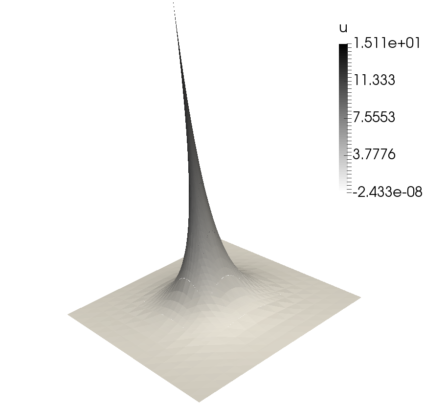
(b)

Figure 1. Left: mesh for the two dimensional approximation at a fixed refinement step. Right: Numerical solution to (74) with $V(x)=-r^{-3/2}$.

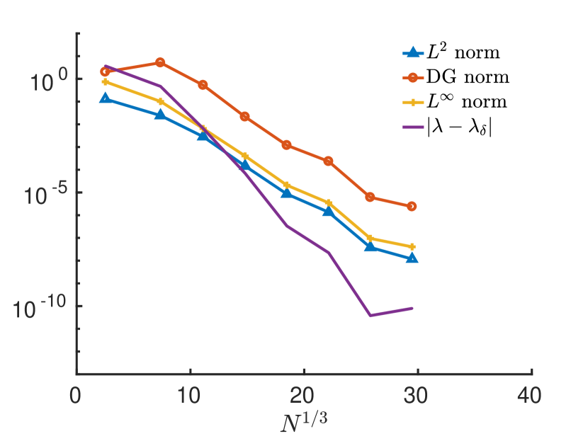
(a)

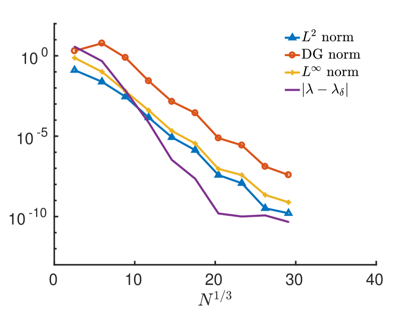
(b)

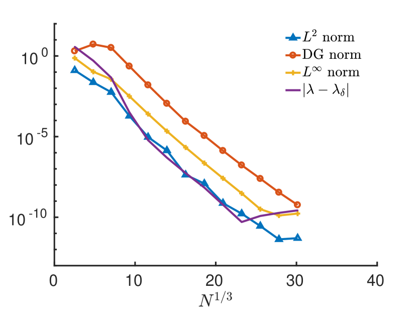
(c)

Figure 2. Estimated errors for the numerical solution with potential $V(x)=-r^{-1/2}$. Polynomial slope: $\mathfrak{s}=1/8$ in Figure 2(a); $\mathfrak{s}=1/4$ in Figure 2(b) and $\mathfrak{s}=1/2$ in Figure 2(c).

Table 1. Estimated coefficients. Potential: $-r^{-1/2}$.

$\mathfrak{s}$		$b_{L^{2}}$		$b_{\mathrm{DG}}$		$b_{L^{\infty}}$		$b_{\lambda}$
$0.125$		$0.72$		$0.73$		$0.74$		$1.24$
$0.25$		$0.92$		$0.94$		$0.94$		$1.5$
$0.5$		$1.06$		$1$		$0.98$		$1.25$

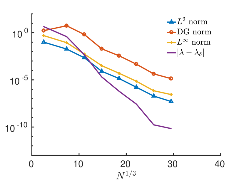
(a)

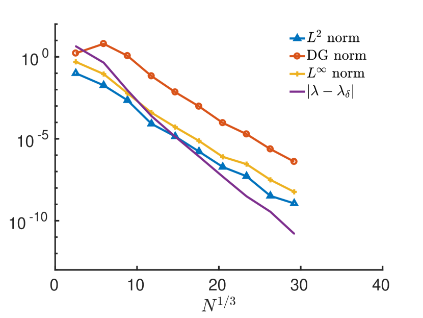
(b)

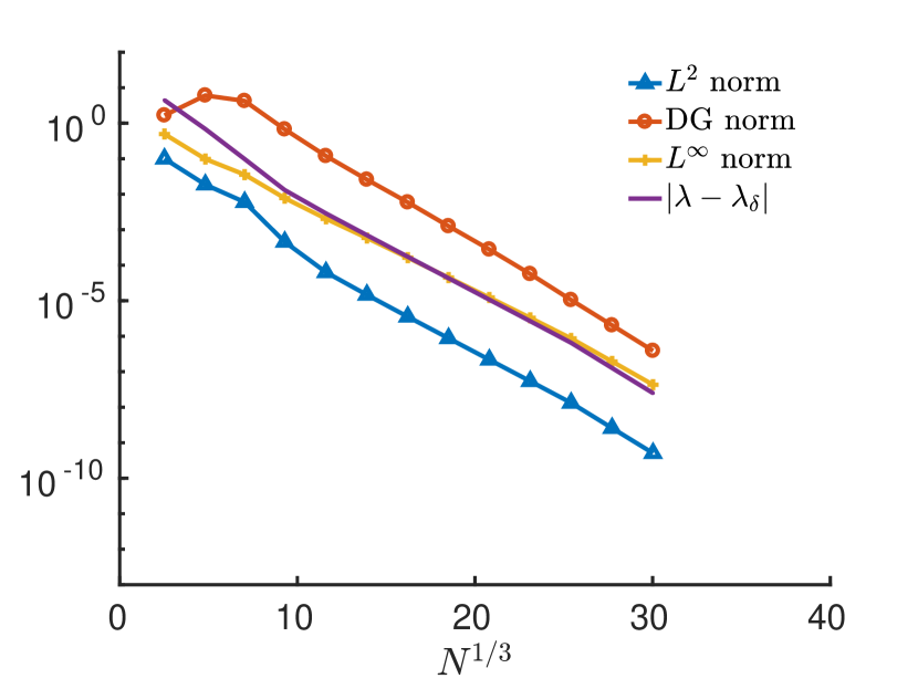
(c)

Figure 3. Estimated errors for the numerical solution with potential $V(x)=-r^{-1}$. Polynomial slope: $\mathfrak{s}=1/8$ in Figure 3(a); $\mathfrak{s}=1/4$ in Figure 3(b) and $\mathfrak{s}=1/2$ in Figure 3(c).

Table 2. Estimated coefficients. Potential: $-r^{-1}$.

$\mathfrak{s}$		$b_{L^{2}}$		$b_{\mathrm{DG}}$		$b_{L^{\infty}}$		$b_{\lambda}$
$0.125$		$0.59$		$0.6$		$0.58$		$1.05$
$0.25$		$0.72$		$0.72$		$0.7$		$1.01$
$0.5$		$0.68$		$0.68$		$0.58$		$0.65$

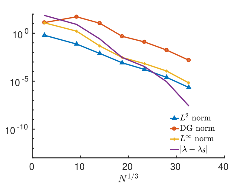
(a)

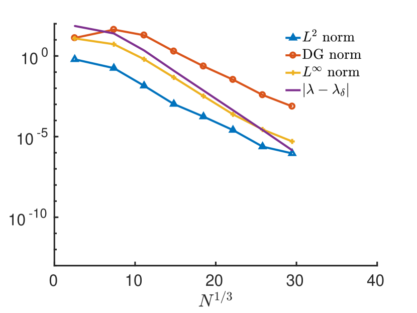
(b)

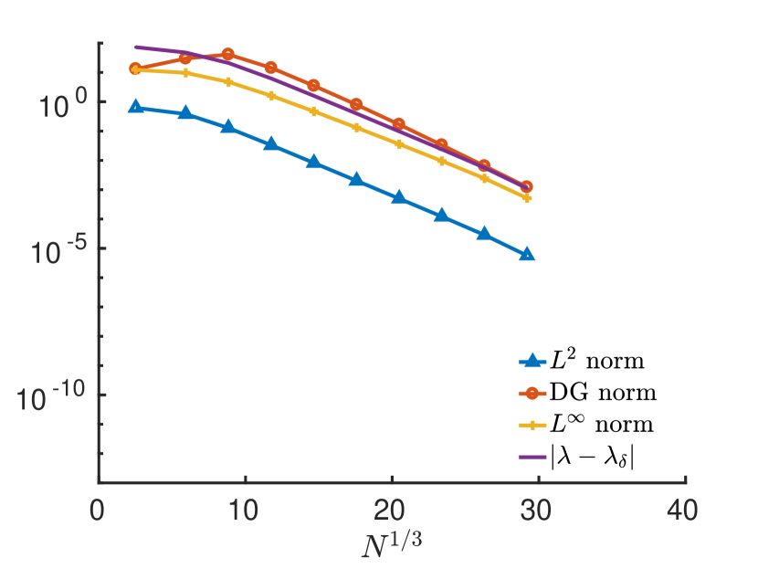
(c)

Figure 4. Estimated errors for the numerical solution with potential $V(x)=-r^{-3/2}$. Polynomial slope: $\mathfrak{s}=1/16$ in Figure 4(a); $\mathfrak{s}=1/8$ in Figure 4(b) and $\mathfrak{s}=1/4$ in Figure 4(c).

Table 3. Estimated coefficients. Potential: $-r^{-3/2}$.

$\mathfrak{s}$		$b_{L^{2}}$		$b_{\mathrm{DG}}$		$b_{L^{\infty}}$		$b_{\lambda}$
$0.062$		$0.43$		$0.45$		$0.5$		$0.8$
$0.125$		$0.56$		$0.52$		$0.65$		$0.76$
$0.25$		$0.48$		$0.47$		$0.43$		$0.47$

In the two dimensional case, we compute the numerical solutions on meshes built with refinement ratio $\sigma=1/2$, see Figure 1(a). A visualization of the solution (in the most singular problem we analyse) is given in Figure 1(b).

Writing $V(x)=-r^{-\alpha}$, we plot the curves of the errors in Figures 2 ($\alpha=1/2$), 3 ($\alpha=1$), and 4 ($\alpha=3/2$). In the case of the approximations with low polynomial slopes, all errors converge exponentially in the number of refinement steps, with the eigenvalue error converging faster than the norms of the eigenfunction error. Estimated errors tend to reach a plateau at values around $10^{-10}$. We conjecture this to be due to algebraic error, as the matrices resulting from the discretization are very ill conditioned for high levels of refinement [2]. A comprehensive study of this effect and of the efficient preconditioning of this problem is out of the scope of the present work. When the polynomial slopes are higher, the quadrature error — not analyzed here, see Ref. [4] for the analysis for $h$-type FE — manifests itself more strongly and causes, in extreme cases, the total loss of the doubling of the convergence rate.

The coefficients $b_{X}$, for $X=L^{2}(\Omega),\mathrm{DG},L^{\infty}(\Omega)$ and $\lambda$ are shown in Tables 1 to 3. As already discussed in Ref. [19], the higher the slope, the biggest the quadrature error and the furthest the estimated coefficients $b_{\lambda}$ is from the double of the one for the $\mathrm{DG}$ norm.

6.1.1. Corner refinement

Since we impose Dirichlet boundary conditions, singularities in the solution can emerge at the corner of the domain. To verify that those potential (milder) singularities do not influence, up to the precision considered, the convergence of the numerical scheme, we perform a comparison between the results with the mesh in Figure 1(a) and a mesh with refinement towards the corners of the domain (see Figure 5(a)). The results are shown in Figure 5 for $\mathfrak{s}=1/2$ and $V(x)=|x|^{-1}$. We compute the errors at the same levels of refinement for corner-refined and non corner-refined meshes and denote by $N_{\mathrm{cor}}$ the number of degrees of freedom of the $hp$ space on the corner-refined mesh and by $N$ the number of degrees of freedom of the space on the mesh without corner refinement. At a given level of refinement, the errors are approximately the same, but since $N_{\mathrm{cor}}\simeq 2N$ the approximation with corner refined mesh is less efficient. This could be related to the superconvergence proved in Ref. [3]. Other choices of slopes and potentials give similar results.

(a)

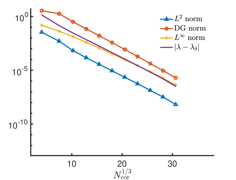
(b)

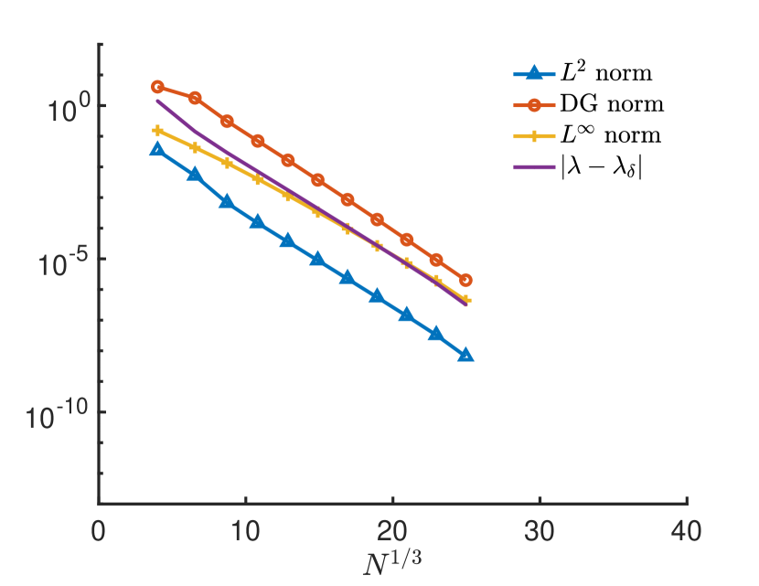
(c)

Figure 5. Top: mesh with corner refinement. Bottom: comparison of results with (left) and without (right) corner refinement.

6.2. Three dimensional problem

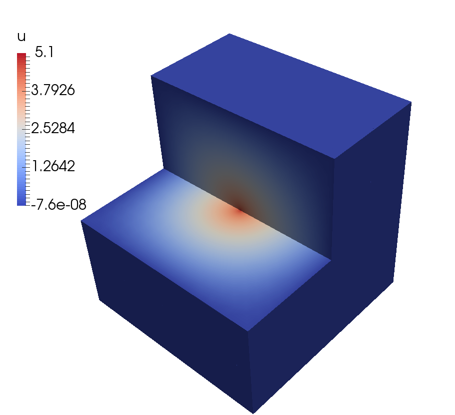
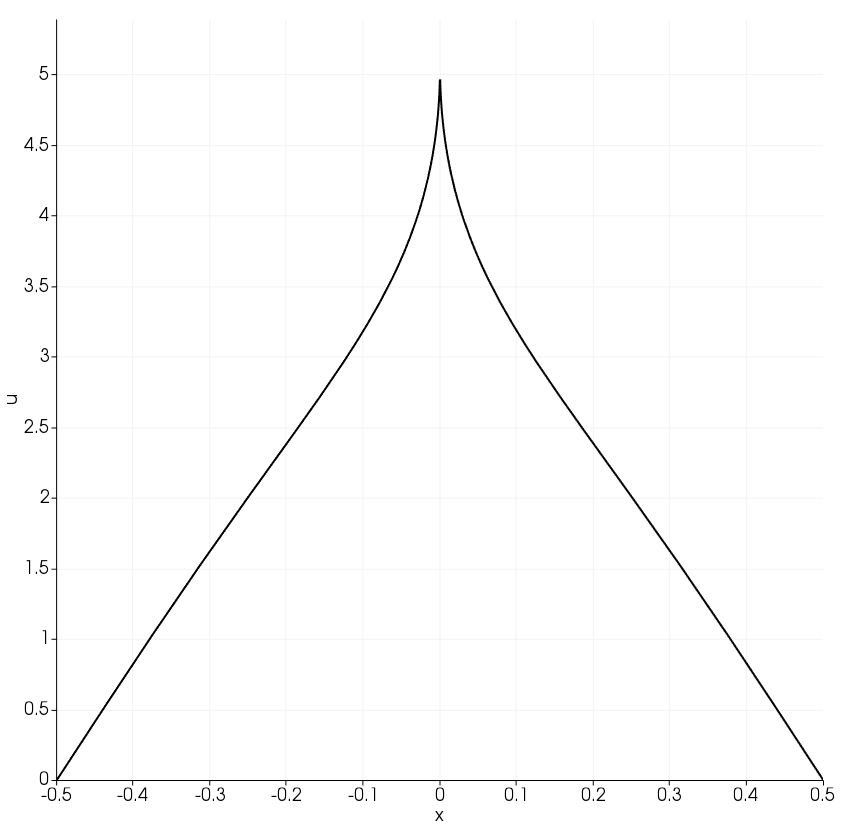
Figure 6. Numerical solution in the three dimensional case: solution in the cube, left, and close up near the origin of the restriction to the line $\{y=z=0\}$, right

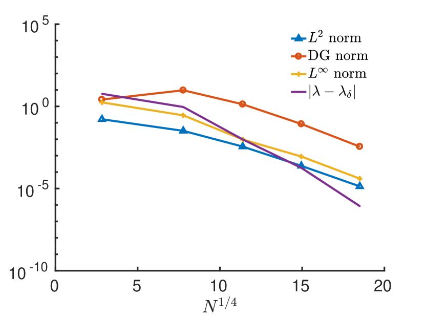
Figure 7. Estimated errors of the numerical solution for $V(x)=r^{-1/2}$. Polynomial slope $\mathfrak{s}=1/8$, left and $\mathfrak{s}=1/4$, right.

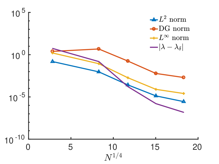
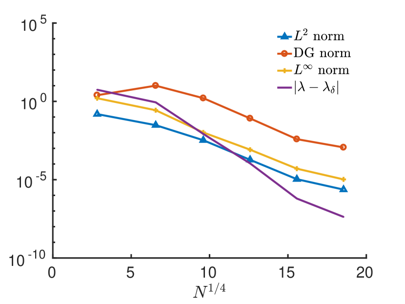
Figure 8. Estimated errors of the numerical solution for $V(x)=r^{-1}$. Polynomial slope $\mathfrak{s}=1/8$, left and $\mathfrak{s}=1/4$, right.

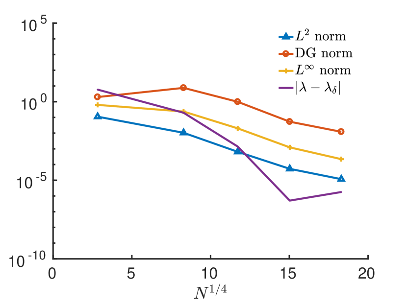
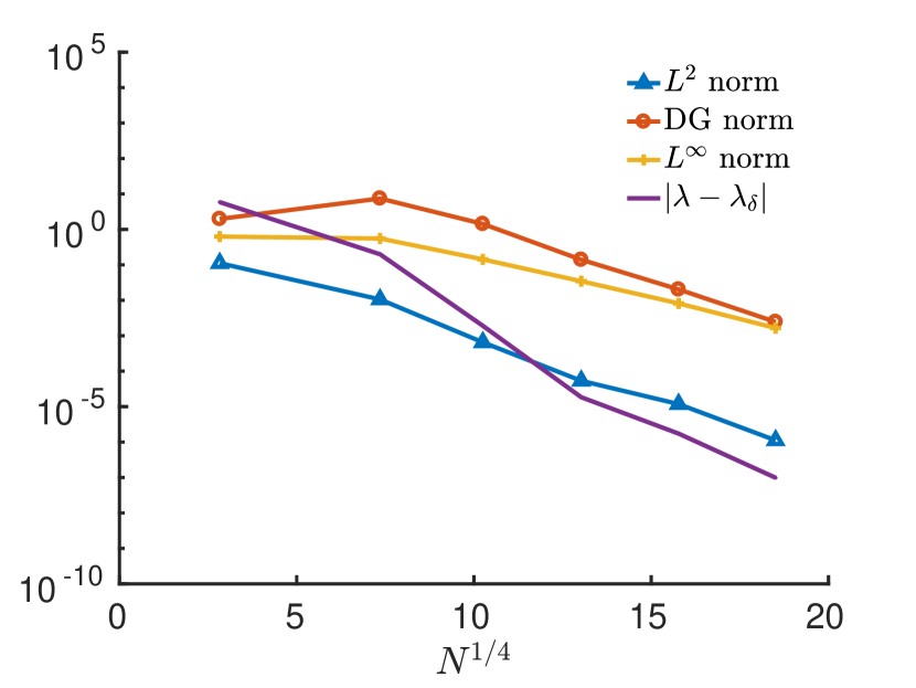
Figure 9. Estimated errors of the numerical solution for $V(x)=r^{-3/2}$. Polynomial slope $\mathfrak{s}=1/8$, left and $\mathfrak{s}=1/4$, right.

Table 4. Estimated coefficients. Potential: $-r^{-1/2}$.

$\mathfrak{s}$		$b_{L^{2}}$		$b_{\mathrm{DG}}$		$b_{L^{\infty}}$		$b_{\lambda}$
$0.125$		$0.73$		$0.74$		$0.81$		$1.28$
$0.25$		$0.82$		$0.82$		$0.85$		$1.3$

Table 5. Estimated coefficients. Potential: $-r^{-1}$.

$\mathfrak{s}$		$b_{L^{2}}$		$b_{\mathrm{DG}}$		$b_{L^{\infty}}$		$b_{\lambda}$
$0.125$		$0.82$		$0.8$		$0.83$		$1.39$
$0.25$		$0.82$		$0.81$		$0.86$		$1.44$

Table 6. Estimated coefficients. Potential: $-r^{-3/2}$.

$\mathfrak{s}$		$b_{L^{2}}$		$b_{\mathrm{DG}}$		$b_{L^{\infty}}$		$b_{\lambda}$
$0.125$		$0.69$		$0.67$		$0.71$		$1.29$
$0.25$		$0.8$		$0.73$		$0.52$		$1.3$

In the three dimensional setting, we consider the domain $(-1/2,1/2)^{3}$, and a mesh exemplified with refinement ratio $\sigma=1/2$. The numerical solution of the problem with $V(x)=r^{-3/2}$ is shown in Figure 6. The solution shown is obtained at one of the highest degrees of refinement. The algebraic eigenproblem solver uses the Jacobi-Davidson method [25], with a biconjugate gradient method [29, 26] as the linear algebraic system solver. The fixed point nonlinear iteration are set to a tolerance $\varepsilon_{\mathrm{tol}}=10^{-7}$.

The algebraic and quadrature errors are not as evident as in the two dimensional case, and it can clearly be seen that an optimal slope can be chosen to better approximate the eigenvalue.

As in the two dimensional case, we expect that corner and edge singularities do not influence the convergence of the method. We do not investigate this further.

The presence of the nonlinearity does not seem to influence the rate of convergence with respect to the rate obtained for the $hp$ dG approximation of linear eigenvalue problem with singular potentials in Ref. [19]. This is expected, as the regularity of the solution of the linear problem considered in Ref. [19] and the regularity of the solution of the problem considered in this section is the same.

References

- [1] P. F. Antonietti, A. Buffa, and I. Perugia, Discontinuous Galerkin approximation of the Laplace eigenproblem, Comput. Methods Appl. Mech. Engrg., 195 (2006), pp. 3483–3503.
- [2] P. F. Antonietti and P. Houston, A class of domain decomposition preconditioners for -discontinuous Galerkin finite element methods, J. Sci. Comput., 46 (2011), pp. 124–149.
- [3] C. Bernardi and Y. Maday, Polynomial approximation of some singular functions, Appl. Anal., 42 (1991), pp. 1–32.
- [4] E. Cancès, R. Chakir, and Y. Maday, Numerical analysis of nonlinear eigenvalue problems, J. Sci. Comput., 45 (2010), pp. 90–117.
- [5] M. Costabel, M. Dauge, and S. Nicaise, Corner singularities and analytic regularity for linear elliptic systems, 2010. Book in preparation.
- [6] , Mellin analysis of weighted Sobolev spaces with nonhomogeneous norms on cones, in Around the research of Vladimir Maz’ya. I, vol. 11 of Int. Math. Ser. (N. Y.), Springer, New York, 2010, pp. 105–136.
- [7] , Analytic regularity for linear elliptic systems in polygons and polyhedra, Math. Models Methods Appl. Sci., 22 (2012), pp. 1250015, 63.
- [8] A. Dall’Acqua, S. Fournais, T. Østergaard Sørensen, and E. Stockmeyer, Real analyticity away from the nucleus of pseudorelativistic Hartree-Fock orbitals, Anal. PDE, 5 (2012), pp. 657–691.
- [9] D. A. Di Pietro and A. Ern, Mathematical aspects of discontinuous Galerkin methods, vol. 69 of Mathématiques & Applications (Berlin) [Mathematics & Applications], Springer, Heidelberg, 2012.
- [10] B. Guo and I. Babuška, The h-p version of the finite element method - Part 1: The basic approximation results, Computational Mechanics, 1 (1986), pp. 21–41.
- [11] , The h-p version of the finite element method - Part 2: General results and applications, Computational Mechanics, 1 (1986), pp. 203–220.
- [12] B. Guo and C. Schwab, Analytic regularity of Stokes flow on polygonal domains in countably weighted Sobolev spaces, J. Comput. Appl. Math., 190 (2006), pp. 487–519.
- [13] K. Kato, New idea for proof of analyticity of solutions to analytic nonlinear elliptic equations, SUT J. Math., 32 (1996), pp. 157–161.
- [14] V. A. Kondrat’ev, Boundary value problems for elliptic equations in domains with conical or angular points, Trudy Moskov. Mat. Obšč., 16 (1967), pp. 209–292.
- [15] V. A. Kozlov, V. Maz’ya, and J. Rossmann, Elliptic boundary value problems in domains with point singularities, vol. 52 of Mathematical Surveys and Monographs, American Mathematical Society, Providence, RI, 1997.
- [16] A. Lasis and E. Suli, Poincaré-type inequalities for broken Sobolev spaces, Tech. Rep. 03/10, Oxford University Computing Laboratory, 2003.
- [17] M. Lewin, Solutions of the multiconfiguration equations in quantum chemistry, Arch. Ration. Mech. Anal., 171 (2004), pp. 83–114.
- [18] H. Liu, Optimal error estimates of the direct discontinuous Galerkin method for convection-diffusion equations, Math. Comp., 84 (2015), pp. 2263–2295.
- [19] Y. Maday and C. Marcati, Regularity and discontinuous Galerkin finite element approximation of linear elliptic eigenvalue problems with singular potentials, Math. Models Methods Appl. Sci., 29 (2019), pp. 1585–1617.
- [20] V. Maz’ya and J. Rossmann, Elliptic equations in polyhedral domains, vol. 162 of Mathematical Surveys and Monographs, American Mathematical Society, Providence, RI, 2010.
- [21] Y. Saad, Numerical methods for large eigenvalue problems, vol. 66 of Classics in Applied Mathematics, Society for Industrial and Applied Mathematics (SIAM), Philadelphia, PA, 2011.
- [22] D. Schötzau, C. Schwab, and T. Wihler, -dGFEM for Second-Order Elliptic Problems in Polyhedra I: Stability on Geometric Meshes, SIAM Journal on Numerical Analysis, 51 (2013), pp. 1610–1633.
- [23] D. Schötzau, C. Schwab, and T. P. Wihler, -DGFEM for second order elliptic problems in polyhedra II: Exponential convergence, SIAM J. Numer. Anal., 51 (2013), pp. 2005–2035.
- [24] K. Shahbazi, An explicit expression for the penalty parameter of the interior penalty method, Journal of Computational Physics, 205 (2005), pp. 401–407.
- [25] G. L. G. Sleijpen and H. A. van der Vorst, A Jacobi-Davidson iteration method for linear eigenvalue problems, SIAM J. Matrix Anal. Appl., 17 (1996), pp. 401–425.
- [26] G. L. G. Sleijpen, H. A. van der Vorst, and D. R. Fokkema, and other hybrid Bi-CG methods, Numer. Algorithms, 7 (1994), pp. 75–109.
- [27] G. Stampacchia, Le problème de Dirichlet pour les équations elliptiques du second ordre à coefficients discontinus, Ann. Inst. Fourier (Grenoble), 15 (1965), pp. 189–258.
- [28] A. Szabo and N. Ostlund, Modern quantum chemistry: introduction to advanced electronic structure theory, Courier Corporation, 2012.
- [29] H. A. van der Vorst, Bi-CGSTAB: a fast and smoothly converging variant of Bi-CG for the solution of nonsymmetric linear systems, SIAM J. Sci. Statist. Comput., 13 (1992), pp. 631–644.
- [30] P. Yin, Y. Huang, and H. Liu, Error estimates for the iterative discontinuous galerkin method to the nonlinear poisson-boltzmann equation, Communications in Computational Physics, 23 (2018), pp. 168–197.