Left-right crossings in the Miller-Abrahams random resistor network and in generalized Boolean models

Abstract.

We consider random graphs $\mathcal{G}$ built on a homogeneous Poisson point process on ${\mathbb{R}}^{d}$, $d\geq 2$, with points $x$ marked by i.i.d. random variables $E_{x}$. Fixed a symmetric function $h(\cdot,\cdot)$, the vertexes of $\mathcal{G}$ are given by points of the Poisson point process, while the edges are given by pairs $\{x,y\}$ with $x\not=y$ and $|x-y|\leq h(E_{x},E_{y})$. We call $\mathcal{G}$ Poisson $h$–generalized Boolean model, as one recovers the standard Poisson Boolean model by taking $h(a,b):=a+b$ and $E_{x}\geq 0$. Under general conditions, we show that in the supercritical phase the maximal number of vertex-disjoint left-right crossings in a box of size $n$ is lower bounded by $Cn^{d-1}$ apart from an event of exponentially small probability. As special applications, when the marks are non-negative, we consider the Poisson Boolean model and its generalization to $h(a,b)=(a+b)^{\gamma}$ with $\gamma>0$, the weight-dependent random connection models with max-kernel and with min-kernel and the graph obtained from the Miller-Abrahams random resistor network in which only filaments with conductivity lower bounded by a fixed positive constant are kept.

Keywords: Poisson point process, Boolean model, Miller–Abrahams random resistor network, left-right crossings, renormalization.

AMS 2010 Subject Classification: 60G55, 82B43, 82D30

1. Introduction

We introduce a random graph $\mathcal{G}$, called Poisson $h$–generalized Boolean model, with vertexes in ${\mathbb{R}}^{d}$ where $d\geq 2$, whose construction depends on a structural symmetric function $h(\cdot,\cdot)$ with real entries, a parameter $\lambda>0$ and a probability measure $\nu$ on ${\mathbb{R}}$. Given a homogeneous Poisson point process (PPP) $\xi$ on ${\mathbb{R}}^{d}$ with intensity $\lambda$, we mark points $x$ of $\xi$ by i.i.d. random variables $E_{x}$ with common distribution $\nu$. Then the vertexes of $\mathcal{G}$ are the points in $\xi$, while edges of $\mathcal{G}$ are given by unordered pairs of vertexes $\{x,y\}$ with $x\not=y$ and $|x-y|\leq h(E_{x},E_{y})$. When $E_{x}\in[1,+\infty)$ and $h(\cdot,\cdot)$ is non–decreasing in each entry, then $\mathcal{G}$ belongs to the class of weight-dependent random connection models introduced in [10].

When $\nu$ has support inside $[0,+\infty)$ and $h(a,b)=a+b$, one recovers the so called Poisson Boolean model [15]. Another relevant example is related to the Miller-Abrahams (MA) random resistor network. This resistor network has been introduced in [16] to study the anomalous conductivity at low temperature in amorphous materials as doped semiconductors, in the regime of Anderson localization and at low density of impurities. It has been further investigated in the physical literature (cf. [2], [17] and references therein), where percolation properties have been heuristically analyzed. A fundamental target has been to get a more robust derivation of the so called Mott’s law, which is a physical law predicting the anomalous decay of electron conductivity at low temperature (cf. [5, 6, 7, 9, 17] and references therein).

When built on a marked PPP $\{(x,E_{x})\,:x\in\xi\}$ as above, the MA random resistor network has nodes given by points in $\xi$ and electrical filaments connecting each pair of nodes. The electrical conductivity of the filament between $x$ and $y$ is given by (cf. [2, Eq. (3.7)])

$$c(x,y):=\exp\Big{\{}-\frac{2}{\gamma}|x-y|-\frac{\beta}{2}(|E_{x}|+|E_{y}|+|E_{x}-E_{y}|)\Big{\}}\,,$$ (1)

where $\beta$ is the inverse temperature and $\gamma$ is the so–called localization length. The physically relevant distributions $\nu$ (for inorganic materials) are of the form $\nu_{\rm phys}(dE)\propto\mathds{1}(|E|\leq a_{0})|E|^{\alpha}dE$ with $\alpha\geq 0$ and $a_{0}>0$.

Note that the conductivity of the filaments is smaller than $1$. Fixed $c_{0}\in(0,1)$, the resistor subnetwork $\mathcal{G}$ given by the filaments with conductivity lower bounded by $c_{0}$ is a Poisson $h$–generalized Boolean model with $h(a,b):=-(\gamma/2)\ln c_{0}-(\gamma\beta/4)(|a|+|b|+|a-b|)$. We point out that, in the low temperature regime (i.e. when $\beta\uparrow\infty$), the conductivity of the MA random resistor network is mainly supported by the subnetwork $\mathcal{G}$ associated to a suitable constant $c_{0}=c_{0}(\beta)$ (cf. [2, 6]). Hence, to shorten the terminology and with a slight abuse, in the rest we call $\mathcal{G}$ itself “MA random resistor network”. Moreover, without loss of generality, we take $\beta=\gamma=2$.

For the supercritical Bernoulli site and bond percolations on ${\mathbb{Z}}^{d}$ with $d\geq 2$, it is known that the maximal number of vertex-disjoint left-right crossings of a box $[-L,L]^{d}$ is lower bounded by $CL^{d-1}$ apart from an event with exponentially small probability (cf. [11, Thm. (7.68), Lemma (11.22)] and [12, Remark (d)]). A similar result is proved for the supercritical Poisson Boolean model with deterministic radius in [18]. Our main result is that, under general suitable conditions, the same behavior holds for the $h$–generalized Boolean model (cf. Theorem 1). This result for the MA random resistor network is relevant when studying the low–temperature conductivity in amorphous solids (cf. [2, 6]).

We comment now some technical aspects in the derivation of our contribution. To prove Theorem 1 we first show that it is enough to derive a similar result (given by Theorem 2 in Section 3) for a suitable random graph ${\mathbb{G}}_{+}$ with vertexes in $\varepsilon{\mathbb{Z}}^{d}$, defined in terms of i.i.d. random variables parametrized by points in $\varepsilon{\mathbb{Z}}^{d}$. The proof of Theorem 2 is then inspired by the renormalization procedure developed by Grimmett and Marstrand in [12] for site percolation on ${\mathbb{Z}}^{d}$ and by a construction presented by Tanemura in [18, Section 4]. We recall that in [12] it is proved that the critical probability of a slab in ${\mathbb{Z}}^{d}$ converges to the critical probability of ${\mathbb{Z}}^{d}$ when the thickness of the slab goes to $+\infty$.

We point out that the renormalization method developed in [12] does not apply verbatim to our case. In particular the adaptation of Lemma 6 in [12] to our setting presents several obstacles due to spatial correlations in our model. A main novelty here is to build, by a Grimmett-Marstrand-like renormalization procedure, an increasing family of quasi-clusters in our graph ${\mathbb{G}}_{+}$. We use here the term “quasi-cluster” since usually these sets are not connected in ${\mathbb{G}}_{+}$ and can present some cuts at suitable localized regions. By expressing the PPP of intensity $\lambda$ as superposition of two independent PPP’s with intensity $\lambda-\delta$ and $\delta\ll 1$, respectively, a quasi-cluster is built only by means of points in the PPP with intensity $\lambda-\delta$. On the other hand, we will show that, with high probability, when superposing the PPP with intensity $\delta$ we will insert a family of points linked with the quasi-cluster, making the resulting set connected in ${\mathbb{G}}_{+}$. This construction relies on the idea of “sprinkling” going back to [1] (see also [11] and references therein).

We remark that in [14] Martineau and Tassion have extended, with some modifications and simplifications, the Grimmett-Marstrand renormalization scheme. Nevertheless, we have followed here the construction in [12] since it is more suited to be combined with Tanemura’s algorithm, which prescribes step by step to build clusters in ${\mathbb{G}}_{+}$ along the axes of ${\mathbb{R}}^{d}$ (while in [14] there is a good building direction, which is not explicit). On the other hand, the fundamental steps in our Grimmett-Marstrand-like renormalization scheme are slightly simplified w.r.t. the original ones in [12].

As special applications of Theorem 1 we consider, for non-negative marks, the cases $h(a,b):=(a+b)^{\gamma}$ with $\gamma>0$, $h(a,b):=\max(a,b)$, $h(a,b):=\min(a,b)$ and $h(a,b):=\zeta-(|a|+|b|+|a-b|)$ with $\zeta>0$ (see Corollaries 2.4 and 2.5). The first case, with $\gamma=1$, generalizes Tanemura’s result to the Poisson Boolean model with random radius. The second and third cases correspond respectively to the min-kernel and the max-kernel random connection model (see [10] and references therein). The fourth case corresponds to the MA random resistor network with non-negative energy marks. Although this result does not cover the mark distributions $\nu_{\rm phys}$ mentioned above, it is suited to distributions $\nu(dE)\propto\mathds{1}(0\leq E\leq a_{0})|E|^{\alpha}dE$ with $\alpha\geq 0$ and $a_{0}>0$, which have similar scaling properties to the physical ones $\nu_{\rm phys}$. We stress that these scaling properties are relevant in the heuristic derivation of Mott’s law as well as in its rigorous analysis [4, 6]. The restriction to non-negative marks in the MA random resistor network comes from the fact that the Grimmett-Marstrand method (as well as its extension in [14]) relies on the FKG inequality. As one can check, when considering the MA random resistor network with marks having different signs, the FKG inequality can fail.

For the reader’s convenience, an outline of the paper is provided in Section 2.1 after the presentation of models and main results. Finally, we point out that percolation results for the subcritical MA random resistor network have been obtained in [8].

2. Model and main results

We introduce a class of random graphs built by means of a symmetric structural function

$$h:\Delta\times\Delta\to{\mathbb{R}}\,,\qquad\Delta\subset{\mathbb{R}}\,.$$ (2)

To this aim we call $\Omega$ the space of locally finite sets of marked points in ${\mathbb{R}}^{d}$, $d\geq 2$, with marks in $\Delta$. More precisely, a generic element $\omega\in\Omega$ has the form $\omega=\{(x,E_{x})\,:\,x\in\xi\}$, where $\xi$ is a locally finite subset of ${\mathbb{R}}^{d}$ and $E_{x}\in\Delta$ for any $x\in\xi$ ($E_{x}$ is thought of as the mark of point $x$). It is standard (cf. [3]) to define on $\Omega$ a distance such that the $\sigma$–algebra of Borel sets $\mathcal{B}$ of $\Omega$ is generated by the sets $\{|\omega\cap A|=n\}$, $A$ varying among the Borel subsets of ${\mathbb{R}}^{d}$ and $n$ varying in ${\mathbb{N}}$. We assume that $(\Omega,\mathcal{B})$ is endowed with a probability measure $P$, thus defining a marked simple point process.

Definition 2.1 (Graph $\mathcal{G}[\omega]$).

To each $\omega=\{(x,E_{x})\,:\,x\in\xi\}$ in $\Omega$ we associate the unoriented graph $\mathcal{G}[\omega]=\bigl{(}\mathcal{V}[\omega],\mathcal{E}[\omega]\bigr{)}$ with vertex set $\mathcal{V}[\omega]:=\xi$ and edge set $\mathcal{E}[\omega]$ given by the unordered pairs $\{x,y\}$ with $x\not=y$ in $\xi$ and

$$|x-y|\leq h(E_{x},E_{y})\,.$$ (3)

We call $h$–generalized Boolean model the resulting random graph $\mathcal{G}=\mathcal{G}[\omega]$ defined on $(\Omega,\mathcal{B},P)$.

When $\Delta:={\mathbb{R}}_{+}$ and $h(a,b):=a+b$, one has indeed the so–called Boolean model [15]. As discussed in the Introduction, another relevant example is given by the MA random resistor network with lower bounded conductances: in this case $\Delta={\mathbb{R}}$ and, fixed the parameter $\zeta>0$, the structural function $h:{\mathbb{R}}\times{\mathbb{R}}\to{\mathbb{R}}$ is given by

$$h(a,b):=\zeta-\bigl{(}|a|+|b|+|a-b|\bigr{)}\,.$$ (4)

We focus here on the left-right crossings of the graph $\mathcal{G}=\mathcal{G}[\omega]$:

Definition 2.2 (LR crossing and $\mathcal{R}_{L}(\mathcal{G})$).

Given $L\in(0,+\infty)$, a left-right (LR) crossing of the box $[-L,L]^{d}$ in the graph $\mathcal{G}$ is any sequence of distinct points $x_{1},x_{2},\dots,x_{n}\in\xi$ such that

• $\{x_{i},x_{i+1}\}\in\mathcal{E}$ for all $i=1,2,\dots,n-1$;

• $x_{1}\in(-\infty,-L)\times[-L,L]^{d-1}$;

• $x_{2},x_{3},\dots,x_{n-1}\in[-L,L]^{d}$;

• $x_{n}\in(L,+\infty)\times[-L,L]^{d-1}$.

We also define $\mathcal{R}_{L}(\mathcal{G})$ as the maximal number of vertex-disjoint LR crossings of $[-L,L]^{d}$ in $\mathcal{G}$.

In what follows, given $\lambda>0$ and a probability measure $\nu$ with support contained in $\Delta$, we consider the marked Poisson point process (PPP) obtained by sampling $\xi$ according to a homogeneous PPP with intensity $\lambda$ on ${\mathbb{R}}^{d}$ ($d\geq 2$) and marking each point $x\in\xi$ independently with a random variable $E_{x}$ having distribution $\nu$ (conditioning to $\xi$, the marks $(E_{x})_{x\in\xi}$ are i.i.d. random variables with distribution $\nu$). The above marked point process is called $\nu$-randomization of the PPP with intensity $\lambda$ (cf. [13, Chp. 12]). The resulting random graph $\mathcal{G}$, whose construction depends also on the structural function $h$, will be denoted by $\mathcal{G}(h,\lambda)=\mathcal{G}(h,\lambda)[\omega]$ when necessary (note that $\nu$ is understood).

To state our main assumptions, we recall that, given a generic graph with vertexes in ${\mathbb{R}}^{d}$, one says that it percolates if it has an unbounded connected component. We also fix, once and for all, a constant $\lambda>0$ and a probability measure $\nu$ on $\Delta$. We write ${\rm supp}(\nu)$ for the support of $\nu$.

Assumptions:

• $P$ is the $\nu$–randomization of a PPP with intensity $\lambda$ on ${\mathbb{R}}^{d}$, $d\geq 2$.

• There exist $\lambda_{*}<\lambda$ and $\ell_{*}>0$ such that $\mathcal{G}(h-\ell_{*},\lambda_{*})$ percolates a.s..

• $\sup\left\{h(a,b)\,:\,a,b\in\text{supp}(\nu)\right\}\in(0,+\infty)$.

• For any $\delta>0$ there exists a Borel subset $U_{*}(\delta)\subset\Delta$ with $\nu(U_{*}(\delta))>0$ such that

  $$\inf_{a\in U_{*}(\delta)}h(a,b)\geq\sup_{a^{\prime}\in{\rm supp}(\nu)}h(a^{\prime},b)-\delta\,,\qquad\forall b\in{\rm supp}(\nu)\,.$$ (5)

• As $a,b$ vary in ${\rm supp}(\nu)$, $h(a,b)$ is weakly decreasing both in $a$ and in $b$ (shortly, $h\searrow$), or $h(a,b)$ is weakly increasing both in $a$ and in $b$ (shortly, $h\nearrow$).

Let us comment our assumptions.

The definition of $h$ is relevant only for entries in ${\rm supp(\nu)}$, hence one could as well restrict to the case $\Delta={\rm supp}(\nu)$. Since the $h$–generalized Boolean model presents spatial correlations by its own definition, Assumptions (A1) avoids further spatial correlations inherited from the marked point process.

By a simple coupling argument, (A2) implies that $\mathcal{G}(h-\ell^{\prime},\lambda^{\prime})$ percolates a.s. for any $\ell^{\prime}\in[0,\ell_{*}]$ and $\lambda^{\prime}\in[\lambda_{*},\lambda]$. Hence, (A2) assures some form of “stable supercriticality” of the graph $\mathcal{G}(h,\lambda)$.

Due to (3), (A3) both excludes the trivial case $h\leq 0$ on ${\rm supp}(\nu)$ (which would imply that $\mathcal{G}(h,\lambda)$ has no edges) and guarantees that the length of the edges of $\mathcal{G}(h,\lambda)$ is a.s. bounded by some deterministic constant.

We move to (A4). By definition of supremum and due to (A3), for any $\delta>0$ and for any $b\in{\rm supp}(\nu)$ there exists $a\in{\rm supp}(\nu)$ such that $h(a,b)\geq\sup_{a^{\prime}\in{\rm supp}(\nu)}h(a,b)-\delta$. Assumption (A4) enforces this free inequality requiring that it is satisfies uniformly in $a$ varying in some subset $U_{*}(\delta)$ with positive $\nu$–measure. For example, if $h$ is continuous, ${\rm supp}(\nu)$ is bounded and (A5) is satisfied, then (A4) is automatically satisfied. Indeed, if e.g. $h\nearrow$, then $\sup_{a^{\prime}\in{\rm supp}(\nu)}h(a^{\prime},b)=h(A,b)$ with $A:=\max\bigl{(}\text{supp}(\nu)\bigr{)}$ and the claim follows by uniform continuity.

We move to (A5). This assumption implies that we enlarge the graph when reducing the marks if $h\searrow$ or increasing the marks if $h\nearrow$. Moreover, (A5) guarantees the validity of the FKG inequality (cf. Section 3.1), which in general can fail.

Our main result is the following one:

Theorem 1.

Suppose that the intensity $\lambda>0$ and the mark probability distribution $\nu$ satisfy the above Assumptions (A1),…,(A5). Then there exist positive constants $c,c^{\prime}$ such that

$$P\left({\color[rgb]{0,0,0}\mathcal{R}_{L}(\mathcal{G})}\geq cL^{d-1}\right)\geq 1-e^{-c^{\prime}L^{d-1}}\,,$$ (6)

for $L$ large enough, where $\mathcal{G}=\mathcal{G}(h,\lambda)$.

The proof of Theorem 1 is localized as follows: by Proposition 3.5 to get Theorem 1 it is enough to prove Theorem 2. By Proposition 3.6 to get Theorem 2 it is enough to prove (25) in Proposition 3.6. The proof of (25) in Proposition 3.6 is given in Section 5.

Remark 2.3.

We point out that (6) cannot hold for all $L>0$, but fixed $L_{0}>0$ one can play with the constants $c,c^{\prime}>0$ to extend (6) to all $L\geq L_{0}$. Let us explain this issue. Calling $\ell_{0}$ the supremum in (A3), we get that all edges of $\mathcal{G}$ have length at most $\ell_{0}$. The event in the l.h.s. of (6) implies that $\mathcal{R}_{L}(\mathcal{G})\geq 1$ and therefore the PPP must contain some point both in $[-L-\ell_{0},-L)\times[-L,L]^{d-1}$ and in $(L,L+\ell_{0}]\times[-L,L]^{d-1}$. Hence the probability in (6) is upper bounded by $(1-e^{-\lambda\ell_{0}(2L)^{d-1}})^{2}$, which is of order $L^{2d-2}$ as $L\downarrow 0$. As $d\geq 2$ we conclude that (6) cannot hold for $L$ too small. On the other hand, fix $L_{0}>0$ and suppose that (6) holds for all $L\geq L_{1}$ for some $L_{1}>L_{0}$. Take now $L\in[L_{0},L_{1}]$. Our assumptions imply that there exists a set $W\subset{\mathbb{R}}$ such that $\nu(W)>0$ and $r:=\inf_{a,b\in W}h(a,b)>0$ (cf. (37)). Set $e_{1}:=(1,0,\dots,0)$, $\ell:=\min(r,L_{0})$ and let $N$ be the minimal positive integer such that $N\ell/2>L_{1}$. Then $\mathcal{R}_{L}(\mathcal{G})\geq 1$ whenever each ball of radius $\ell/10$ and centered at $k(\ell/2)e_{1}$ contains some point $x$ of the Poisson process with mark $E_{x}\in W$, where $k$ varies from $-N-1$ to $N+1$. Note that this last event does not depend on $L$, and therefore the same holds for its positive probability. At this point, by playing with $c,c^{\prime}$ in (6), one can easily extend (6) to all $L\geq L_{0}$.

We now discuss some applications.

Let $d\geq 2$, $\lambda>0$ and let $h:{\mathbb{R}}_{+}\times{\mathbb{R}}_{+}\rightarrow{\mathbb{R}}$ be one of the following functions (for the first one $\gamma$ is a fixed positive constant):

$$h(a,b):=(a+b)^{\gamma}\,,\qquad h(a,b):=\min(a,b)\,\qquad h(a,b):=\max(a,b)\,.$$ (7)

Consider the graph $\mathcal{G}=\mathcal{G}(h,\lambda)$ built on the $\nu$–randomization of a PPP on ${\mathbb{R}}^{d}$ with intensity $\lambda$. As proved in Section 8 (cf. Lemma 8.1), if $\nu$ has bounded support and $\nu(\{0\})\not=1$, then there exists a critical intensity $\lambda_{c}$ in $(0,+\infty)$ such that

$$P\bigl{(}\mathcal{G}\text{ percolates})=\begin{cases}1&\text{ if }\lambda>\lambda_{c}\,,\\ 0&\text{ if }\lambda<\lambda_{c}\,.\end{cases}$$ (8)

Corollary 2.4.

Let $d\geq 2$ and let $h$ be given by one of the functions in (7). Consider the graph $\mathcal{G}=\mathcal{G}(h,\lambda)$ built on the $\nu$–randomization of a PPP on ${\mathbb{R}}^{d}$ with intensity $\lambda>\lambda_{c}$, where the law $\nu$ has bounded support and $\nu(\{0\})\not=1$. Then there exist $c,c^{\prime}>0$ such that (6) is fulfilled for $L$ large enough.

We postpone the proof of the above corollary to Section 8. Note that we recover the Poisson Boolean model [15] when $h(a,b):=(a+b)^{\gamma}$ and $\gamma=1$. We point out that, according to the notation in [10], the above graph $\mathcal{G}(h,\lambda)$ corresponds to the min-kernel (or max-kernel) weight–dependent random connection model by taking $h(a,b)=\max(a,b)$ (respectively $h(a,b)=\min(a,b)$) and by defining the weight of the point $x$ as a suitable rescaling of our $E_{x}$.

Let now $d\geq 2$ and $\zeta,\lambda>0$. Consider the MA random resistor network $\mathcal{G}=\mathcal{G}(h,\lambda)$ with parameter $\zeta$ (i.e. with structural function $h$ given by (4)), built on the $\nu$–randomization of a PPP on ${\mathbb{R}}^{d}$ with intensity $\lambda$. When $\nu$ has bounded support it is trivial to check that there exists a critical length $\zeta_{c}$ in $(0,+\infty)$ such that

$$P\bigl{(}\mathcal{G}\text{ percolates})=\begin{cases}1&\text{ if }\zeta>\zeta_{c}\,,\\ 0&\text{ if }\zeta<\zeta_{c}\,.\end{cases}$$ (9)

Indeed, if $\nu$ has support in $[-A,A]$, then $\mathcal{G}$ contains (is contained in) a random graph distributed as a Poisson Boolean model with intensity $\lambda$ and deterministic radius $\zeta/2-2A$ ($\zeta/2$ respectively). Equivalently, one could keep $\zeta$ fixed and play with the intensity $\lambda$ getting a phase transition as in (8) under suitable assumptions (see [8, Prop. 2.2]). For physical reasons it is more natural to vary $\zeta$ while keeping $\lambda$ fixed. Then we have:

Corollary 2.5.

Let $d\geq 2$ and $\lambda>0$. Consider the MA random resistor network with parameter $\zeta>\zeta_{c}$ built on the $\nu$–randomization of a PPP on ${\mathbb{R}}^{d}$ with intensity $\lambda$. Suppose that $\nu$ has bounded support contained in $[0,+\infty)$ or in $(-\infty,0]$. Then there exist positive constants $c,c^{\prime}$ such that (6) is satisfied for $L$ large enough.

We postpone the proof of the above corollary to Section 8. We point out that given $a,b\in{\mathbb{R}}$, it holds

$$|a|+|b|+|a-b|=\begin{cases}2\max\bigl{(}|a|,|b|\bigr{)}&\text{ if }ab\geq 0\,,\\ 2|a-b|&\text{ if }ab<0\,.\end{cases}$$ (10)

Hence, the structural function $h$ defined by (4) reads $h(a,b)=\zeta-2\max(|a|,|b|)$ if $ab\geq 0$, and $h(a,b)=\zeta-2|a-b|$ if $ab<0$. As a consequence, if the support of $\nu$ intersects both $(-\infty,0)$ and $(0,\infty)$, then Assumption (A5) fails.

2.1. Outline of the paper

The proof of Theorem 1 consists of two main steps: 1) reduction to the analysis of the LR crossings inside a 2d slice of a suitable graph approximating $\mathcal{G}$ and having vertexes in a lattice, 2) combination of Tanemura’s algorithm in [18, Section 4.1] and Grimmett-Marstrand renormalization scheme in [12] to perform the above reduced analysis.

For what concerns the first part, in Section 3 we show that it is enough to prove the analogous of Theorem 1 for a suitable graph ${\mathbb{G}}_{+}$ whose vertexes lie inside $\varepsilon{\mathbb{Z}}^{d}$, with $\varepsilon>0$ small enough. By a standard argument (cf. [12, Remark (d)]), we then show that it is indeed enough to have a good control from below of the number of vertex–disjoint LR crossings of ${\mathbb{G}}_{+}$ contained in a 2d slice (this control is analogous to (6) for $d=2$, cf. Eq. (25)).

We then move to the second part. In Section 4 we recall (with some extension) Tanemura’s algorithm in [18] to exhibit a maximal set of vertex-disjoint LR crossings for a generic subgraph of ${\mathbb{Z}}^{2}$, where edges are given by pairs of nearest–neighbor points. Under suitable conditions on the random subgraph of ${\mathbb{Z}}^{2}$, this algorithm allows to stochastically dominate the maximal number of the vertex-disjoint LR crossings by the analogous quantity for a site percolation. If the latter is supercritical, then one gets an estimate for the random subgraph of ${\mathbb{Z}}^{2}$ as (25). We then apply Tanemura’s results by taking as random subgraph of ${\mathbb{Z}}^{2}$ a suitable graph built from ${\mathbb{G}}_{+}$ by a renormalization procedure similar to the one developed by Grimmett & Mastrand in [12]. The combination of the two methods to conclude the proof of the bound (25), and hence of Theorem 1, is provided in Section 5, where the renormalization scheme and its main properties are only roughly described. A detailed treatment of the renormalization scheme is given in Sections 6 and 7.

For the reader’s convenience, in order to allow a better comprehension of the main structure of the proof of Theorem 1, we have postponed several technical proofs in the last sections (see Sections 9, 10, 11, 12). Corollaries 2.4 and 2.5 are proven in Section 8.

Finally, in Appendix A we illustrate Tanemura’s algorithm in a specific example and in Appendix B we collect some straightforward but cumbersome geometric bounds used in the renormalization scheme. In Appendix C we gather some technical arguments for the proof of (25).

3. Discretization and reduction to 2d slices

Warning 3.1.

Without loss of generality we take $\Delta={\rm supp}(\nu)$ and assume that $\sup_{a,b\in\Delta}h(a,b)=1$ (cf. (A3)). In particular, a.s. the length of the edges of $\mathcal{G}$ will be bounded by $1$.

In this section we show how to reduce the problem of estimating the probability $P\left({\color[rgb]{0,0,0}\mathcal{R}_{L}(\mathcal{G})}\geq cL^{d-1}\right)$ in (6) to a similar problem for a graph ${\mathbb{G}}_{+}$ with vertexes contained in the rescaled lattice $\varepsilon{\mathbb{Z}}^{d}$. Afterwards, we show that, for the second problem, it is enough to have a good control on the LR crossings of ${\mathbb{G}}_{+}$ contained in 2d slices.

We need to introduce some notation since we will deal with several couplings:

• We write PPP($\rho$) for the Poisson point process with intensity $\rho$.

• We write PPP($\rho,\nu$) for the marked PPP obtained as $\nu$–randomization of a PPP($\rho$).

• Given a sequence of i.i.d. random variables $(X_{n})_{n\geq 1}$ with law $\nu$ and, independently, a Poisson random variable $N$ with parameter $\rho$, we write $\mathcal{L}(\rho,\nu)$ for the law of $\inf\{X_{1},X_{2},\dots,X_{N}\}$ if $h\searrow$ and the law of $\sup\{X_{1},X_{2},\dots,X_{N}\}$ if $h\nearrow$. When $N=0$, the set $\{X_{1},X_{2},\dots,X_{N}\}$ is given by $\emptyset$ and we use the convention that $\inf\emptyset:=+\infty$ and $\sup\emptyset:=-\infty$.

Recall the constants $\lambda_{*},\ell_{*}$ appearing in Assumption (A2) and the set $U_{*}(\delta)$ appearing in Assumption (A4).

Definition 3.1 (Parameters $\alpha,\varepsilon,K$, set $U_{*}$ and boxes $R_{z}$’s).

We fix a constant $\alpha>0$ small enough such that $10\alpha\leq\ell_{*}$, $10\alpha\leq 1$ and $\sqrt{d}/\alpha\in{\mathbb{N}}_{+}$. We define $\varepsilon$ by $\varepsilon\sqrt{d}:=\alpha/100$ (note that $1/\varepsilon\in{\mathbb{N}}_{+}$). For each $z\in\varepsilon{\mathbb{Z}}^{d}$ we set $R_{z}:=z+[0,\varepsilon)^{d}$. We fix a positive integer $K$, very large. In Section 7.5 we will explain how to choose $K$. Finally, we set $U_{*}:=U_{*}(\alpha/2)$.

Definition 3.2 (Fields $(A_{z})$, $(T^{(j)}_{z})$ and $(A_{z}^{\rm au})$).

We introduce the following $K+1$ independent random fields defined on a common probability space $(\Theta,{\mathbb{P}})$:

• Let $(A_{z})_{z\in\varepsilon{\mathbb{Z}}^{d}}$ be i.i.d. random variables with law $\mathcal{L}\bigl{(}\lambda_{*}\varepsilon^{d},\nu\bigr{)}$.

• Given $j\in\{1,2,\dots,K\}$, let $(T^{(j)}_{z})_{z\in\varepsilon{\mathbb{Z}}^{d}}$ be i.i.d. random variables with law $\mathcal{L}\bigl{(}(\lambda-\lambda_{*})\varepsilon^{d}/K,\nu\bigr{)}$.

By means of the above fields we build an augmented random field given by the i.i.d. random variables $(A_{z}^{\rm au})_{z\in\varepsilon{\mathbb{Z}}^{d}}$, where

$$A_{z}^{\rm au}:=\begin{cases}A_{z}\wedge\min_{1\leq j\leq K}T_{z}^{(j)}&\text{ if }h\searrow\\ A_{z}\lor\max_{1\leq j\leq K}T_{z}^{(j)}&\text{ if }h\nearrow\end{cases}\quad\,.$$ (11)

Note that $A_{z}$ and $A_{z}^{\rm au}$ have value in $\Delta\cup\{+\infty\}$ if $h\searrow$, and in $\Delta\cup\{-\infty\}$ if $h\nearrow$. Let us clarify the relation of the random fields introduced in Definition 3.2 with the PPP$(\lambda,\nu)$. We observe that a PPP$(\lambda,\nu)$ can be obtained as follows. Let

$$\{(x,E_{x})\,:\,x\in\sigma\}\,,$$ (12)

$$\{(x,E_{x})\,:\,x\in\xi^{(j)}\}\qquad j=1,2,\dots,K\,,$$ (13)

be independent marked PPP’s, respectively with law PPP$(\lambda_{*},\nu)$ and PPP$((\lambda-\lambda_{*})/K,\nu)$. In particular, the random sets $\sigma$ and $\xi^{(j)}$, with $1\leq j\leq K$, are a.s. disjoint and correspond to PPP’s with intensity $\lambda_{*}$ and $(\lambda-\lambda_{*})/K$ respectively. The number of points in $\sigma\cap R_{z}$ (respectively $\xi^{(j)}\cap R_{z}$) is a Poisson random variable with parameter $\lambda_{*}\varepsilon^{d}$ (respectively $(\lambda-\lambda_{*})\varepsilon^{d}/K$). Then, setting $\xi:=\sigma\cup\bigl{(}\cup_{j=1}^{K}\xi^{(j)}\bigr{)}$, the marked point process $\{(x,E_{x})\,:\,x\in\xi\}$ is a PPP$(\lambda,\nu)$. Let us first suppose that $h\searrow$. We define

$$B_{z} :=\inf\{E_{x}\,:\,x\in\sigma\cap R_{z}\}\,,\qquad\;\;\;z\in\varepsilon{\mathbb{Z}}^{d}\,,$$ (14)

$$B_{z}^{(j)} :=\inf\{E_{x}\,:\,x\in\xi^{(j)}\cap R_{z}\}\,,\qquad z\in\varepsilon{\mathbb{Z}}^{d}\,,\;j=1,2,\dots,K\,.$$ (15)

Trivially, we have

$$B_{z}^{\rm au}:=B_{z}\wedge\min_{1\leq j\leq K}B_{z}^{(j)}=\inf\{E_{x}\,:\,x\in\xi\cap R_{z}\}\,,\qquad z\in\varepsilon{\mathbb{Z}}^{d}\,.$$ (16)

The above fields in (14) and (15) are independent (also varying $j$) and moreover we have the following identities between laws:

$$\left(B_{z}\right)_{z\in\varepsilon{\mathbb{Z}}^{d}}\stackrel{{\scriptstyle\mathcal{L}}}{{=}}\left(A_{z}\right)_{z\in\varepsilon{\mathbb{Z}}^{d}}\,,$$ (17)

$$\left(B^{(j)}_{z}\right)_{z\in\varepsilon{\mathbb{Z}}^{d}}\stackrel{{\scriptstyle\mathcal{L}}}{{=}}\left(T^{(j)}_{z}\right)_{z\in\varepsilon{\mathbb{Z}}^{d}}\text{ for }j=1,2,\dots,K\,,$$ (18)

$$\left(B_{z}^{\rm au}\right)_{z\in\varepsilon{\mathbb{Z}}^{d}}\stackrel{{\scriptstyle\mathcal{L}}}{{=}}\left(A_{z}^{\rm au}\right)_{z\in\varepsilon{\mathbb{Z}}^{d}}\,.$$ (19)

When $h\nearrow$ the above observations remain valid by replacing $\inf,\min$ with $\sup,\max$, respectively.

Definition 3.3 (Graph ${\mathbb{G}}_{+}=({\mathbb{V}}_{+},{\mathbb{E}}_{+})$).

On the probability space $(\Theta,{\mathbb{P}})$ we define the graph ${\mathbb{G}}_{+}=({\mathbb{V}}_{+},{\mathbb{E}}_{+})$ as

$${\mathbb{V}}_{+} :=\{z\in\varepsilon{\mathbb{Z}}^{d}\,:\,A^{\rm au}_{z}\in{\mathbb{R}}\}\,,$$ (20)

$${\mathbb{E}}_{+} :=\left\{\{z,z^{\prime}\}:z\not=z^{\prime}\text{ in }{\mathbb{V}}_{+}\,,\;\;\;|z-z^{\prime}|\leq h(A^{\rm au}_{z},A^{\rm au}_{z^{\prime}})-\alpha\right\}\,.$$ (21)

The plus suffix comes from the fact that in Sections 3.1 and 6 we will introduce two other graphs, ${\mathbb{G}}_{-},$ and ${\mathbb{G}}$ respectively, such that ${\mathbb{G}}_{-}\subset{\mathbb{G}}\subset{\mathbb{G}}_{+}$.

Definition 3.4 (LR crossing in ${\mathbb{G}}_{+}$ and ${\mathbb{R}}_{L}({\mathbb{G}}_{+})$).

Given $L>0$, a left-right (LR) crossing of the box $\Delta_{L}:=[-L-2,L+2]\times[-L,L]^{d-1}$ in the graph ${\mathbb{G}}_{+}$ is any sequence of distinct vertexes $x_{1},x_{2},\dots,x_{n}$ of ${\mathbb{G}}_{+}$ such that

• $\{x_{i},x_{i+1}\}\in{\mathbb{E}}_{+}$ for all $i=1,2,\dots,n-1$;

• $x_{1}\in(-\infty,-L-2)\times[-L,L]^{d-1}$;

• $x_{2},x_{3},\dots,x_{n-1}\in\Delta_{L}$;

• $x_{n}\in(L+2,+\infty)\times[-L,L]^{d-1}$.

We also define ${\mathbb{R}}_{L}({\mathbb{G}}_{+})$ as the maximal number of vertex-disjoint LR crossings of $\Delta_{L}$ in ${\mathbb{G}}_{+}$.

Theorem 2.

Let ${\mathbb{G}}_{+}$ be the random graph given in Definition 3.3. Then there exist positive constants $c,c^{\prime}$ such that

$${\mathbb{P}}\left({\mathbb{R}}_{L}({\mathbb{G}}_{+})\geq cL^{d-1}\right)\geq 1-e^{-c^{\prime}L^{d-1}}$$ (22)

for $L$ large enough.

To get Theorem 1 it is enough to prove Theorem 2:

Proposition 3.5.

Theorem 2 implies Theorem 1.

Proof.

We restrict to the case $h\searrow$ as the case $h\nearrow$ can be treated by similar arguments. By the above discussion concerning (14), (15) and (16), ${\mathbb{G}}_{+}$ has the same law of the following graph $\bar{\mathbb{G}}_{+}$ built in terms of the random field (16). The vertex set of $\bar{\mathbb{G}}_{+}$ is given by $\{z\in\varepsilon{\mathbb{Z}}^{d}\,:\,B^{\rm au}_{z}<+\infty\}$. The edges of $\bar{\mathbb{G}}_{+}$ are given by the unordered pairs $\{z,z^{\prime}\}$ with $z\not=z^{\prime}$ in the vertex set and

$$|z-z^{\prime}|\leq h(B_{z}^{\rm au},B_{z^{\prime}}^{\rm au})-\alpha\,.$$ (23)

Due to (16) for each vertex $z$ of $\bar{\mathbb{G}}_{+}$ we can fix a point $x(z)\in\xi\cap R_{z}$ such that $E_{x(z)}=B^{\rm au}_{z}$. Hence, if $\{z,z^{\prime}\}$ is an edge of $\bar{\mathbb{G}}_{+}$, then $x(z)$ and $x(z^{\prime})$ are defined and it holds $|z-z^{\prime}|\leq h(E_{x(z)},E_{x(z^{\prime})})-\alpha$. As $x(z)\in R_{z}$ it must be $|x(z)-z|\leq\sqrt{d}\varepsilon=\alpha/100$ and, similarly, $|x(z^{\prime})-z^{\prime}|\leq\alpha/100$. It then follows that $|x-y|\leq h(E_{x},E_{y})$ where $x=x(z)$ and $y=x(z^{\prime})$. As $x\in R_{z}$, $y\in R_{z^{\prime}}$ and $R_{z}\cap R_{z^{\prime}}=\emptyset$, it must be $x\not=y$. Due to the above observations $\{x,y\}$ is an edge of $\mathcal{G}(h,\lambda)$.

We extend Definition 3.4 to $\bar{\mathbb{G}}_{+}$ (it is enough to replace ${\mathbb{G}}_{+}$ by $\bar{\mathbb{G}}_{+}$ there). Due to the above discussion, if $z_{1},z_{2},\dots,z_{n}$ is a LR crossing of the box $\Delta_{L}$ for $\bar{\mathbb{G}}_{+}$, then we can extract from $x(z_{1}),x(z_{2}),\dots,x(z_{n})$ a LR crossing of the box $[-L-1,L+1]^{d}$ for $\mathcal{G}(h,\lambda)$ (we use that $x(z_{1}),x(z_{2}),\dots,x(z_{n})$ itself is a path for $\mathcal{G}(h,\lambda)$, $|x(z_{i})-z_{i}|\leq\alpha/100$, and edges of $\bar{\mathbb{G}}_{+}$ have length at most $1-\alpha$). Since disjointness is preserved, we deduce that $R_{L+1}\bigl{(}\mathcal{G}(h,\lambda)\bigr{)}\geq{\mathbb{R}}_{L}(\bar{\mathbb{G}}_{+})$. Due to this inequality Theorem 2 implies Theorem 1 (by changing the constants $c,c^{\prime}$ when moving from Theorem 2 to Theorem 1). ∎

Finally, we show that, to prove Theorem 2, it is enough to have a good control on the LR crossings contained in 2d slices:

Proposition 3.6.

Fixed a positive integer $k$, we call ${\color[rgb]{0,0,0}{\mathbb{R}}^{*}_{L}({\mathbb{G}}_{+})}$ the maximal number of vertex-disjoint LR crossings of the box $\Delta_{L}=[-L-2,L+2]\times[-L,L]^{d-1}$ for the graph ${\mathbb{G}}_{+}$ whose vertexes, apart from the first and last one, are included in the slice

$$[-L-2,L+2]\times[-L,L]\times[-k,k)^{d-2}\,,$$ (24)

while the first and last one are included, respectively, in $(-\infty,-L-2)\times[-L,L]\times[-k,k)^{d-2}$ and $(L+2,+\infty)\times[-L,L]\times[-k,k)^{d-2}$. If there exist positive constants $c_{1},c_{2}$ such that

$${\mathbb{P}}({\color[rgb]{0,0,0}{\mathbb{R}}^{*}_{L}({\mathbb{G}}_{+})}\geq c_{1}L)\geq 1-e^{-c_{2}L}$$ (25)

for $L$ large enough, then the claim of Theorem 2 is fulfilled (i.e. $\exists c,c^{\prime}>0$ such that (22) is true for $L$ large enough).

Proof.

For each $z\in 2k{\mathbb{Z}}^{d-2}$ we consider the slice

$$S(z):=[-L-2,L+2]\times[-L,L]\times\left(z+[-k,k)^{d-2}\right)\,.$$

Note that, when varying $z$ in $2k{\mathbb{Z}}^{d-2}$, the above slices are disjoint and that $\Delta_{L}$ contains at least $\lfloor 2L/2k\rfloor^{d-2}\asymp c_{0}L^{d-2}$ slices of the above form.

Let us assume (25). By translation invariance and independence of the random variables $A^{\rm au}_{z}$ with $z\in\varepsilon{\mathbb{Z}}^{d}$ appearing in (11), the number $X$ of disjoint slices $S(z)\subset\Delta_{L}$ with $z\in 2k{\mathbb{Z}}^{d-2}$ including at least $c_{1}L$ vertex-disjoint LR crossings of $\Delta_{L}$ for ${\mathbb{G}}_{+}$ stochastically dominates a binomial random variable $Y$ with parameters $n\asymp c_{0}L^{d-2}$ and $p:=1-e^{-c_{2}L}$ (at cost to enlarge the probability space $(\Theta,{\mathbb{P}})$ we can think $Y$ as defined on $\Theta$). Setting $\delta:=e^{-c_{2}L}$ we get

$${\mathbb{P}}({\color[rgb]{0,0,0}X}<n/2)\leq{\mathbb{P}}(Y<n/2)={\mathbb{P}}(\delta^{Y}>\delta^{\frac{n}{2}})\leq\delta^{-\frac{n}{2}}{\mathbb{E}}\bigl{[}\delta^{Y}\bigr{]}=\delta^{-\frac{n}{2}}[\delta p+1-p]^{n}\\ =\delta^{-\frac{n}{2}}[\delta-\delta^{2}+\delta]^{n}\leq\delta^{-\frac{n}{2}}[2\delta]^{n}=2^{c_{0}(1+o(1))L^{d-2}}e^{-c_{0}c_{2}(1+o(1))L^{d-1}/2}\,.$$

As the event $X\geq n/2$ implies that ${\mathbb{R}}({\mathbb{G}}_{+})\geq c_{1}Ln/2\asymp(c_{0}c_{1}/2)L^{d-1}$, we get (22) in Theorem 2. ∎

3.1. Properties of ${\mathbb{G}}_{+}$

In this subsection we want to isolate the properties of ${\mathbb{G}}_{+}$ that follow from the main assumptions and that will be crucial to prove Theorem 2.

Definition 3.7 (Graph ${\mathbb{G}}_{-}=({\mathbb{V}}_{-},{\mathbb{E}}_{-})$).

On the probability space $(\Theta,{\mathbb{P}})$ we define the graph ${\mathbb{G}}_{-}=({\mathbb{V}}_{-},{\mathbb{E}}_{-})$ as

$${\mathbb{V}}_{-}:=\{z\in\varepsilon{\mathbb{Z}}^{d}\,:\,A_{z}\in{\mathbb{R}}\}\,,$$ (26)

$${\mathbb{E}}_{-}:=\left\{\{z,z^{\prime}\}:z\not=z^{\prime}\text{ in }{\mathbb{V}}_{-}\,,\;|z-z^{\prime}|\leq h(A_{z},A_{z^{\prime}})-3\alpha\right\}\,\,.$$ (27)

Lemma 3.8.

The graph ${\mathbb{G}}_{-}$ percolates ${\mathbb{P}}$–a.s.

Proof.

We restrict to the case $h\searrow$ as the case $h\nearrow$ can be treated similarly. By the discussion following Definition 3.2 (recall the notation there) it is enough to prove that the graph $\bar{{\mathbb{G}}}_{-}$ percolates a.s., where $\bar{{\mathbb{G}}}_{-}$ is defined as ${\mathbb{G}}_{-}$ with $A_{z}$ replaced by $B_{z}$.

Let $x\not=y$ be points of $\sigma$ such that

$$|x-y|\leq h(E_{x},E_{y})-\ell_{*}\,.$$ (28)

Equivalently, $\{x,y\}$ is an edge of the graph $\mathcal{G}(h-\ell_{*},\lambda_{*})$ built by means of the marked PPP $\{(x,E_{x})\,:\,x\in\sigma\}$. Let $z(x)$ and $z(y)$ be the points in $\varepsilon{\mathbb{Z}}^{d}$ such that $x\in R_{z(x)}$ and $y\in R_{z(y)}$. Trivially, $|z(x)-x|\leq\varepsilon\sqrt{d}$, $|z(y)-y|\leq\varepsilon\sqrt{d}$, $B_{z(x)}\leq E_{x}$ and $B_{z(y)}\leq E_{y}$. Then, from Assumption (A5), (28) and since $10\alpha\leq\ell_{*}$ in Definition 3.1, we get

$$|z(x)-z(y)|\leq|x-y|+2\varepsilon\sqrt{d}\leq h(E_{x},E_{y})-\ell_{*}+\alpha/50\leq h(B_{z(x)},B_{z(y)})-3\alpha\,.$$

As a consequence, for each edge $\{x,y\}$ in $\mathcal{G}(h-\ell_{*},\lambda_{*})$, either we have $z(x)=z(y)$ or we have that $\{z(x),z(y)\}$ is an edge of $\bar{{\mathbb{G}}}_{-}$. Since $\mathcal{G}(h-\ell_{*},\lambda_{*})$ a.s. percolates by (A2), due to the above observation we conclude that $\bar{{\mathbb{G}}}_{-}$ a.s. percolates. ∎

We conclude this section by treating the FKG inequality. On the probability space $(\Theta,{\mathbb{P}})$ we introduce the partial ordering $\preceq$ as follows: given $\theta_{1},\theta_{2}\in\Theta$ we say that $\theta_{1}\preceq\theta_{2}$ if, for all $z\in\varepsilon{\mathbb{Z}}^{d}$ and $j\in\{1,2,\dots,K\}$, it holds

$$\begin{cases}A_{z}(\theta_{1})\geq A_{z}(\theta_{2})\;\text{ and }T^{(j)}_{z}(\theta_{1})\geq T^{(j)}_{z}(\theta_{2})&\text{ if }h\searrow\,,\\ A_{z}(\theta_{1})\leq A_{z}(\theta_{2})\;\text{ and }T^{(j)}_{z}(\theta_{1})\leq T^{(j)}_{z}(\theta_{2})&\text{ if }h\nearrow\,.\end{cases}$$ (29)

We point out that, due to Assumption (A5), if $\theta_{1}\preceq\theta_{2}$ then ${\mathbb{G}}_{-}(\theta_{1})\subset{\mathbb{G}}_{-}(\theta_{2})$ and ${\mathbb{G}}_{+}(\theta_{1})\subset{\mathbb{G}}_{+}(\theta_{2})$. Since dealing with i.i.d. random variables, we also have that the partial ordering $\preceq$ satisfies the FKG inequality: if $F,G$ are increasing events for $\preceq$, then ${\mathbb{P}}(F\cap G)\geq{\mathbb{P}}(F){\mathbb{P}}(G)$.

At this point, we can disregard the original problem and the original random objects. One could start afresh keeping in mind only Assumptions (A2), (A3), (A4), (A5), Definitions 3.1, 3.2, 3.3, 3.4, 3.7, Lemma 3.8 and the FKG inequality for the partial order $\preceq$ on $(\Theta,{\mathbb{P}})$. It then remains to prove (25) in Proposition 3.6 for some fixed positive integer $k$ and $L$ large enough.

4. Tanemura’s algorithm for LR crossings in ${\mathbb{Z}}^{2}$

In this section we recall a construction introduced by Tanemura in [18, Section 4] to control the number of LR crossings in a 2d box by stochastic domination with a 2d Bernoulli site percolation. We point out that we had to extend one definition from [18] to treat more general cases (see below for details).

In order to have a notation close to the one in [18, Section 4], given a positive integer $M$ we consider the box

$$\Lambda:=([0,M+1]\times[0,M-1])\cap{\mathbb{Z}}^{2}\,.$$ (30)

$\Lambda$ has a graph structure, with unoriented edges between points at distance one. Let $(x_{1},x_{2},\dots,x_{n})$ be a string of points in $\Lambda$, such that $\{x_{1},x_{2},\dots,x_{n}\}$ is a connected subset of $\Lambda$. We now introduce a total order $\prec$ on $\Delta\{x_{1},\dots,x_{n}\}$ (in general, given $A\subset{\mathbb{Z}}^{2}$, $\Delta A:=\{y\in{\mathbb{Z}}^{2}\setminus A\,:\,|x-y|=1\text{ for some }x\in A\}$). Note that we have to modify the definition in [18, Section 4] which is restricted there to the case that $(x_{1},x_{2},\dots,x_{n})$ is a path in ${\mathbb{Z}}^{2}$. For later use, it is more convenient to describe the ordering $\prec$ from the largest to the smallest element. We denote by $\Psi$ the anticlockwise rotation of $\pi/2$ around the origin in ${\mathbb{R}}^{2}$ (in particular, $\Psi(e_{1})=e_{2}$ and $\Psi(e_{2})=-e_{1}$). We first introduce an order $\prec_{k}$ on the sites in ${\mathbb{Z}}^{2}$ neighboring $x_{k}$ as follows. Putting $x_{0}:=x_{1}-e_{1}$, for $k=1,2,\dots,n$ we set

$$x_{k}+\Psi(v)\succ_{k}x_{k}+\Psi^{2}(v)\succ_{k}x_{k}+\Psi^{3}(v)\succ_{k}x_{k}+\Psi^{4}(v)=x_{a(k)}\,,$$

where $v:=x_{a(k)}-x_{k}$ and $a(k):=\max\{j:0\leq j\leq n\text{ and }|x_{k}-x_{j}|=1\}$. The order $\prec$ on $\Delta\{x_{1},\dots,x_{n}\}$ is obtained as follows. The largest elements are the sites of $\Delta\{x_{1},\dots,x_{n}\}$ neighboring $x_{n}$ (if any), ordered according to $\succ_{n}$. The next elements, in decreasing order, are the sites $\Delta\{x_{1},\dots,x_{n}\}$ neighboring $x_{n-1}$ but not $x_{n}$ (if any), ordered according to $\succ_{n-1}$. As so on, in the sense that in the generic step one has to consider the elements of $\Delta\{x_{1},\dots,x_{n}\}$ neighboring $x_{k}$ but not $x_{k+1},\dots,x_{n}$ (if any), ordered according to $\succ_{k}$ (see Figure 1).

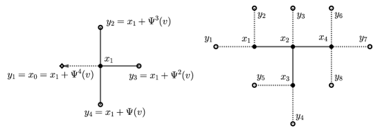
Figure 1. Left: ordering $\prec_{1}$ on $\Delta\{x_{1}\}=\{y_{1},y_{2},y_{3},y_{4}\}$. We have $a(1):=0$, $v=-e_{1}$ and $y_{1}\prec y_{2}\prec y_{3}\prec y_{4}$. Right: ordering on the boundary of $\Delta\{x_{1},x_{2},x_{3},x_{4}\}=\{y_{1},\ldots,y_{8}\}$. We have $y_{1}\prec y_{2}\prec\cdots\prec y_{8}$. A dotted segment is drawn between two points $y_{i}$ and $x_{j}$ if the point $y_{i}$ is a neighbor of $x_{j}$ but not of $x_{j+1},\dots,x_{4}$.

Suppose that we have a procedure to decide, given $\theta\in\Theta$ (cf. Definition 3.2), $x_{1},x_{2},\dots,x_{n},x_{n+1}\in\Lambda$ and $x\in\{x_{1},\dots,x_{n}\}$, if the point $x_{n+1}\in\Lambda$ is occupied (for $n=0$) and if it is occupied and linked to $x$ (for $n\geq 1$), knowing the occupation state of the points $x_{1},x_{2},\dots,x_{n}\in\Lambda$ and the presence or absence of links between them. The precise definition of occupation and link is not relevant now, here we assume that these properties have been previously defined and that can be checked knowing $\theta$.

We now define a random field $\zeta=\left(\zeta(x)\,:\,x\in\Lambda\right)$ with $\zeta(x)\in\{0,1\}$ on the probability space $\bigl{(}\Theta,{\mathbb{Q}}\bigr{)}$. ${\mathbb{Q}}$ is a probability measure on $\Theta$, which can differ from the probability ${\mathbb{P}}$ appearing in Definition 3.2 (in the application ${\mathbb{Q}}$ will be a suitable conditioning of ${\mathbb{P}}$). To define the field $\zeta$, we build below the sets $C^{s}_{j}=(E^{s}_{j},F^{s}_{j})$, with $s\in\{0,1,\dots,M-1\}$ and $j=1,2,\dots,M^{2}$. The construction will fulfill the following properties:

• $E^{s}_{j}$ will be a connected subset of $\Lambda$;

• there exists $J^{s}\in\{1,2\dots,M^{2}\}$ such that, for $j<J^{s}$, $C^{s}_{j+1}=(E^{s}_{j+1},F^{s}_{j+1})$ will be obtained from $C^{s}_{j}=(E^{s}_{j},F^{s}_{j})$ by adding exactly a point (called $x^{s}_{j+1}$) either to $E^{s}_{j}$ or to $F^{s}_{j}$; while, for $j\geq J^{s}$, $C^{s}_{j+1}=(E^{s}_{j+1},F^{s}_{j+1})$ will equal $C_{j}^{s}=(E^{s}_{j},F^{s}_{j})$;

• $\zeta\equiv 1$ on $E^{s}_{j}$ and $\zeta\equiv 0$ on $F^{s}_{j}$.

Note that, because of the above rules, $E^{s}_{j}\cup F^{s}_{j}=\{x^{s}_{1},x^{s}_{2},\dots,x^{s}_{j}\}$ for $1\leq j\leq J^{s}$. In order to make the construction clearer, in Appendix A we illustrate the construction in a particular example.

We now start with the definitions involved in the construction. In what follows, the index $s$ will vary in $\{0,1,\dots,M-1\}$. We also set $x^{s}_{1}:=(0,s)$. We build the sets $C^{0}_{1}$, $C^{1}_{1}$,…,$C^{M-1}_{1}$ as follows. If the point $x^{s}_{1}$ is occupied, then we set

$$\zeta(x^{s}_{1}):=1\text{ and }C^{s}_{1}:=\left(E^{s}_{1},F^{s}_{1}\right):=(\{x^{s}_{1}\},\emptyset)\,,$$ (31)

otherwise we set

$$\zeta(x^{s}_{1}):=0\text{ and }C^{s}_{1}:=\left(E^{s}_{1},F^{s}_{1}\right):=(\emptyset,\{x^{s}_{1}\})\,.$$ (32)

We then define iteratively

$$C^{0}_{2},\;C^{0}_{3},\dots,\;C^{0}_{M^{2}},\;C^{1}_{2},\;C^{1}_{3},\dots,\;C^{1}_{M^{2}},\dots,\;C^{M-1}_{2},\;C^{M-1}_{3},\dots,\;C^{M-1}_{M^{2}}$$ (33)

as follows. If $E^{s}_{1}=\emptyset$, then we declare $J^{s}:=1$, thus implying that $C_{1}^{s}=C_{2}^{s}=\cdots=C_{M^{2}}^{s}$. We restrict now to the case $E^{s}_{1}\not=\emptyset$. Suppose that we have defined all the sets preceding $C^{s}_{j+1}$ in the above string (33) (i.e. up to $C^{s}_{j}$), that we have not declared that $J^{s}$ equals some value in $\{1,2,\dots,j\}$ and that we want to define $C^{s}_{j+1}$. We call $W^{s}_{j}$ the points of $\Lambda$ involved in the construction up to this moment, i.e.

$$W^{s}_{j}=\{x_{1}^{k}:0\leq k\leq M-1\}\cup\{x^{s^{\prime}}_{r}:0\leq s^{\prime}<s,\,1<r\leq M^{2}\}\cup\{x^{s}_{r}:1<r\leq j\}\,.$$

As already mentioned, it must be $E^{s}_{0}\subset E^{s}_{1}\subset\cdots\subset E^{s}_{j}$ and at each inclusion either the two sets are equal or the second one is obtained from the first one by adding exactly a point. We then write $\bar{E}^{s}_{j}$ for the non–empty string obtained as follows: the entries of $\bar{E}^{s}_{j}$ are the elements of $E^{s}_{j}$, moreover if $x^{s}_{a},x^{s}_{b}\in E^{s}_{j}$ and $a<b$, then $x^{s}_{a}$ appears in $\bar{E}^{s}_{j}$ before $x^{s}_{b}$. Note that the above property “$x^{s}_{a},x^{s}_{b}\in E^{s}_{j}$ and $a<b$” simply means that the point $x^{s}_{a}$ has been added before $x^{s}_{b}$ to one of the sets $E^{s}_{0}\subset E^{s}_{1}\subset\cdots\subset E^{s}_{j}$. Then, on $\Delta E^{s}_{j}$ we have the ordering $\prec$ (initially defined) associated to the string $\bar{E}^{s}_{j}$. We call $\mathcal{P}^{s}_{j}$ the following property: $E^{s}_{j}$ is disjoint from the right vertical face of $\Lambda$, i.e. $E^{s}_{j}\cap\left(\{M+1\}\times\{0,1,\dots,M-1\}\right)=\emptyset$, and $(\Lambda\cap{\color[rgb]{0,0,0}\Delta{E}^{s}_{j}})\setminus W^{s}_{j}\not=\emptyset$. If property $\mathcal{P}^{s}_{j}$ is satisfied, then we denote by $x^{s}_{j+1}$ the last element of $(\Lambda\cap{\color[rgb]{0,0,0}\Delta{E}^{s}_{j}})\setminus W^{s}_{j}$ w.r.t. $\prec$. We define $k$ as the largest integer $k$ such that $x_{k}^{s}\in E^{s}_{j}$ and $|x^{s}_{j+1}-x^{s}_{k}|=1$. If $x^{s}_{j+1}$ is occupied and linked to $x^{s}_{k}$, then we set

$$\zeta(x^{s}_{j+1}):=1\text{ and }C^{s}_{j+1}:=\left(E^{s}_{j}\cup\{x^{s}_{j+1}\},F^{s}_{j}\right)\,,$$ (34)

otherwise we set

$$\zeta(x^{s}_{j+1}):=0\text{ and }C^{s}_{j+1}:=\left(E^{s}_{j},F^{s}_{j}\cup\{x^{s}_{j+1}\}\right)\,.$$ (35)

On the other hand, if property $\mathcal{P}^{s}_{j}$ is not verified, then we declare $J^{s}:=j$, thus implying that $C_{j}^{s}=C_{j+1}^{s}=\cdots=C_{M^{2}}^{s}$.

It is possible that the set $\cup_{s=0}^{M-1}\cup_{j=1}^{M^{2}}\left(E^{s}_{j}\cup F^{s}_{j}\right)$ does not fill all $\Lambda$. In this case we set $\zeta\equiv 0$ on the remaining points. This completes the definition of the random field $\zeta$.

Above we have constructed the sets $C^{s}_{j}$ in the following order: $C^{0}_{1}$, $C^{1}_{1}$, $\dots$, $C^{M-1}_{1}$, $C^{0}_{2}$, $C^{0}_{3}$, $\dots,$ $C^{0}_{M^{2}},$ $C^{1}_{2},$ $C^{1}_{3},$ $\dots,$ $C^{1}_{M^{2}},$ $\dots,$ $C^{M-1}_{2},$ $C^{M-1}_{3},$ $\dots,$ $C^{M-1}_{M^{2}}$.

We make the following assumption:

Assumption (A): For some $p\in[0,1]$ at every step in the above construction the probability to add a point to a set of the form $E^{s}_{j}$, conditioned to the construction performed before such a step, is lower bounded by $p$.

Call $N_{M}$ the maximal number of vertex-disjoint LR crossings of the box $\Lambda$ for $\zeta$, where $\{x,y\}$ is an edge if $x$ and $y$ are distinct, linked, occupied sites. Here crossings are the standard ones for percolation on ${\mathbb{Z}}^{2}$ [11]. Note that $N_{M}$ also equals the number of indexes $s\in\{0,1,\dots,M-1\}$ such that $E^{s}_{M^{2}}$ intersects the right vertical face of $\Lambda$. By establishing a stochastic domination on a 2–dimensional site percolation in the same spirit of [12, Lemma 1] (cf. [18, Lemma 4.1]), due to Assumption (A) the following holds:

Lemma 4.1.

Under Assumption (A) $N_{M}$ stochastically dominates the maximal number of vertex-disjoint LR crossings in $\Lambda$ for a site percolation on ${\mathbb{Z}}^{2}$ of parameter $p$.

Due to the above lemma and the results on LR crossings for the Bernoulli site percolation (cf. [12, Remark (d)]), we get:

Corollary 4.2.

If Assumption (A) is fulfilled with $p>p_{c}(2)$, where $p_{c}(2)$ is the critical probability for the site percolation on ${\mathbb{Z}}^{2}$, then there exist constants $c,c^{\prime}>0$ such that ${\mathbb{Q}}(N_{M}\geq cM)\geq 1-e^{-c^{\prime}M}$ for any positive integer $M$.

5. Proof of Eq. (25) as a byproduct of Tanemura’s algorithm and renormalization

In this section we prove Eq. (25) by combining Tanemura’s algorithm and a renormalization scheme inspired by the one in [12]. For the latter we will not discuss here all technical aspects, and postpone a detailed treatment to the next sections.

Given $m\in{\mathbb{N}}_{+}$ and $z\in\varepsilon{\mathbb{Z}}^{d}$ we set

$$B(m):=[-m,m]^{d}\cap\varepsilon{\mathbb{Z}}^{d}\text{ and }B(z,m):=z+B(m)\,.$$ (36)

Recall that $U_{*}:=U_{*}(\alpha/2)$ (cf. Assumption (A4) and Definition 3.1) and that $\Delta={\rm supp}(\nu)$ and $\sup h=1$ (cf. Warning 3.1). Note also that, since the structural function $h$ is symmetric, by applying twice (5) we get $h(a,\tilde{a})\geq h(b,\tilde{a})-\alpha/2\geq h(b,\tilde{b})-\alpha$ for any $b,\tilde{b}\in\Delta$ and $a,\tilde{a}\in U_{*}$. Hence, we have

$$h(a,\tilde{a})\geq\sup_{b,\tilde{b}\in\Delta}h(b,\tilde{b})-\alpha=1-\alpha\qquad\forall a,\tilde{a}\in U_{*}\,.$$ (37)

Definition 5.1 (Seed).

Given $z\in\varepsilon{\mathbb{Z}}^{d}$ and $m\in{\mathbb{N}}_{+}$, we say that $B(z,m)$ is a seed if $A_{x}\in U_{*}$ for all $x\in B(z,m)$.

Recall the graph ${\mathbb{G}}_{-}=({\mathbb{V}}_{-},{\mathbb{E}}_{-})$ introduced in Definition 3.7. Note that any seed is a subset of ${\mathbb{V}}_{-}$. Moreover, a seed is a region of “high connectivity” in the minimal graph ${\mathbb{G}}_{-}$:

Lemma 5.2.

If $B(z,m)$ is a seed, then $B(z,m)$ is a connected subset in the graph ${\mathbb{G}}_{-}$.

Proof.

It is enough to show that $|x-y|\leq h(A_{x},A_{y})-3\alpha$ for any $x,y\in B(z,m)$ with $|x-y|=\varepsilon$. Since $\varepsilon=\alpha/100\sqrt{d}$, we get $|x-y|\leq\alpha/100$. On the other hand, by (37) and since $A_{x},A_{y}\in U_{*}$, we have $h(A_{x},A_{y})\geq 1-\alpha$. To conclude it is enough to recall that $10\alpha\leq 1$ (cf. Definition 3.1). ∎

Recall that $p_{c}(2)$ is the critical probability for site percolation on ${\mathbb{Z}}^{2}$. We now fix some relevant constants and recall the definitions of others:

• We fix $\varepsilon^{\prime}\in(0,1)$ such that $1-6\varepsilon^{\prime}\geq 3/4>p_{c}(2)$.

• We fix positive integers $m\leq n$ satisfying the properties stated in Lemma 6.4 in Section 6 (their precise value is not relevant to follow the arguments below).

• Recall Definition 3.1 for $\varepsilon$.

• We let $N:=n+m+\varepsilon$.

• $L$ is a positive number as in (25).

• Given $L$, the constant $M$ (introduced in (30)) is defined as the smallest positive integer such that $4N(M+1)>2L+5+m+N$ (in particular, $M$ and $L$ are of the same order).

In the rest of this section we explain how to get (25) with $k=4N$. As we will see in a while, such a choice of $k$ guarantees independence properties in the construction of left-right crossings.

As in Tanemura’s algorithm we take $\Lambda:=([0,M+1]\times[0,M-1])\cap{\mathbb{Z}}^{2}$ (in general we will use the notation introduced in Section 4). We recall that $x_{1}^{s}:=(s,0)$ for $s=0,1,\dots,M-1$. We set

$$\bar{x}:=(x,0,0,\dots,0)\in{\mathbb{Z}}^{d}\text{ for }x\in{\mathbb{Z}}^{2}\,.$$ (38)

Below, we will naturally associate to each point $x\in\Lambda$ the point $4N\bar{x}$ in the renormalized lattice $4N{\mathbb{Z}}^{d}\subset\varepsilon{\mathbb{Z}}^{d}$.

Definition 5.3 (Conditional probability ${\mathbb{Q}}$).

We set ${\mathbb{Q}}(\cdot):={\mathbb{P}}(\cdot\,|\,D)$ where

$$D:=\{B(4N\bar{x}_{1}^{s},m)\text{ is a seed }\forall x_{1}^{s}\in\Lambda\}$$ (39)

To run Tanemura’s algorithm we first need to define when the point $x_{1}^{s}$ is occupied. Our definition will imply that the graph ${\mathbb{G}}\subset{\mathbb{G}}_{+}$ contains a cluster centered at $4N\bar{x}_{1}^{s}$ as in Fig. 2 (left), when $d=2$. In particular, the seed $B(4N\bar{x}_{1}^{s},m)$ is connected in ${\mathbb{G}}_{+}$ by a cluster of points lying inside the box $B(4N\bar{x}_{1}^{s},n)$ to four seeds adjacent to the faces of such a box in the directions $\pm e_{1}$, $\pm e_{2}$ ($e_{1},e_{2},\dots,e_{d}$ being the canonical basis of ${\mathbb{R}}^{d}$). The precise definition (for all $d\geq 2$) of the occupation of $x_{1}^{s}$ is rather technical and explained in Section 7 (it corresponds to Definition 7.2, when $\bar{x}_{1}^{s}$ is thought of as the new origin of $\varepsilon{\mathbb{Z}}^{d}$). We point out that the cluster appearing in Fig. 2 (left) is contained in a box of radius $N+m<2N$ centered at at $4N\bar{x}^{s}_{1}$. So, to verify that $\bar{x}_{1}^{s}$ is occupied, it is enough to know the random variables $A_{z}$ with $z$ in the interior of the box $B(4N\bar{x}^{s}_{1},2N)$. Since the above interior parts are disjoint when varying $s$, we conclude that the events $\{x_{1}^{s}\text{ is occupied}\}$ are ${\mathbb{Q}}$–independent when varying $s$ among $\{0,1,\dots,M-1\}$. Moreover, by Proposition 7.4, ${\mathbb{Q}}(x_{1}^{s}\text{ is occupied})\geq 1-4\varepsilon^{\prime}$.

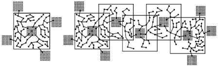
Figure 2. Left: cluster contained in ${\mathbb{G}}_{+}$ when $x_{1}^{s}$ is occupied for $d=2$, the centered grey circle corresponds to $4N\bar{x}_{1}^{s}$, the large box has radius $n$, the smaller boxes have radius $m$ and are seeds. Right: cluster of ${\mathbb{G}}_{+}$ related to the definition of $(0,0)\to(1,0)$ knowing that $x^{0}_{1}=(0,0)$ is occupied, the two grey circles are given by $0$ and $4Ne_{1}$.

Knowing the occupation state of $x_{1}^{s}$, we can define the sets $C_{1}^{0},C_{1}^{1},\dots,C_{1}^{M-1}$ in Tanemura’s algorithm. Let us move to $C^{0}_{2}$. Let us assume for example that $x_{1}^{0}=(0,0)$ is occupied, hence $C^{1}_{0}=(\{x^{0}_{1}\},\emptyset)$. Then, by Tanemura’s algorithm, one should check if $(1,0)$ is occupied and linked to the origin $x_{1}^{0}$ or not. We have first to define this concept. To this aim we need to explore the graph ${\mathbb{G}}_{+}$ in the direction $e_{1}$ from the origin. Roughly, when $d=2$, we say that $(1,0)$ is linked to $(0,0)$ and occupied (shortly, $(0,0)\to(0,1)$) if the graph ${\mathbb{G}}_{+}$ contains a cluster similar to the one in Fig. 2 (right) and Fig. 3, extending the cluster appearing in Fig. 2 (left). Note that there is a seed (called $s_{5}$ in Fig. 3) in the proximity of $4Ne_{1}$ (the grey circle on the right in Fig. 2 (right) and Fig. 3) connected to four seeds neighboring the box of radius $n$ concentric to $s_{5}$, one for each face in the directions $\pm e_{1},\pm e_{2}$. Hence, we have a local geometry similar to the one of Fig. 2 (left). Moreover, see Fig. 3, the cluster turns in direction $e_{1}$ and connects inside ${\mathbb{G}}_{+}$ the seed $s_{1}$ at $4N\bar{x}^{1}_{0}=0$ to the seed $s_{5}$ around $4Ne_{1}$ by passing through the intermediate seeds $s_{2},s_{3},s_{4}$. Note that, in order to assure that $s_{5}$ lays around $4Ne_{1}$ the intermediate seeds have to be located alternatively up and down. The precise definition (for all $d\geq 2$) of the event $\{(0,0)\to(1,0)\}$, knowing that $x_{1}^{0}=(0,0)$ is occupied, is given by Definition 7.11 in Section 7. Having defined this concept, we can build the set $C^{0}_{2}$ in Tanemura’s algorithm.

We move to $C^{0}_{3}$. Suppose for example that $(0,0)\to(1,0)$ occurs, hence $C^{0}_{2}=\bigl{(}\{(0,0),(1,0)\},\emptyset\bigr{)}$. Then, according to Tanemura’s algorithm, we need to check if $(2,0)$ is linked to $(1,0)$ and occupied (shortly, $(1,0)\to(2,0)$). The definition of the last event is similar to the one of “$(0,0)\to(1,0)$”. Roughly, by means of three intermediate seeds (the first one given by $s_{6}$ in Fig. 3) there is a cluster in ${\mathbb{G}}_{+}$ similar to the one in Fig. 2 (right) connecting the seed in the proximity of $4Ne_{1}$ to a seed in the proximity $8Ne_{1}$ and this last seed is connected to four seeds adjacent to the faces in the directions $\pm e_{1},\pm e_{2}$ of a concentric box of radius $n$. Let us suppose for example that $(1,0)\not\to(2,0)$. Then $C^{0}_{3}=\bigl{(}\{(0,0),(1,0)\},\{(2,0)\}\bigr{)}$.

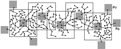
Figure 3. Same cluster as in Figure 2 (right). $s_{1},s_{2},\dots,s_{7}$ are seeds used to progressively extend the cluster along the construction.

We move to $C^{0}_{4}$. According to Tanemura’s algorithm, we need to check if $(1,0)$ is linked to $(1,1)$ and occupied, shortly $(1,0)\to(1,1)$. This last concept is roughly defined as follows: by means of three intermediate seeds (the first one given by $s_{7}$ in Fig. 3) there is a cluster in ${\mathbb{G}}_{+}$ connecting the seed $s_{5}$ in the proximity of $4Ne_{1}$ to a seed in the proximity $4Ne_{1}+4Ne_{2}$ and this last seed is connected to four seeds adjacent to the faces in the directions $\pm e_{1},\pm e_{2}$ of a concentric box of radius $n$ (see Fig. 4). We can then build the set $C^{0}_{4}$.

In general, for any $d\geq 2$ and $v\in\{\pm(1,0)\,,\,\pm(0,1)\}$, the precise definition of “$(a,b)\to(a,b)+v$ knowing that $(a,b)$ is occupied” is given by Definition 7.11 apart from changing origin and direction. We point out that in Definition 7.11, and in general in Section 7, we work with ${\mathbb{Z}}^{2}\times\{0\}\subset{\mathbb{Z}}^{d}$ instead of ${\mathbb{Z}}^{2}$ (${\mathbb{Z}}^{2}\times\{0\}$ and ${\mathbb{Z}}^{2}$ are naturally identified).

Proceeding in this way one defines the whole sequence $C^{0}_{2},\;C^{0}_{3},\dots,\;C^{0}_{M^{2}}$. Then one has to build the sequence $C^{1}_{2},\;C^{1}_{3},\dots,\;C^{1}_{M^{2}}$. If $x_{1}^{1}=(0,1)$ is not occupied, i.e. $C^{1}_{1}=(\emptyset,\{(0,1)\})$, then one sets $C^{1}_{1}=C^{1}_{2}=C^{1}_{3}\dots=C^{1}_{M^{2}}$. Otherwise one starts to build a cluster in ${\mathbb{G}}_{+}$ similarly to what done above, with the only difference that $x_{1}^{1}$ replaces $x_{1}^{0}$. As the reader can check, after reading the detailed definitions in Section 7, the region of $\varepsilon{\mathbb{Z}}^{d}$ explored when checking linkages and occupations for the cluster blooming from $x_{1}^{1}$ is far enough from the region explored for the cluster blooming from $x_{1}^{0}$, and no spatial correlation emerges. One proceeds in this way to complete Tanemura’s algorithm.

In Section 7 we will analyze in detail the basic steps of the above construction and show (see the discussion in Section 7.5) the validity of Assumption (A) of Section 4 with $p=1-6\varepsilon^{\prime}>p_{c}(2)$. As a consequence we can apply Corollary 4.2 and get that there exist constants $c_{1},c_{2}>0$ such that ${\mathbb{Q}}(N_{M}\geq c_{1}M)\geq 1-e^{-c_{2}M}$, where $N_{M}$ is the maximal number of vertex-disjoint LR crossings of $\Lambda$ for the graph with vertexes given by occupied sites and having edges between nearest–neighbor linked occupied sites.

As rather intuitive and detailed in Appendix C, there is a constant $C>0$ (independent from $M$) such that that event $\{N_{M}\geq c_{1}M\}$ implies that the graph ${\mathbb{G}}_{+}$ has at least $CM$ vertex-disjoint LR crossings of a 2d slice of size $O(L)\times O(L)\times O(N)^{d-2}$ (recall that $L\asymp M$). In particular, as discussed in Appendix C, the bound ${\mathbb{Q}}(N_{M}\geq c_{1}M)\geq 1-e^{-c_{2}M}$ implies the estimate (25) with $k=4N$ and new positive constants $c_{1},c_{2}$ there.

Figure 4. Further extension of the cluster in ${\mathbb{G}}_{+}$ when $(1,0)\to(1,1)$.

6. Renormalization: preliminary tools

In the rest we will often write ${\mathbb{P}}(E_{1},E_{2},\dots,E_{n})$ instead of ${\mathbb{P}}(E_{1}\cap E_{2}\cap\cdots\cap E_{n})$, also for other probability measures. For the readers convenience we recall Definitions 3.3 and 3.7 of the graphs ${\mathbb{G}}_{+}=({\mathbb{V}}_{+},{\mathbb{E}}_{+})$ and ${\mathbb{G}}_{-}=({\mathbb{V}}_{-},{\mathbb{E}}_{-})$:

$${\mathbb{V}}_{-} :=\{z\in\varepsilon{\mathbb{Z}}^{d}\,:\,A_{z}\in{\mathbb{R}}\}\,,$$

$${\mathbb{E}}_{-} :=\left\{\{z,z^{\prime}\}:z\not=z^{\prime}\text{ in }{\mathbb{V}}_{-}\,,\;|z-z^{\prime}|\leq h(A_{z},A_{z^{\prime}})-3\alpha\right\}\,,$$

$${\mathbb{V}}_{+} :=\{z\in\varepsilon{\mathbb{Z}}^{d}\,:\,A^{\rm au}_{z}\in{\mathbb{R}}\}\,,$$

$${\mathbb{E}}_{+} :=\left\{\{z,z^{\prime}\}:z\not=z^{\prime}\text{ in }{\mathbb{V}}\,,\;\;\;|z-z^{\prime}|\leq h(A^{\rm au}_{z},A^{\rm au}_{z^{\prime}})-\alpha\right\}\,.$$

We also introduce the intermediate graph ${\mathbb{G}}$ (trivially, we have ${\mathbb{G}}_{-}\subset{\mathbb{G}}\subset{\mathbb{G}}_{+}$):

Definition 6.1 (Graph ${\mathbb{G}}=({\mathbb{V}},{\mathbb{E}})$).

On the probability space $(\Theta,{\mathbb{P}})$ we define the graph ${\mathbb{G}}=({\mathbb{V}},{\mathbb{E}})$ as

$${\mathbb{V}}:=\{z\in\varepsilon{\mathbb{Z}}^{d}\,:\,A_{z}\in{\mathbb{R}}\}\,,$$ (40)

$${\mathbb{E}}:=\left\{\{z,z^{\prime}\}:z\not=z^{\prime}\text{ in }{\mathbb{V}}_{-}\,,\;|z-z^{\prime}|\leq h(A_{z},A_{z^{\prime}})-2\alpha\right\}\,\,.$$ (41)

We introduce the following conventions:

• Given $x\in{\mathbb{V}}$ and $C\subset{\mathbb{V}}$ with $x\not\in C$, we say that $x$ is adjacent to $C$ inside ${\mathbb{G}}$ if there exists $y\in C$ such that $\{x,y\}\in{\mathbb{E}}$.

• Given $A,B,C\subset\varepsilon{\mathbb{Z}}^{d}$, we say that “$A\leftrightarrow B$ in $C$ for ${\mathbb{G}}$” if there exist $x_{1},x_{2},\dots,x_{k}\in C\cap{\mathbb{V}}$ such that $x_{1}\in A$, $x_{k}\in B$ and $\{x_{i},x_{i+1}\}\in{\mathbb{E}}$ for all $i:1\leq i<k$.

• Given a bounded set $A\subset{\mathbb{R}}^{d}$ we say that “$A\leftrightarrow\infty$ for ${\mathbb{G}}$” if there exists an unbounded path in ${\mathbb{G}}$ starting at some point in $A$.

Similar definitions hold for the graphs ${\mathbb{G}}_{-}=({\mathbb{V}}_{-},{\mathbb{E}}_{-})$ and ${\mathbb{G}}_{+}=({\mathbb{V}}_{+},{\mathbb{E}}_{+})$.

Definition 6.2 (Sets $B(m)$, $T(n)$, $T(m,n)$, $K(m,n)$).

For $m\leq n\in{\mathbb{N}}_{+}$ we define the following sets:

$$B(m):=[-m,m]^{d}\cap\varepsilon{\mathbb{Z}}^{d}\text{ and }B(z,m):=z+B(m)\,,$$

$$T(n):=\{x\in\varepsilon{\mathbb{Z}}^{d}:n-1<\|x\|_{\infty}\leq n,\,0\leq x_{i}\leq x_{1}\;\forall i=1,2,\dots,d\}\,,$$

$$T(m,n):=\bigl{(}[n+\varepsilon,n+\varepsilon+2m]\times[0,n]^{d-1}\bigr{)}\cap\varepsilon{\mathbb{Z}}^{d}\,,$$

$${\color[rgb]{0,0,0}K(m,n):=\{x\in{\mathbb{V}}\cap T(n):\text{$x$ is adjacent in ${\mathbb{G}}$ to a seed included in $T(m,n)$}\}\,.}$$

For the reader’s convenience, in the above definition we have also recalled (36). We refer to Figure 5-(left) for some illustration. We recall that seeds have been introduced in Definition 5.1. The definition of $K(m,n)$ can be restated as follows: $K(m,n)$ is given by the points $x\in{\mathbb{V}}\cap T(n)$ such that, for some $z\in\varepsilon{\mathbb{Z}}^{d}$, the box $B(z,m)\subset T(m,n)$ is a seed and $\exists y\in B(z,m)$ with $\{x,y\}\in{\mathbb{E}}$.

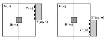
Figure 5. Left: sets $T(n)$ and $T(m,n)$. Right: sets $T^{*}(n)$ and $T^{*}(m,n)$.

The following proposition is the analogous of [12, Lemma 5] in our context. It will enter in the proof of Lemma 6.4 and in the proof of Proposition 7.4 (which lower bounds from below the probability that in the first step of the renormalization scheme we enlarge the cluster of occupied sites).

Proposition 6.3.

Given $\eta\in(0,1)$, there exist positive integers $m=m(\eta)$ and $n=n(\eta)$ such that $m>2$, $2m<n$, $2m|n$ and

$${\mathbb{P}}\bigl{(}B(m)\leftrightarrow K(m,n)\text{ in $B(n)$ for }{\mathbb{G}}\bigr{)}>1-\eta\,.$$ (42)

This proposition is a consequence of Lemma 3.8 concerning the percolation of graph ${\mathbb{G}}_{-}$. Even if having a seed in a specific place is an event of small probability, the big number of possible configurations for the seed entering in the definition of $K(m,n)$ makes the event in (42) of high probability. We postpone the proof of Proposition 6.3 to Section 9.

It is convenient to introduce the function $h_{*}:\Delta\to{\mathbb{R}}$ defined as

$$h_{*}(a):=\sup_{b\in\Delta}h(a,b)\,.$$ (43)

Moreover, given a finite set $R\subset\varepsilon{\mathbb{Z}}^{d}$, we define the non–random boundary set

$$\partial R\,:=\{y\in\varepsilon{\mathbb{Z}}^{d}\setminus R\,:\,d(y,R)\leq 1-2\alpha\}\,,$$ (44)

where $d(\cdot,\cdot)$ denotes the Euclidean distance. Note that the edges of ${\mathbb{G}}$ have length bounded by $1-2\alpha$. To avoid ambiguity, we point out that in what follows the set $\partial R\cap B(n)$ has to be thought of as $(\partial R)\cap B(n)$ and not as $\partial(R\cap B(n))$.

The following lemma (which is the analogous of [12, Lemma 6] in our context) will be crucial in estimating from below the probability to enlarge the occupied cluster at a generic step of the renormalization scheme (cf. Section 5). More specifically, it will allow to prove Proposition 7.12 and to control the further steps in the renomalization scheme as explained in Section 7.5. Recall Definition 3.1 of $U_{*}$.

Lemma 6.4.

Fix $\varepsilon^{\prime}\in(0,1)$. Then there exist positive integers $m$ and $n$, with $m>2$, $2m<n$ and $2m|n$, satisfying the following property.

Consider the following sets (see Figure 6):

• Let $R$ be a finite subset of $\varepsilon{\mathbb{Z}}^{d}$ satisfying

  $$B(m)\subset R\,,\qquad\left(R\cup\partial R\right)\cap\left(T(n)\cup T(m,n)\right)=\emptyset\,.$$ (45)

• For any $x\in R\cup\partial R$, let $\Lambda(x)$ be a subset of $\{1,2,\dots,K\}$. We suppose that there exists $k_{*}\in\{1,2,\dots,K\}$ such that

  $$k_{*}\not\in\cup_{x\in D}\Lambda(x)\,,$$ (46)

  where $D\subset\varepsilon{\mathbb{Z}}^{d}$ is defined as

  $$\begin{split}D:=&\left(\partial R\cap B(n)\right)\\ &\cup\left\{x\in R\,:\,\exists y\in\partial R\cap B(n)\text{ with }|x-y|\leq 1-2\alpha\right\}\,.\end{split}$$ (47)

Consider the following events:

• Let $H$ be any event in the $\sigma$–algebra $\mathcal{F}$ generated by the random variables $(A_{x})_{x\in R\cup\partial R}$ and $(T_{x}^{(j)})_{x\in R\cup\partial R\,,\,j\in\Lambda(x)}$.

• Let $G$ be the event that there exists a string $(z_{0},z_{1},z_{2},\dots,z_{\ell})$ in ${\mathbb{V}}$ such that

  • $z_{0}\in R$;

  • $z_{1}\in\partial R\cap B(n)$;

  • $z_{2},\dots,z_{\ell}\in B(n)\setminus\bigl{(}R\cup\partial R\bigr{)}$;

  • $z_{2},\dots,z_{\ell}$ is a path in ${\mathbb{G}}$;

  • $z_{\ell}\in K(m,n)$;

  • $T^{(k_{*})}_{z_{0}}\in U_{*}$ and $T^{(k_{*})}_{z_{1}}\in U_{*}$;

  • $|z_{0}-z_{1}|\leq 1-2\alpha$;

  • $|z_{1}-z_{2}|\leq{\color[rgb]{0,0,0}h_{*}(A_{z_{2}})}-2\alpha$.

Then ${\mathbb{P}}(G\,|\,H)\geq 1-\varepsilon^{\prime}$.

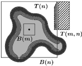
Figure 6. $\partial R$ is the very dark grey contour. $R$ is given by the light/dark grey region around the origin. $D\setminus\bigl{(}\partial R\cap B(n)\bigr{)}$ is the dark grey subset of $R$.

We postpone the proof of Lemma 6.4 to Section 10. We point out that the above properties (P6), (P7), (P8) (which can appear a little exotic now) will be crucial to derive the ${\color[rgb]{0,0,0}{\mathbb{G}}_{+}}$–connectivity issue stated in Lemma 6.7 below. Indeed, although $(z_{0},z_{1},z_{2},\dots,z_{\ell})$ could be not a path in ${\mathbb{G}}$, one can prove that it is a path in ${\color[rgb]{0,0,0}{\mathbb{G}}_{+}}$.

6.1. The sets $E\bigl{[}C,B,i\bigr{]}$ and $F\bigl{[}C,B,B^{\prime},i\bigr{]}$

In the next section we will iteratively construct random subsets of $\varepsilon{\mathbb{Z}}^{d}$ sharing the property to be connected in ${\mathbb{G}}_{+}$. We introduce here the fundamental building blocks, which are given by the sets $E\bigl{[}C,B,i\bigr{]}$ and $F\bigl{[}C,B,B^{\prime},i\bigr{]}$ (they will appear again in Definition 7.6):

Definition 6.5 (Sets $E\bigl{[}C,B,i\bigr{]}$ and $F\bigl{[}C,B,B^{\prime},i\bigr{]}$).

Given three sets $C,B,B^{\prime}\subset\varepsilon{\mathbb{Z}}^{d}$ and given $i\in\{1,2,\dots,K\}$, we define the random subsets $E,F\subset\varepsilon{\mathbb{Z}}^{d}$ as follows:

• $E$ is given by the points $z_{1}$ in $B\cap\partial C$ such that $T_{z_{1}}^{(i)}{\color[rgb]{0,0,0}\in U_{*}}$ and there exists $z_{0}\in C$ with $|z_{0}-z_{1}|\leq 1-2\alpha$ and $T_{z_{0}}^{(i)}{\color[rgb]{0,0,0}\in U_{*}}$;

• $F$ is given by the points $z\in B^{\prime}$ such that there exists a path $(z_{2},\dots,z_{k})$ inside ${\mathbb{G}}$ where $z_{k}=z$, all points $z_{2},\cdots,z_{k}$ are in $B^{\prime}\setminus(C\cup\partial C)$ and $|z_{1}-z_{2}|\leq h_{*}(A_{z_{2}})-2\alpha$ for some $z_{1}\in E$.

To stress the dependence from $C,B,B^{\prime},i$, we will also write $E\bigl{[}C,B,i\bigr{]}$ and $F\bigl{[}C,B,B^{\prime},i\bigr{]}$.

The proof of the next two lemmas is given in Section 11.

Lemma 6.6.

Let $E=E\bigl{[}C,B,i\bigr{]}$ and $F=F\bigl{[}C,B,B^{\prime},i\bigr{]}$ be as in Definition 6.5. Let $\hat{E},\hat{F}\subset\varepsilon{\mathbb{Z}}^{d}$.

• If the event $\{E=\hat{E}\}\cap\{F=\hat{F}\}$ occurs, then $\hat{E},\hat{F}$ satisfy

  $$\hat{E}\cap\hat{F}=\emptyset\,,\qquad\hat{E}\subset\bigl{(}B\cap\partial C\bigr{)}\,,\qquad\hat{F}\subset B^{\prime}\setminus(C\cup\partial C)\,.$$ (48)

• If $\hat{E},\hat{F}$ satisfy (48), then the event $\{E=\hat{E}\}\cap\{F=\hat{F}\}$ belongs to the $\sigma$–algebra generated by

  • $T^{(i)}_{z}$ with $z\in\bigl{(}B\cap\partial C\bigr{)}\cup D$, where

    $$D:=\left\{x\in C\,:\,\exists y\in B\cap\partial C\text{ with }|x-y|\leq 1-2\alpha\right\}\,;$$

  • $A_{z}$ with $z$ belonging to some of the following sets:

    $$\hat{F}\,,\quad\bigl{(}B^{\prime}\setminus(C\cup\partial C)\bigr{)}\cap\partial\hat{F}\,,\quad\bigl{(}B^{\prime}\setminus(C\cup\partial C)\bigr{)}\cap\partial\hat{E}\,.$$

• As a consequence, given $R\subset\varepsilon{\mathbb{Z}}^{d}$, the event $\{E\cup F=R\}$ belongs to the $\sigma$–algebra generated by $\{T^{(i)}_{z}\,:\,z\in\bigl{(}B\cap\partial C\bigr{)}\cup D\}\cup\{A_{z}\,:\,z\in R\cup\partial R\}$.

Lemma 6.7.

Given sets $C,B,B^{\prime}\subset\varepsilon{\mathbb{Z}}^{d}$ and an index $i\in\{1,2,\dots,K\}$, we define $E:={\color[rgb]{0,0,0}E\bigl{[}C,B,i\bigr{]}}$ and $F:=F\bigl{[}C,B,B^{\prime},i\bigr{]}$. If $C\subset{\color[rgb]{0,0,0}{\mathbb{V}}_{+}}$ is connected in the graph ${\color[rgb]{0,0,0}{\mathbb{G}}_{+}=({\mathbb{V}}_{+},{\mathbb{E}}_{+})}$, then the set $C^{\prime}:=C\cup E\cup F$ is contained in ${\color[rgb]{0,0,0}{\mathbb{V}}_{+}}$ and is connected in the graph ${\color[rgb]{0,0,0}{\mathbb{G}}_{+}}$.

7. Renormalization scheme

As in Section 5, we set $N:=n+m+\varepsilon$. From now on $\varepsilon^{\prime}$ is a fixed constant in $(0,1)$ such that $1-6\varepsilon^{\prime}\geq 3/4>p_{c}(2)$, $p_{c}(2)$ being the critical probability for Bernoulli site percolation on ${\mathbb{Z}}^{2}$. Moreover, we choose $m,n$ as in Lemma 6.4.

Recall Definition 6.2 of $T(n)$, $T(m,n)$. We define

$$T^{*}(m,n):=f\left(T(m,n)\right)\text{ and }T^{*}(n):=f\left(T(n)\right)\,,$$ (49)

where $f:{\mathbb{R}}^{d}\to{\mathbb{R}}^{d}$ is the isometry $f(x_{1},x_{2},\dots,x_{d}):=(x_{1},-x_{2},\dots,-x_{d})$ (see Figure 5). Given $a\in{\mathbb{R}}^{d}$, we define $g(\cdot|a):{\mathbb{R}}^{d}\to{\mathbb{R}}^{d}$ as the isometry

$$g(x|a):=(x_{1},-\text{sgn}(a_{2})x_{2},\dots,-\text{sgn}(a_{d})x_{d})\,,$$ (50)

where $\text{sgn}(\cdot)$ is the sign function, with the convention that $\text{sgn}(0)=+1$. Note that $f(x)=g(x|0)$.

Let $e_{1},e_{2},\dots,e_{d}$ be the canonical basis of ${\mathbb{R}}^{d}$. We denote by $L_{1},L_{2},L_{3},L_{4}$ the isometries of ${\mathbb{R}}^{d}$ given respectively by $\mathds{1},\theta,\theta^{2},\theta^{3}$, where $\mathds{1}$ is the identity and $\theta$ is the unique rotation such that $\theta(e_{1})=e_{2}$, $\theta(e_{2})=-e_{1}$, $\theta(e_{i})=e_{i}$ for all $i=3,\dots,d$. We define $B_{0}^{\prime}\subset\varepsilon{\mathbb{Z}}^{d}$ as

$$B_{0}^{\prime}:=B(n)\cup\left(\cup_{j=1}^{4}L_{j}\bigl{(}T(m,n)\bigr{)}\right)\,.$$ (51)

Hence, for $d=2$, $B_{0}^{\prime}$ is the region of $\varepsilon{\mathbb{Z}}^{d}$ given by the largest square and the four peripheral rectangles in Figure 7–(left). For $j=1,2,3,4$ we call $K^{(j)}(m,n)$ the random set of points defined similarly to $K(m,n)$ (cf. Definition 6.2) but with $T(m,n)$ and $T(n)$ replaced by $L_{j}\bigl{(}T(m,n)\bigr{)}$ and $L_{j}\bigl{(}T(n)\bigr{)}$, respectively.

Definition 7.1 (Set $C_{1}$ and success-events $S_{0}$, $S_{1}$).

We define $C_{1}$ as the set of points $x\in B_{0}^{\prime}$ such that

$$\{x\}\leftrightarrow B(m)\text{ in $B_{0}^{\prime}$ for }{\mathbb{G}}\,.$$

Furthermore, we define the success-events $S_{0}$ and $S_{1}$ as

$$S_{0}:=\{\,\text{$B(m)$ is a seed}\,\}\,,$$

$$S_{1}:=\{\,\text{$C_{1}$ contains a point of $K^{(j)}(m,n)$ for each $j=1,2,3,4$}\,\}\,.$$

Definition 7.2 (Occupation of the origin).

We say that the origin $0\in{\color[rgb]{0,0,0}\varepsilon{\mathbb{Z}}^{d}}$ is occupied if the event $S_{0}\cap S_{1}$ takes place.

We refer to Figure 7–(left) for an example of the set $C_{1}$ when ${\color[rgb]{0,0,0}S_{0}\cap S_{1}}$ occurs. We note that the event $S_{0}$ implies that $B(m)\subset{\mathbb{V}}$, hence $B(m)\subset C_{1}$.

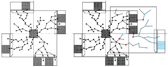
Figure 7. Left: the set $C_{1}$ when $S_{0}\cap S_{1}$ occurs. Right: The set $C_{2}$ when $S_{0}\cap S_{1}\cap S_{2}$ occurs. Points in $C_{1}$ correspond to circles, while points in $C_{2}\setminus C_{1}$ correspond to red rings if in $E_{1}$ and blue triangles if in $F_{1}$.

Remark 7.3.

If the event $S_{0}$ occurs (e.g. if the origin is occupied), then $C_{1}$ is a connected subset of ${\mathbb{G}}$ (and therefore of ${\color[rgb]{0,0,0}{\mathbb{G}}_{+}}$) by Lemma 5.2.

When the origin is occupied, for $i=1,2,3,4$ we define $c^{(i)}$ as the minimal (w.r.t. the lexicographic order) point $z$ in $\varepsilon{\mathbb{Z}}^{d}$ such that $B(z,m)$ is a seed contained in $C_{1}\cap L_{i}\bigl{(}T(m,n)\bigr{)}$. We point out that such a seed exists by Lemma 5.2 and the definition of $S_{1}$. It is simple to check that, when $S_{1}$ takes place,

$${\color[rgb]{0,0,0}c^{(1)}_{1}}=N\text{ and }{\color[rgb]{0,0,0}c^{(1)}_{j}}\in[m,n-m]\text{ for }2\leq j\leq d\,,$$ (52)

where $c^{(1)}_{j}$ denotes the $j$–th coordinate of $c^{(1)}$. Similar formulas hold for $c^{(i)}$, $i=2,3,4$. For later use, we set

$${\color[rgb]{0,0,0}b^{(1)}:=c^{(1)}\,.}$$ (53)

Proposition 7.4.

It holds ${\mathbb{P}}(0\text{ is occupied}\,|\,S_{0})\geq 1-4\varepsilon^{\prime}$.

We postpone the proof of the above proposition to Section 12. If the origin is not occupied, then we stop our construction. Hence, from now on we assume that $0$ is occupied without further mention. We fix a unitary vector, that we take equal to $e_{1}$ without loss of generality, and we explain how we attempt to extend $C_{1}$ in the direction $e_{1}$. In order to shorten the presentation, we will define geometric objects only in the successful cases relevant to continue the construction (in the other cases, the definition can be chosen arbitrarily). Figure 8 will be useful to locate objects.

Below, for $i=2,\dots,7$, we will iteratively define points $b^{(i)}$. Moreover, for $i=1,2,3$, we will iteratively define sets $T_{i}(n)$ and $T_{i}(m,n)$ obtained from $T(n)$ and $T(m,n)$ by an $i$–parametrized orthogonal map. Apart from the case $i=4$, many objects will be defined similarly. Hence, we isolate some special definitions to which we will refer in what follows. We stress that we collect these generic definitions below, but we will apply them only when describing the construction step by step in the next subsections. Recall Definition 6.5.

(i)-Definition 7.5 (Sets $K_{i}(m,n)$, $B_{i}^{\prime}$).

Given $b^{(i)}$, $T_{i}(n)$ and $T_{i}(m,n)$, we define $K_{i}(m,n)$ as the set of points $x\in b^{(i)}+T_{i}(n)$ which are adjacent inside ${\mathbb{G}}$ to a seed contained in $b^{(i)}+T_{i}(m,n)$. Moreover, we define $B_{i}^{\prime}:=b^{(i)}+\bigl{(}B(n)\cup T_{i}(m,n)\bigr{)}$.

(i)-Definition 7.6 (Sets $E_{i},F_{i},C_{i+1}$).

We set

$$E_{i}:={\color[rgb]{0,0,0}E\bigl{[}C_{i},\,B\bigl{(}b^{(i)},n\bigr{)},i]}\,,$$

$$F_{i}:=F\bigl{[}C_{i},\,B\bigl{(}b^{(i)},n\bigr{)},B_{i}^{\prime},i]\,,$$

$$C_{i+1}:=C_{i}\cup E_{i}\cup F_{i}\,.$$

(i)-Definition 7.7 (Success-event $S_{i+1}$).

We call $S_{i+1}$ the success-event that $C_{i+1}$ contains at least one vertex in $K_{i}(m,n)$.

(i)-Definition 7.8 (Property $\mathfrak{p}_{i}$).

We say that property $\mathfrak{p}_{i}$ is satisfied if the sets $C_{i}\cup\partial C_{i}$ and $b^{(i)}+\bigl{(}T_{i}(n)\cup T_{i}(m,n)\bigr{)}$ are disjoint.

In several steps below we will claim without further comments that property $\mathfrak{p}_{i}$ is satisfied. This property will correspond to the second property in (45) in the applications of Lemma 6.4 in Section 12, which (when not immediate) will be checked in Section 12 and Appendixes B.0.1, B.0.2.

Remark 7.9.

If $S_{i+1}$ occurs, then $C_{i+1}$ contains a point $x\in b^{(i)}+T_{i}(n)$ which is adjacent inside ${\mathbb{G}}$ to a seed $B(z,m)$ contained in $b^{(i)}+T_{i}(m,n)\subset B_{i}^{\prime}$. Let us suppose that also property $\mathfrak{p}_{i}$ in Definition 7.8 is satisfied. Then $(C_{i}\cup E_{i})\subset(C_{i}\cup\partial C_{i})$ does not intersect $b^{(i)}+T_{i}(n)$, thus implying that $x\in F_{i}$ ($E_{i}$ and $F_{i}$ were defined in Definition 7.6). Since the above seed $B(z,m)$ is contained in $b^{(i)}+T_{i}(m,n)$, which is contained in $B_{i}^{\prime}\setminus(C_{i}\cup\partial C_{i})$ due to property $\mathfrak{p}_{i}$, by Lemma 5.2 and Definition 6.5 we conclude that $F_{i}\subset C_{i+1}$ contains the above seed $B(z,m)$.

We now continue with the construction of increasing clusters and success-events.

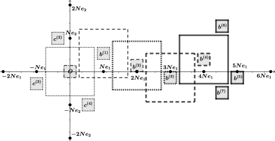
Figure 8. Colored small boxes are the seeds $B(m)$ and $B(b^{(i)},m)$, while bigger boxes are given by $B(n)$ and $B(b^{(i)},n)$.

7.1. Case $i=1$

We define $T_{1}(n):=T^{*}(n)=g\bigl{(}T(n)|b^{(1)}\bigr{)}$ and $T_{1}(m,n)=T^{*}(m,n)=g\bigl{(}T(m,n)|b^{(1)}\bigr{)}$ (cf. (49) and (50)). We apply (i)–Definition 7.5, (i)–Definition 7.6, (i)–Definition 7.7 and (i)–Definition 7.8 for $i=1$. In particular, this defines the sets $K_{1}(m,n),B_{1}^{\prime},E_{1}$, $F_{1}$, $C_{2}$ and the success-event $S_{2}$. See Figure 7–(right).

When $S_{0}\cap S_{1}\cap S_{2}$ occurs, the set $C_{2}$ intersects the box $B(2Ne_{1},N)$ as we now show. Indeed, one can prove property $\mathfrak{p}_{1}$ using (52). Hence, by Remark 7.9, the event $S_{0}\cap S_{1}\cap S_{2}$ implies that $F_{1}\subset C_{2}$ contains a seed inside $b^{(1)}+T^{*}(m,n)$ (see Figure 7–(right)). One can easily check that $b^{(1)}+T^{*}(m,n)\subset B(2Ne_{1},N)$. To this aim we observe that, by (52), if $x\in b^{(1)}+T^{*}(m,n)$, then $x_{1}\in[2N-m,2N+m]\subset 2N+[-N,N]$ and $x_{j}\in[b_{j}^{(1)}-n,b_{j}^{(1)}]\subset[m-n,n-m]\subset[-N,N]$ for $2\leq j\leq d$.

We define $b^{(2)}$ as the minimal point $z\in\varepsilon{\mathbb{Z}}^{d}$ such that $B(z,m)$ is a seed contained in ${\color[rgb]{0,0,0}C_{2}}\cap\bigl{(}b^{(1)}+T^{*}(m,n)\bigr{)}$. By the above discussion, $b^{(1)}+T^{*}(m,n)\subset B(2Ne_{1},N)$. By (52) and since ${\color[rgb]{0,0,0}b^{(2)}_{j}}\in[b^{(1)}_{j}-n,b_{j}^{(1)}]$ for $j\not=1$, we get for $i=2$

$$b^{(i)}_{1}={\color[rgb]{0,0,0}iN},\qquad b^{(i)}_{j}\in[-n+m,n-m]\text{ for }j\not=1\,.$$ (54)

7.2. Case $i=2$

We assume that $S_{0}\cap S_{1}\cap S_{2}$ occurs.

We set ${\color[rgb]{0,0,0}T_{2}}(m,n):=g\left(T(m,n)|{\color[rgb]{0,0,0}b^{(2)}}\right)$ and ${\color[rgb]{0,0,0}T_{2}}(n):=g\left(T(n)|{\color[rgb]{0,0,0}b^{(2)}}\right)$. We apply (i)–Definition 7.5, (i)–Definition 7.6, (i)–Definition 7.7 and (i)–Definition 7.8 for $i=2$. In particular this defines $K_{2}(m,n),B_{2}^{\prime},E_{2},F_{2},C_{3},S_{3}$. It is simple to check that property $\mathfrak{p}_{2}$ is satisfied. If also $S_{3}$ occurs, by Remark 7.9 we can define $b^{(3)}$ as the minimal point in $\varepsilon{\mathbb{Z}}^{d}$ such that $B(z,m)$ is a seed contained in $C_{3}\cap\left(b^{(2)}+T_{2}(m,n)\right)$.

Let us localize some objects. Due to Claim B.1 in Appendix B, $b^{({\color[rgb]{0,0,0}2})}+T_{{\color[rgb]{0,0,0}2}}(m,n)\subset B(3Ne_{1},N)$ (see Figure 8). In particular, if $S_{{\color[rgb]{0,0,0}3}}$ occurs, then $C_{{\color[rgb]{0,0,0}3}}\cap B(3Ne_{1},N)$ contains the above seed $B(z,m)$. If $S_{{\color[rgb]{0,0,0}3}}$ occurs, due to (54) with $i=2$, for $j\not=1$ we have

$$\begin{cases}b_{j}^{({\color[rgb]{0,0,0}3})}\in[b^{({\color[rgb]{0,0,0}2})}_{j}-n+m,b_{j}^{({\color[rgb]{0,0,0}2})}-m]\subset[-n+m,n-2m]&\text{ if $b^{({\color[rgb]{0,0,0}2})}_{j}\geq 0$}\,,\\ b_{j}^{({\color[rgb]{0,0,0}3})}\in[b^{({\color[rgb]{0,0,0}2})}_{j}+m,b_{j}^{({\color[rgb]{0,0,0}2})}+n-m]\subset[-n+2m,n-m],&\text{ if $b^{({\color[rgb]{0,0,0}2})}_{j}<0$}\,.\end{cases}$$ (55)

Due to the above bounds and since $b^{({\color[rgb]{0,0,0}3})}_{1}=3N$, we get that (54) holds also for $i={\color[rgb]{0,0,0}3}$.

7.3. Case ${\color[rgb]{0,0,0}i=3}$

We assume that the event ${\color[rgb]{0,0,0}S_{0}\cap S_{1}\cap S_{2}\cap S_{3}}$ occurs.

We define $T_{{\color[rgb]{0,0,0}3}}(m,n):=g\bigl{(}T(m,n)\,|\,b^{({\color[rgb]{0,0,0}3})}\bigr{)}$ and $T_{{\color[rgb]{0,0,0}3}}(n):=g\bigl{(}T(n)\,|\,b^{({\color[rgb]{0,0,0}3})})$. We apply (i)–Definition 7.5, (i)–Definition 7.6, (i)–Definition 7.7 and (i)–Definition 7.8 for $i={\color[rgb]{0,0,0}3}$. In particular, this defines $K_{3}(m,n),B_{3}^{\prime},E_{3},F_{3},C_{4},S_{4}$. Property $\mathfrak{p}_{3}$ is satisfied. If also $S_{4}$ occurs, by Remark 7.9 we can define $b^{({\color[rgb]{0,0,0}4})}$ as minimal point in $\varepsilon{\mathbb{Z}}^{d}$ such that $B(z,m)$ is a seed in $b^{({\color[rgb]{0,0,0}3})}+T_{{\color[rgb]{0,0,0}3}}(m,n)$.

Let us localize some objects. Due to Claim B.1 in Appendix B, $b^{({\color[rgb]{0,0,0}3})}+T_{{\color[rgb]{0,0,0}3}}(m,n)\subset B(4Ne_{1},N)$ (see Figure 8). In particular, if $S_{4}$ occurs, then ${\color[rgb]{0,0,0}C_{4}}\cap B(4Ne_{1},N)$ contains the above seed $B(z,m)$. When $S_{4}$ occurs, due to (54) for $i=3$ and reasoning as in (55), we get that (54) holds also for $i=4$.

7.4. Case $i=4$

We assume that the event $S_{0}\cap S_{1}\cap\cdots\cap S_{4}$ occurs. The idea now is to connect the cluster $C_{{\color[rgb]{0,0,0}4}}$ to seeds adjacent to the remaining three faces of the cube $b^{({\color[rgb]{0,0,0}4})}+B(n)$ in directions $e_{1}$ and $\pm e_{2}$ (note that we have already the seed $B\bigl{(}b^{(3)},m\bigr{)}$ in the direction $-e_{1}$). To this aim we set

$$\hat{T}_{1}(n):=g\bigl{(}T(n)\,|\,b^{({\color[rgb]{0,0,0}4})}\bigr{)}\qquad\qquad\hat{T}_{1}(m,n):=g\bigl{(}T(m,n)\,|\,b^{({\color[rgb]{0,0,0}4})}\bigr{)}$$

$$\hat{T}_{2}(n):=(h\circ\theta)\bigl{(}\hat{T}_{1}(n)\bigr{)}\qquad\;\;\;\;\;\hat{T}_{2}(m,n):=(h\circ\theta)\bigl{(}\hat{T}_{1}(m,n)\bigr{)}$$

$$\hat{T}_{3}(n):=(h\circ\theta^{3})\bigl{(}\hat{T}_{1}(n)\bigr{)}\qquad\;\;\;\;\hat{T}_{3}(m,n):=(h\circ\theta^{3})\bigl{(}\hat{T}_{1}(m,n)\bigr{)}$$

where $\theta$ is the rotation introduced before (51) and the map $h$ is defined as $h(x_{1},x_{2},\dots,x_{n}):=(|x_{1}|,x_{2},\dots,x_{n})$. The use of the above sets $\hat{T}_{j}(n),\hat{T}_{j}(m,n)$ is due to the fact that we want to avoid to construct seeds in regions that have already been explored during the constructions of the previous sets of type $C_{r}$. Indeed points in the sets $\hat{T}_{j}(n),\hat{T}_{j}(m,n)$ have first coordinate not smaller than $4N=b^{(4)}_{1}$ and this assures the desired property.

We also set

$$B_{{\color[rgb]{0,0,0}4}}^{\prime}:=b^{({\color[rgb]{0,0,0}4})}+\bigl{(}B(n)\cup\bigl{[}\cup_{j=1,2,3}\hat{T}_{j}(m,n)\bigr{]}\bigr{)}\,.$$ (56)

For $j=1,2,3$ we call $K^{({\color[rgb]{0,0,0}4}+j)}(m,n)$ the set of points $x\in b^{({\color[rgb]{0,0,0}4})}+\hat{T}_{j}(n)$ which are adjacent inside ${\mathbb{G}}$ to a seed contained in $b^{({\color[rgb]{0,0,0}4})}+\hat{T}_{j}(m,n)$ (the sets $K^{(1)}(m,n)$,…, $K^{(4)}(m,n)$ had already been introduced to define the success-event $S_{1}$ in Definition 7.1). Note that we do not apply (i)–Definition 7.5 for $i=4$, since the set $B_{{\color[rgb]{0,0,0}4}}^{\prime}$ has already been introduced in (56) in a different form. We apply here only (i)–Definition 7.6 with ${\color[rgb]{0,0,0}i=4}$ to define the sets $E_{4},F_{4},C_{5}$.

Definition 7.10 (Success-event $S_{5}$ and points $b^{(5)}$, $b^{(6)}$, $b^{(7)}$).

We call $S_{5}$ the success-event that $C_{5}$ contains at least one vertex inside $K^{(4+j)}$ for all $j=1,2,3$. When $S_{5}$ occurs, for $j=1,2,3$ we define $b^{(4+j)}$ as the minimal point in $\varepsilon{\mathbb{Z}}^{d}$ such that $b^{(4+j)}+B(m)$ is a seed in $C_{5}\cap\bigl{(}b^{(4)}+\hat{T}_{j}(m,n)\bigr{)}$. The existence of such a seed can be derived by the same arguments of Remark 7.9 since $C_{4}\cup\partial C_{4}$ and $b^{(4)}+\bigl{(}\hat{T}_{j}(n)\cup\hat{T}_{j}(m,n)\bigr{)}$ are disjoint for $j=1,2,3$ (as discussed in Section 12.5).

Let us localize the above objects when also $S_{5}$ occurs. Due to (54) for $i=4$ and reasoning as in (55), we get that (54) holds also for $i={\color[rgb]{0,0,0}5}$. For $i={\color[rgb]{0,0,0}6,7}$ we have

$$b_{1}^{(i)}\in 4N+[m,n-m]\,,\quad\begin{cases}b_{2}^{({\color[rgb]{0,0,0}6})}=b_{2}^{({\color[rgb]{0,0,0}4})}+N\,,\\ b_{2}^{({\color[rgb]{0,0,0}7})}=b_{2}^{({\color[rgb]{0,0,0}4})}-N\,,\end{cases}b^{(i)}_{j}\in[-n+m,n-m]\text{ for }j\geq 3\,$$ (57)

(for $j\geq 3$ one has to argue as in (55)). Moreover, due to Claim B.2 in Appendix B, if $S_{0}\cap S_{1}\cap\cdots\cap S_{5}$ occurs, then $b^{({\color[rgb]{0,0,0}4})}+\hat{T}_{1}(m,n)\subset B(5Ne_{1},N)$, $b^{({\color[rgb]{0,0,0}4})}+\hat{T}_{2}(m,n)\subset B(4Ne_{1}+Ne_{2},N)$ and $b^{({\color[rgb]{0,0,0}4})}+\hat{T}_{3}(m,n)\subset B(4Ne_{1}-Ne_{2},N)$. In particular, the same inclusions hold for the seeds $b^{({\color[rgb]{0,0,0}5})}+B(m)$, $b^{({\color[rgb]{0,0,0}6})}+B(m)$ and $b^{({\color[rgb]{0,0,0}7})}+B(m)$, respectively.

Definition 7.11 (Occupation and linkage of $e_{1}$).

Knowing that the origin $0\in{\color[rgb]{0,0,0}\varepsilon{\mathbb{Z}}^{d}}$ is occupied, we say that the site $e_{1}$ is linked to $0$ and occupied (shortly, $0\to e_{1}$) if also the event $\cap_{i=2}^{5}S_{i}$ takes place.

Proposition 7.12.

If $0$ is occupied and $e_{1}$ is linked to $0$ and occupied, then the sets $C_{2},C_{3},\dots,C_{5}$ are connected in ${\color[rgb]{0,0,0}{\mathbb{G}}_{+}}$. Moreover,

$${\mathbb{P}}(e_{1}\text{ is linked to $0$ and occupied}\,|\,\text{$0$ is occupied})\geq{\color[rgb]{0,0,0}1-6\varepsilon^{\prime}}\,.$$ (58)

We postpone the proof of the above proposition to Section 12.

7.5. Further comments on the construction of the occupied clusters

We start by explaining what to do in the case of a non-success by treating an example. Suppose that we have a success until the definition of $C_{5}$: $0$ is occupied and $e_{1}$ is linked to $0$ and occupied. Suppose that, according to Tanemura’s algorithm, we want to extend $C_{5}$ along the first direction in order to get a cluster with a seed in the proximity of $8Ne_{1}$. To this aim we set $T_{5}(n):=g(T(n)|b^{(5)})$ and apply (i)-Definitions 7.5, 7.6 and 7.7 with $i=5$ (see Fig. 8). This defines the sets $E_{5},F_{5},C_{6}$ and the success-event $S_{6}$. If $S_{6}$ does not occur, then we extend $C_{6}$ trying to develop the cluster along the route from $4Ne_{1}$ to $4Ne_{1}+4Ne_{2}$ (if $e_{2}$ is the direction prescribed by Tanemura’s algorithm). To do this we use the seed centered at $b^{(6)}$. We define

$$g_{2}(x|a):=\left(-\text{sgn}(a_{1})x_{1},x_{2},-\text{sgn}(a_{3})x_{3},\dots,-\text{sgn}(a_{d})x_{d}\right)$$

and set $T_{6}(n):=g_{2}\bigl{(}T(n)|b^{(6)}\bigr{)}$, $T_{6}(m,n):=g_{2}\bigl{(}T(m,n)|b^{(6)}\bigr{)}$. We then apply (i)-Definitions 7.5, 7.6 and 7.7 with $i=6$. This defines the sets $E_{6},F_{6},C_{7}$ and the success-event $S_{7}$, and we proceed in this way.

In order to check the validity of Assumption (A) (cf. Section 4) for the construction outlined in Section 5, one applies iteratively Lemma 6.4 as done in the proof of Proposition 7.12. Since we explore uniformly bounded regions, by taking $K$ large enough in Definition 3.2, we can apply iteratively Lemma 6.4 assuring condition (46) to be fulfilled simply by using some index $k_{*}\in\{1,2,\dots,K\}$ not already used in the region under exploration.

8. Proof of (8), Corollary 2.4 and Corollary 2.5

In this section we prove Corollaries 2.4 and 2.5. Before, we state and prove the phase transition mentioned in (8):

Lemma 8.1.

Let $d\geq 2$, $\lambda>0$ and let $h(a,b)$ be given by $h(a,b)=(a+b)^{\gamma}$ with $\gamma>0$, or $h(a,b)=\min(a,b)$ or $h(a,b)=\max(a,b)$. Consider the graph $\mathcal{G}=\mathcal{G}(h,\lambda)$ built on the $\nu$–randomization of a PPP on ${\mathbb{R}}^{d}$ with intensity $\lambda$, where $\nu$ has bounded support and $\nu(\{0\})\not=1$. Then there exists $\lambda_{c}\in(0,+\infty)$ such that (8) holds.

Proof.

Since the superposition of independent PPP’s is a new PPP with intensity given by the sum of the original intensities, by a standard coupling argument the map $\lambda\mapsto P\left(\mathcal{G}(h,\lambda)\text{ percolates}\right)\in[0,1]$ is non-decreasing. By the 0-1 law, the above map takes value $0,1$. Hence, to prove (8), it is enough to prove that the above map equals $0$ for $\lambda$ small and equals $1$ for $\lambda$ large.

We first prove that $P\left(\mathcal{G}(h,\lambda)\text{ percolates}\right)=1$ for $\lambda$ large. To this aim, we fix a positive constant $c$ such that $c<\sup\bigl{(}{\rm supp}(\nu)\bigr{)}$ (this is possible since $\nu(\{0\})\not=1$). Note that $\mathcal{G}(h,\lambda)$ contains the subgraph $\tilde{}\mathcal{G}$ with vertex set $\tilde{\xi}:=\{x\in\xi\,:\,E_{x}\geq c\}$ and edges $\{x,y\}$ with $x\not=y$ in $\tilde{\xi}$ such that $|x-y|\leq h(E_{x},E_{y})$. Given $x\not=y$ in $\tilde{\xi}$ with $|x-y|\leq{\color[rgb]{0,0,0}h(c,c)}$, $\{x,y\}$ is an edge of $\tilde{}\mathcal{G}$ as $h(E_{x},E_{y})\geq{\color[rgb]{0,0,0}h(c,c)}$. Hence, $\mathcal{G}(h,\lambda)$ contains the Boolean graph model built on $\tilde{\xi}$ with deterministic radius $\left({\color[rgb]{0,0,0}h(c,c)}\right)/2>0$. As $\tilde{\xi}$ is a PPP with intensity $\lambda p$ where $p:=\nu([c,+\infty))>0$, we get that (see [15]) there exists $\tilde{\lambda}_{c}\in(0,+\infty)$ such that $\tilde{}\mathcal{G}$ percolates a.s. if $\lambda p>\tilde{\lambda}_{c}$. Hence, if $\lambda>\tilde{\lambda}_{c}/p$, the graph $\mathcal{G}(h,\lambda)$ percolates a.s..

We now prove that $P\left(\mathcal{G}(h,\lambda)\text{ percolates}\right)=0$ for $\lambda$ small. Since $\nu$ has bounded support, we can now fix a finite constant $c^{\prime}>\sup\bigl{(}{\rm supp}(\nu)\bigr{)}$. Then $\mathcal{G}(h,\lambda)$ is contained in the Boolean graph model built on $\xi$ with deterministic radius $\left({\color[rgb]{0,0,0}h(c^{\prime},c^{\prime})}\right)/2$. Since, for $\lambda$ small, the latter a.s. does not percolate, we get the thesis.∎

8.1. Proof of Corollary 2.4

Due to Theorem 1 we only need to check Assumptions (A1),…,(A5). Note that Assumptions (A1), (A3) and (A5) follow immediately from the hypotheses of Corollary 2.4 and the definition of $h$. As pointed out in Section 2, if $h$ is continuous, ${\rm supp}(\nu)$ is bounded and (A5) is satisfied (as in the present setting), then (A4) is automatically satisfied by compactness.

It remains to prove Assumption (A2). To this aim, we fix $\lambda_{1}\in(\lambda_{c},\lambda)$. Given $c>0$ we define $p_{0}:=\nu(\{0\})$, $p_{1}=p_{1}(c):=\nu\left((0,c)\right)$ and $p_{2}=p_{2}(c):=\nu([c,+\infty))$, $\nu_{1}:=\nu\left(\cdot|\,(0,c)\right)$ and $\nu_{2}:=\nu\left(\cdot|\,[c,+\infty)\right)$. Then $\nu=p_{0}\delta_{0}+p_{1}\nu_{1}+p_{2}\nu_{2}$ ($\delta_{0}$ is the standard Dirac measure at $0$). Trivially, $\lim_{c\downarrow 0}p_{1}=0$ and $\lim_{c\downarrow 0}p_{2}=1-p_{0}$. We choose $c>0$ small enough to have $\frac{1-p_{0}}{p_{2}}\lambda_{1}<\lambda$.

Call $\hat{}\mathcal{G}=\mathcal{G}(\lambda_{1},h;\mu)$ the graph with structural function $h$ built on the $\mu$–randomization of a PPP $\xi$ with intensity $\lambda_{1}$, where

$$\mu:=p_{0}\delta_{0}+(1-p_{0})\nu_{2}=p_{0}\delta_{0}+(p_{1}+p_{2})\nu_{2}\,.$$

We have that $\mu$ stochastically dominates $\nu$ since, for all $a\geq 0$, it holds

$$\mu\left([a,+\infty)\right)=\begin{cases}1=\nu\left([a,+\infty)\right)&\text{ if }a=0\,,\\ 1-p_{0}\geq\nu\left([a,+\infty)\right)&\text{ if }0<a<c\,,\\ (1-p_{0})\frac{\nu\left([a,+\infty)\right)}{1-p_{0}-p_{1}}\geq\nu\left([a,+\infty)\right)&\text{ if }a\geq c\,.\end{cases}$$

Due to the above stochastic domination there exists a coupling between the $\mu$-randomization of the PPP $\xi$ with intensity $\lambda_{1}$ and the $\nu$-randomization of the PPP $\xi$ with intensity $\lambda_{1}$ such that the marks in the former are larger than or equal to the marks in the latter. As $\mathcal{G}(h,\lambda_{1})$ percolates a.s. since $\lambda_{1}>\lambda_{c}$, by the above coupling and since $h(\cdot,\cdot)$ is jointly increasing, $\hat{}\mathcal{G}$ percolates a.s..

Trivially, given $\rho\in(0,1)$, $\hat{}\mathcal{G}$ can be described also as the graph with vertex set $\xi$ as above and edge set given by the unordered pairs $\{x,y\}\subset\xi$ with $x\not=y$ and

$$\bigl{|}\rho x-\rho y\bigr{|}\leq{\color[rgb]{0,0,0}\rho h(E_{x},E_{y})=h(E_{x},E_{y})-(1-\rho)h(E_{x},E_{y})}\,,$$ (59)

where the marks $E_{x}$’s have law $\mu$. Note that, as $x\not=y$, at least one between the marks $E_{x},E_{y}$ is nonzero (and both of them are non zero if $h(a,b)=\min(a,b)$) and therefore lower bounded by $c$ a.s. (by definition of $\mu$). This implies that $(1-\rho)h(E_{x},E_{y})\geq(1-\rho)c^{\gamma}=:\ell_{*}$ if $h(a,b)=(a+b)^{\gamma}$ and $(1-\rho)h(E_{x},E_{y})\geq(1-\rho)c=:\ell_{*}$ if $h(a,b)=\min(a,b)$ or $h(a,b)=\max(a,b)$. At this point, by applying the map $x\mapsto\rho x$, we get that the image of $\hat{}\mathcal{G}$ is contained in the graph $\bar{}\mathcal{G}:=\mathcal{G}(h-\ell_{*},\lambda_{2};\mu)$ with structural function $h-\ell_{*}$ built on the $\mu$–randomization of a PPP with intensity $\lambda_{2}:=\lambda_{1}\rho^{-d}$. As $\hat{}\mathcal{G}$ percolates a.s., the same holds for its $\rho$-rescaling contained in $\bar{}\mathcal{G}$. This proves that $\bar{}\mathcal{G}$ percolates a.s..

Recall that $\frac{1-p_{0}}{p_{2}}\lambda_{1}<\lambda$. We now choose $\rho$ very near to $1$ to have $\lambda_{*}:=\frac{1-p_{0}}{p_{2}}\lambda_{2}=\frac{1-p_{0}}{p_{2}}\lambda_{1}\rho^{-d}$ smaller than $\lambda$. To conclude with (A2) we only need to show that $\mathcal{G}(h-\ell_{*},\lambda_{*})$ percolates a.s.. To this aim we observe that

$$\nu=\frac{p_{2}}{p_{1}+p_{2}}\mu+\frac{1-p_{2}}{p_{1}+p_{2}}\bar{\mu}\,,\qquad\bar{\mu}:=\frac{p_{1}}{1-p_{2}}p_{0}\delta_{0}+\frac{1-p_{0}}{1-p_{2}}p_{1}\nu_{1}\,.$$

Note that $\nu$ is a convex combination of the probability measures $\mu$ and $\bar{\mu}$. Hence, the marked vertex set of $\mathcal{G}(h-\ell_{*},\lambda_{*})$, which is the $\nu$–randomization of a PPP with intensity $\lambda_{*}$, can be obtained as superposition of two independent marked point processes given by the $\mu$–randomization of a PPP with intensity $\frac{p_{2}}{p_{1}+p_{2}}\lambda_{*}=\lambda_{2}$ and the $\bar{\mu}$-randomization of a PPP with intensity $\frac{1-p_{2}}{p_{1}+p_{2}}\lambda_{*}$. The subgraph of $\mathcal{G}(h-\ell_{*},\lambda_{*})$ given by the points in the first marked PPP and their edges has the same law of $\bar{}\mathcal{G}$. As $\bar{}\mathcal{G}$ percolates a.s. we get that $\mathcal{G}(h-\ell_{*},\lambda_{*})$ percolates a.s., i.e. (A2) is satisfied.

8.2. Proof of Corollary 2.5

Due to Theorem 1 we only need to check that Assumptions (A1),…,(A5) are satisfied.

Assumptions (A1) and (A3) follow immediately from the hypothesis of the corollary. Also Assumption (A5) is trivial as $h(a,b)=\zeta-2\max\{|a|,|b|\}$ for $ab\geq 0$. As pointed out in Section 2, since $h$ is continuous, ${\rm supp}(\nu)$ is bounded and (A5) is satisfied, then (A4) is automatically satisfied by compactness.

Let us prove Assumption (A2). To this this aim we fix $\ell>0$ such that $\zeta-\ell>\zeta_{c}$ (this is possible as $\zeta>\zeta_{c}$). Then, by (9), $\mathcal{G}(h-\ell,\lambda)$ percolates a.s.. Moreover, given $\gamma\in(0,1)$, $\mathcal{G}(h-\ell,\lambda)$ can be described also as the graph with vertex set $\xi$ given by a PPP with intensity $\lambda$ and edge set given by the pairs $\{x,y\}\subset\xi$ with $x\not=y$ and

$$\Big{|}\frac{x}{\gamma}-\frac{y}{\gamma}\Big{|}\leq\frac{\zeta-\ell}{\gamma}-\frac{1}{\gamma}(|E_{x}|+|E_{y}|+|E_{x}-E_{y}|)\,,$$ (60)

where the marks come from the $\nu$-randomization of the PPP $\xi$. Note that the r.h.s. is upper bounded by $(\zeta-\ell)/\gamma-(|E_{x}|+|E_{y}|+|E_{x}-E_{y}|)$.

We now fix $\gamma$ very near to $1$ (from the left) to have $(\zeta-\ell)/\gamma<\zeta$. Hence, we can write $(\zeta-\ell)/\gamma=\zeta-\ell_{*}$ for some $\ell_{*}>0$. Due to the above observations, if $\{x,y\}$ is an edge of $\mathcal{G}(h-\ell,\lambda)$, then $|x/\gamma-y/\gamma|\leq\zeta-\ell_{*}-(|E_{x}|+|E_{y}|+|E_{x}-E_{y}|)$. In other words, the graph $\mathcal{G}(h-\ell,\lambda)$ is included in the new graph $\hat{}\mathcal{G}=(\xi,\hat{}\mathcal{E})$, with edge set $\hat{}\mathcal{E}$ given by the pairs $\{x,y\}\subset\xi$ with $x\not=y$ and

$$\bigl{|}x/\gamma-y/\gamma\bigr{|}\leq\zeta-\ell_{*}-(|E_{x}|+|E_{y}|+|E_{x}-E_{y}|)\,.$$ (61)

As already observed $\mathcal{G}(h-\ell,\lambda)$ percolates a.s., thus implying that $\hat{}\mathcal{G}$ percolates a.s.. On the other hand, due to (61), the graph obtained by spatially rescaling $\hat{}\mathcal{G}$ according to the map $x\mapsto x/\gamma$ has the same law of the graph $\mathcal{G}(h-\ell_{*},\lambda\gamma^{d})$. Hence, the latter percolates a.s.. To conclude the derivation of (A2) it is enough to take $\lambda_{*}:=\lambda\gamma^{d}$.

9. Proof of Proposition 6.3

Recall Definition 6.2.

Definition 9.1 (Sets $A(n)$ and $T_{\sigma,J}(n)$).

For $m\leq n\in{\mathbb{N}}_{+}$, $z\in\varepsilon{\mathbb{Z}}^{d}$, $\sigma\in\{-1,1\}^{d}$, $J\in\{1,2,\dots,d\}$ we define the following sets (see Figure 9)

$$A(n):=\{x\in\varepsilon{\mathbb{Z}}^{d}\,:\,n-1<\|x\|_{\infty}\leq n\}\,,$$

$$T_{\sigma,J}(n):=\{x\in\varepsilon{\mathbb{Z}}^{d}:n-1<\|x\|_{\infty}\leq n,\,0\leq\sigma_{i}x_{i}\leq\sigma_{J}x_{J}\;\forall i=1,2,\dots,d\}\,.$$

Figure 9. The sets $T_{\sigma,J}$ for $d=2$. The largest square has radius $n$ and the smallest one has radius $n-1$. The annulus $A(n)$ is the union of the $T_{\sigma,J}$’s, hence it corresponds to the (dark or light) grey region.

Note that $T_{\underline{1},1}(n)=T(n)$, where $\underline{1}:=(1,1,\dots,1)$. The following fact can be easily checked (hence we omit its proof):

Lemma 9.2.

We have the following properties:

• $A(n)=\cup_{\sigma\in\{-1,1\}^{d}}\cup_{J=1}^{d}T_{\sigma,J}(n)$;

• given $(\sigma,J)$ the map $\psi_{\sigma,J}(x_{1},x_{2},\dots,x_{d}):=(y_{1},y_{2},\dots,y_{d})$, where

  $$y_{k}:=\begin{cases}x_{J}\sigma_{1}\text{ if }k=1\,,\\ x_{1}\sigma_{J}\text{ if }k=J\,,\\ x_{k}\sigma_{k}\text{ otherwise}\,,\end{cases}$$

  is an isometry from $T(n)$ to $T_{\sigma,J}(n)$ and it is the identity when $\sigma=\underline{1}$ and $J=1$.

The following lemma and its proof are inspired by [12, Lemma 3] and its proof. To state it properly we introduce the set $U_{n}$ (recall the constant $\lambda_{*}$ introduced in (A2), the definition of $h_{*}$ in (43) and that $d(\cdot,\cdot)$ denotes the Euclidean distance):

Definition 9.3 (Set $U_{n}$).

Given positive integers $n>m$, we denote by $U_{n}$ the set of points $x\in A(n)$ such that $B(m)\leftrightarrow x$ in $B(n)$ for ${\mathbb{G}}_{-}$ and

$$d\bigl{(}x,B(n)^{c}\bigr{)}\leq h_{*}(A_{x})-3\alpha\,.$$ (62)

Lemma 9.4.

Let $m$ and $n$ be positive integers such that $n>m$. Then, for each integer $k$, it holds

$$\sum_{n=m+1}^{\infty}{\mathbb{P}}(|U_{n}|<k,\,B(m)\leftrightarrow\infty\text{ for }{\color[rgb]{0,0,0}{\mathbb{G}}_{-}})<e^{c(d)\lambda_{*}k}$$ (63)

for a positive constant $c(d)$ depending only on the dimension.

Proof.

We claim that the event $\{B(m)\leftrightarrow\infty\text{ for }{\color[rgb]{0,0,0}{\mathbb{G}}_{-}}\}$ implies that $|U_{n}|\geq 1$. To prove our claim we observe that, since the edges in ${\color[rgb]{0,0,0}{\mathbb{G}}_{-}}$ have length at most $1-3\alpha$ (see Warning 3.1), the event $\{B(m)\leftrightarrow\infty\text{ for }{\color[rgb]{0,0,0}{\mathbb{G}}_{-}}\}$ implies that there exists $x\in A(n)$ such that $B(m)\leftrightarrow x\text{ in }B(n)$ for ${\color[rgb]{0,0,0}{\mathbb{G}}_{-}}$ and $\{x,y\}\in{\color[rgb]{0,0,0}{\mathbb{E}}_{-}}$ for some $y\in B(n)^{c}\cap{\color[rgb]{0,0,0}{\mathbb{V}}_{-}}$. Indeed, it is enough to take any path from $B(m)$ to $\infty$ for ${\color[rgb]{0,0,0}{\mathbb{G}}_{-}}$ and define $y$ as the first visited point in $B(n)^{c}$ and $x$ as the point visited before $y$. Note that the property $\{x,y\}\in{\color[rgb]{0,0,0}{\mathbb{E}}_{-}}$ implies (62). Hence $x\in U_{n}$. This concludes the proof of our claim. Due to the above claim we have

$${\mathbb{P}}(|U_{n}|<k,\,B(m)\leftrightarrow\infty\text{ for }{\color[rgb]{0,0,0}{\mathbb{G}}_{-}})\leq{\mathbb{P}}(1\leq|U_{n}|<k)\,.$$ (64)

We now want to estimate ${\mathbb{P}}(U_{n+1}=\emptyset\,|\,1\leq|U_{n}|<k)$ from below (the result will be given in (66) below).

For each $x\in U_{n}$ we denote by $I_{n+1}(x)$ the set of points $y$ in $A(n+1)$ such that $|x-y|\leq 1-3\alpha$. We call $G_{n}$ the event that ${\color[rgb]{0,0,0}{\mathbb{V}}_{-}}$ has no points in $\cup_{x\in U_{n}}I_{n+1}(x)$. We now claim that $G_{n}\subset\{U_{n+1}=\emptyset\}$. To prove our claim let $z$ be in $U_{n+1}$. Then there is a path in ${\color[rgb]{0,0,0}{\mathbb{G}}_{-}}$ from $z$ to some point in $B(m)$ visiting only points in $B(n+1)$. We call $v$ the last point in the path inside $A(n+1)$ and $x$ the next point in the path. Then $x\in A(n)$ and all the points visited by the path after $x$ are in $B(n)$. Hence, $B(m)\leftrightarrow x$ in $B(n)$ for ${\color[rgb]{0,0,0}{\mathbb{G}}_{-}}$. Moreover, since $\{x,v\}\in{\color[rgb]{0,0,0}{\mathbb{E}}_{-}}$, property (62) is verified. Then $x\in U_{n}$ and ${\color[rgb]{0,0,0}{\mathbb{V}}_{-}}$ has some point (indeed $v$) in $I_{n+1}(x)$. In particular, we have shown that, if $U_{n+1}\not=\emptyset$, then $G_{n}$ does not occur, thus proving our claim.

Recall that the graph ${\color[rgb]{0,0,0}{\mathbb{G}}_{-}}$ depends only on the random field $(A_{z})_{z\in\varepsilon{\mathbb{Z}}^{d}}$ and that ${\mathbb{P}}({\color[rgb]{0,0,0}A_{z}\not\in{\mathbb{R}}})=e^{-\lambda_{*}\varepsilon^{d}}$ for any $z\in\varepsilon{\mathbb{Z}}^{d}$. We call $\mathcal{F}_{n}$ the $\sigma$–algebra generated by the random variables $A_{z}$ with $z\in B(n)$. Note that the set $\cup_{x\in U_{n}}I_{n+1}(x)$ and the event $\{1\leq|U_{n}|<k\}$ are $\mathcal{F}_{n}$–measurable. Moreover, on the event $\{1\leq|U_{n}|<k\}$, the set $\cup_{x\in U_{n}}I_{n+1}(x)$ has cardinality bounded by $c(d)k\varepsilon^{-d}$, where $c(d)$ is a positive constant depending only on $d$. By the independence of the $A_{z}$’s we conclude that that ${\mathbb{P}}$–a.s. on the event $\{1\leq|U_{n}|<k\}$ it holds

$$\begin{split}{\mathbb{P}}(G_{n}\,|\,\mathcal{F}_{n})&={\mathbb{P}}({\color[rgb]{0,0,0}A_{z}\not\in{\mathbb{R}}}\;\forall z\in\cup_{x\in U_{n}}I_{n+1}(x)\,|\,\mathcal{F}_{n})\\ &\geq{\mathbb{P}}({\color[rgb]{0,0,0}A_{0}\not\in{\mathbb{R}}})^{c(d)k\varepsilon^{-d}}=e^{-c(d)\lambda_{*}k}\,.\end{split}$$ (65)

Hence, since $G_{n}\subset\{U_{n+1}=\emptyset\}$, by (65) we conclude that

$${\mathbb{P}}(U_{n+1}=\emptyset\,|\,1\leq|U_{n}|<k)\geq{\mathbb{P}}(G_{n}\,|\,1\leq|U_{n}|<k)\geq\exp\{-c(d)\lambda_{*}k\}\,.$$ (66)

As a byproduct of (64) and (66) we get

$$e^{-c(d)\lambda_{*}k}{\mathbb{P}}(|U_{n}|<k,\,B(m)\leftrightarrow\infty\text{ for }{\color[rgb]{0,0,0}{\mathbb{G}}_{-}})\leq e^{-c(d)\lambda_{*}k}{\mathbb{P}}(1\leq|U_{n}|<k)\\ \leq{\mathbb{P}}(U_{n+1}=\emptyset\,|\,1\leq|U_{n}|<k){\mathbb{P}}(1\leq|U_{n}|<k)\\ ={\mathbb{P}}(U_{n+1}=\emptyset\,,\,1\leq|U_{n}|<k)\,.$$ (67)

Since the events $\{U_{n+1}=\emptyset\,,\,1\leq|U_{n}|<k\}$ are disjoint, we get (63). ∎

We now present the analogous of [12, Lemma 4]. To this aim we introduce the set $V_{n}$:

Definition 9.5 (Set $V_{n}$).

Given positive integers $n>m$, we call $V_{n}$ the set of points $x\in T(n)$ satisfying (62) and such that $B(m)\leftrightarrow x$ in $B(n)$ for ${\mathbb{G}}_{-}$.

Lemma 9.6.

Let $w:=2^{d}d$. Then, for any $\ell\in{\mathbb{N}}$, it holds

$$\liminf_{n\to\infty}{\mathbb{P}}(|V_{n}|\geq\ell)\geq 1-{\mathbb{P}}(B(m)\not\leftrightarrow\infty\text{ for }{\color[rgb]{0,0,0}{\mathbb{G}}_{-}})^{1/w}\,.$$ (68)

Proof.

Let $\sigma,J$ be as in Definition 9.1. If in the definition of $V_{n}$ we take $T_{\sigma,J}(n)$ instead of $T(n)$, then we call $V_{\sigma,J,n}$ the resulting set. Note that $V_{\underline{1},1,n}=V_{n}$. By Lemma 9.2–(i) we get that $|U_{n}|\leq\sum_{(\sigma,J)}|V_{\sigma,J,n}|$, hence

$$\{|U_{n}|<w\ell\}\supset\cap_{(\sigma,J)}\{|V_{\sigma,J,n}|<\ell\}\,.$$ (69)

By the FKG inequality (cf. Section 3.1) and since each event $\{|V_{\sigma,J,n}|<\ell\}$ is decreasing, and by the isometries given in Lemma 9.2–(ii), we have

$${\mathbb{P}}(|U_{n}|<w\ell)\geq\prod_{(\sigma,J)}{\mathbb{P}}(|V_{\sigma,J,n}|<\ell)={\mathbb{P}}(|V_{n}|<\ell)^{w}\,.$$

The above bound implies that ${\mathbb{P}}(|V_{n}|\geq\ell)\geq 1-{\mathbb{P}}(|U_{n}|<w\ell)^{1/w}$. On the other hand we have

$$\begin{split}{\mathbb{P}}(|U_{n}|<w\ell)&\leq{\mathbb{P}}(|U_{n}|<w\ell\,,\,B(m)\leftrightarrow\infty\text{ for }{\color[rgb]{0,0,0}{\mathbb{G}}_{-}})\\ &+{\mathbb{P}}(B(m)\not\leftrightarrow\infty\text{ for }{\color[rgb]{0,0,0}{\mathbb{G}}_{-}})\end{split}$$ (70)

and by Lemma 9.4 the first term in the r.h.s. goes to zero as $n\to\infty$, thus implying the thesis. ∎

We can finally give the proof of Proposition 6.3.

Proof of Proposition 6.3.

By Lemma 3.8 ${\color[rgb]{0,0,0}{\mathbb{G}}_{-}}$ percolates ${\mathbb{P}}$–a.s., hence we can fix an integer $m>2$ such that

$${\mathbb{P}}(B(m)\not\leftrightarrow\infty\text{ for }{\color[rgb]{0,0,0}{\mathbb{G}}_{-}})<(\eta/2)^{w}\,,\qquad w:=d2^{d}\,.$$ (71)

Then, by Lemma 9.6, for any $\ell\in{\mathbb{N}}$ we have

$$\liminf_{n\to\infty}{\mathbb{P}}(|V_{n}|\geq\ell)\geq 1-{\mathbb{P}}(B(m)\not\leftrightarrow\infty\text{ for }{\color[rgb]{0,0,0}{\mathbb{G}}_{-}})^{1/w}>1-\eta/2\,.$$ (72)

We set $\rho:={\mathbb{P}}(B(m)\text{ is a seed})\in(0,1)$ and fix an integer $M$ large enough that $(1-\rho)^{M}<\eta/2$. We set $\ell:=(2m)^{d-1}3^{d-1}M\varepsilon^{-d}$ and, by (72), we can fix $n$ large enough that ${\mathbb{P}}(|V_{n}|\geq\ell)>1-\eta/2$, $2m<n$ and $2m|n$.

The main idea behind the proof is the following: by the above choice of constants and since points in $\varepsilon{\mathbb{Z}}^{d}$ have distance at least $\varepsilon$, points in $V_{n}\subset T(n)$ must be enough spread that with high probability some point $x\in V_{n}$ is in the proximity of a seed $S$ contained in the slice $\{z\in\varepsilon{\mathbb{Z}}^{d}\,:\,n+\varepsilon\leq z_{1}\leq n+\varepsilon+2m\}$. Then, since $x$ satisfies (62), we will show that $x$ must be adjacent inside ${\mathbb{G}}$ to the seed $S$ and hence $x\in K(m,n)$. Using that $B(m)\leftrightarrow x$ in $B(n)$ for ${\mathbb{G}}_{-}\subset{\mathbb{G}}$, we will then conclude that $B(m)\leftrightarrow K(m,n)$ in $B(n)$ for ${\mathbb{G}}$.

Let us implement the above scheme. Since $2m|n$ we can partition $[0,n]^{d-1}$ in non–overlapping $(d-1)$–dimensional closed boxes $D_{i}^{*}$, $i\in\mathcal{I}$, of side length $2m$ (by “non–overlapping” we mean that the interior parts are disjoint). We set $D_{i}:=D_{i}^{*}\cap\varepsilon{\mathbb{Z}}^{d}$. Note that $T(n)\subset\cup_{i\in\mathcal{I}}(n-1,n]\times D_{i}$ and $T(m,n)=\cup_{i\in\mathcal{I}}([n+\varepsilon,n+\varepsilon+2m]\cap\varepsilon{\mathbb{Z}})\times D_{i}$.

By construction, any set $(n-1,n]\times D_{i}$ contains at most $(2m)^{d-1}\varepsilon^{-d}$ points $x\in T(n)$. Since $\ell=(2m)^{d-1}3^{d-1}M\varepsilon^{-d}$, the event $\{|V_{n}|\geq\ell\}$ implies that there exists $\mathcal{I}_{*}\subset\mathcal{I}$ with $|\mathcal{I}_{*}|=3^{d-1}M$ fulfilling the following property: for any $k\in\mathcal{I}_{*}$ there exists $x\in V_{n}$ with $x\in(n-1,n]\times D_{k}$. We can choose univocally $\mathcal{I}_{*}$ by defining it as the set of the first (w.r.t. the lexicographic order) $M$ indexes $k\in\mathcal{I}$ satisfying the above property. We now thin $\mathcal{I}_{*}$ since we want to deal with disjoint sets $D_{k}$’s. To this aim we observe that each $D_{k}$ can intersect at most $3^{d-1}-1$ other sets of the form $D_{k^{\prime}}$. Hence, there must exists $\mathcal{I}_{\natural}\subset\mathcal{I}_{*}$ such that $D_{k}\cap D_{k^{\prime}}=\emptyset$ for any $k\not=k^{\prime}$ in $\mathcal{I}_{\natural}$ and such that $|\mathcal{I}_{\natural}|=M$ (again $\mathcal{I}_{\natural}$ can be fixed deterministically by using the lexicographic order). We introduce the events

$$G_{k}:=\{([n+\varepsilon,n+\varepsilon+2m]\cap\varepsilon{\mathbb{Z}})\times D_{k}\text{ is a seed}\}\,.$$ (73)

We claim that

$${\mathbb{P}}\left(\,\{|V_{n}|\geq\ell\}\cap(\cup_{k\in\mathcal{I}_{\natural}}G_{k})\,\right)\geq 1-\eta\,.$$ (74)

Before proving our claim we show that the event in (74) implies the event in (42), thus allowing to conclude. Hence, let us now suppose that $|V_{n}|\geq\ell$ and that the event $G_{k}$ takes place for some $k\in\mathcal{I}_{\natural}$. We claim that necessarily $B(m)\leftrightarrow K(m,n)$ in $B(n)$ for ${\mathbb{G}}$. Note that the above claim and (74) lead to (42). We prove our claim. As discussed before (73), since $k\in\mathcal{I}_{\natural}$ there exists $x\in V_{n}\cap((n-1,n]\times D_{k})$. Let $S$ be the seed $([n+\varepsilon,n+\varepsilon+2m]\cap\varepsilon{\mathbb{Z}})\times D_{k}$. By definition of $V_{n}$, $d\bigl{(}x,B(n)^{c}\bigr{)}\leq h_{*}(A_{x})-3\alpha$ and $B(m)\leftrightarrow x$ in $B(n)$ for ${\color[rgb]{0,0,0}{\mathbb{G}}_{-}}$. Call $x^{\prime}$ the point in $\partial B(n)$ such that $|x-x^{\prime}|=d\bigl{(}x,B(n)^{c}\bigr{)}$. Note that $x^{\prime}\in\{n\}\times D_{k}$ as $V_{n}\subset T(n)$. Let $y:=x^{\prime}+\varepsilon e_{1}$. Then $y\in S$ and therefore $A_{y}\in U_{*}=U_{*}(\alpha/2)$ (as $S$ is a seed) and $|x^{\prime}-y|=\varepsilon\leq\alpha/100$ (cf. Definition 3.1). Then, using (5) with $\delta=\alpha/2$, the symmetry of $h$ and that $A_{y}\in U_{*}$, we get $h_{*}(A_{x})=\sup_{a\in\Delta}h(A_{x},a)\leq h(A_{x},A_{y})+\alpha/2$. Hence, we obtain

$$|x-y|\leq|x-x^{\prime}|+|x^{\prime}-y|\leq d\bigl{(}x,B(n)^{c}\bigr{)}+\alpha/100\leq h_{*}(A_{x})-3\alpha+\alpha/100\\ \leq h(A_{x},A_{y})+\alpha/2-3\alpha+\alpha/100\leq h(A_{x},A_{y})-2\alpha\,.$$ (75)

We have therefore shown that $B(m)\leftrightarrow x$ in $B(n)$ for ${\color[rgb]{0,0,0}{\mathbb{G}}_{-}}$ for some $x\in T(n)$ with $\{x,y\}\in{\mathbb{E}}$ for some $y\in S$ (cf. Definition 6.1). As a consequence, $x\in K(m,n)$. Since ${\color[rgb]{0,0,0}{\mathbb{G}}_{-}}\subset{\mathbb{G}}$, we get that $B(m)\leftrightarrow K(m,n)$ in $B(n)$ for ${\mathbb{G}}$.

It remains now to prove (74). To this aim we call $\mathcal{F}_{n}$ the $\sigma$–algebra generated by the r.v.’s $A_{z}$ with $z\in B(n)$. We observe that the event $\{|V_{n}|\geq\ell\}$ belongs to $\mathcal{F}_{n}$, the set $\mathcal{I}_{\natural}$ is $\mathcal{F}_{n}$–measurable and w.r.t. ${\mathbb{P}}(\cdot|\mathcal{F}_{n})$ the events $\{G_{k}:k\in\mathcal{I}_{\natural}\}$ are independent (recall that $D_{k}\cap D_{k^{\prime}}=\emptyset$ for any $k\not=k^{\prime}$ in $\mathcal{I}_{\natural}$) and each $G_{k}$ has probability $\rho:={\mathbb{P}}(B(m)\text{ is a seed})$. Hence, ${\mathbb{P}}$–a.s. on the event $\{|V_{n}|\geq\ell\}$ we can bound

$${\mathbb{P}}(\cup_{k\in\mathcal{I}_{\natural}}G_{k}\,|\,\mathcal{F}_{n})\geq 1-(1-\rho)^{M}>1-\eta/2\,.$$ (76)

Note that the last bound follows from our choice of $M$. Since, by our choice of $n$, ${\mathbb{P}}(|V_{n}|\geq\ell)>1-\eta/2$, we conclude that the l.h.s. of (74) is lower bounded by $(1-\eta/2)^{2}>1-\eta$. This concludes the proof of (74). ∎

10. Proof of Lemma 6.4

Note that $\gamma:={\mathbb{P}}(T^{(j)}_{0}\in U_{*})>0$ due to Assumption (A4) and Definition 3.2. We can fix a positive constant $c(d)$ such that the ball $\{y\in{\mathbb{R}}^{d}\,:\,|y|\leq 2\}$ contains at most $c(d)\varepsilon^{-d}$ points of $\varepsilon{\mathbb{Z}}^{d}$. We then choose $t$ large enough that $(1-\gamma^{2})^{(t\varepsilon^{d}/c(d))-1}\leq\varepsilon^{\prime}/2$. Afterwards we choose $\eta>0$ small enough so that $(1-p)^{-t}\eta\leq\varepsilon^{\prime}/2$, where

$$p:={\mathbb{P}}({\color[rgb]{0,0,0}A_{x}\in{\mathbb{R}}})=1-\exp\{-\lambda_{*}\varepsilon^{d}\}<1\,.$$ (77)

Then we take $m=m(\eta)$ and $n=n(\eta)$ as in Proposition 6.3. In particular, (42) holds and moreover

$$[1-(1-p)^{-t}\eta]\,[1-(1-\gamma^{2})^{(t\varepsilon^{d}/c(d))-1}]\geq(1-\varepsilon^{\prime}/2)^{2}>1-\varepsilon^{\prime}\,.$$ (78)

Remark 10.1.

As $\eta\leq\varepsilon^{\prime}/2$, from (42) we get that

$${\mathbb{P}}\bigl{(}B(m)\leftrightarrow K(m,n)\text{ in $B(n)$ for }{\mathbb{G}}\bigr{)}>1-\varepsilon^{\prime}\,.$$ (79)

This will be used in other sections.

Lemma 10.2.

In the same context of Lemma 6.4 let

$$\begin{split}V_{R}:=\{x\in\partial R\cap B(n)\,:\,&\exists y\in B(n)\setminus(R\cup\partial R)\text{ such that }\\ &|x-y|\leq{\color[rgb]{0,0,0}h_{*}(A_{y})}-2\alpha\text{ and }\\ &\{y\}\leftrightarrow K(m,n)\text{ in $B(n)\setminus(R\cup\partial R)$ for ${\mathbb{G}}$}\}\,.\end{split}$$

Then we have (recall (77))

$${\mathbb{P}}\bigl{(}|V_{R}|>t\bigr{)}\geq 1-(1-p)^{-t}\eta\,.$$ (80)

We postpone the proof of Lemma 10.2 to Subsection 10.1. We point out that our set $V_{R}$ plays the same role of the set $U$ in [12, Lemma 2]. As detailed in the proof of Lemma 10.2, given a path $(x_{0},x_{1},\dots,x_{k})$ from $B(m)$ to $K(m,n)$ inside ${\mathbb{G}}$ with all vertexes in $B(n)$ and called $x_{\ell}$ the last vertex of the path inside $\partial R$, it must be $x_{\ell}\in V_{R}$, while $x_{\ell+1}$ plays the role of $y$ in the definition of $V_{R}$ for $x:=x_{\ell}$.

Remark 10.3.

The random set $V_{R}$ depends only on $A_{x}$ with $x\in B(n)\setminus(R\cup\partial R)$ and $A_{x}$ with $x\in T(m,n)$. Indeed, to determine $K(m,n)$, one needs to know the seeds inside $T(m,n)$.

Given $x\in\partial R$ we define $x_{*}$ as the minimal (w.r.t. lexicographic order) point $y\in R$ such that $|x-y|\leq 1-2\alpha$. Note that $x_{*}$ exists for any $x\in V_{R}$ since $V_{R}\subset\partial R$. Let us show that $F\subset G$, where

$$F:=\{\exists x\in V_{R}\text{ with }{\color[rgb]{0,0,0}T^{(k_{*})}_{x}\in U_{*}\,,\;T_{x_{*}}^{(k_{*})}\in U_{*}}\}\,.$$

To this aim, suppose the event $F$ to be fulfilled and take $x\in V_{R}$ with $T^{(k_{*})}_{x}\in U_{*}$ and $T_{x_{*}}^{(k_{*})}\in U_{*}$. Since $x\in V_{R}$, by definition of $V_{R}$ there exists $y\in B(n)\setminus(R\cup\partial R)$ such that $|x-y|\leq{\color[rgb]{0,0,0}h_{*}(A_{y})}-2\alpha$ and there exists a path $(y,z_{3},z_{4},\dots,z_{\ell})$ inside ${\mathbb{G}}$ connecting $y$ to $K(m,n)$ with vertexes in $B(n)\setminus(R\cup\partial R)$. We set $z_{0}:=x_{*}$, $z_{1}=x$, $z_{2}:=y$. Then the event $G$ is satisfied by the string $(z_{0},z_{1},\dots,z_{\ell})$. This proves that $F\subset G$.

Since $F\subset G$ we can estimate

$${\mathbb{P}}(G\,|\ H)\geq{\mathbb{P}}\bigl{(}|V_{R}|>t\,,\,F\,|\,H\bigr{)}=\sum_{\begin{subarray}{c}B\subset\partial R\cap B(n):\\ |B|>t\end{subarray}}{\mathbb{P}}\bigl{(}V_{R}=B\,,\,F_{B}\,|\,H\bigr{)}\,,$$ (81)

where

$$F_{B}:=\{\exists x\in B\text{ with }{\color[rgb]{0,0,0}T_{x}^{(k_{*})}\in U_{*}\,,\;T_{x_{*}}^{(k_{*})}\in U_{*}}\}\,.$$

The event $F_{B}$ is determined by the random variables $\{T^{(k_{*})}_{x}\}_{x\in D}$. In particular (cf. Remark 10.3) the event $\{V_{R}=B\}\cap F_{B}$ is determined by

$$\begin{cases}T^{(k_{*})}_{x}&\text{ with }x\in D\,,\\ A_{x}&\text{ with }x\in B(n)\setminus(R\cup\partial R)\text{ and with }x\in T(m,n)\,.\end{cases}$$

Since by assumption $H$ is $\mathcal{F}$–measurable, and due to conditions (45) and (46), we conclude that the event $\{V_{R}=B\}\cap F_{B}$ and $H$ are independent. Hence ${\mathbb{P}}\bigl{(}V_{R}=B,F_{B}\,|\,H\bigr{)}={\mathbb{P}}\bigl{(}V_{R}=B,F_{B}\bigr{)}$. In particular, coming back to (81), we have

$${\mathbb{P}}(G\,|\ H)\geq\sum_{\begin{subarray}{c}B\subset\partial R\cap B(n):\\ |B|>t\end{subarray}}{\mathbb{P}}(V_{R}=B\,,\,F_{B})\,.$$ (82)

To deal with ${\mathbb{P}}(V_{R}=B,F_{B})$ we observe that the events $\{V_{R}=B\}$ and $F_{B}$ are independent (see Remark 10.3), hence we get

$${\mathbb{P}}(V_{R}=B\,,\,F_{B})={\mathbb{P}}(V_{R}=B){\mathbb{P}}(F_{B})\,.$$ (83)

It remains to lower bound ${\mathbb{P}}(F_{B})$. We first show that there exists a subset $\tilde{B}\subset B$ such that

$$|\tilde{B}|\geq|B|\varepsilon^{d}/c(d)-1$$ (84)

and such that all points of the form $x$ or $x_{*}$, with $x\in\tilde{B}$, are distinct. We recall that the positive constant $c(d)$ has been introduced at the beginning of Section 10. To build the above set $\tilde{B}$ we recall that $B\subset\partial R$ and that, for any $x\in B$, it holds $|x-x_{*}|\leq 1-2\alpha$ and $x_{*}\in R$. As a consequence, given $x,x^{\prime}\in B$, $x_{*}$ and $x^{\prime}_{*}$ are distinct if $|x-x^{\prime}|\geq 2$ and moreover any point of the form $x_{*}$ with $x\in B$ cannot coincide with a point in $B$. Hence it is enough to exhibit a subset $\tilde{B}\subset B$ satisfying (84) and such that all points in $\tilde{B}$ have reciprocal distance at least $2$. We know that the ball ${\mathbb{B}}$ of radius $2$ contains at most $c(d)\varepsilon^{-d}$ points of $\varepsilon{\mathbb{Z}}^{d}$. The set $\tilde{B}$ is then built as follows: choose a point $a_{1}$ in $B_{1}:=B$ and define $B_{2}:=B_{1}\setminus(a_{1}+{\mathbb{B}})$, then choose a point $a_{2}\in B_{2}$ and define $B_{3}:=B_{2}\setminus(a_{2}+{\mathbb{B}})$ and so on until possible (each $a_{k}$ can be chosen as the minimal point w.r.t. the lexicographic order). We call $\tilde{B}:=\{a_{1},a_{2},\dots,a_{s}\}$ the set of chosen points. Since $|B_{k}|\geq|B|-(k-1)c(d)\varepsilon^{-d}$, we get that $s=|\tilde{B}|$ is bounded from below by the maximal integer $k$ such that $|B|>(k-1)c(d)\varepsilon^{-d}$, i.e. $\lfloor|B|\varepsilon^{d}/c(d)\rfloor>k-1$. Hence, $s=|\tilde{B}|\geq\lfloor|B|\varepsilon^{d}/c(d)\rfloor$. By the above observations, $\tilde{B}$ fulfills the desired properties.

Using $\tilde{B}$ and independence, we have

$$\begin{split}{\mathbb{P}}(F_{B})&=1-{\mathbb{P}}(\cap_{x\in B}\{{\color[rgb]{0,0,0}T_{x}^{(k_{*})}\in U_{*},\,T_{x_{*}}^{(k_{*})}\in U_{*}}\}^{c})\\ &\geq 1-{\mathbb{P}}(\cap_{x\in\tilde{B}}\{{\color[rgb]{0,0,0}T_{x}^{(k_{*})}\in U_{*},\,T_{x_{*}}^{(k_{*})}\in U_{*}}\}^{c})\\ &=1-\prod_{x\in\tilde{B}}(1-{\mathbb{P}}({\color[rgb]{0,0,0}T_{x}^{(k_{*})}\in U_{*}}){\mathbb{P}}({\color[rgb]{0,0,0}T_{x_{*}}^{(k_{*})}\in U_{*}}))\\ &=1-(1-\gamma^{2})^{|\tilde{B}|}\,.\end{split}$$ (85)

As a byproduct of (82), (83), (84) and (85) and finally using (80) in Lemma 10.2 we get

$$\begin{split}{\mathbb{P}}(G\,|\ H)&\geq\sum_{\begin{subarray}{c}B\subset\partial R\cap B(n):\\ |B|>t\end{subarray}}{\mathbb{P}}(V_{R}=B)\left(1-(1-\gamma^{2})^{|\tilde{B}|}\right)\\ &\geq\left(1-(1-\gamma^{2})^{(t\varepsilon^{d}/c(d))-1}\right)\sum_{\begin{subarray}{c}B\subset\partial R\cap B(n):\\ |B|>t\end{subarray}}{\mathbb{P}}(V_{R}=B)\\ &=\left(1-(1-\gamma^{2})^{(t\varepsilon^{d}/c(d))-1}\right){\mathbb{P}}(|V_{R}|>t)\\ &\geq\left[1-(1-\gamma^{2})^{(t\varepsilon^{d}/c(d))-1}\right]\,\left[1-(1-p)^{-t}\eta\right]\,.\end{split}$$ (86)

Finally, using (78) we conclude the proof of Lemma 6.4.

10.1. Proof of Lemma 10.2

Suppose that $B(m)\leftrightarrow K(m,n)$ in $B(n)$ for ${\mathbb{G}}$. Take a path $(x_{0},x_{1},\dots,x_{k})$ from $B(m)$ to $K(m,n)$ inside ${\mathbb{G}}$ with all vertexes $x_{i}$ in $B(n)$. Recall that $K(m,n)\subset T(n)$ and $R\cup\partial R$ is disjoint from $T(n)$ by (45). In particular, $R\cup\partial R$ is disjoint from $K(m,n)$. Since $B(m)\subset R$, the path starts at $R$. Let $x_{r}$ be the last point of the path contained in $R$. Since $R$ is disjoint from $K(m,n)$ and $x_{k}\in K(m,n)$, it must be $r<k$. Necessarily, $x_{r+1}\in\partial R$. Call $x_{\ell}$ the last point of the path contained in $\partial R$. It must be $\ell<k$ since $\partial R$ is disjoint from $K(m,n)\ni x_{k}$. We claim that $x_{\ell}\in V_{R}$ and $A_{x_{\ell}}\in{\mathbb{R}}$. To prove our claim we observe that the last property follows from the fact that all points $x_{0},x_{1},\dots,x_{k}$ are in ${\mathbb{V}}$. Recall that these points are also in $B(n)$. Hence $x_{\ell}\in\partial R\cap B(n)$. Since $\{x_{\ell},x_{\ell+1}\}\in{\mathbb{E}}$, we have $|x-y|\leq h_{*}(A_{y})-2\alpha$ with $x:=x_{\ell}$ and $y:=x_{\ell+1}$. Finally, it remains to observe that $(x_{\ell+1},\dots,x_{k})$ is a path connecting $x_{\ell+1}$ to $x_{k}\in K(m,n)$ in $B(n)\setminus(R\cup\partial R)$ for ${\mathbb{G}}$. Hence, $x_{\ell}\in V_{R}$.

We have proved that if $B(m)\leftrightarrow K(m,n)$ in $B(n)$ for ${\mathbb{G}}$, then $V_{R}$ contains at least a vertex of ${\mathbb{V}}$. As a byproduct with (42) we therefore have

$$\eta>{\mathbb{P}}\bigl{(}B(m)\not\leftrightarrow K(m,n)\text{ in $B(n)$ for }{\mathbb{G}}\bigr{)}\geq{\mathbb{P}}(V_{R}\cap{\mathbb{V}}=\emptyset)\,{\color[rgb]{0,0,0}.}$$ (87)

On the other hand, we can bound

$${\mathbb{P}}(V_{R}\cap{\mathbb{V}}=\emptyset)\geq{\mathbb{P}}(V_{R}\cap{\mathbb{V}}=\emptyset\,,\,|V_{R}|\leq t)\,.$$ (88)

Note that $V_{R}$ and $(A_{x})_{x\in\partial R}$ are independent (see Remark 10.3). Hence

$$\begin{split}&{\mathbb{P}}(V_{R}\cap{\mathbb{V}}=\emptyset\,,\,|V_{R}|\leq t)=\sum_{\begin{subarray}{c}B\subset\partial R\,:\,\\ |B|\leq t\end{subarray}}{\mathbb{P}}(V_{R}=B\,,\,{\color[rgb]{0,0,0}A_{x}\not\in{\mathbb{R}}}\;\forall x\in B)\\ &=\sum_{\begin{subarray}{c}B\subset\partial R\,:\,\\ |B|\leq t\end{subarray}}{\mathbb{P}}(V_{R}=B){\mathbb{P}}({\color[rgb]{0,0,0}A_{x}\not\in{\mathbb{R}}}\;\forall x\in B)\\ &=\sum_{\begin{subarray}{c}B\subset\partial R\,:\,\\ |B|\leq t\end{subarray}}{\mathbb{P}}(V_{R}=B)(1-p)^{|B|}\\ &\geq\sum_{\begin{subarray}{c}B\subset\partial R\,:\,\\ |B|\leq t\end{subarray}}{\mathbb{P}}(V_{R}=B)(1-p)^{t}={\mathbb{P}}(|V_{R}|\leq t)(1-p)^{t}\,.\end{split}$$ (89)

By combining (87), (88) and (89) we get that $\eta\geq{\mathbb{P}}(|V_{R}|\leq t)(1-p)^{t}$, which is equivalent to (80).

11. Proof of Lemma 6.6 and Lemma 6.7

11.1. Proof of Lemma 6.6

Item (i) is trivial and Item (iii) follows from Items (i) and (ii). Let us assume (48) and prove Item (ii). We claim that $\{E=\hat{E}\}\cap\{F=\hat{F}\}$ equals $\{E=\hat{E}\}\cap W$, where $W$ is the event that

• for any $z\in\hat{F}$ there are points $z_{2},\cdots,z_{k-1},z_{k}=z$ in $\hat{F}$ such that $A_{z_{i}}\in{\mathbb{R}}$ for $i=2,\dots,k$, $|z_{i}-z_{i+1}|\leq h(A_{z_{i}},A_{z_{i+1}})-2\alpha$ for $i=2,\dots,k-1$ and such that $|z_{1}-z_{2}|\leq h_{*}(A_{z_{2}})-2\alpha$ for some $z_{1}\in\hat{E}$;

• if $z\in B^{\prime}\setminus(C\cup\partial C)$ is such that $\exists z^{\prime}\in\hat{E}$ with $|z-z^{\prime}|\leq h_{*}(A_{z})-2\alpha$, then $z\in\hat{F}$;

• for any $z\in\bigl{(}B^{\prime}\setminus(C\cup\partial C)\bigr{)}\cap\partial\hat{F}$ there is no $z^{\prime}\in\hat{F}$ such that $A_{z^{\prime}}\in{\mathbb{R}}$ and $|z-z^{\prime}|\leq h(A_{z},A_{z^{\prime}})-2\alpha$.

Before proving our claim, we observe that it allows to conclude the proof of the lemma. Indeed, due to the definition of $E$, the event $\{E=\hat{E}\}$ belongs to the $\sigma$–algebra in Item (ii) of the lemma. Moreover, as the point $z$ appearing in Item (b) must be in $\partial\hat{E}$, the event $\{E=\hat{E}\}\cap W$ belongs to the same $\sigma$–algebra due to the explicit description of $W$ given above.

It remains to derive our claim. Due to Item (a), the event $\{E=\hat{E}\}\cap W$ implies that $\{E=\hat{E}\}\cap\{F\supset\hat{F}\}$. On the other hand, suppose that the event $\{E=\hat{E}\}\cap W$ takes place and let $z\in F$. By Definition 6.5 there exists a path $(z_{2},\dots,z_{k})$ inside ${\mathbb{G}}$ where $z_{k}=z$, all points $z_{2},\cdots,z_{k}$ are in $B^{\prime}\setminus(C\cup\partial C)$ and $|z_{1}-z_{2}|\leq h_{*}(A_{z_{2}})-2\alpha$ for some $z_{1}\in\hat{E}$. By Item (b), $z_{2}\in\hat{F}$. Let $j$ be the maximal index in $\{2,3,\dots,k\}$ such that $z_{2},z_{3},\dots,z_{j}\in\hat{F}$. Suppose that $j<k$. As $\{z_{j},z_{j+1}\}\in{\mathbb{E}}$, we get that $z_{j+1}\in\partial\hat{F}$. Since $z_{j}\in\hat{F}$, $z_{j+1}\in\bigl{(}B^{\prime}\setminus(C\cup\partial C)\bigr{)}\cap\partial\hat{F}$ and $\{z_{j},z_{j+1}\}\in{\mathbb{E}}$, we get a contradiction with Item (c). Then, it must be $j=k$, thus implying that $z=z_{j}$ and therefore $z\in\hat{F}$. Up to now, we have proved that $\{E=\hat{E}\}\cap W\subset\{E=\hat{E}\}\cap\{F=\hat{F}\}$. We observe that, given $z,z_{1},z_{2},\dots,z_{k}$ as in Definition 6.5, it must be $z_{2},\dots,z_{k}\in F$. This observation and the above Items (a), (b), (c) imply the opposite inclusion $\{E=\hat{E}\}\cap\{F=\hat{F}\}\subset\{E=\hat{E}\}\cap W$.

11.2. Proof of Lemma 6.7

Recall Definitions 3.3 and 6.1. If $z\in E$, then $T_{z}^{(i)}\in{\mathbb{R}}$ and therefore $z\in{\color[rgb]{0,0,0}{\mathbb{V}}_{+}}$. If $z\in F$, then $z\in{\mathbb{V}}$ (by definition of $F$) and therefore $z\in{\color[rgb]{0,0,0}{\mathbb{V}}_{+}}$. This implies that $E,F\subset{\color[rgb]{0,0,0}{\mathbb{V}}_{+}}$, hence $C^{\prime}\subset{\color[rgb]{0,0,0}{\mathbb{V}}_{+}}$.

Since $C$ is connected in ${\color[rgb]{0,0,0}{\mathbb{G}}_{+}}$ and since ${\mathbb{G}}\subset{\color[rgb]{0,0,0}{\mathbb{G}}_{+}}$ (in particular the string $(z_{2},\dots,z_{k})$ appearing in the definition of $F$ is a path in ${\color[rgb]{0,0,0}{\mathbb{G}}_{+}}$), to prove the connectivity of $C^{\prime}$ in ${\color[rgb]{0,0,0}{\mathbb{G}}_{+}}$ it is enough to show the following:

• if $z_{0},z_{1}\in{\color[rgb]{0,0,0}{\mathbb{V}}_{+}}$ satisfy ${\color[rgb]{0,0,0}T^{(i)}_{z_{0}}\in U_{*}}$, ${\color[rgb]{0,0,0}T^{(i)}_{z_{1}}\in U_{*}}$ and $|z_{0}-z_{1}|\leq 1-2\alpha$, then $\{z_{0},z_{1}\}\in{\color[rgb]{0,0,0}{\mathbb{E}}_{+}}$;

• if $z_{1},z_{2}\in{\color[rgb]{0,0,0}{\mathbb{V}}_{+}}$ satisfy ${\color[rgb]{0,0,0}T^{(i)}_{z_{1}}\in U_{*}}$, $A_{z_{2}}\in{\mathbb{R}}$ and ${\color[rgb]{0,0,0}|z_{1}-z_{2}|\leq h_{*}(A_{z_{2}})-2\alpha}$, then $\{z_{1},z_{2}\}\in{\color[rgb]{0,0,0}{\mathbb{E}}_{+}}$.

Using the assumptions of Item (i) we get (recall (37) and Assumption (A5))

$${\color[rgb]{0,0,0}|z_{1}-z_{0}|\leq 1-2\alpha\leq h(T_{z_{1}}^{(i)},T_{z_{0}}^{(i)})-\alpha\leq h(A^{\rm au}_{z_{1}},A^{\rm au}_{z_{0}})-\alpha\,.}$$ (90)

The above estimate implies that $\{z_{0},z_{1}\}\in{\mathbb{E}}_{+}$.

Using the assumptions of Item (ii) we get

$$|z_{1}-z_{2}|\leq{\color[rgb]{0,0,0}h_{*}(A_{z_{2}})-2\alpha\leq h(T^{(i)}_{z_{1}},A_{z_{2}})+\alpha/2-2\alpha\leq h(A^{\rm au}_{z_{1}},A^{\rm au}_{z_{2}})-\alpha}\,.$$ (91)

Note that in the second bound we have used that $T^{(i)}_{z_{1}}\in U_{*}=U_{*}(\alpha/2)$ (see Assumption (A4)), while in the third bound we have used Assumption (A5). Eq. (91) implies that $\{z_{1},z_{2}\}\in{\mathbb{E}}_{+}$.

12. Proof of Propositions 7.4 and 7.12

By iteratively applying Lemma 6.7 and using Remark 7.3 as starting point, we get that $C_{2},\dots,C_{5}$ are connected subsets in ${\color[rgb]{0,0,0}{\mathbb{G}}_{+}}$, if the associated success-events are satisfied. The lower bounds ${\mathbb{P}}(0\text{ is occupied}\,|\,S_{0})\geq 1-4\varepsilon^{\prime}$ and (58) follow from the inequalities

$${\mathbb{P}}(S_{i+1}|S_{0},S_{1},\cdots,S_{i})\geq\begin{cases}1-4\varepsilon^{\prime}&\text{ for }i=0\,,\\ 1-\varepsilon^{\prime}&\text{ for }i\in{\color[rgb]{0,0,0}\{1,2,3\}}\,,\\ 1-3\varepsilon^{\prime}&\text{ for }{\color[rgb]{0,0,0}i=4}\,,\end{cases}$$ (92)

by applying the chain rule and the Bernoulli’s inequality (i.e. $(1-\delta)^{k}\geq 1-\delta k$ for all $k\in{\mathbb{N}}$ and $\delta\in[0,1]$). Apart from the case $i=0$, the proof of (92) can be obtained by applying Lemma 6.4. Below we will treat in detail the cases ${\color[rgb]{0,0,0}i=0,1}$. For the other cases we will give some comments, and show the validity of conditions (45) and (46) in Lemma 6.4. In what follows we will introduce points $\tilde{b}_{1},\tilde{b}_{2},\dots$. We stress that the subindex $k$ in $\tilde{b}_{k}$ does not refer to the $k$-th coordinate. We write $(\tilde{b}_{k})_{a}$ for the $a$–th coordinate of $\tilde{b}_{k}$.

12.1. Proof of (92) with $i=0$

We want to show that ${\mathbb{P}}(S_{1}|S_{0})\geq 1-4\varepsilon^{\prime}$. Since $S_{0}$ and $S_{1}$ are increasing events w.r.t. $\preceq$, by the FKG inequality (see Section 3.1) we have ${\mathbb{P}}(S_{1}|S_{0})\geq{\mathbb{P}}(S_{1})$. To show that ${\mathbb{P}}(S_{1})\geq 1-4\varepsilon^{\prime}$, we note that the event $W_{j}:=\{B(m)\leftrightarrow K^{(j)}(m,n)\text{ in $B(n)$ for }{\mathbb{G}}\}$ implies that $C_{1}$ contains a point of $K^{(j)}(m,n)$. Hence, $\cap_{j=1}^{4}W_{j}\subset S_{1}$ and therefore (see Remark 10.1 which is based on Proposition 6.3) ${\mathbb{P}}(S_{1}^{c})\leq{\mathbb{P}}\left(\cup_{j=1}^{4}W_{j}^{c}\right)\leq 4\varepsilon^{\prime}$.

12.2. Proof of (92) with $i=1$

We want to show that ${\mathbb{P}}(S_{2}|S_{0},S_{1})\geq 1-\varepsilon^{\prime}$.

Lemma 12.1.

Given $B(m)\subset R_{1}\subset B_{0}^{\prime}$, the event $S_{0}\cap\{C_{1}=R_{1}\}$ is determined by the random variables $\{A_{x}\}_{x\in R_{1}\cup\partial R_{1}}$.

Proof.

The claim is trivially true for the event $S_{0}$. It is therefore enough to show that, if $S_{0}$ takes place, then the event $\{C_{1}=R_{1}\}$ is equivalent to the following: (i) for any $x\in R_{1}$ there is a path from $x$ to $B(m)$ inside $R_{1}$ for ${\mathbb{G}}$ and (ii) any $x\in\partial R_{1}\cap B_{0}^{\prime}$ is not adjacent to $R_{1}$ in ${\mathbb{G}}$, i.e. there is no $y\in R_{1}$ such that $\{x,y\}\in{\mathbb{E}}$. Trivially the event $\{C_{1}=R_{1}\}$ implies (i) and (ii). On the other hand, let us suppose that (i) and (ii) are satisfied, in addition to $S_{0}$. Then (i) implies that $R_{1}\subset C_{1}$. Take, by contradiction, $x\in C_{1}\setminus R_{1}$. By definition of $C_{1}$ there exists a path from $x$ to $B(m)$ in $B_{0}^{\prime}$ for ${\mathbb{G}}$. Since $x\not\in R_{1}$ and $B(m)\subset R_{1}$, there exists a last point $x^{\prime}$ in $R_{1}^{c}$ visited by the path. Since the path ends in $B(m)\subset R_{1}$, after $x^{\prime}$ the path visits another point $y$ which must belong to $R_{1}$. Hence we have $\{x^{\prime},y\}\in{\mathbb{E}}$ (and therefore $x^{\prime}\in\partial R_{1}\cap B_{0}^{\prime}$) and $y\in R_{1}$, thus contradicting (ii). ∎

We proceed with the proof that ${\mathbb{P}}(S_{2}|S_{0},S_{1})\geq 1-\varepsilon^{\prime}$ by applying Lemma 6.4. Recall that $T_{1}(n)=T^{*}(n)$, $T_{1}(m,n)=T^{*}(m,n)$ and recall Definition 7.5 of $K_{1}(m,n)$. We can write

$${\mathbb{P}}(S_{2}|S_{0},S_{1})\\ =\sum_{R_{1},\tilde{b}_{1}}{\mathbb{P}}(S_{2}|S_{0},S_{1},C_{1}=R_{1},b^{(1)}=\tilde{b}_{1}){\mathbb{P}}(C_{1}=R_{1},b^{(1)}=\tilde{b}_{1}|S_{0},S_{1})\,,$$ (93)

where in the above sum $R_{1}\subset\varepsilon{\mathbb{Z}}^{d}$ and $\tilde{b}_{1}\in\varepsilon{\mathbb{Z}}^{d}$ are taken such that ${\mathbb{P}}(S_{0},S_{1},C_{1}=R_{1},b^{(1)}=\tilde{b}_{1})>0$. We now apply Lemma 6.4 (with the origin there replaced by $\tilde{b}_{1}$) to lower bound ${\mathbb{P}}(S_{2}|H_{1})$ by $1-\varepsilon^{\prime}$, where the event $H_{1}$ is given by $S_{0}\cap S_{1}\cap\{C_{1}=R_{1}\}\cap\{b^{(1)}=\tilde{b}_{1}\}$.

We first check condition (45). Note that $B(m)\subset R_{1}\subset B_{0}^{\prime}$ and $B(\tilde{b}_{1},m)\subset R_{1}\cap T(m,n)$ as ${\mathbb{P}}(H_{1})>0$. Hence we have $(R_{1}\cup\partial R_{1})\subset(B_{0}^{\prime}\cup\partial B_{0}^{\prime})$. We point out that, given $x\in B_{0}^{\prime}\cup\partial B_{0}^{\prime}$, it must be $x_{1}\leq n+\varepsilon+2m+1-2\alpha$. On the other hand, given $x\in\tilde{b}_{1}+\bigl{(}T^{*}(n)\cup T^{*}(m,n)\bigr{)}$, it must be $x_{1}\geq 2n+m+\varepsilon-1$. As $2m<n$ and $2m|n$, we have $n\geq 4m$ and therefore $n>m+2$. Hence $x$ cannot belong to both sets. In particular, we have the analogous of (45), i.e. $B(\tilde{b}_{1},m)\subset R_{1}$ and $\left(R_{1}\cup\partial R_{1}\right)\cap\bigl{(}\tilde{b}_{1}+\bigl{(}T^{*}(n)\cup T^{*}(m,n)\bigr{)}\bigr{)}=\emptyset$. Condition (46) is trivially satisfied by taking $\Lambda_{1}(x):=\emptyset$ for all $x\in R_{1}\cup\partial R_{1}$ and $k_{*}=1$.

We now prove that $H_{1}$ belongs to the $\sigma$–algebra $\mathcal{F}_{1}$ generated by $(A_{x})_{x\in R_{1}\cup\partial R_{1}}$. Due to Lemma 12.1, the event $S_{0}\cap\{C_{1}=R_{1}\}$ is determined by $\{A_{x}\}_{x\in R_{1}\cup\partial R_{1}}$. If the event $S_{0}\cap\{C_{1}=R_{1}\}$ takes place, then the event $S_{1}\cap\{b^{(1)}=\tilde{b}_{1}\}$ becomes equivalent to the following: (1) $B(\tilde{b}_{1},m)$ is a seed and, for any other seed $B(z,m)\subset R_{1}\cap T(m,n)$, $\tilde{b}_{1}$ is lexicographically smaller than $z$; (2) for any $j=2,3,4$ the set $R_{1}$ contains a point $x\in L_{j}(T(n))$ adjacent for ${\mathbb{G}}$ to a seed contained in $R_{1}\cap L_{j}\bigl{(}T(m,n)\bigr{)}$. Note that in Item (2) we have used Lemma 5.2, thus implying that if a seed $B(z,m)$ is adjacent for ${\mathbb{G}}$ to a point $x\in R_{1}$, then any point of $B(z,m)$ is connected for ${\mathbb{G}}$ to $x$, and therefore $B(z,m)\subset R_{1}$ as $C_{1}=R_{1}$. The above properties $(1),(2)$ can be checked when knowing $\{A_{x}\}_{x\in R_{1}\cup\partial R_{1}}$. Hence, $H_{1}$ belongs to the $\sigma$–algebra $\mathcal{F}_{1}$.

Due to the above observations, we can apply Lemma 6.4 with conditional event $H_{1}$, $\tilde{b}_{1}$ as new origin, $R_{1}$ as new set $R$, $\Lambda_{1}(x):=\emptyset$ for any $x\in R_{1}\cup\partial R_{1}$ as new function $\Lambda(x)$ and $k_{*}:=1$. We get that ${\mathbb{P}}(G_{1}|H_{1})\geq 1-\varepsilon^{\prime}$, where $G_{1}$ is the event corresponding to the event $G$ appearing in Lemma 6.4 (replacing also $K(m,n)$ by $K_{1}(m,n)$). To show that ${\mathbb{P}}(S_{2}|H_{1})\geq 1-\varepsilon^{\prime}$, and therefore that ${\mathbb{P}}(S_{2}|S_{0},S_{1})\geq 1-\varepsilon^{\prime}$ by (93), it is enough to show that $G_{1}\cap H_{1}\subset S_{2}\cap H_{1}$. To this aim let us suppose that $G_{1}\cap H_{1}$ takes place. Let (P1),…,(P8) be the properties entering in the definition of $G$ in Lemma 6.4, when replacing $R$, $B(n)$ and $K(m,n)$ by $R_{1}$, $B(\tilde{b}_{1},n)$ and $K_{1}(m,n)$, respectively. To conclude it is enough to show that $z_{\ell}\in C_{2}$ since $z_{\ell}\in K_{1}(m,n)$ by (P5). Note that by $H_{1}$, (P1), (P2), (P6) and (P7) we have that $z_{0}\in C_{1}$ and $z_{1}\in E_{1}$, while by $H_{1}$, (P3), (P4) and (P8) we get that $z_{2},\dots,z_{\ell}\in F_{1}$. Since $C_{2}:=C_{1}\cup E_{1}\cup F_{1}$, we have that $z_{\ell}\in C_{2}$.

12.3. Generalized notation

In order to define objects once and for all, given ${\color[rgb]{0,0,0}1}\leq i\leq{\color[rgb]{0,0,0}4}$ and given sets $R_{1},R_{2},\dots,R_{i}$ and points $\tilde{b}_{1},\tilde{b}_{2},\dots,\tilde{b}_{i}$ we set

$$H_{i}:=\left(\cap_{k=0}^{i}S_{k}\right)\cap\left(\cap_{k=1}^{i}\bigl{\{}C_{k}=R_{k}\bigr{\}}\right)\cap\left(\cap_{k=1}^{i}\bigl{\{}b^{(k)}=\tilde{b}_{k}\bigr{\}}\right)\,,$$ (94)

$$\Lambda_{i}(x):=\bigl{\{}k\,:\,1\leq k\leq i-1\,,\;x\in B(\tilde{b}_{k},n+1)\bigr{\}}\,,\quad\forall x\in R_{i}\cup\partial R_{i}\,,$$ (95)

$$\mathcal{F}_{i}:=\sigma\left(\{A_{x}\}_{x\in R_{i}\cup\partial R_{i}},\{T_{x}^{(k)}\}_{x\in R_{i}\cup\partial R_{i},\,k\in\Lambda_{i}(x)}\right)\,.$$ (96)

Note that the above definitions cover also the objects $H_{1},\Lambda_{1},\mathcal{F}_{1}$ introduced in Section 12.2.

For later use, it will be convenient to write also $H_{i}[R_{1},\dots,R_{i};\tilde{b}_{1},\dots,\tilde{b}_{i}]$ (instead of $H_{i}$) to stress the dependence on $R_{1},\dots,R_{i},\tilde{b}_{1},\dots,\tilde{b}_{i}$.

12.4. Proof of (92) with $i=2,3$

The proof follows the main arguments presented for the case $i=1$. One has to condition similarly to (93) and afterwards apply Lemma 6.4 with $k_{*}:=i$ and $B(m)$, $B(n)$, $T(n)$, $T(n,m)$, $K(m,n)$, $R$, $H$ and $\Lambda(x)$ replaced by $B(\tilde{b}_{i},m)$, $B(\tilde{b}_{i},n)$, $\tilde{b}_{i}+T_{i}(n)$, $\tilde{b}_{i}+T_{i}(m,n)$, $K_{i}(m,n)$, $R_{i}$, $H_{i}$ and $\Lambda_{i}(x)$, respectively. The fact that $H_{i}\in\mathcal{F}_{i}$ can be obtained as for the case $i=1$ by writing $H_{i}=H_{i-1}\cap S_{i}\cap\{C_{i}=R_{i}\}\cap\{b^{(i)}=\tilde{b}_{i}\}$ and using the iterative result that $H_{i-1}\in\mathcal{F}_{i-1}$ together with Lemma 6.6.

To check (45) is straightforward but cumbersome and we refer to Appendix B.0.1 for the details.

12.5. Proof of (92) with $i=4$

For $j=1,2,3$, we define the event $W_{j}:=\{\text{{\color[rgb]{0,0,0}$C_{5}$} contains at least one vertex inside $K^{({\color[rgb]{0,0,0}4}+j)}$}\}$. Then ${\color[rgb]{0,0,0}S_{5}}=\cap_{j=1}^{3}W_{j}$ and

$${\mathbb{P}}({\color[rgb]{0,0,0}S_{5}}\,|\,{\color[rgb]{0,0,0}S_{0},S_{1},\cdots,S_{4}})\geq 1-\sum_{j=1}^{3}{\mathbb{P}}(W_{j}^{c}\,|\,{\color[rgb]{0,0,0}S_{0},S_{1},\cdots,S_{4}})\,.$$ (97)

Hence, we only need to show that ${\mathbb{P}}(W_{j}\,|\,{\color[rgb]{0,0,0}S_{0},S_{1},\cdots,S_{4}})\geq 1-\varepsilon^{\prime}$. We use Lemma 6.4 and the same strategy used in the previous steps. Recall (94), (95), (96). We have to lower bound by $1-\varepsilon^{\prime}$ the conditional probability ${\mathbb{P}}(W_{j}\,|\,H_{{\color[rgb]{0,0,0}4}})$ when ${\mathbb{P}}(H_{{\color[rgb]{0,0,0}4}})>0$. To this aim we apply Lemma 6.4 with $R:=R_{{\color[rgb]{0,0,0}4}}$, $\Lambda(x):=\Lambda_{{\color[rgb]{0,0,0}4}}(x)$ and with $B(n)$, $T(n)$, $T(m,n)$, $k_{*}$ replaced by $B(\tilde{b}_{{\color[rgb]{0,0,0}4}},n)$, $\tilde{b}_{{\color[rgb]{0,0,0}4}}+\hat{T}_{j}(n)$, $\tilde{b}_{{\color[rgb]{0,0,0}4}}+\hat{T}_{j}(m,n)$ and ${\color[rgb]{0,0,0}4}$, respectively. The validity of (46) is trivial. To check (45) is straightforward but cumbersome and we refer to Appendix B.0.2 for the details.

Appendix A Example of Tanemura’s algorithm

To make the comprehension of Tanemura’s construction easier we consider the following example guided by Figure 10. Suppose that $M=4$ (hence $\Lambda=([0,5]\times[0,3])\cap{\mathbb{Z}}^{2}$) and that we have a field $\gamma\in\{0,1\}^{\Lambda}$ defined on $(\Omega,{\mathbb{Q}})$. We call $x\in\Lambda$ occupied if $\gamma(x)=1$ and we say that two occupied sites $x,y\in\Lambda$ are linked if $|x-y|=1$. As example, consider the configuration in Figure 10–(a) in which empty dots correspond to occupied points while crosses correspond to non–occupied points. We start looking at the occupied points in the left vertical face of $\Lambda$ and we define $C_{1}^{j}:=(E_{1}^{j},F_{1}^{j})=(\{x_{1}^{j}\},\emptyset)$ for $j=0,2,3$, while $C_{1}^{1}:=(E_{1}^{1},F_{1}^{1})=(\emptyset,\{x_{1}^{1}\})$. Then we focus on $C_{1}^{0}$ and we start constructing its extensions $\{C_{s}^{0}\}_{s=2}^{M^{2}}$. In particular (see Figure 10–(b)) we have $C_{s}^{0}:=(E_{s}^{0},F_{s}^{0})=(\{x_{1}^{0},\ldots,x_{s}^{0}\},\emptyset)$ for $s=1,\ldots,4$, $C_{5}^{0}:=(E_{5}^{0},F_{5}^{0})=(\{x_{1}^{0},\ldots,x_{4}^{0}\},\{x_{5}^{0}\})$ and $C_{s}^{0}:=(E_{s}^{0},F_{s}^{0})=(\{x_{1}^{0},\ldots,x_{4}^{0},x_{6}^{0},\ldots,x_{s}^{0}\},\{x_{5}^{0}\})$ for $s=6,7,8$. For the reader’s convenience, we comment the construction of $C_{6}^{0}$. The point of $\Lambda$ involved until the construction of $C_{5}^{0}$ are given by

$$W^{0}_{5}=\{x_{1}^{0},x_{1}^{1},x_{1}^{2},x_{1}^{3},x^{0}_{2},x^{0}_{3},x^{0}_{4},x^{0}_{5}\}\,.$$

We have $E^{0}_{5}=\{x^{0}_{1},x^{0}_{2},x^{0}_{3},x^{0}_{4}\}$, $\bar{E}^{0}_{5}=(x^{0}_{1},x^{0}_{2},x^{0}_{3},x^{0}_{4})$ and $(\Lambda\cap\Delta E^{0}_{5})\setminus W^{0}_{5}=\{(1,1),(2,1),(3,1)\}$. Property $\mathcal{P}^{0}_{5}$ is trivially satisfied. Hence we denote by $x^{0}_{6}$ the last element of $(\Lambda\cap\Delta E^{0}_{5})\setminus W^{0}_{5}$ w.r.t. the ordering $\prec$ of $\Delta E^{0}_{5}$ induced by the string $\bar{E}^{0}_{5}$. Since $x^{0}_{6}$ is occupied and linked to $x^{0}_{4}$, we have $C^{0}_{6}=(E^{0}_{6},F^{0}_{6}):=(E^{0}_{5}\cup\{x^{0}_{6}\},F^{0}_{5})=(\{x_{1}^{0},\ldots,x_{4}^{0},x_{6}^{0}\},\{x_{5}^{0}\})$. The full dots in Figure 10-(b) are occupied points that have been visited by the algorithm during the construction of $\{C_{s}^{0}\}_{s=1}^{M^{2}}$ and hence they are in $E_{M^{2}}^{0}$, while the grey big cross corresponds to the non–occupied site visited by the algorithm, which therefore belongs to $F_{M^{2}}^{0}$. We draw a dotted edge between $x_{j}^{0}$ and $x_{h}^{0}$, with $j<h$, if $x_{h}^{0}$ has been visited by the algorithm when analyzing the boundary of $x_{j}^{0}$.

Let us focus now on Figure 10–(c). After having completed the construction of $\{C_{s}^{0}\}_{s=1}^{M^{2}}$, we start the construction of $\{C_{s}^{1}\}_{s=1}^{M^{2}}$ from $C_{1}^{1}:=(E_{1}^{1},F_{1}^{1})=(\emptyset,\{x_{1}^{1}\})$. Since $E_{1}^{1}$ is empty, we define $C_{s}^{1}:=C_{1}^{1}$ for all $s=2,\ldots,M^{2}$. Then we proceed with the construction of $\{C_{s}^{2}\}_{s=1}^{M^{2}}$ applying the same procedure used for $\{C_{s}^{0}\}_{s=1}^{M^{2}}$ and recalling at each step that we can visit only points that have not been analyzed in the previous steps. To distinguish $\{C_{s}^{2}\}_{s=1}^{M^{2}}$ from $\{C_{s}^{0}\}_{s=1}^{M^{2}}$, we have drawn continuous edges instead of the dotted edges introduced before. For the reader’s convenience, we comment the construction of $C^{2}_{6}$. We have $C^{2}_{5}=(E^{2}_{5},F^{2}_{5})=(\{x^{2}_{1},x^{2}_{2},x^{2}_{3},x^{2}_{4}\},\{x^{2}_{5}\})$, $\bar{E}^{2}_{5}=(x^{2}_{1},x^{2}_{2},x^{2}_{3},x^{2}_{4})$ and $(\Lambda\cap\Delta E^{2}_{5})\setminus W^{2}_{5}=\{(1,3)\}$. Trivially, property $\mathcal{P}^{2}_{5}$ is satisfied. We then set $x^{2}_{6}:=(1,3)$. Since $x^{2}_{6}$ is occupied and linked to $x^{2}_{2}$, we set $C^{2}_{6}=(E^{2}_{6},F^{2}_{6}):=(E^{2}_{5}\cup\{x^{2}_{6}\},F^{2}_{5})$. Finally we consider $C_{1}^{3}:=(E_{1}^{3},F_{1}^{3})=(\{x_{1}^{3}\},\emptyset)$ and we note that all points inside $\Lambda$ of the boundary of $x_{1}^{3}$ have already been visited. Hence we define $C_{s}^{3}:=C_{1}^{3}$ for $s=2,\ldots,M^{2}$. There is an occupied point in $\Lambda$ that has not been visited (see the empty dot in Figure 10–(c)) and hence we define the field $\zeta$ equal to 0 on that point. As we can see in Figure 10–(c), at the end of the algorithm, we have obtained three trees (one of which is made only by a root) and we have two LR crossings since two trees have a branch that intersects the right vertical face of $\Lambda$.

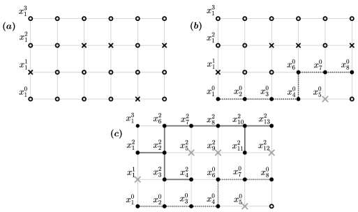
Figure 10.

Appendix B Locations

Claim B.1.

Given $i\in\{{\color[rgb]{0,0,0}2,3}\}$, if $S_{1}\cap\cdots\cap S_{i}$ occurs, then $b^{(i)}+T_{i}(m,n)\subset B({\color[rgb]{0,0,0}(i+1)}Ne_{1},N)$.

Proof.

Let $x\in(b^{(i)}+T_{i}(m,n))$. Then by (54) $x_{1}\in(b_{1}^{(i)}+N+[-m,m])={\color[rgb]{0,0,0}i}N+N+[-m,m]\subset{\color[rgb]{0,0,0}(i+1)}N+[-N,N]$. Using again (54), for $j\geq 2$ we get the following cases: (a) if $b_{j}^{(i)}\geq 0$, then $x_{j}\in[b_{j}^{(i)}-n,b_{j}^{(i)}]\subset[-n,n-m]\subset[-N,N]$; (b) if $b_{j}^{(i)}<0$, then $x_{j}\in[b_{j}^{(i)},b_{j}^{(i)}+n]\subset[-n+m,n]\subset[-N,N]$. ∎

Claim B.2.

If $S_{1}\cap\cdots\cap S_{{\color[rgb]{0,0,0}4}}$ occurs, then $b^{({\color[rgb]{0,0,0}4})}+\hat{T}_{1}(m,n)\subset B(5Ne_{1},N)$, $b^{({\color[rgb]{0,0,0}4})}+\hat{T}_{2}(m,n)\subset B(4Ne_{1}+Ne_{2},N)$ and $b^{({\color[rgb]{0,0,0}4})}+\hat{T}_{3}(m,n)\subset B(4Ne_{1}-Ne_{2},N)$.

Proof.

The inclusion concerning $b^{({\color[rgb]{0,0,0}4})}+\hat{T}_{1}(m,n)$ can be derived as in the proof of Claim B.1. Consider now $x\in(b^{({\color[rgb]{0,0,0}4})}+\hat{T}_{r}(m,n))$ for $r\in\{2,3\}$. Then by (54) with $i={\color[rgb]{0,0,0}4}$ we get that $x_{1}\in b_{1}^{({\color[rgb]{0,0,0}4})}+[0,n]\subset 4N+[-N,N]$ and (a) $x_{2}\in b_{2}^{({\color[rgb]{0,0,0}4})}+N+[-m,m]\subset N+[-n,n]$ for $r=2$; (b) $x_{2}\in b_{2}^{({\color[rgb]{0,0,0}4})}-N+[-m,m]\subset-N+[-n,n]$ for $r=3$. Using (54) with $i={\color[rgb]{0,0,0}4}$ one finally gets that $|x_{j}|\leq N$ for $j\geq 3$, as in the proof of Claim B.1. ∎

B.0.1. Validity of condition (45) in Section 12.4

The inclusion in (45) is trivially satisfied in all steps. We concentrate only on the second property in (45), concerning disjointness.

To proceed we first recall that (54) holds for $i={\color[rgb]{0,0,0}2,3}$. To get the disjointness in (45) for $i\in\{{\color[rgb]{0,0,0}2,3}\}$ we argue as follows. We observe that $R_{i}\cup\partial R_{i}\subset\cup_{k=0}^{i-1}(B^{\prime}_{k}\cup\partial B_{k}^{\prime})$ and points in $\cup_{k=0}^{i-1}(B^{\prime}_{k}\cup\partial B_{k}^{\prime})$ have their first coordinate not bigger than ${\color[rgb]{0,0,0}i}N+m+1$ (cf. Fig. 8, (52) and (54) for $i-1$ instead of $i$). On the other hand, points in $\tilde{b}_{i}+\bigl{(}T_{i}(n)\cup T_{i}(m,n)\bigr{)}$ have their first coordinate not smaller than ${\color[rgb]{0,0,0}i}N+n-1$ (cf. (54)). Since $n-m>2$ we get that $\tilde{b}_{i}+\bigl{(}T_{i}(n)\cup T_{i}(m,n)\bigr{)}$ and $R_{i}\cup\partial R_{i}$ are disjoint for $i\in\{{\color[rgb]{0,0,0}2,3}\}$.

B.0.2. Validity of condition (45) in Section 12.5

The disjointness of $R_{{\color[rgb]{0,0,0}4}}\cup\partial R_{{\color[rgb]{0,0,0}4}}$ and $\tilde{b}_{{\color[rgb]{0,0,0}4}}+\bigl{(}\hat{T}_{1}(n)\cup\hat{T}_{1}(m,n)\bigr{)}$ follows easily from the fact that $x_{1}\leq(\tilde{b}_{{\color[rgb]{0,0,0}4}})_{1}+m+1$ for points $x$ in the first set, while $x_{1}\geq(\tilde{b}_{{\color[rgb]{0,0,0}4}})_{1}+n-1$ for points $x$ in the second set.

We now show that $R_{{\color[rgb]{0,0,0}4}}\cup\partial R_{{\color[rgb]{0,0,0}4}}$ and $\tilde{b}_{{\color[rgb]{0,0,0}4}}+\bigl{(}\hat{T}_{3}(n)\cup\hat{T}_{3}(m,n)\bigr{)}$ are disjoint (the result for $\tilde{b}_{{\color[rgb]{0,0,0}4}}+\bigl{(}\hat{T}_{2}(n)\cup\hat{T}_{2}(m,n)\bigr{)}$ is similar). Suppose first that $(\tilde{b}_{{\color[rgb]{0,0,0}3}})_{2}\geq 0$. Then $(\tilde{b}_{{\color[rgb]{0,0,0}4}})_{2}\in(\tilde{b}_{{\color[rgb]{0,0,0}3}})_{2}+[-n,{\color[rgb]{0,0,0}-m}]$. By construction, if $x\in R_{{\color[rgb]{0,0,0}4}}$ with $x_{1}\geq 4N-m$, then $x\in\tilde{b}_{{\color[rgb]{0,0,0}3}}+T_{{\color[rgb]{0,0,0}3}}(m,n)$ and therefore $x_{2}\geq(\tilde{b}_{{\color[rgb]{0,0,0}3}})_{2}-n$. Take now $y\in\tilde{b}_{{\color[rgb]{0,0,0}4}}+\bigl{(}\hat{T}_{3}(n)\cup\hat{T}_{3}(m,n)\bigr{)}$. Then $y_{1}\geq(\tilde{b}_{{\color[rgb]{0,0,0}4}})_{1}=4N$ and $y_{2}\leq(\tilde{b}_{{\color[rgb]{0,0,0}4}})_{2}-n+1\leq(\tilde{b}_{{\color[rgb]{0,0,0}3}})_{2}-m-n+1$. Suppose by contradiction that $y\in R_{{\color[rgb]{0,0,0}4}}\cup\partial R_{{\color[rgb]{0,0,0}4}}$. Then there exists $x\in R_{{\color[rgb]{0,0,0}4}}$ such that $|x-y|<1$. This implies that $x_{1}\geq y_{1}-1\geq 4N-1$. Hence, by the initial observations, $x_{2}\geq(\tilde{b}_{{\color[rgb]{0,0,0}3}})_{2}-n$. This last bound, together with $y_{2}\leq(\tilde{b}_{{\color[rgb]{0,0,0}3}})_{2}-m-n+1$ and $|x_{2}-y_{2}|\leq 1$, leads to a contradiction as $m>2$.

Suppose that $(\tilde{b}_{{\color[rgb]{0,0,0}3}})_{2}<0$. Then $(\tilde{b}_{{\color[rgb]{0,0,0}4}})_{2}\in(\tilde{b}_{{\color[rgb]{0,0,0}3}})_{2}+[m,n-m]$. By construction, if $x\in R_{{\color[rgb]{0,0,0}4}}$ with $x_{1}\geq 4N-m$, then $x\in\tilde{b}_{{\color[rgb]{0,0,0}3}}+T_{{\color[rgb]{0,0,0}3}}(m,n)$ and therefore $x_{2}\leq(\tilde{b}_{{\color[rgb]{0,0,0}3}})_{2}+n$. Take $y\in\tilde{b}_{{\color[rgb]{0,0,0}4}}+\bigl{(}\hat{T}_{3}(n)\cup\hat{T}_{3}(m,n)\bigr{)}$. Then $y_{1}\geq(\tilde{b}_{{\color[rgb]{0,0,0}4}})_{1}=4N$ and $y_{2}\geq(\tilde{b}_{{\color[rgb]{0,0,0}4}})_{2}+n-1\geq(\tilde{b}_{{\color[rgb]{0,0,0}3}})_{2}+m+n-1$. Suppose by contradiction that $y\in R_{{\color[rgb]{0,0,0}4}}\cup\partial R_{{\color[rgb]{0,0,0}4}}$. Then there exists $x\in R_{{\color[rgb]{0,0,0}4}}$ such that $|x-y|<1$. This implies that $x_{1}\geq y_{1}-1\geq 4N-1$. Hence, by the initial observations, $x_{2}\leq(\tilde{b}_{{\color[rgb]{0,0,0}3}})_{2}+n$. This last bound, together with $y_{2}\geq(\tilde{b}_{{\color[rgb]{0,0,0}3}})_{2}+m+n-1$ and $|x_{2}-y_{2}|\leq 1$, leads to a contradiction as $m>2$.

Appendix C Derivation of (25) from the bound ${\mathbb{Q}}(N_{M}\geq c_{1}M)\geq 1-e^{-c_{2}M}$ in Section 5

In this appendix we explain in detail how to derive (25) with $k:=4N$ from the bound ${\mathbb{Q}}(N_{M}\geq c_{1}M)\geq 1-e^{-c_{2}M}$ obtained in Section 5. Below $c_{3},c_{4},..$ will be positive constant, independent from $M$ and $L$. Since we are interested in $L$ large enough, without loss we think of $M$ as larger than $3$. To help in following the arguments below, we have provided Figure 11.

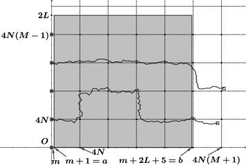
Figure 11. $M=5$, $d=2$. Black circles are points in $\{4N\bar{x}\,:x\in\Lambda\}\subset 4N{\mathbb{Z}}^{d}$. The grey box represent the slice $S$. Paths are in ${\mathbb{G}}_{+}$

Due to the translation invariance of ${\mathbb{P}}$, we can traslate all geometrical objects by the vector $(L+3+m)e_{1}+Le_{2}$. In particular, instead of the slice (24) we will consider the translated one

$$S:=[a,b]\times[0,2L]\times[-4N,4N)^{d-2}\,,\qquad a:=m+1\,,\;b:=2L+5+m\,.$$ (98)

Recall that $\Lambda:=([0,M+1]\times[0,M-1])\cap{\mathbb{Z}}^{2}$ and recall the notation (38). The map $\Lambda\ni x\mapsto 4N\bar{x}\in 4N{\mathbb{Z}}^{d}$ is our natural immersion of $\Lambda$ into the rescaled lattice $4N{\mathbb{Z}}^{d}$. The right vertical face of $\Lambda$ is then mapped inside the set $\{x\in{\mathbb{Z}}^{d}\,:\,x_{1}=4N(M+1)\}$. Recall that $M$ is the minimal integer such that

$$4N(M+1)>b+N\,.$$ (99)

Without loss of generality, when referring to the LR crossings of the box $\Lambda$ for $\zeta$ we restrict to crossings such that only the first and the last points intersect the vertical faces of $\Lambda$ (which would not change the random number $N_{M}$). We fix a set $\Gamma^{\prime}$ of vertex–disjoint LR crossings of $\Lambda$ for $\zeta$ with cardinality $N_{M}$. Then we define $\Gamma$ as the set of paths $(x_{1},x_{2},\dots,x_{k})$ in $\Gamma^{\prime}$ such that $x_{i}$ has second coordinate in $[1,M-2]$ for each $i$ (we stress that the index $i$ here labels points and not coordinates). Note that, since $\Lambda$ is bidimensional, $|\Gamma|\geq|\Gamma^{\prime}|-2$.

Take a LR crossing $(x_{1},x_{2},\dots,x_{k})$ in $\Gamma$. By the discussion in Section 5, we get that there is a path $\gamma$ in ${\color[rgb]{0,0,0}{\mathbb{G}}_{+}}$ from $B(4N\bar{x}_{1},m)$ to $B(4N\bar{x}_{k},N)$ without self-intersections. Moreover, this path is included in the region $\mathcal{R}$ obtained as union of the boxes $B(4N\bar{x}_{i},{\color[rgb]{0,0,0}2N})$ with $i=1,\dots,k$ (see Fig. 8). As the second coordinate of any point $\bar{x}_{i}$ varies in $[1,M-2]$, the second coordinate of any point in $B(4N\bar{x}_{i},{\color[rgb]{0,0,0}2N})$ is in $[4N-2N,4N(M-2)+2N]\subset[0,2L]$. Note that the last inclusion follows from the bound $4NM\leq b+N=2L+5+m+N$ due to the minimality of $M$ in (99). In addition, the box $B(4N\bar{x}_{1},m)$ lies in the halfspace $\{(z_{1},\dots,z_{d})\in\varepsilon{\mathbb{Z}}^{d}\,:z_{1}\leq m\}$, while the box $B(4N\bar{x}_{k},N)$ lies in the halfspace $\{(z_{1},\dots,z_{d})\in\varepsilon{\mathbb{Z}}^{d}\,:z_{1}{\color[rgb]{0,0,0}\geq b+1}\}$ as (99) implies that $4N(M+1)\geq b+N+1$. As a consequence we can extract from the above path $\gamma$ a new path $\tilde{\gamma}$ for ${\color[rgb]{0,0,0}{\mathbb{G}}_{+}}$ lying in $\mathcal{R}\cap\{(z_{1},\dots,z_{d})\in\varepsilon{\mathbb{Z}}^{d}\,:0\leq z_{2}\leq 2L\}\subset\varepsilon{\mathbb{Z}}\times[0,2L]\times[-4N,4N)^{d-2}$, whose first and last points have first coordinate $\leq m$ and $\geq b+1$, respectively.

At cost to further refine $\tilde{\gamma}$, we have that $\tilde{\gamma}$ has the following property $\mathcal{P}$: $\tilde{\gamma}$ is a LR crossing of the box $[a,b]\times[0,2L]\times[-L,L]^{d-2}$ (cf. Definition 3.4) whose vertexes, apart from the first and last one, are contained in $S=[a,b]\times[0,2L]\times[-4N,4N)^{d-2}$, while the first and last one are contained, respectively, in $(-\infty,a)\times[0,2L]\times[-4N,4N)^{d-2}$ and $(b,+\infty)\times[0,2L]\times[-4N,4N)^{d-2}$. Note that the above box is the translated version of the box $\Delta_{L}$ appearing in Proposition 3.6 by the vector $(L+3+m)e_{1}+Le_{2}$, and that one has to translate all geometrical objects by the same vector when applying Definition 3.4.

Moreover, due to the bidimensionality of $\Lambda$, there is an integer $\ell$ (independent from $N,M,L$) such that every path $\tilde{\gamma}$ can share some vertex with at most $\ell$ paths $\tilde{\gamma}^{\prime}$ built in a similar way. Since $M\geq{\color[rgb]{0,0,0}c_{3}}L$ for some $c_{3}>0$, by the above observations we have proved that the event $\{N_{M}\geq{\color[rgb]{0,0,0}c_{1}}M\}$ implies the event $F$ that there are at least $c_{4}L$ vertex–disjoint LR crossings for ${\color[rgb]{0,0,0}{\mathbb{G}}_{+}}$ with the above property $\mathcal{P}$. Hence, by our bound ${\mathbb{Q}}(N_{M}\geq c_{1}M)\geq 1-e^{-c_{2}M}$ and since $M\leq{\color[rgb]{0,0,0}c_{5}}L$, we get that ${\mathbb{Q}}(F)\geq 1-e^{-{\color[rgb]{0,0,0}c_{2}}L}$. Since edges in ${\color[rgb]{0,0,0}{\mathbb{G}}_{+}}$ have length strictly smaller than $1$, the event $F$ does not depend on the vertexes of ${\color[rgb]{0,0,0}{\mathbb{G}}_{+}}$ in $\cup_{s=0}^{M-1}B(4N\bar{x}_{1}^{s},m)$, neither on the edges exiting from the above region. Indeed, by Definition 3.4, to check property $\mathcal{P}$ it would be enough to know the graph ${\mathbb{G}}_{+}$ (vertexes and edges) inside the region $\{(z_{1},\dots,z_{d})\in\varepsilon{\mathbb{Z}}^{d}\,:\,z_{1}>a-1=m\}$. In particular, the event $F$ and the event $D$ defined by (39) are independent, thus implying that ${\mathbb{P}}(F)={\mathbb{P}}(F|{\color[rgb]{0,0,0}D})={\mathbb{Q}}(F)\geq 1-e^{-{\color[rgb]{0,0,0}c_{2}}L}$, and in particular (25) is verified.

Acknowledgements. The authors thank Davide Gabrielli and Vittoria Silvestri for useful discussions. They also thank an anonymous referee for valuable comments improving the presentation of the results.

References

- [1] M. Aizenman, J.T. Chayes, L. Chayes, J. Fröhlich, and L. Russo; On a sharp transition from area law to perimeter law in a system of random surfaces. Comm. Math. Phys. 92, 19–69 (1983).
- [2] V. Ambegoakar, B.I. Halperin, J.S. Langer. Hopping conductivity in disordered systems. Phys, Rev B 4, 2612-2620 (1971).
- [3] D.J. Daley, D. Vere-Jones; An Introduction to the Theory of Point Processes. New York, Springer Verlag, 1988.
- [4] A. Faggionato. Mott’s law for the critical conductance of the Miller–Abrahams random resistor network. Unpublished note, arXiv:1712.07980 (2017).
- [5] A. Faggionato. Miller–Abrahams random resistor network, Mott random walk and 2-scale homogenization. Preprint arXiv:2002.03441 (2020).
- [6] A. Faggionato. Mott’s law for Miller–Abrahams random resistor network and for Mott random walk. In preparation.
- [7] A. Faggionato, P. Mathieu. Mott law as upper bound for a random walk in a random environment. Comm. Math. Phys. 281, 263–286 (2008).
- [8] A. Faggionato, H.A. Mimun. Connection probabilities in Poisson random graphs with uniformly bounded edges. ALEA 16 463–486 (2019).
- [9] A. Faggionato, H. Schulz–Baldes, D. Spehner. Mott law as lower bound for a random walk in a random environment. Comm. Math. Phys., 263, 21–64 (2006).
- [10] P. Gracar, M. Heydenreich, C. Mönch, P. Mörters. Recurrence versus Transience for Weight-Dependent Random Connection Models. Preprint arXiv:1911.04350 (2019).
- [11] G. Grimmett, Percolation. Second edition. Die Grundlehren der mathematischen Wissenschaften 321. Springer Verlag, Berlin, 1999.
- [12] G.R. Grimmett, J.M. Marstrand. The supercritical phase of percolation is well behaved. Proc. R. Soc. Lond. A 430, 439–457 (1990).
- [13] O. Kallenberg. Foundations of modern probability. Second edition. Probability and its Applications, Springer Verlag, Berlin, 2002.
- [14] S. Martineau, V. Tassion. Locality of percolation for Abelian Cayley graphs. Ann. Probab. 45, 1247–1277 (2017).
- [15] R. Meester, R. Roy. Continuum percolation. Cambridge Tracts in Mathematics 119. First edition, Cambridge University Press, Cambridge, 1996.
- [16] A. Miller, E. Abrahams. Impurity Conduction at Low Concentrations. Phys. Rev. 120, 745–755 (1960).
- [17] M. Pollak, M. Ortuño, A. Frydman. The electron glass. First edition, Cambridge University Press, United Kingdom, 2013.
- [18] H. Tanemura. Behavior of the Supercritical Phase of a Continuum Percolation Model on . J. Appl. Prob. 30, 382-396 (1993).