The Integrated Vehicle and Pollster Routing Problem

Abstract

The National Statistics Bureau of Ecuador carries out monthly polls to monitor the evolution of an economic indicator called “Consumer Price Index”, which measures the consumer prices of basic commodities. A set of stores is selected to apply these polls. Furthermore, a set of vehicles transports pollsters from the headquarters of the bureau to the stores to perform this activity. Moreover, pollsters move between stores using pedestrian paths or using a vehicle to shorten the travel time. This paper introduces the Integrated Vehicle and Pollster Routing Problem alongside an integer program to model the integrated task of scheduling visits of pollsters to selected stores, as well as routing the vehicle fleet used to transport them. Results on the computational complexity of the aforementioned problem, a three-phase algorithm, and computational experience based on real-world instances are provided.

1 Introduction

The Vehicle Routing Problem (VRP) is a well-known and complex combinatorial problem, which has received considerable attention since the fifties. Thus, Dantzig and Ramser (1959) formally introduced the Vehicle Routing Problem as a generalization of the Traveling Salesman Problem, where a simple matching-based heuristic for its solution was proposed. A few years later, Clarke and Wright (1964) developed one of the most used approaches for this problem with an iterative procedure that enables the rapid selection of an optimal or near-optimal route. Iterative search methods (Taillard, 1993; Gendreau et al., 1994; Osman, 1993) can be adapted easily to problems dealing with a large number of constraints, although they require considerable computing times and several parameter settings. Seminal concepts for exact methods appear successfully in the eighties, where Christofides et al. (1981) proposed tree search algorithms incorporating lower bounds computed from shortest spanning $k$-degree centre tree and $q$-paths. Also, Laporte et al. (1984) proposed the Gomory cutting planes and branch and bound approaches based on an integer formulation. Since then, different applications of the VRP have been reported in (Gracia et al., 2014; Linfati et al., 2018; Chowmali and Sukto, 2020) as well as a variety of exact algorithms (Baldacci et al., 2007; Florio et al., 2020), heuristics, and metaheuristics (Pisinger and Ropke, 2007; Vidal et al., 2013; Toffolo et al., 2019; Cordeau et al., 2005).

The routing problem treated in this work arises from two well-established variants of the VRP: the Pickup & Delivery Problem (PDP) and the Dial-a-Ride Problem (DARP). These problems have been studied using many different approaches including both exact and heuristic methods.

On the one hand, PDP constitutes a relevant subset of routing problems in which commodities or passengers have to be transported from different origins to many other destinations. Savelsbergh and Sol (1995) discussed several characteristics that distinguish the PDP from standard VRPs and presented a survey of these problems and solution methods. In similar way, Parragh et al. (2008a) focused on routing problems involving pickups and deliveries related with the transportation of goods from the depot to line-haul customers and from back-haul customers to the depot. Ferrucci (2013) considered that clients can be seen as intermediaries which can also return goods. Sartori and Buriol (2018) solved the PDP using a matheuristic based on the Iterated Local Search method with an embedded Set Partitioning Problem that is iteratively solved to recombine routes of previously found solutions. Furtado et al. (2017) proposed a modeling strategy that allows the assignment of vehicles to routes explicitly in two-index flow formulations. Extensive surveys on this problem concerning exact and heuristic approaches are available at (Parragh et al., 2008b, c; Battarra et al., 2014; Doerner and Salazar-González, 2014).

On the other hand, the DARP can be considered itself as a generalization of the PDP and the VRP with Time Windows, since it consists of designing vehicle routes and schedules for individual persons who specify pickup and delivery requests. The most common application can be found in door-to-door transportation services (Melachrinoudis et al., 2007; Borndörfer et al., 1999). Furthermore, Madsen et al. (1995) presented a problem which is characterized by multiple capacities and multiple objectives describing a system for the solution of a static Dial-a-Ride routing and scheduling problem with time windows. Braekers et al. (2014) introduced a branch-and-cut algorithm for the standard DARP which is adapted to exactly solve small problem instances of the Multi-Depot Heterogeneous DARP. In Coslovich et al. (2006), a dynamic DARP with time window constraints together with a two-phase insertion algorithm based on route perturbations is considered. If transportation requests of users between a set of pickup points and a set of delivery points are considered, Masson et al. (2014) provided a solution method based on an Adaptive Large Neighborhood Search metaheuristic and explained how to check the feasibility of a request insertion. Complete surveys on DARP can be found in Ho et al. (2018); Molenbruch et al. (2017); Cordeau and Laporte (2003).

Joint vehicle and crew routing and scheduling problems are also reported in the literature. Thus, Lam et al. (2020) introduced a problem in which crews are able to interchange vehicles, resulting in space and time interdependencies between vehicle routes and crew routes. It proposes a constraint programming model that overlays crew routing constraints over a standard VRP. In Fikar and Hirsch (2015), a project motivated by the Austrian Red Cross is proposed. Here, a solution procedure for the daily planning of home healthcare providers that operate multiple vehicles to deliver nurses to clients and to pick them up after service is provided. Moreover, the authors introduced a matheuristic consisting of two stages, identifying potential walking-routes and optimising the transport system. Molenbruch et al. (2021) introduced a routing algorithm and integrated scheduling procedure to enforce the synchronization of flexible vehicle routes to timetables of the remaining public transport services, enabling the design and operational implementation of an integrated mobility system. In the same context, Drexl et al. (2013) studied a simultaneous vehicle and crew routing and scheduling problem arising in long-distance road transport in Europe; a solution heuristic based on a two-stage decomposition of the problem is developed, taking into account European Union social legislation for drivers.

This paper focuses on a version of the joint vehicle and crew routing and scheduling problem. The problem arises from data collection procedures designed at the National Statistics Bureau of Ecuador (INEC) to compute the national Consumer Price Index. A group of pollsters and a fleet of vehicles traverse shared pedestrian and vehicular routes in order to visit a set of stores scattered throughout the city of Guayaquil and its outskirts in several days. Each store is visited by a pollster to collect the prices of specific goods needed to calculate the aforementioned index. Furthermore, pollsters can either walk or be transported by vehicles of fixed capacity through a workday with morning and afternoon shifts, separated by a mandatory break. Every vehicular route must begin at INEC headquarters dropping and picking up pollsters along the way, allowing vehicles to be back or wait at each store. At the end of each workday, vehicles and pollsters must return to the headquarters. The objective of this problem aims to reduce the sum of fixed and variable daily-costs. The former are associated to the maintenance of the depot, and the latter are related to hiring pollsters and vehicles.

This paper makes several contributions to the vast literature of Transportation Problems. First, a problem which is a variation of the General Pick-up and Delivery Problem (GPDP) and the Dial-a-Ride Problem (DARP) is proposed. Unlike the GPDP, where transhipments at intermediate locations and autonomous load movements are not allowed, it considers the possibility that a pollster, left at a specific node to perform a task, might be picked-up by another vehicle; a pollster can also move through the network from one node to another using a pedestrian route. Thus, transhipments and autonomous transportation of the freight are included in this model. This fact reveals the need of syncing vehicular and pedestrian routes respecting a maximum arrival time corresponding to the length of a working day. Second, this research studies the problem’s complexity, proving that it is $\mathcal{NP}$ – hard. The latter result leads to some modeling, algorithmic, and computational challenges which have been adequately overcome using Integer Programming tools together with a three-phase heuristic. Finally, the results presented in this study help provide a better understanding of the pollstering logistic processes for a public institution and a considerably reduction of operational costs of up to 50%.

The structure of this paper is given as follows: in Section 2 an IP-based formulation for the Integrated Vehicle and Pollster Routing Problem is introduced along with the proof of its computational complexity. Due to the hardness of the problem, Section 3 presents a three-phase heuristic. Afterwards, a real-world instance together with computational results are described in Section 4. Finally, in Section 5, concluding remarks are reported.

2 An integrated model for routing pollsters and vehicles

2.1 Notation

Let $S$ be the set of days of a planning horizon. For each store and for the sake of modeling simplification, let $C:=C_{-}\cup C_{+}$ be the set of stores that have to be visited on some day $s\in S$, where $C_{-}:=\{1,\dots,n\}$ corresponds to the set of nodes associated to each store and $C_{+}:=\{n+1,\dots,2n\}$ is a set of copies of the nodes in $C_{-}$ as depicted in Figure 1. In this problem, due to technical requirements, only one depot is considered. It is assumed that pollsters must depart and arrive in a vehicle on a daily basis. The depot and its copy are denoted by nodes $0$ and $2n+1$, from which pollsters and vehicles depart and arrive, respectively. Node-duplication allows to model vehicle arrival, service, waiting, and departure times, separately.

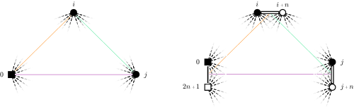
Figure 1: Node-duplication

Let $G:=(V,A)$ be a multi-graph where the node set is $V:=C\cup\{0,2n+1\}$, and the arc set $A:=A_{S}\cup A_{W}\cup A_{V}$ contains three different kinds of arcs. The first group $A_{S}:=\big{\{}(i,i+n):i\in C_{-}\big{\}}$ is the set of arcs which connect every store with its duplicate; they are called service arcs. The second group of arcs $A_{W}:=\big{\{}(i,j):i\in C_{+},j\in C_{-},i\neq j+n\big{\}}$, called walking arcs, links every pair of stores. Finally, the vehicle transportation arc set, $A_{V}:=\big{\{}(i,j):i,j\in C,i\neq j,i\neq j+n\big{\}}\cup\{(0,i):i\in C_{-}\big{\}}\cup\big{\{}(i,2n+1):i\in C_{+}\big{\}}$ represents potential connections between nodes or depots using vehicles. Moreover, for every arc $a\in A_{S}$, the parameter $t_{a}>0$ is the time spent by a pollster collecting data at a store; for each arc $a\in A_{W}$, $t_{a}>0$ is the pedestrian travel time between stores, and, for $a\in A_{V}$, $\tau_{a}\geq 0$ is the vehicular travel time between two nodes ($\tau_{a}=0$ only if $a\in A_{S}$). A representation of the resulting multigraph is displayed in Figure 2.

Visits are carried out by a set $E$ of pollsters which are transported by a homogeneous fleet of vehicles $K$ with positive integer capacity $Q$. Each operational day has an associated fixed cost of $\kappa_{0}\geq 0$. Similarly, vehicles and pollsters have a fixed hiring cost of $\kappa_{1}\geq 0$ and $\kappa_{2}\geq 0$, respectively, and they work within a daily time frame $[0,B_{\max}]$. Due to labor regulations, pollsters must take a break of $P\geq 0$ minutes starting in the time interval $[T_{0},T_{1}]\subset[0,B_{\max}-P]$.

A vehicular route is a simple path from node $0$ to $2n+1$ using exclusively arcs in $A_{V}$. A pedestrian route, also called walking path, is a simple path from $i\in C_{-}$ to $j\in C_{+}$ consisting of an alternating sequence of arcs in sets $A_{S}$ and $A_{W}$. A feasible service route for a pollster is defined as a simple path from $0$ to $2n+1$ linking pedestrian routes with segments of vehicular routes. Thus, at every node $i$, a pollster stays $t_{i,i+n}$ units of time to accomplish a task respecting the maximum daily duty length. At last, a feasible daily plan consists in different feasible service routes synced according to the duration of each pedestrian and vehicular route, and any sequence of feasible daily plans forms an aggregated daily plan.

The Integrated Vehicle and Pollster Routing Problem (IVPRP) consists in finding an aggregated daily plan to visit every node $i\in C$ exactly once at minimum cost. This plan must hire at most $|K|$ vehicles of capacity $Q$ and $|E|$ pollsters in no more than $|S|$ days. The IVPRP is $\mathcal{NP}$ – hard as proved in the following theorem.

Theorem 2.1

The IVPRP is $\mathcal{NP}$ – hard.

Proof

Proof: The $\mathcal{NP}$ – hardness is proved by using a polynomial transformation from the Traveling Salesman Problem (TSP). Let $K_{n+1}$ ($n\geq 3$) a complete graph with set of nodes $\{0,1,\dots,n\}$ with weights $c:E(K_{n+1})\to\mathbb{R}_{+}$. An instance of the IVPRP is constructed as follows: an arbitrary node in $V(K_{n+1})$ is chosen as the depot. Without loss of generality let $0$ be such a node. The remaining nodes in $V(K_{n+1})$ correspond to every store of our problem, i.e., $C:=C_{-}\cup C_{+}$ with $C_{-}=V(K_{n+1})\setminus\{0\}$ and the multigraph $D$ is constructed as above. The cost function $c$ in the TSP corresponds to the vehicular travel times $\tau$ for arcs $(i,j)$, $i,j\in C$, $i\neq j$ in $A_{V}$ and $0$ otherwise. Pedestrian travel time $t_{a}\gg\sum_{a\in A_{V}}\tau_{a}$ and $t_{a}=0$ for $a\in A_{S}$. Moreover, fix $|E|=|K|=|S|=1$, $Q=1$, $P=0$, $B_{\max}=\infty$, and the break time window is set to $[0,B_{\max})$.

If the Hamiltonian cycle $\{0,i,j,k,\dots,0\}$ is a feasible solution of the TSP with cost $H$, then IVPRP has a feasible solution with the same cost given by the vehicular route $\{0,i,i+n,j,j+n,k,k+n,\dots,2n+1\}$, the pedestrian route $\bigcup_{i\in C_{-}}(i,i+n)$, and both forming a service route which is also a feasible daily plan. Conversely, suppose that the IVPRP has a feasible solution with an aggregated daily plan of length less than $\sum_{a}\tau_{a}$. Since the pedestrian travel times are larger than $\sum_{a}\tau_{a}$, then the pedestrian arcs in $A_{W}$ are never used in that solution. Thus, the feasible service route reveals a Hamiltonian cycle for the TSP with the same cost.

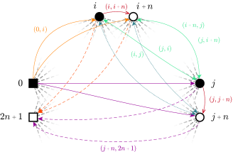
Figure 2: Multigraph construction for the IVPRP

2.2 Formulation

For the sake of simplicity, the integrated vehicle and pollster routing model (IVPRM) is stated in the following blocks.

Variables

The following sets of binary variables for arc selection are used in the model. First, variable $x_{i,j}^{e,s}$ is equal to one if and only if the arc $(i,j)\in A_{S}\cup A_{W}$ is chosen to be part of some walking path of the pollster $e\in E$ on day $s\in S$. Second, $y_{i,j}^{k,s}$ is one whenever arc $(i,j)\in A_{V}$ is part of the route of vehicle $k\in K$ on day $s\in S$. Third, $z_{i,j}^{e,s}$ indicates if pollster $e\in E$ is transported by some vehicle over arc $(i,j)\in A_{V}$ on day $s\in S$. Fourth, $b_{i}^{e,s}$ (correspondingly $f_{i}^{e,s}$) indicates if a pollster $e\in E$ starts (finishes) a walking path at node $i\in C_{-}$ ($i\in C_{+}$) on day $s\in S$. Fifth, $w_{i}^{e,s}$ indicates if a pollster $e\in E$ takes a break at node $i\in C_{-}$ on day $s\in S$. At last, $u_{s}$ determines if any workload is assigned to pollsters and vehicles on day $s\in S$ for the final aggregated daily plan. Additionally, for each node $i\in C_{-}$, let us define $B_{i}$ and $B_{i+n}$ as the arrival and departure times of a pollster at nodes $i$ and $i+n$, respectively.

Objective function

The objective function aims to minimize the number of operational days and the number of vehicles and pollsters hired. The first component represents the fixed operational daily cost meanwhile the other two components represent the variable costs depending on the number of pollsters and vehicles hired for an operational day. In despite of the fact that this definition of an objective function is not frequent in Routing Problems, this is justified because the distance walked by a pollster, or the travel time spent by a vehicle, are not relevant quantities for this particular application (fixed daily costs of hiring vehicles and pollsters).

$$\min\,\kappa_{0}\,\sum_{s\in S}u^{s}+\kappa_{1}\,\sum_{s\in S}\sum_{k\in K}\sum_{j\in C}y_{0,j}^{k,s}+\kappa_{2}\,\sum_{s\in S}\sum_{e\in E}\sum_{j\in C}z_{0,j}^{e,s}.$$ (1)

Pollster routing

The following set of constraints describe routes for each pollster $e\in E$ within each day $s\in S$ in the time horizon.

$$\displaystyle\sum_{s\in S}\sum_{e\in E}x_{i,i+n}^{e,s} =1 \forall i\in C_{-},$$ (2a)

$$\displaystyle\sum_{j\in C_{+}}x_{j,i}^{e,s}-x_{i,i+n}^{e,s} =-b_{i}^{e,s} \forall i\in C_{-},e\in E,s\in S,$$ (2b)

$$x_{i-n,i}^{e,s}-\displaystyle\sum_{j\in C_{-}}x_{i,j}^{e,s} =f_{i}^{e,s} \forall i\in C_{+},e\in E,s\in S,$$ (2c)

$$\sum_{j\in C\cup\{0\}}z_{j,i}^{e,s} \leq 1-x_{i,i+n}^{e,s}+b_{i}^{e,s} \forall i\in C_{-},e\in E,s\in S,$$ (2d)

$$\sum_{j\in C\cup\{2n+1\}}z_{i,j}^{e,s} \leq 1-x_{i-n,i}^{e,s}+f_{i}^{e,s} \forall i\in C_{+},e\in E,s\in S,$$ (2e)

$$\displaystyle\sum_{j\in C\cup\{0\}}z_{j,i}^{e,s}\quad-\sum_{j\in C\cup\{2n+1\}}z_{i,j}^{e,s} =b_{i}^{e,s} \forall i\in C_{-},e\in E,s\in S,$$ (2f)

$$\displaystyle\sum_{j\in C\cup\{0\}}z_{j,i}^{e,s}\quad-\sum_{j\in C\cup\{2n+1\}}z_{i,j}^{e,s} =-f_{i}^{e,s} \forall i\in C_{+},e\in E,s\in S,$$ (2g)

$$\sum_{i\in C}z_{0,i}^{e,s} \leq u_{s} \forall e\in E,s\in S.$$ (2h)

Constraints (2a) ensure that each store $i\in C_{-}$ is visited exactly once by a pollster on a given day. Constraints (2b) and (2c) identify the edges of walking paths, i.e., if $b_{i}^{e,s}=1$ (resp. $f_{i}^{e,s}=1$), then a walking path must begin (resp. end) at node $i\in C_{-}$ (resp. $C_{+}$). Moreover, constraints (2d) – (2g) guarantee that if a node $i$ is the beginning or the end of a walking path, then exactly one vehicle must pick up or deliver exactly one pollster on that node. Finally, constraints (2h) enforce that each pollster leaves the depot at most once in every active day.

Vehicle routing

The following constraints characterize vehicular routes for pollster transportation.

$$\displaystyle\sum_{k\in K}\sum_{j\in C\cup\{2n+1\}}y_{i,j}^{k,s} =\sum_{e\in E}b_{i}^{e,s} \forall i\in C_{-},\,\forall s\in S,$$ (3a)

$$\displaystyle\sum_{k\in K}\sum_{j\in C\cup\{2n+1\}}y_{i,j}^{k,s} =\sum_{e\in E}f_{i}^{e,s} \forall i\in C_{+},\,\forall s\in S,$$ (3b)

$$\sum_{i\in C\cup\{0\}}y_{i,j}^{k,s}\quad-\sum_{i\in C\cup\{2n+1\}}y_{j,i}^{k,s} =0 \forall j\in C,k\in K,s\in S,$$ (3c)

$$\displaystyle\sum_{j\in C}y_{0,j}^{k,s}-\sum_{j\in C}y_{j,2n+1}^{k,s} =0 \forall k\in K,s\in S,$$ (3d)

$$\sum_{i\in C}y_{0,i}^{k,s} \leq u_{s} \forall k\in K,s\in S,$$ (3e)

$$\sum_{e\in E}z_{i,j}^{e,s} \leq Q\sum_{k\in K}y_{i,j}^{k,s} \forall(i,j)\in A,s\in S.$$ (3f)

Constraints (3a) and (3b) ensure that vehicles arrive only to pick up nodes and depart just from delivery nodes. (3c) and (3d) are flow conservation constraints. Furthermore, (3e) determine that each vehicle leaves the depot at most once in every active day. Finally, (3f) establish the linkage between pollster and vehicular routes.

Time management and shift-length

The set of constraints below are introduced to describe time bounds for the duration of a pollster shift and times required to travel and visit each store.

$$B_{i+n}\geq B_{i}+t_{i,i+n}+P\sum_{s\in S}\sum_{e\in E}w_{i}^{e,s} \forall i\in C_{-},$$ (4a)

$$B_{j}\geq B_{i}+t_{i,j}-M\bigg{(}1-\sum_{s\in S}\sum_{e\in E}x_{i,j}^{e,s}\bigg{)} \forall i\in C_{+},j\in C_{-},$$ (4b)

$$B_{j}\geq B_{i}+\tau_{i,j}-M\bigg{(}1-\sum_{s\in S}\sum_{k\in K}y_{i,j}^{k,s}\bigg{)} \forall(i,j)\in A_{V},i\neq 0,j\neq 2n+1,$$ (4c)

$$B_{i}\geq\tau_{0,i}-M\bigg{(}1-\sum_{s\in S}\sum_{k\in K}y_{0,i}^{k,s}\bigg{)} \forall i\in C,$$ (4d)

$$B_{\max}u_{s}\geq B_{i}+\tau_{i,2n+1}-M\left(1-\sum_{k\in K}y_{i,2n+1}^{k,s}\right) \forall i\in C,s\in S,$$ (4e)

Constraints (4a) require that the departure time from a store $i$ to be at least as large as the arrival time plus the service time and, eventually, the time needed in case a pause is taken at that store. Observe that the sum in the right-most term in these constraints equals one if a pause is taken at node $i$ and zero otherwise. Constraints (4b) and (4c) ensure that the arrival time at a store, within a route, must include the pedestrian or vehicular travel time from the previous visited store, respectively. If node $i$ comes right after the depot in any route, then constraints (4d) provide a lower bound on the arrival time of vehicles and pollsters. Finally, constraints (4e) link variables $B_{i}$ and $u^{s}$ in order to bound the latest arrival time of any vehicle to the depot for each day $s$. Here, $M$ is a sufficiently large number such that $M>\max\{t,\tau\}+B_{\max}$.

Pollster breaks

The subsequent constraints ensure that each pollster on duty must take a break starting within the prescribed time frame on a given day.

$$T_{0}\sum_{s\in S}\sum_{e\in E}w_{i}^{e,s}\leq B_{i}+t_{i,i+n}\leq T_{1}+M\bigg{(}1-\sum_{s\in S}\sum_{e\in E}w_{i}^{e,s}\bigg{)} \forall i\in C_{-},$$ (5a)

$$w_{i}^{e,s}\leq x_{i,i+n}^{e,s} \forall i\in C_{-},e\in E,s\in S,$$ (5b)

$$\sum_{i\in C_{-}}w_{i}^{e,s}=\sum_{j\in C}z_{0,j}^{e,s} \forall e\in E,s\in S.$$ (5c)

Constraints (5a) establish that if a break is taken by a pollster at node $i$, then it must occur within the time interval $[T_{0},T_{1}]$. Constraints (5b) guarantee that a pollster takes a break only at visited stores, and constraints (5c) enforce that each pollster on duty takes a break once per day.

2.3 Symmetry breaking inequalities

In any feasible aggregated daily plan, there is a fixed vehicle which serves a vehicular route, yet the route can be served by any other vehicle in $K$, yielding the same objective value. In the same manner, the workload of any pair of pollsters in $E$ can be permuted throughout a daily plan. Moreover, the same happens with the set of days $S$ in relation with the feasible daily plans. Then, a set of equivalent solutions might appear by relabeling assigned vehicles and pollsters. The following set of constraints try to avoid these symmetries. This can be seen as an application of the well known technique of symmetries elimination (Kaibel et al., 2011; Ostrowski et al., 2009; Margot, 2009).

$$\sum_{i\in C}z_{0,i}^{0,0}=1,$$ (6a)

$$\sum_{i\in C}z_{0,i}^{e,s}\leq\sum_{i\in C}z_{0,i}^{e-1,s}, \forall e\in E\setminus\{0\},s\in S,$$ (6b)

$$\sum_{i\in C}z_{0,i}^{e,s}\leq\sum_{i\in C}z_{0,i}^{e,s-1}, \forall e\in E,s\in S\setminus\{0\},$$ (6c)

$$\sum_{i\in C}y_{0,i}^{0,0}=1,$$ (6d)

$$\sum_{i\in C}y_{0,i}^{k,s}\leq\sum_{i\in C}y_{0,i}^{k-1,s}, \forall k\in K\setminus\{0\},s\in S,$$ (6e)

$$\sum_{i\in C}y_{0,i}^{k,s}\leq\sum_{i\in C}y_{0,i}^{k,s-1}, \forall k\in K,s\in S\setminus\{0\},$$ (6f)

$$\sum_{e\in E}b_{i}^{e,s}\leq 1-\sum_{e\in E}b_{i}^{e,s-1}, \forall i\in C_{-},s\in S\setminus\{0\},$$ (6g)

$$\sum_{e\in E}f_{i}^{e,s}\leq 1-\sum_{e\in E}f_{i}^{e,s-1}, \forall i\in C_{+},s\in S\setminus\{0\},$$ (6h)

$$\displaystyle\sum_{e\in E}\sum_{j\in C_{+}}x_{j,i}^{e,s}\leq 1-\sum_{e\in E}b_{i}^{e,s-1}, \forall i\in C_{-},s\in S\setminus\{0\},$$ (6i)

$$\displaystyle\sum_{e\in E}\sum_{j\in C_{-}}x_{i,j}^{e,s}\leq 1-\sum_{e\in E}f_{i}^{e,s-1}, \forall i\in C_{+},s\in S\setminus\{0\},$$ (6j)

$$\sum_{i\in C_{-}}b_{i}^{e,s}\leq|C_{-}|-\sum_{r=0}^{s-1}\sum_{i\in C_{-}}b_{i}^{e-1,r}, \forall e\in E\setminus\{0\},s\in S\setminus\{0\},$$ (6k)

$$\sum_{i\in C_{+}}f_{i}^{e,s}\leq|C_{+}|-\sum_{r=0}^{s-1}\sum_{i\in C_{+}}f_{i}^{e-1,r}, \forall e\in E\setminus\{0\},s\in S\setminus\{0\},$$ (6l)

$$u^{s}\leq u^{s-1}, \forall s\in S\setminus\{0\}.$$ (6m)

Constraints (6a) – (6c) ensure an ordered assignment of pollsters starting with the one labeled as $0$ for each day $s\in S$. Similarly, constraints (6d) – (6f) guarantee an ordered assignment for vehicles. Constraints (6g) – (6j) define daily relationships between served stores in two consecutive days, i.e., if node $i$ is visited at day $s-1$, then the related variables to this node at day $s$ are bounded to zero. (6k) – (6l) impose an upper bound on the number of stores that were not visited in the previous days. At last, constraints (6m) reinforce consecutive active days.

2.4 Upper bounds

An upper bound for the objective function of IVPRP can be obtained by solving the following nonlinear problem:

$$\min\kappa_{0}\ell_{S}+\kappa_{1}\ell_{K}\ell_{S}+\kappa_{2}\ell_{E}\ell_{S}$$ (7a)

subject to

$$\dfrac{1}{\ell_{E}}\Big{(}P\ell_{E}\ell_{S}+\sum_{i\in C_{-}}t_{i,i+n}\Big{)}+\dfrac{1}{\ell_{K}}\sum_{i\in V}\big{(}\max\{\tau_{i,j}:(i,j)\in A_{V}\}+\max\{\tau_{j,i}:(j,i)\in A_{V}\}\big{)}\leq B_{\max}\ell_{S},$$ (7b)

$$\ell_{K}\leq\ell_{E}\leq Q\ell_{K},$$ (7c)

$$1\leq\ell_{S}\leq|S|,$$ (7d)

$$1\leq\ell_{K}\leq|K|,$$ (7e)

$$1\leq\ell_{E}\leq|E|,$$ (7f)

$$\ell_{S},\ell_{K},\ell_{E}\in{\mathbb{Z}}^{+};$$ (7g)

where $\ell_{S}$, $\ell_{K}$, and $\ell_{E}$ are decision variables representing the number of needed days, vehicles, and pollsters, respectively. The optimal solution $(\ell_{S}^{*},\ell_{K}^{*},\ell_{E}^{*})$ of (7a)–(7f) provides an upper bound on the objective function (1) of model IVPRM. As a result, this solution determines a tighter value on the cardinality of sets $S$, $K$, and $E$ required to get an aggregated daily plan.

Observe that constraint (7b) distributes a day in two portions. On the one hand, the first term averages the pollstering time, plus breaks, that each pollster would take on all days to finish an aggregated daily plan. On the other hand, the second term averages the time required, on a worst case scenario, to travel by vehicle to leave pollsters and pick them up at each node. The sum of both terms in any feasible solution for IVPRM necessarily has to be below the time horizon $B_{\max}$. Furthermore, constraint (7c) bounds the number of pollsters by vehicle capacity. At last, the optimal solution can be obtained, in the worst case, using exhaustive enumeration in $\mathcal{O}\big{(}|S||K||E|\big{)}$ time.

2.5 Lower bounds

Likewise, it is possible to determine lower bounds from store visiting times. To do so, first let $\ell_{e}$ be the lowest integer value that represents the minimum number of pollsters required, in at most $|S|$ days, to distribute the aggregated service time with respect to the maximum shift and mandatory break lengths. This value is obtained by solving the nonlinear program

$$\max\big{\{}\frac{1}{\ell_{e}}\sum_{i\in C_{-}}t_{i,i+n}:\,\frac{1}{\ell_{e}}\sum_{i\in C_{-}}t_{i,i+n}\leq B_{\max}-P\wedge\ell_{e}\in\{1,\ldots,|S||E|\}\big{\}}.$$ (8)

Notice that if problem (8) is infeasible, then there are not enough resources to solve IVPRM; thus, providing an infeasibility certificate.

Next, the minimum number of days required to visit all stores, noted $\ell_{s}$, is recovered as the first index $s$ such that $\ell_{e}$ belongs to the set $\Lambda_{E,s}=\{s,s+1,\ldots,s\cdot|E|\}$ for all $s\in\{1,\ldots,|S|\}$. Here $\Lambda_{E,s}$ is the set containing the cumulative number of pollsters that can be active on a day with index $s$.

At last, a bound on the number of vehicles is derived by observing that if a day is active then there must be an active vehicle as well (see (3f)), and that each vehicle can transport at most $Q$ pollsters. Thus the smallest number $\ell_{k}$ that satisfies these constraints solves the following linear program: $\min\big{\{}\ell_{k}:\,\ell_{e}\leq Q\ell_{k}\,\wedge\,\ell_{k}\in\{\ell_{s},\ldots,\ell_{s}|K|\}\big{\}}$.

A solution for these three problems can be obtained with exhaustive enumeration in $\mathcal{O}\big{(}|S||E|+|K|\big{)}$ time. Moreover, while the upper bounds $(\ell_{S},\ell_{K},\ell_{E})$ would change according to the costs in the objective function, the lower bounds $(\ell_{s},\ell_{k},\ell_{e})$ are cost-independent. They are added to IVPRM as the following constraints:

$$\sum_{s\in S}u^{s} \geq\ell_{s},$$ (9a)

$$\sum_{s\in S}\sum_{k\in K}\sum_{j\in C}y_{0,j}^{k,s} \geq\ell_{k},$$ (9b)

$$\sum_{s\in S}\sum_{e\in E}\sum_{j\in C}z_{0,j}^{e,s} \geq\ell_{e}.$$ (9c)

These result in the lower bound $\kappa_{0}\ell_{s}+\kappa_{1}\ell_{k}+\kappa_{2}\ell_{e}$ with respect to the objective of IVPRM.

2.6 An illustrated example

In order to explain the solution approach for the IVPRP, a small instance is presented in Figure 3 with the following parameters: $n=4$ stores, $|E|=2$ pollsters, $|K|=2$ vehicles with capacity $Q=2$, and a limit of $|S|=2$ days; the break is fixed to one minute within a time frame of $[T_{0},T_{1}]=[20,30]$; the time horizon is set to 30 minutes, the fixed and variable costs are $\kappa_{0}=\$300$, $\kappa_{1}=\$100$, and $\kappa_{2}=\$80$, respectively. The vehicular and pedestrian travel times are shown in Table 1. The diagonal of the pollster travel time matrix corresponds to the service times. Observe that this table does not contain information related to nodes in the set $\{5,6,7,8,9\}$ which are the duplicated nodes explained in the multigraph construction.

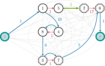
Figure 3: Multigraph and optimal solution for an IVPRP instance

Table 1: Time parameters

		Vehicle					Pollster
		$0$	$1$	$2$	$3$	$4$	$1$	$2$	$3$	$4$
Store	$0$	–	$1$	$4$	$6$	$2$	–	–	–	–
	$1$	$2$	–	$1$	$2$	$10$	$1$	$2$	$3$	$14$
	$2$	$1$	$1$	–	$4$	$15$	$2$	$17$	$8$	$20$
	$3$	$7$	$2$	$5$	–	$9$	$3$	$8$	$1$	$15$
	$4$	$1$	$15$	$11$	$9$	–	$15$	$20$	$15$	$1$

As portrayed in Figure 3, the optimal solution for this small instance consists of one vehicular route: $0\to 1\to 4\to 8\to 3\to 7\to 6\to 9$ (continuous lines); three pedestrian routes: $1\to 5\to 2\to 6$ for pollster $0$, and $4\to 8$ and $3\to 7$ for pollster $1$. Synced pedestrian and vehicular routes form feasible service routes corresponding to the optimal daily plan. Breaks are represented by dashed nodes $2$ and $3$ for pollster 0 and 1, respectively. The optimal value is accomplished in one day using one vehicle and two pollsters with a total cost of $\$560$.

3 Solution approach

3.1 Three-phase Algorithm

Given that the IVPRP is $\mathcal{NP}$ – hard, preliminary tests have shown that finding an optimal solution for instances with even a small number of nodes is not guaranteed in a reasonable time. Thus, a heuristical procedure is proposed in this subsection. The method consists of three phases which are solved consecutively. In the first phase, the set of nodes is partitioned into an even number of balanced subsets where each partition is associated to a part-time daily plan, whether in the morning or in the afternoon, without breaks. The second phase takes the graph induced by the nodes of each partition as an input and solve IVPRM problem. This input-reduced version of the main problem is notated by (R-IVPRM). The last phase links adequately the solutions found for each partition to obtain feasible daily plans. Other approaches using graph-partitioning techniques have been similarly reported in the literature; see (Sartori and Buriol, 2018; Alvarenga and Mateus, 2004).

Partitioning

In order to separate the node set into smaller-size subsets, the following problem is solved: let $G=(C_{-},F)$ be an undirected complete graph with costs on the edges, which coincides with the pedestrian travel times between each pair of stores. Also, let $t:C_{-}\longrightarrow\mathbb{R}^{+}$ a weight function representing service times at stores, and let $k\geq 2$ be a fixed integer number. A $k$-partition of $G$ is a collection of $k$ subgraphs $(C_{1},F(C_{1})),\ldots,(C_{k},F(C_{k}))$ of $G$, where $\{C_{1},\ldots,C_{k}\}$ is a partition of $C_{-}$. Moreover, let $W_{L},W_{U}\in\mathbb{R}^{+}$, $W_{L}\leq W_{U}$, be the lower and upper bounds, respectively, for the total service time of each subgraph which is defined as the sum of the service time of each node of the subgraph. Then, the problem consists in finding a $k$-partition such that $W_{L}\leq\sum_{j\in C_{i}}t_{j}\leq W_{U}$, for all $i\in\{1,\ldots,k\}$, and the total edge cost over all subgraphs is minimized. In order to solve this partitioning problem, the solution approach proposed in Recalde et al. (2018) is used, where the size constraints are relaxed. Hence, $W_{L}$ and $W_{U}$ are computed as $\mu\frac{n}{k}-\sigma$ and $\mu\frac{n}{k}+\sigma$, respectively, where $\mu$ and $\sigma$ are the sample mean and standard deviation of the service times associated to all the stores.

Routing pollsters and vehicles

For any partition obtained in the previous phase, a reduced version of IVPRM is solved to find feasible vehicular and pedestrian routes. The reduced version R-IVPRM consists of the original model setting $|S|=1$, $P=0$, and removing constraints (5a) – (5c). Additionally, simplified versions of the symmetry breaking inequalities, which do not consider consecutive days, are included; namely (6a), (6b), (6d), and (6e).

A solution of the relaxed LP of IVPRM is used to compute lower bounds on the optimal objective value, and it should be as high as possible. As a way to improve these lower bounds, some valid inequalities are derived below.

Remark 1

The following expressions are valid inequalities for R-IVPRM:

$$\frac{1}{|E|}\sum_{i\in C_{-}}(B_{i+n}-B_{i}) \leq B_{\max},$$ (10a)

$$B_{i} \leq B_{i+n}, \forall i\in C_{-}.$$ (10b)

Inequality (10a) is valid since the latest arrival time to the depot is greater than the minimum service time needed to collect all data with the maximum number of pollsters, i.e. , $\sum_{i\in C_{-}}\nicefrac{{t_{i,i+n}}}{{|E|}}\leq B_{\max}$. On the other hand, the total time spent at each store is greater or equal than the total time required to collect data, i.e. , $\sum_{i\in C_{-}}t_{i,i+n}\leq\sum_{i\in C_{-}}(B_{i+n}-B_{i})$. Despite the fact that constraints (4b)–(4e) imply (10b), they are not necessarily true when subcycles appear in fractional solutions of the linear relaxation. Hence, as in a feasible solution it is only possible to visit node $i+n$ after visiting $i$, and $2n+1$ is the last visited node, then (10b) hold.

Linking partitions

As every partition corresponds to a part-time daily plan, the purpose of this phase is to match two of these subsets in a full-time feasible daily plan. Observe that as each part-time daily plan may contain a different number of active vehicles and pollsters, one can assume that any of them which is not needed for the afternoon shift can stay at the depot, otherwise, if the workforce is not enough to fulfil the shift, then some vehicles or pollsters are allowed to join the workforce. To avoid inconsistencies, breaks are assigned at the depot between each half-shift as each day can be split into two half-shifts by setting a new time frame upper bound $\tilde{B}_{\max}=(B_{\max}-P)/2$.

Thus, the following two cases arise for consideration: (a) the required number of vehicles or pollsters differ in at least two sets, and (b) the required number of vehicles and pollsters is the same for all sets in the partition. For the former, the cost-differing sets are linked by matching their costs in a descending order by pairs. For the latter, let $\mathcal{K}=(V,E)$ be a complete graph, where each node in $V=\{1,\dots,k\}$ is associated to each feasible solution of R-IVPRM for any subset obtained during the Partitioning procedure. A cost for each edge $\{i,j\}\in E$ is defined as the sum of the arrival time at the depot for the last vehicle at partitions $i$ and $j$. Then a minimum cost matching in $K$ is found. Notice that if ties arise in (a), then these are resolved as a special case of (b). In either case, a feasible aggregated daily plan is returned.

Feasible daily plan construction

Feasible daily plans are constructed according to Algorithm 1 which connects the phases explained previously.

1:  Input: an instance of IVPRM, maximum solver time $T_{\max}>0$, maximum number of iterations of the partitioning algorithm $N_{\max}\in\mathbb{N}$, an even number $\underline{k}\in\mathbb{N}$.

2:  Output: a feasible solution of IVPRM.

3:  Initialization: $k=\underline{k}$; $f=\texttt{false}$.

4:  while $f$ is false do

5:     Perform $N_{\max}$ iterations of the partitioning procedure to find a $k$-way partition of $V(G)$.

6:     for $i=1$ to $k$ do

7:        Find the best feasible solution of R-IVPRM induced by subset $i$, in time $T_{\max}$.

8:        if R-IVPRM induced by subset $i$ is infeasible then

9:           $f=\texttt{false}$

10:           break

11:        else

12:           $f=\texttt{true}$

13:     if $f$ is false and $k+2\leq 2|S|$ then

14:        $k=k+2$

15:     else

16:        break

17:  if $f$ is true then

18:     Perform the linking procedure.

Algorithm 1 Constructing feasible aggregated daily plans

4 Computational experiments

In this section, some computational experiments are presented. They consist of a set of random instances which test Algorithm 1 against attempting to solve IVPRM exactly, and the resolution of a real-world instance is addressed at the end.

The MIP formulations of the IVPRM and the R-IVPRM have been implemented in Gurobi 9.0.2 using the Python Programming Language. The tests were performed on a MacBook Air 2018 with Core i5 (1.6GHz) and 8GB of memory.

4.1 Simulated instances

Random instances were generated using information from the OpenStreetMaps API with the package osmnx (Boeing, 2017). Several Points of Interest (e.g. entertainment venues and shops) were sampled from an urban neighborhood, covering a $1000$ m radious from its center. For each pair of stores, the shortest vehicular and pedestrian paths between them were computed. Then the average travel time between stores was computed using an average speed of $30$ km/h for vehicles and $5$ km/h for pollsters. As vehicles have to respect the sense of the street network, the resulting vehicle travel time matrix is asymmetric. Store-polling times, in minutes, were also randomly generated from a uniform distribution $\mathcal{U}(1,20)$.

As presented in Table 2, 10 instances were simulated with different values of $n$, $B_{\max}$ in minutes, $P$ in minutes, and $Q$. The number of available vehicles, pollsters, and days to solve each instance, was computed using the nonlinear model (7a)–(7g). This was done by initializing $|K|=3$, $|E|=5$, and $|S|=15$, which coincide with the available resources in the real-world instance. Finally, the costs for the objective function were set to $\kappa_{0}=\$200$, $\kappa_{1}=\$100$, and $\kappa_{2}=\$40$.

Table 2: Simulated Instances

Parameter	Symbol	Values
$\#$ Stores	$n$	10	12	14	16	18	20	25	30	40	50
$\#$ Vehicles	$|K|$	3	2	2	2	2	3	2	2	2	3
$\#$ Pollsters	$|E|$	3	2	2	3	3	4	2	2	4	5
$\#$ Days	$|S|$	1	2	2	2	2	1	2	2	2	2
Day length	$B_{\max}$	100	100	100	100	100	150	150	200	200	250
Pause	$P$	10	10	10	10	10	15	15	20	20	25
Capacity	$Q$	1	1	1	2	2	2	3	3	4	4

Here, $|K|$ was bounded by $3$, $|E|$ by $5$, and $|S|$ by $15$.

Results of the experiments are summarized in Tables 3 and 4. In the former, different strategies for solving the IVPRM for each instance are reported alongside the bounds obtained following the procedures presented in Sections 2.5 and 2.4. For an aggregated daily plan, each strategy presents the number of vehicles used $\hat{k}$, the number of active pollsters $\hat{e}$, the number of days in the plan $\hat{s}$, the cost of the plan, and the optimality gap. The first three quantities are computed as follows:

$$\hat{s} :=\sum_{s\in S}u^{s}$$ (11a)

$$\hat{k} :=\sum_{s\in S}\sum_{k\in K}\sum_{j\in C}y_{0,j}^{k,s}$$ (11b)

$$\hat{e} :=\sum_{s\in S}\sum_{e\in E}\sum_{j\in C}z_{0,j}^{e,s}$$ (11c)

The first strategy, MIP Solve, consists of solving each instance of IVPRM within a runtime of $3000$ s. The second strategy, Heuristic Solve, applies Algorithm 1 as a solution method with a runtime of $1000$ s for each instance of R-IVPRM. The last strategy, Fixing Variables Heuristic, works as follows: the best feasible or optimal solution of R-IVPRM is retrieved for some initial partition and the integer variables are fixed as an input for the IVPRM omitting the variables with ending nodes with $\{0,2n+1\}$. Then, IVPRM is attempted to be solved with those fixed variables hoping to find an integer feasible solution in a bounded time. If it is not the case, the procedure continue with the second partition and repeats fixing and adding variables to the model until the best feasible or the optimal solution is obtained in a bounded time. It is important to remark that the Fixing Variable Heuristic produces a marginal improvement in comparison with the second strategy. In fact, only for instances with $n=14$ and $n=16$, the latter strategy outperformed Algorithm 1.

Table 3: Results of applying different solving strategies on simulated instances

$n$	Bounds				MIP Solve				Heuristic Solve				Fixing Variables Heuristic
	$(\ell_{k},\ell_{e},\ell_{s})$	Low	Up		$(\hat{k},\hat{e},\hat{s})$	Obj.	GAP		$(\hat{k},\hat{e},\hat{s})$	Obj.	GAP		$(\hat{k},\hat{e},\hat{s})$	Obj.	GAP
10	(2,2,1)	480	620		(2,2,1)	480	0.0%		(2,2,1)	480	0.0%		(2,2,1)	480	0.0%
12	(2,2,1)	480	960		(2,2,1)	480	0.0%		(2,2,1)	480	0.0%		(2,2,1)	480	0.0%
14	(2,2,1)	480	960		(2,3,3)	820	41.5%		(4,4,2)	960	50.0%		(2,3,3)	820	41.5%
16	(1,2,1)	380	1040		–	–	–		(2,4,2)	760	50.0%		(2,3,1)	520	26.9%
18	(1,2,1)	380	1040		–	–	–		(2,4,2)	760	50.0%		(2,4,2)	760	50.0%
20	(1,2,1)	380	660		–	–	–		(2,3,1)	520	26.9%		(2,3,1)	520	26.9%
25	(1,2,1)	380	960		–	–	–		(2,3,2)	720	47.2%		(2,3,2)	720	47.2%
30	(1,2,1)	380	960		–	–	–		(2,3,2)	720	47.2%		(2,3,2)	720	47.2%
40	(1,3,1)	420	1120		–	–	–		(2,5,2)	800	47.5%		(2,5,2)	800	47.5%
50	(2,6,2)	840	1400		–	–	–		(3,7,2)	980	14.3%		(3,7,2)	980	14.3%

Each row represents the results for an instance of size $n$ described in Table 2.

A detailed report of the second strategy is presented in Table 4. Each set of stores was partitioned into $2$ or $4$ subsets, labeled A to D. For each subset, the number of vehicles used $\bar{k}$, the number of active pollsters $\bar{e}$, the cost of the half shift, and the optimality gap are included. The first two quantities are computed as $\bar{k}:=\sum_{k\in K}\sum_{j\in C}y_{0,j}^{k}$ and $\bar{e}:=\sum_{e\in E}\sum_{j\in C}z_{0,j}^{e}$. Only the partitions where R-IVPRM had a feasible solution for all subsets are included.

Table 4: Results of R-IVPRM for simulated instances at each subset

$n$	Subset A				Subset B				Subset C				Subset D
	$(\bar{k},\bar{e})$	Obj.	GAP		$(\bar{k},\bar{e})$	Obj.	GAP		$(\bar{k},\bar{e})$	Obj.	GAP		$(\bar{k},\bar{e})$	Obj.	GAP
10	(2,2)	280	0.0%		(2,2)	280	0.0%
12	(2,2)	280	0.0%		(2,2)	280	0.0%
14	(2,2)	280	0.0%		(2,2)	280	0.0%		(2,2)	280	0.0%		(2,2)	280	0.0%
16	(1,2)	180	0.0%		(1,2)	180	0.0%		(1,2)	180	0.0%		(1,2)	180	0.0%
18	(1,2)	180	0.0%		(1,2)	180	0.0%		(1,2)	180	0.0%		(1,2)	180	0.0%
20	(2,2)	280	0.0%		(2,3)	320	43.8%
25	(1,2)	180	0.0%		(1,1)	140	0.0%		(1,1)	140	0.0%		(1,2)	180	22.2%
30	(1,1)	140	0.0%		(1,1)	140	0.0%		(1,2)	180	22.2%		(1,1)	140	0.0%
40	(1,2)	180	0.0%		(1,3)	220	18.2%		(1,2)	180	0.0%		(1,2)	180	0.0%
50	(1,3)	220	18.2%		(2,3)	320	43.8%		(1,4)	260	30.8%		(1,3)	220	18.2%

Each row represents the results for an instance of size $n$ described in Table 2.

4.2 A real-world case study

The case study proposed by INEC is focused in the city of Guayaquil. As the main commercial port of the country, its relevancy in terms of the economical and populational development makes this city of 2 644 891 inhabitants an ideal spot for collecting data in order to monitor the Consumer Price Index. Hence, INEC deploys a group of at most $5$ pollsters and $3$ vehicles in a monthly basis to collect data from $820$ stores in Guayaquil and its outskirts, see Figure 4. Currently, the planning is done empirically using all the available resources and completed in $17$ days. The objective of the operational managers at INEC was to reduce the costs associated to the number of vehicles and pollsters within a time horizon of at most $15$ days. Furthermore, on each day the workforce must finish its duties in at most $7$ hours with an included break of $40$ minutes. Accordingly, $n=820$, $S=\{0,\ldots,14\}$, $E=\{0,1,2,3,4\}$, $K=\{0,1,2\}$, $B_{\max}=420$ min, and $P=40$ min. Finally, $\kappa_{0}=\$200$, $\kappa_{1}=\$100$, and $\kappa_{2}=\$40$.

The travel time between each pair of stores was computed using the shortest path in the road and walking networks provided by a geographic information system (GIS). In the walking network, the average walking velocity of pollsters is fixed to 5 km/h; whereas the average vehicle displacement velocity in the city is fixed to $30$ km/h. In contrast to the simulated instances, a velocity of $40$ km/h is fixed for the outskirts of the city. Service times for each store were measured and provided by INEC. Computing lower bounds, as in Section 2.5, for the resulting instance of the IVPRM, yields that any feasible aggregated daily plan requires at least $3$ days, $15$ pollsters, and $4$ vehicles.

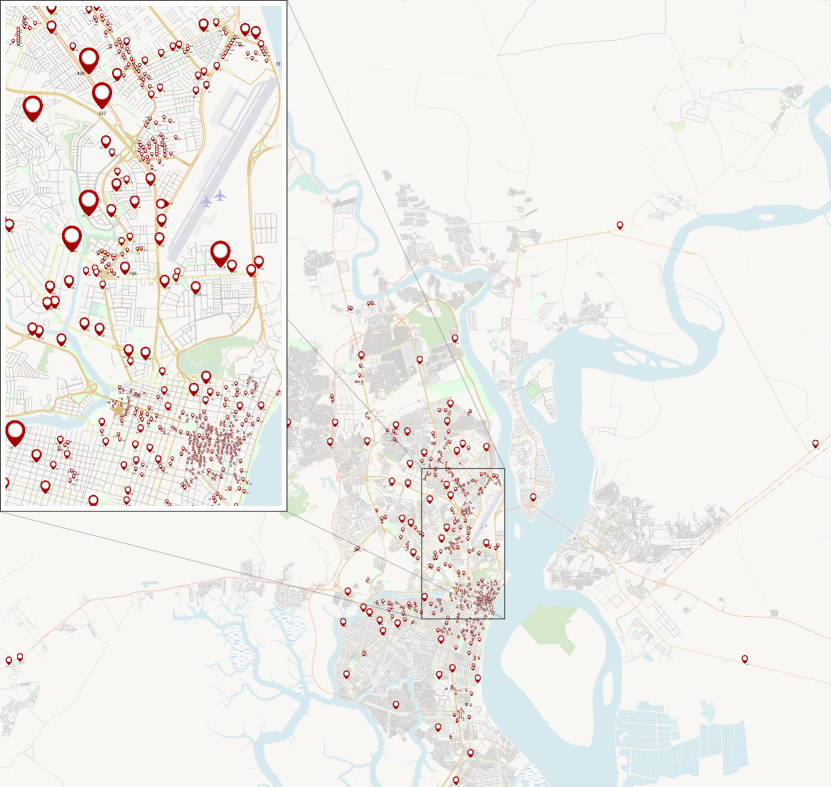
Figure 4: Map of Guayaquil displaying the stores to be visited.

4.3 Results and solution visualization

At a first attempt to solve the IP implementation of IVPRM, for a small number of nodes in the graph ($n=15$), no feasible solution was found even by using an HPC server. A similar result was obtained when attempting to use the variable fixing heuristic. These facts motivated the construction and application of the three-phase solution approach captured by Algorithm 1. The following tables describe the behavior of the latter algorithm using the real-world data. It is important to remark that a lower bound for the number of partitions is considered as the ratio between the total service time and the total working time of the available pollsters per day ($\underline{k}=10$).

Table 5: Statistics of the partitions obtained with Algorithm 1

$\#$ Subsets	$\mathbf{n}_{\textbf{min}}$	$\mathbf{n}_{\textbf{max}}$	Minimum	Maximum	$\#$ Subsets with
$k$			service time	service time	feasible solutions
10	56	100	538.7	570.6	0
12	36	97	446.5	478.1	0
14	16	79	380.7	412.1	0
16	35	65	330.9	362.6	0
18	14	68	292.8	324.0	0
20	11	60	261.6	293.2	1
22	10	57	236.2	268.1	3
24	11	54	215.2	247.0	7
26	10	52	197.5	229.1	6
28	7	43	134.9	214.1	16
30	7	43	153.7	216.4	30

Table 5 contains general information about partitions of the set of vertices of the graph for several values of $k$, which is the number of subsets in each partition. For each $k$ and $N_{\max}=5000$, the minimum number of vertices $n_{\min}$, the maximum number of vertices $n_{\max}$, and the minimum and maximum service times over all subsets in the partition are reported. The last column reports the number of subsets in the partition for which a feasible solution was found by the solver Gurobi in at most $T_{\max}=60$ min. Observe that for $k\in\{10,12,\dots,28\}$, Algorithm 1 can not construct a feasible daily plan since there are not as many solutions as subsets per partition.

In despite of the fact that the maximum available number of pollsters and vehicles at INEC are $|E|=5$ and $|K|=3$, Algorithm 1 always reported that two pollsters and one vehicle are enough to construct every half-shift of a feasible daily plan. Therefore, Table 6 reports the time of the last vehicular arrival at the depot for each subset of the reported partition with $k=30$. For instance, the workload of subset $24$ is made in at most $2$ hours.

Table 6: Solutions for a 30–way partition

Subsets 0 — 9		Subsets 10 — 19		Subsets 20 — 29
	Arrival time		Arrival time		Arrival time
0	1 h 36 min	10	2 h 28 min	20	3 h 03 min
1	1 h 55 min	11	2 h 14 min	21	2 h 01 min
2	2 h 02 min	12	1 h 39 min	22	1 h 43 min
3	1 h 55 min	13	2 h 19 min	23	1 h 45 min
4	2 h 08 min	14	1 h 55 min	24	2 h 00 min
5	1 h 57 min	15	3 h 30 min	25	2 h 08 min
6	2 h 18 min	16	2 h 42 min	26	2 h 18 min
7	1 h 50 min	17	2 h 14 min	27	2 h 18 min
8	2 h 49 min	18	2 h 16 min	28	1 h 47 min
9	3 h 03 min	19	2 h 04 min	29	1 h 54 min

The results of the linking partition step are reported in Table 7. A pair of subsets are assigned to each day $s\in\{0,\ldots,14\}$, which correspond to a morning and afternoon half-shift needed to accomplish the workload. For example, day $11$ synces subsets $27$ and $1$ for a total daily working time of $4$ h $53$ min including a $40$ min break between shifts. The first subset of stores is polled in the morning, and the second is visited in the afternoon. As it can be seen in Table 6, each daily plan is accomplished by $2$ pollsters and $1$ vehicle, concluding the workload in a time horizon of 15 days. The latter result contrasts with the empirical solution provided by INEC in which $5$ pollsters and $3$ vehicles were required in a time horizon of $17$ days. As the daily income of each pollster is $\$40$, and the daily cost of hiring and using a vehicle is $\$100$, the empirical solution currently used by INEC approximately duplicates the cost of the aggregated daily plan found with Algorithm 1.

Table 7: Daily plan results of Algorithm 1

Daily plans 0 — 7				Daily plans 8 — 14
$s$	Synced	Working		$s$	Synced	Working
	subsets	time			subsets	time
0	$15\to 0$	5 h 45 min		8	$20\to 12$	5 h 22 min
1	$9\to 22$	5 h 26 min		9	$8\to 23$	5 h 14 min
2	$16\to 28$	5 h 10 min		10	$10\to 7$	4 h 59 min
3	$13\to 29$	4 h 53 min		11	$\bf 27\to 1$	4 h 53 min
4	$6\to 14$	4 h 54 min		12	$26\to 3$	4 h 53 min
5	$18\to 5$	4 h 53 min		13	$11\to 24$	4 h 55 min
6	$17\to 21$	4 h 56 min		14	$4\to 2$	4 h 51 min
7	$25\to 19$	4 h 52 min			Average:	5 h 03 min

Finally, the resulting real aggregated daily plan presented above is depicted in Figure 5. On the left upper corner, the afternoon shift of the eighth working day, namely subset 12, is zoomed in. There, the stores that are visited by the first and second pollster are represented by circles and squares, respectively. Each store is labeled with a number between 1 and 820. Continuous and dashed lines represent routes; the former for pedestrians and the latter for vehicles.

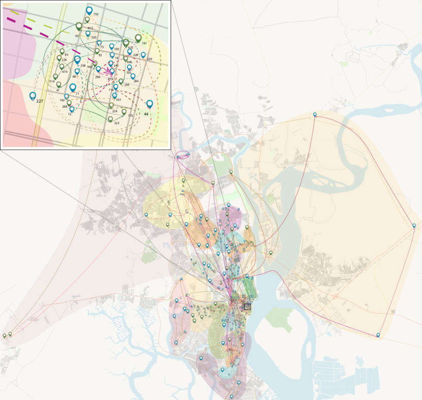
Figure 5: Map of Guayaquil displaying the partition subsets, stores, and routes.

5 Conclusions

The Integrated Vehicle and Pollster Routing Problem (IVPRP), focused on the transportation of pollsters with pedestrian and vehicular routes, has been introduced in this paper. It generalizes of the Pick-up and Delivery Problem combining well-known problems such as the Share-a-Ride, the Integrated Dial-a-Ride, and the periodic VRP with time windows and backhaulings. The complexity of the IVPRP problem has been shown to be $\mathcal{NP}$ – hard by reduction from the Traveling Salesman Problem.

A mixed integer formulation was proposed for this problem, and it was assesed using real-world data. Due to the hardness of the problem, a three-phase heuristic method was devised: the set of stores to be visited is partitioned at the first stage, then pollsters and vehicles are routed on each subset, and finally pairs of subsets are linked as half-shifts of an aggregated daily plan.

The algorithm was tested with a real-world instance at Guayaquil, the second most important city of Ecuador. The data was provided by INEC with information related to 820 stores to be visited monthly. The heuristically-found solution improved the one designed by INEC reducing approximately two times the operational costs, since half of the available workforce and fleet are required. Moreover, the resulting aggregated daily plan takes two days less than the former empirical solution. Despite the computational intractability of this problem, the previous results can be improved by working on tighter formulations and exact algorithms, which are interesting topics for future research.

References

- Alvarenga and Mateus [2004] G. B. Alvarenga and G. R. Mateus. A two-phase genetic and set partitioning approach for the vehicle routing problem with time windows. In Fourth International Conference on Hybrid Intelligent Systems (HIS’04), pages 428–433, 2004.
- Baldacci et al. [2007] Roberto Baldacci, Nicos Christofides, and Aristide Mingozzi. An exact algorithm for the vehicle routing problem based on the set partitioning formulation with additional cuts. Mathematical Programming, 115(2):351–385, August 2007. doi: 10.1007/s10107-007-0178-5.
- Battarra et al. [2014] Maria Battarra, Jean-François Cordeau, and Manuel Iori. Pickup-and-Delivery Problems for Goods Transportation, pages 161 – 191. Society for Industrial and Applied Mathematics, Philadelphia, PA, 2 edition, 2014. doi: 10.1137/1.9781611973594.
- Boeing [2017] Geoff Boeing. OSMnx: New methods for acquiring, constructing, analyzing, and visualizing complex street networks. Computers, Environment and Urban Systems, 65:126–139, sep 2017. doi: 10.1016/j.compenvurbsys.2017.05.004.
- Borndörfer et al. [1999] R. Borndörfer, M. Grötschel, F. Klostermeier, and C. Küttner. Telebus berlin: Vehicle scheduling in a dial-a-ride system. In Lecture Notes in Economics and Mathematical Systems, pages 391–422. Springer Berlin Heidelberg, 1999. doi: 10.1007/978-3-642-85970-0˙19.
- Braekers et al. [2014] Kris Braekers, An Caris, and Gerrit K. Janssens. Exact and meta-heuristic approach for a general heterogeneous dial-a-ride problem with multiple depots. Transportation Research Part B: Methodological, 67:166–186, September 2014. doi: 10.1016/j.trb.2014.05.007.
- Chowmali and Sukto [2020] Wasana Chowmali and Seekharin Sukto. A novel two-phase approach for solving the multi-compartment vehicle routing problem with a heterogeneous fleet of vehicles: a case study on fuel delivery. Decision Science Letters, pages 77–90, 2020. doi: 10.5267/j.dsl.2019.7.003.
- Christofides et al. [1981] N. Christofides, A. Mingozzi, and P. Toth. Exact algorithms for the vehicle routing problem, based on spanning tree and shortest path relaxations. Mathematical Programming, 20(1):255–282, December 1981. doi: 10.1007/bf01589353.
- Clarke and Wright [1964] G. Clarke and J. W. Wright. Scheduling of vehicles from a central depot to a number of delivery points. Operations Research, 12(4):568–581, August 1964. doi: 10.1287/opre.12.4.568.
- Cordeau et al. [2005] Jean-François Cordeau, Michel Gendreau, Alain Hertz, Gilbert Laporte, and Jean-Sylvain Sormany. New heuristics for the vehicle routing problem. In Logistics Systems: Design and Optimization, pages 279–297. Springer-Verlag, 2005. doi: 10.1007/0-387-24977-x˙9.
- Cordeau and Laporte [2003] Jean-Franois Cordeau and Gilbert Laporte. The dial-a-ride problem (DARP): Variants, modeling issues and algorithms. Quarterly Journal of the Belgian, French and Italian Operations Research Societies, 1(2), June 2003. doi: 10.1007/s10288-002-0009-8.
- Coslovich et al. [2006] Luca Coslovich, Raffaele Pesenti, and Walter Ukovich. A two-phase insertion technique of unexpected customers for a dynamic dial-a-ride problem. European Journal of Operational Research, 175(3):1605–1615, December 2006. doi: 10.1016/j.ejor.2005.02.038.
- Dantzig and Ramser [1959] G. B. Dantzig and J. H. Ramser. The truck dispatching problem. Management Science, 6(1):80–91, October 1959.
- Doerner and Salazar-González [2014] Karl F. Doerner and Juan-José Salazar-González. Pickup-and-Delivery Problems for People Transportation, pages 193 – 212. Society for Industrial and Applied Mathematics, Philadelphia, PA, 2 edition, 2014. doi: 10.1137/1.9781611973594.
- Drexl et al. [2013] Michael Drexl, Julia Rieck, Thomas Sigl, and Bettina Press. Simultaneous vehicle and crew routing and scheduling for partial- and full-load long-distance road transport. Business Research, 6(2):242–264, November 2013. doi: 10.1007/bf03342751.
- Ferrucci [2013] Francesco Ferrucci. Pro-active Dynamic Vehicle Routing. Springer Berlin Heidelberg, 2013. ISBN 978-3-642-33472-6. doi: 10.1007/978-3-642-33472-6.
- Fikar and Hirsch [2015] Christian Fikar and Patrick Hirsch. A matheuristic for routing real-world home service transport systems facilitating walking. Journal of Cleaner Production, 105:300–310, October 2015. doi: 10.1016/j.jclepro.2014.07.013.
- Florio et al. [2020] Alexandre M. Florio, Richard F. Hartl, and Stefan Minner. New exact algorithm for the vehicle routing problem with stochastic demands. Transportation Science, 54(4):1073–1090, July 2020. doi: 10.1287/trsc.2020.0976.
- Furtado et al. [2017] Maria Gabriela S. Furtado, Pedro Munari, and Reinaldo Morabito. Pickup and delivery problem with time windows: A new compact two-index formulation. Operations Research Letters, 45(4):334–341, July 2017. doi: 10.1016/j.orl.2017.04.013.
- Gendreau et al. [1994] Michel Gendreau, Alain Hertz, and Gilbert Laporte. A tabu search heuristic for the vehicle routing problem. Management Science, 40(10):1276–1290, October 1994. doi: 10.1287/mnsc.40.10.1276.
- Gracia et al. [2014] Carlos Gracia, Borja Velázquez-Martí, and Javier Estornell. An application of the vehicle routing problem to biomass transportation. Biosystems Engineering, 124:40–52, August 2014. doi: 10.1016/j.biosystemseng.2014.06.009.
- Ho et al. [2018] Sin C. Ho, W.Y. Szeto, Yong-Hong Kuo, Janny M.Y. Leung, Matthew Petering, and Terence W.H. Tou. A survey of dial-a-ride problems: Literature review and recent developments. Transportation Research Part B: Methodological, 111:395–421, May 2018. doi: 10.1016/j.trb.2018.02.001.
- Kaibel et al. [2011] Volker Kaibel, Matthias Peinhardt, and Marc E. Pfetsch. Orbitopal fixing. Discrete Optimization, 8(4):595–610, nov 2011. doi: 10.1016/j.disopt.2011.07.001.
- Lam et al. [2020] Edward Lam, Pascal Van Hentenryck, and Phil Kilby. Joint vehicle and crew routing and scheduling. Transportation Science, 54(2):488–511, March 2020. doi: 10.1287/trsc.2019.0907.
- Laporte et al. [1984] Gilbert Laporte, Martin Desrochers, and Yves Nobert. Two exact algorithms for the distance-constrained vehicle routing problem. Networks, 14(1):161–172, 1984. doi: 10.1002/net.3230140113.
- Linfati et al. [2018] Rodrigo Linfati, John Willmer Escobar, and Juan Escalona. A two-phase heuristic algorithm for the problem of scheduling and vehicle routing for delivery of medication to patients. Mathematical Problems in Engineering, 2018:1–12, December 2018. doi: 10.1155/2018/8901873.
- Madsen et al. [1995] Oli B. G. Madsen, Hans F. Ravn, and Jens Moberg Rygaard. A heuristic algorithm for a dial-a-ride problem with time windows, multiple capacities, and multiple objectives. Annals of Operations Research, 60(1):193–208, December 1995. doi: 10.1007/bf02031946.
- Margot [2009] François Margot. Symmetry in Integer Linear Programming. In 50 Years of Integer Programming 1958-2008, pages 647–686. Springer Berlin Heidelberg, nov 2009. doi: 10.1007/978-3-540-68279-0˙17.
- Masson et al. [2014] Renaud Masson, Fabien Lehuédé, and Olivier Péton. The dial-a-ride problem with transfers. Computers & Operations Research, 41:12–23, January 2014. doi: 10.1016/j.cor.2013.07.020.
- Melachrinoudis et al. [2007] Emanuel Melachrinoudis, Ahmet B. Ilhan, and Hokey Min. A dial-a-ride problem for client transportation in a health-care organization. Computers & Operations Research, 34(3):742–759, March 2007. doi: 10.1016/j.cor.2005.03.024.
- Molenbruch et al. [2017] Yves Molenbruch, Kris Braekers, and An Caris. Typology and literature review for dial-a-ride problems. Annals of Operations Research, 259(1-2):295–325, May 2017. doi: 10.1007/s10479-017-2525-0.
- Molenbruch et al. [2021] Yves Molenbruch, Kris Braekers, Patrick Hirsch, and Marco Oberscheider. Analyzing the benefits of an integrated mobility system using a matheuristic routing algorithm. European Journal of Operational Research, 290(1):81–98, April 2021. doi: 10.1016/j.ejor.2020.07.060.
- Osman [1993] Ibrahim Hassan Osman. Metastrategy simulated annealing and tabu search algorithms for the vehicle routing problem. Annals of Operations Research, 41(4):421–451, December 1993. doi: 10.1007/bf02023004.
- Ostrowski et al. [2009] James Ostrowski, Jeff Linderoth, Fabrizio Rossi, and Stefano Smriglio. Orbital branching. Mathematical Programming, 126(1):147–178, mar 2009. doi: 10.1007/s10107-009-0273-x.
- Parragh et al. [2008a] Sophie N. Parragh, Karl F. Doerner, and Richard F. Hartl. A survey on pickup and delivery problems. Journal für Betriebswirtschaft, 58(2):81–117, May 2008a. doi: 10.1007/s11301-008-0036-4.
- Parragh et al. [2008b] Sophie N. Parragh, Karl F. Doerner, and Richard F. Hartl. A survey on pickup and delivery problems. Part I: Transportation between customers and depot. Journal für Betriebswirtschaft, 58(1):21 – 51, 2008b. ISSN 1614-631X. doi: 10.1007/s11301-008-0033-7.
- Parragh et al. [2008c] Sophie N. Parragh, Karl F. Doerner, and Richard F. Hartl. A survey on pickup and delivery problems. Part II: Transportation between pickup and delivery locations. Journal für Betriebswirtschaft, 58(2):81 – 117, 2008c. ISSN 1614-631X. doi: 10.1007/s11301-008-0036-4.
- Pisinger and Ropke [2007] David Pisinger and Stefan Ropke. A general heuristic for vehicle routing problems. Computers & Operations Research, 34(8):2403–2435, August 2007. doi: 10.1016/j.cor.2005.09.012.
- Recalde et al. [2018] Diego Recalde, Daniel Severín, Ramiro Torres, and Polo Vaca. An exact approach for the balanced -way partitioning problem with weight constraints and its application to sports team realignment. Journal of Combinatorial Optimization, 36(3):916–936, feb 2018. doi: 10.1007/s10878-018-0254-1.
- Sartori and Buriol [2018] Carlo S. Sartori and Luciana S. Buriol. A Matheuristic Approach to the Pickup and Delivery Problem with Time Windows. In Lecture Notes in Computer Science, pages 253–267. Springer International Publishing, 2018. doi: 10.1007/978-3-030-00898-7˙16.
- Savelsbergh and Sol [1995] M. W. P. Savelsbergh and M. Sol. The general pickup and delivery problem. Transportation Science, 29(1):17–29, February 1995. doi: 10.1287/trsc.29.1.17.
- Taillard [1993] É. Taillard. Parallel iterative search methods for vehicle routing problems. Networks, 23(8):661–673, December 1993. doi: 10.1002/net.3230230804.
- Toffolo et al. [2019] Túlio A.M. Toffolo, Thibaut Vidal, and Tony Wauters. Heuristics for vehicle routing problems: Sequence or set optimization? Computers & Operations Research, 105:118–131, May 2019. doi: 10.1016/j.cor.2018.12.023.
- Vidal et al. [2013] Thibaut Vidal, Teodor Gabriel Crainic, Michel Gendreau, and Christian Prins. Heuristics for multi-attribute vehicle routing problems: A survey and synthesis. European Journal of Operational Research, 231(1):1–21, November 2013. doi: 10.1016/j.ejor.2013.02.053.