Nonlocal network dynamics via fractional graph Laplacians

Abstract

We introduce nonlocal dynamics on directed networks through the construction of a fractional version of a nonsymmetric Laplacian for weighted directed graphs. Furthermore, we provide an analytic treatment of fractional dynamics for both directed and undirected graphs, showing the possibility of exploring the network employing random walks with jumps of arbitrary length. We also provide some examples of the applicability of the proposed dynamics, including consensus over multi-agent systems described by directed networks. network dynamics, nonlocal dynamics, superdiffusion, matrix functions, power law decay
2010 Math Subject Classification: 91D30, 60J20, 94C15

1 Introduction

Systems made of highly interconnected units, where the connection stands for a kind of (possibly one-directional) interaction between the different nodes, are a ubiquitous modeling approach for several natural and man-made phenomena. Examples include social interactions in the real and digital world, gene regulatory networks, networks of chemical reactions, phone call networks, and many others. An efficient way for representing these complex interactions is through the use of graphs models. One of the main goals in this framework is to develop techniques and measures that are capable to characterize the topology of real networks, i.e., of graphs whose structure is irregular, complex and, possibly, evolving in time. A highly successful approach is to explore the network structure by means of random walks and other diffusive-type processes defined on the underlying graph.

Here we investigate the behavior of certain nonlocal dynamical processes evolving on the network. In these models, a random walker on the network is not constrained to hop only from one node to adjacent nodes, but is allowed to perform long distance jumps, albeit with a lower probability. One can also phrase these processes as anomalous diffusion phenomena, or superdiffusion.

Recently, two main approaches have been proposed to construct such nonlocal dynamics on graphs. The first one can be expressed in terms of multi hopper exploration strategies on the network [11, 12, 13], leading to a probability distribution that permits the hopper to (occasionally) perform long distance jumps. Such long range transitions, often referred to as Lévy flights, can also be described in the framework of the fractional calculus [25]. Recent papers investigated some aspects of this phenomenon (in terms of anomalous diffusion) in the case of undirected graphs, making use of the (symmetric) fractional graph Laplacian and its normalized version; see [28].

The present paper has two main goals. One of them is to extend the notion of nonlocal dynamics to directed networks, investigating how the network structure affects the properties of a dynamical system evolving on it while accounting for the orientation of the connections. Similar to the approach in [28], the method we propose can be formulated as the problem of evolving a system of ordinary differential equations in time using as coefficient matrix the fractional powers of a Laplacian of the underlying graph; an important difference, however, is that in the directed case the Laplacian matrix is nonsymmetric, hence the definition of fractional powers is more delicate than in the undirected (symmetric) case. This is done in Section 2. Our second goal is related to the work presented in in [28] and consists in a rigorous analysis of the decay behavior in the entries of the $\alpha$th power of the Laplacian matrix and its exponential. As we will see, in the undirected case (symmetric Laplacian) we can obtain very general results, applicable to virtually any network. To complement the analysis, we show also that the fractional Laplacian of some simple infinite graphs induces a stable probability distribution with superdiffusive properties. Specifically, in Section 3 we explore the decay properties of the transition probabilities of nonlocal random walks induced by the fractional Laplacian of undirected networks, and we offer some remarks on their possible extension to the directed case. Subsequently, in Section 4 we analyze the superdiffusive behavior of the proposed dynamic on some simple infinite graphs (both directed and undirected), proving that it appears naturally as a stationary distribution for both the undirected and directed case by exploiting the techniques used in [12] for the $k$–path Laplacian; see Section 5. In the directed case, the dynamics exhibit some similarities but also interesting differences with respect to to the undirected case. Finally, we consider two applications to real world directed networks in Section 6.

1.1 Preliminaries and notation on graphs

We recall here some basic notions on graphs that will be used in the following discussions. A directed graph, or digraph, is a pair $G=(V,E)$, where $V=\{v_{1},\ldots,v_{n}\}$ is a set of nodes (or vertices), and $E~{}\subseteq~{}V\times V$ is a set of ordered pairs of nodes called edges. We define on $V$ the binary relation $v_{i}\sim v_{j}$ if $(v_{i},v_{j})\in E$, or $(v_{j},v_{i})\in E$. A weighted directed graph $G~{}=~{}(V,E,W)$ is then obtained by considering a weight matrix $W$ with nonnegative entries $(W)_{i,j}=w_{i,j}\geq 0$ and such that $w_{i,j}>0$ if and only if $(v_{i},v_{j})$ is an edge of $G$. If all the nonzero weights have value $1$ we omit the weighted specification. For every node $v\in V$, the degree $\deg(v)$ of $v$ is the number of edges leaving or entering $v$ taking into account their weights,

$$d_{i}=\deg(v_{i})=\sum_{j\,:\,{v_{i}\sim v_{j}}}w_{i,j}.$$ (1)

A vertex is isolated if its degree is zero.

The degree matrix $D$ is then the diagonal matrix whose entries are given by the degrees of the nodes, i.e.,

$$\begin{split}D=&\operatorname{diag}(\deg(v_{1}),\ldots,\deg(v_{n}))=\operatorname{diag}(d_{1},\ldots,d_{n}).\end{split}$$ (2)

In light of the fact that we want to consider dynamical processes on directed graphs, it is useful to separate the degrees also between the incoming and outgoing edges with respect to the node $v_{i}$, i.e., to consider the in–degrees and out–degrees

$$d_{i}^{(\text{in})}=\operatorname{\deg_{\text{in}}}(v_{i})=\sum_{j\,:\,(v_{j},v_{i})\in E}w_{j,i},\qquad d_{i}^{(\text{out})}=\operatorname{\deg_{\text{out}}}(v_{i})=\sum_{j\,:\,(v_{i},v_{j})\in E}w_{i,j},$$

together with the related diagonal matrices $D_{\text{in}}=\operatorname{diag}(\operatorname{\deg_{\text{in}}}(v_{1}),\ldots,\operatorname{\deg_{\text{in}}}(v_{n}))=\operatorname{diag}(d^{(\text{in})}_{1},\ldots,d^{(\text{in})}_{n})$, and $D_{\text{out}}=\operatorname{diag}(\operatorname{\deg_{\text{out}}}(v_{1}),\ldots,\operatorname{\deg_{\text{out}}}(v_{n}))=\operatorname{diag}(d^{(\text{out})}_{1},\ldots,d^{(\text{out})}_{n})$. Moreover, we assume from now on that no vertex of the graph is isolated, and that all the graphs are loop-less, i.e., that there is no edge going from a vertex to itself. Given a weighted directed graph $G=(V,E,W)$ with $V=\{v_{1},\ldots,v_{n}\}$ and $E=\{e_{1},\ldots,e_{m}\}$, the incidence matrix $B$ of $G$ is the $n\times m$ matrix whose entries $b_{i,j}$ are given by

$$b_{i,j}=\left\{\begin{array}[]{ll}{+\sqrt{w_{i,k}}},&\text{ if }e_{j}=(v_{i},v_{k})\text{ for some }k,\\ {-\sqrt{w_{k,i}}},&\text{ if }e_{j}=(v_{k},v_{i})\text{ for some }k,\\ 0,&\text{ otherwise.}\end{array}{}\right.$$ (3)

Observe that the choice of the sign in $B$ is purely conventional.

If the ordering of the vertices in the edges in $E$ is not relevant, i.e., if each edge can be traversed both ways, we move from directed graphs to undirected graphs; that is, an undirected graph is a pair $G=(V,E)$, where $V=\{v_{1},\ldots,v_{n}\}$ is a set of nodes or vertices, and $E\subseteq V\times V$ is a set of edges such that if $(v_{i},v_{j})\in E$, then $(v_{j},v_{i})\in E$ for all $i,j$. A weighted undirected graph $G=(V,E,W)$ is then obtained by considering a (symmetric) weight matrix $W$ with nonnegative entries $(W)_{i,j}=w_{i,j}\geq 0$ and such that $w_{i,j}>0$ if and only if $(v_{i},v_{j})$ is an edge of $G$. If all the nonzero weights have value $1$ we omit the weighted specification. For any two nodes $u,v\in V$ in a graph $G=(V,E)$, a walk from $u$ to $v$ is an ordered sequence of nodes $(v_{0},v_{1},\ldots,v_{k})$ such that $v_{0}=u$, $v_{k}=v$, and $(v_{i},v_{i+1})\in E$ for all $i=0,\ldots,k-1$. The integer $k$ is the length of the walk. The walk is closed if the initial and terminal nodes coincide, i.e., $u=v$. A cycle in a graph is a nonempty closed walk in which the only repeated vertices are the first and last. An undirected graph $G$ is connected if for any two distinct nodes $u,v\in V$, there is a walk between $u$ and $v$. A directed graph $G$ is strongly connected if for any two distinct nodes $u,v\in V$, there is a directed walk from $u$ to $v$. For both a directed and an undirected graph $G$ we introduce the adjacency matrix $A$ as the $n\times n$ matrix with elements

$$(A)_{i,j}=a_{i,j}=\left\{\begin{array}[]{cc}1,&\text{ if }(v_{i},v_{j})\in E,\\ 0,&\text{ otherwise}.\end{array}\right.$$

Observe that the adjacency matrix $A$ of an undirected graph $G$ is always symmetric. In particular, if $G=(V,E)$ is a graph, given two nodes $u,v\in V$, we say that $u$ is adjacent to $v$ and write $u\sim v$, if $(u,v)\in E$. The above binary relation is symmetric if $G$ is an undirected graph, while in general it is not for a directed graph. Note that for an unweighted graph, $W=A$.

1.1.1 Graph Laplacian

Next, we recall the definition of the Laplacian matrix for an undirected graph and then discuss an extension of it we will use in the case of directed graphs.

Definition 1.1 (Graph Laplacian).

Let $G=(V,E)$ be a weighted undirected graph with weight matrix $W$, weighted degree matrix $D$ and weighted incidence matrix $B$. Then the graph Laplacian $L$ of $G$ is

$$L=D-W=BB^{T}.$$

The normalized random walk version of the graph Laplacian is

$$D^{-1}L=I-D^{-1}W=D^{-1}BB^{T},$$

where $I$ is the identity matrix. Observe that $D^{-1}W$ is a row–stochastic matrix, i.e. it is nonnegative with row sums equal to 1. The normalized symmetric version is

$$D^{-\frac{1}{2}}LD^{-\frac{1}{2}}=I-D^{-\frac{1}{2}}WD^{-\frac{1}{2}}.$$

If $G$ is unweighted then $W=A$ in the above definitions. Here we assume that every vertex has nonzero degree.

In the case of a directed graph the situation is more intricate since many nonequivalent definitions of the Laplacian exist. We can easily define, mimicking Definition 1.1, the nonnormalized version with respect to the in– and out–degrees, in both the weighted and unweighted case.

Definition 1.2 (Directed graph Laplacian).

Let $G=(V,E,W)$ be a weighted directed graph, with degree matrices $D_{\text{out}}$ and $D_{\text{in}}$ The nonnormalized directed graph Laplacian $L_{\text{out}}$ and $L_{\text{in}}$ of $G$ are

$$L_{\text{out}}=D_{\text{out}}-W,\qquad L_{\text{in}}=D_{\text{in}}-W.$$

To define the normalized versions, we need to invert either the $D_{\text{in}}$ or the $D_{\text{out}}$ matrices, but the absence of isolated vertices is no longer sufficient to ensure this, since there could be a node with only outgoing or ingoing edges. A first way of overcoming this issue could be to impose that every vertex has at least one outgoing and one incoming edges, which is rather restrictive. Otherwise, we could restrict our attention to the set of nodes having an out–degree or in–degree different from zero, as in [2]. Another approach, that avoids reducing the size of the graph, is instead to mimic the recipe for the PageRank algorithm [26] and replace any diagonal zeros in $D_{\text{in}}$, respectively $D_{\text{out}}$, with ones, while replacing the corresponding (zero) column, respectively row, of $W$ with the vector with entries $1/n$.

The last approach we briefly mention is the one presented in [8]. In this case a symmetric Laplacian is constructed also for a directed graph. However, it is easy to see that this kind of approach may return the same Laplacian matrix for nonisomorphic graphs. This also happens if we define a symmetric digraph Laplacian by using the incidence matrix $B$ of Definition 3 and construct $L=BB^{T}$ as in Definition 1.1. In the rest of the paper we focus mainly on the nonsymmetric Laplacian $L_{\text{out}}$ and its normalized version.

2 Fractional Laplacians of a directed graph

To justify the use of a fractional Laplacian for exploring the structure of the network, let us first consider a simple diffusion problem in the case in which $G$ is an undirected graph. Let $u:V\rightarrow\mathbb{R}$ describe a “heat” distribution on the nodes of the graph with heat diffusivity $\kappa$. We can express the variation of heat in the nodes as

$$\begin{split}\displaystyle\frac{\text{d}}{\text{d}t}u(t)=&-\kappa\sum_{j\,:\,(v_{j},v_{i})\in E}(u_{i}-u_{j})=-\kappa\left(u_{i}\sum_{j\,:\,(v_{j},v_{i})\in E}1-\sum_{j\,:\,(v_{j},v_{i})\in E}u_{j}\right)\\ =&-\kappa\left(u_{i}\deg(v_{i})-\sum_{j\,:\,(v_{j},v_{i})\in E}u_{j}\right)=-\kappa\sum_{j\,:\,(v_{j},v_{i})\in E}\left(\delta_{i,j}\deg(v_{i})-1\right)u_{j}\\ =&-\kappa\sum_{j\,:\,(v_{j},v_{i})\in E}(L)_{i,j}u_{j},\end{split}$$

which in matrix form reads

$$\begin{split}\text{find }u\,:&\,[0,T]\longrightarrow\mathbb{R}^{n}\\ \text{ s.t. }&\left\{\begin{array}[]{ll}\displaystyle\frac{\text{d}}{\text{d}t}u(t)=-\kappa Lu(t),&t\in(0,T],\\ u(0)=u_{0},&\text{prescribed,}\end{array}\right.\end{split}$$ (4)

where now $L$ is the unweighted Laplacian from Definition 1.1. Since $L$ is a symmetric positive semidefinite matrix, one can apply the process of “fractionalization” considered in [18, 19] for the continuous Laplace operator. Consider the spectral decomposition of the Laplacian matrix,

$$L=U\Lambda U^{T},\qquad U^{T}U=I,\qquad\Lambda=\operatorname{diag}(\lambda_{1},\dots,\lambda_{n}).$$

Following [28], we define the fractional graph Laplacian as

$$\begin{split}&L^{\alpha}=U\Lambda^{\alpha}U^{T},\qquad U^{T}U=I,\\ &\Lambda^{\alpha}=\operatorname{diag}(\lambda_{1}^{\alpha},\ldots,\lambda_{n}^{\alpha}),\qquad\alpha\in(0,1].\end{split}$$ (5)

Note that the fractional powers $\lambda_{1}^{\alpha},\dots,\lambda_{n}^{\alpha}$ are well defined because the eigenvalues of the Laplacian matrix are nonnegative. This follows from the fact that the Laplacian is an $M$-matrix, see Definition 2.3.

The definition of the fractional graph Laplacian becomes significantly different when the case of the (nonnormalized) digraph Laplacian from Definition 1.2 is considered. In general, this operator is non normal, and thus we cannot define the fractional power as in (5). Therefore, we need to define the $\alpha$th power of a non normal matrix.

Without loss of generality, we focus the analysis on the out–degree Laplacian $L_{\text{out}}=D_{\text{out}}-A$ since it remains essentially the same in the case of the in–degree Laplacian. We first recall a suitable definition for the matrix function $f(A)$ for a generic matrix $A$, that extends the one based on the diagonalization in (5). This definition can be stated in terms of the Jordan canonical form of the matrix [16, Section 1.2.2].

We recall that any matrix $A\in\mathbb{C}^{n\times n}$ can be expressed in Jordan canonical form as

$$Z^{-1}AZ=J=\operatorname{diag}(J_{1},\ldots,J_{p}),\quad\text{ for }J_{k}=J_{k}(\lambda_{k})=\begin{bmatrix}\lambda_{k}&1\\ &\lambda_{k}&\ddots\\ &&\ddots&1\\ &&&\lambda_{k}\end{bmatrix}\in\mathbb{C}^{m_{k}\times m_{k}},$$ (6)

where $Z$ is nonsingular and $m_{1}+m_{2}+\ldots+m_{p}=n$. If each block in which the eigenvalue $\lambda_{k}$ appears is of size 1 then $\lambda_{k}$ is said to be a semisimple eigenvalue.

Let us denote by $\lambda_{1},\ldots,\lambda_{s}$ the distinct eigenvalues of $A$, and by $n_{i}$ the order of the largest Jordan block in which the $\lambda_{i}$ appears, i.e., the index of the eigenvalue $\lambda_{i}$. We have the following definition.

Definition 2.1.

The function $f$ is defined on the spectrum of $A$ if the values

$$f^{(j)}(\lambda_{i}),\qquad j=0,1,\ldots,n_{i}-1,\quad i=1,\ldots s,$$

exist, where $f^{(j)}$ denotes the $j$th derivative of $f$, with $f^{(0)}=f$.

We can define the matrix function $f(A)$ for a generic matrix $A$ by using the Jordan canonical form, provided that the function $f$ is defined on the spectrum of $A$.

Definition 2.2.

Lef $f$ be defined on the spectrum of $A\in\mathbb{C}^{n\times n}$, which is represented in Jordan canonical form as in (6). Then,

$$f(A)=Zf(J)Z^{-1}=Z\operatorname{diag}(f(J_{1}),\ldots,f(J_{p}))Z^{-1},$$

where

$$f(J_{k})=\begin{bmatrix}f(\lambda_{k})&f^{\prime}(\lambda_{k})&\ldots&\frac{f^{(m_{k}-1)}(\lambda_{k})}{(m_{k}-1)!}\\ &f(\lambda_{k})&\ddots&\vdots\\ &&\ddots&f^{\prime}(\lambda_{k})\\ &&&f(\lambda_{k})\end{bmatrix}.$$

Moreover, let $f$ be a multivalued function and suppose some eigenvalues occur in more than one Jordan block. If the same choice of branch of $f$ is made in each block, then we say that $f(A)$ is a primary matrix function. In this paper we only consider primary matrix functions.

Note that in the real symmetric case, given in (5), the Jordan canonical form reduces to the diagonalization of the matrix.

In order to ensure that $f(L_{\text{out}})=L_{\text{out}}^{\alpha}$, $\alpha\in(0,1]$ is well defined, we need to check first that $f(x)=x^{\alpha}$ is defined on the spectrum of $L_{\text{out}}$ (Definition 2.1). In the following discussion, by $f(x)=x^{\alpha}$ we refer to the branch with a cut on the negative real line, i.e. if $x=\rho e^{i\theta}$ with $\rho>0$ and $\theta\in(-\pi,\pi)$, then $x^{\alpha}=\rho^{\alpha}e^{i\alpha\theta}$.

This function is defined on the spectrum of the Laplacian because, as in the symmetric case, the matrix $L_{\text{out}}$ is a singular $M$-matrix, with $0$ as a semisimple eigenvalue.

Definition 2.3 ($M$-matrix, [6]).

A matrix $A\in\mathbb{R}^{n\times n}$ is an $M$-matrix if $A=sI-B$ for some nonnegative matrix $B$, where $s\geq\rho(B)$, the spectral radius of $B$. It is a singular $M$-matrix if $s=\rho(B)$.

Note that the real part of a nonzero eigenvalue of a singular $M$-matrix is positive, and that the $M$-matrices form a closed subset $\mathcal{M}$ of the vector space of real matrices $\mathbb{M}_{n}$; we refer to [6] for further information regarding these matrices, including the following basic result, where we denote by $\bm{0}$ the vector of all zeros and by $\bm{1}$ the vector of all ones.

Proposition 2.4 (Properties of $L_{\text{out}}$).

• $L_{\text{out}}$ is a singular $M$-matrix,

• $L_{\text{out}}\bm{1}=\bm{0}$,

• $0$ is a semisimple eigenvalue of $L_{\text{out}}$.

As a consequence we have the following Theorem.

Theorem 2.5.

Given a weighted graph $G=(V,E,W)$ and its Laplacian with respect to the out degree $L_{\text{out}}$ (Definition 1.2), the function $f(x)=x^{\alpha}$ is defined on the spectrum of $L_{\text{out}}$ and induces a matrix function for all $\alpha\in(0,1]$.

Proof 2.6 (Proof of Theorem 2.5).

By Proposition 2.4 we know that $0$ is a semisimple eigenvalue of $L_{\text{out}}$, then all the Jordan blocks related to the eigenvalue $\lambda_{1}=0$ have size 1 and $f(\lambda_{1})=f(0)$ exists. Since $L_{\text{out}}$ is a singular $M$-matrix, $\operatorname{Re}(\lambda_{k})>0$, for all $\lambda_{k}\neq 0$, and $f^{(j)}(\lambda_{k})$ exist for all $j$. Thus, by Definition 2.2, $f$ is defined on the spectrum of $L_{\text{out}}$. Moreover, let $\lambda$ be any nonzero eigenvalue of $L_{\text{out}}$. Then, $\lambda=\rho e^{i\theta}$ with $\theta\in(-\frac{\pi}{2},\frac{\pi}{2})$ since $\operatorname{Re}(\lambda_{k})>0$ and thus we can define $\lambda^{\alpha}=\rho^{\alpha}e^{i\alpha\theta}$ with $\alpha\theta\in(-\frac{\pi}{2},\frac{\pi}{2})$. Therefore, we can always select the branch of $x^{\alpha}$ preserving the positivity of the real part of the eigenvalues, thus ensuring the choice of a primary matrix function.

Under the same hypothesis of Theorem 2.5 we can say more about the structure of $L_{\text{out}}^{\alpha}$. Indeed, this is a result that is already known for the special case of the matrix $p$th root.

Theorem 2.7 ([15]).

If $A$ is a singular $M$-matrix with 0 as a semisimple eigenvalue, then there exists a determination of $A^{1/p}$ for every $p\in\mathbb{N}$ that is a singular $M$-matrix.

Similarly, we get the following useful result.

Theorem 2.8.

If $A$ is a singular $M$-matrix with 0 as a semisimple eigenvalue, then there exists a determination of $A^{\alpha}$ for every $\alpha\in(0,1]$ that is a singular $M$-matrix.

Proof 2.9 (Proof of Theorem 2.8).

Let $A(\varepsilon)=A+\varepsilon I$, then $A(\varepsilon)$ is a nonsingular M–matrix and so is $A(\varepsilon)^{\alpha}$ [14, Corollary 3.7]. By looking at the Jordan canonical forms of the matrices $A(\varepsilon)^{\alpha}$ and $A^{\alpha}$ (Theorem 2.5), we get $A(\varepsilon)^{\alpha}\rightarrow A^{\alpha}$ for $\varepsilon\rightarrow 0$. Clearly, $A^{\alpha}$ is singular, and since the $M$-matrices from a closed subset of $\mathbb{M}_{n}$, we conclude that $A^{\alpha}$ is a singular $M$-matrix.

Moreover, note that the matrix produced in this way is a primary matrix function since we selected the same branch of the $f(x)=x^{\alpha}$ for every matrix of the sequence.

3 Decay bounds for the entries of fractional Laplacians

Quantitative estimates for the entries of fractional powers of the graph Laplacian yield valuable information on the transition probabilities of various types of random walks on the underlying graph. In this section we show how to obtain useful bounds for these quantities using general results on functions of matrices, at least in the case of undirected networks. We also comment on the difficulties one encounters when trying to extend such results to the case of directed graphs.

3.1 Undirected networks

First of all, we show that the fractional Laplacian $L^{\alpha}$ is related to a row–stochastic matrix, which can be used to define a fractional random walk on the graph, similarly to the Laplacian $L$ (see Definition 1.1).

Lemma 3.1.

For $\alpha\in(0,1)$, the matrix

$$P^{(\alpha)}=I-\bar{L}^{(\alpha)},\qquad\text{where }\bar{L}^{(\alpha)}=\operatorname{diag}(L^{\alpha})^{-1}L^{\alpha},$$

is a row–stochastic matrix.

Proof 3.2.

We start by noting that all the diagonal entries of $L^{\alpha}$ are positive, so we have $\operatorname{diag}(\bar{L}^{(\alpha)})=I$ and thus the diagonal entries of $P^{(\alpha)}$ are zero. This can be seen by explicitly writing the eigendecomposition of $L$ and $L^{\alpha}$.

Given that $L\bm{1}=\bm{0}$, we also have $\bar{L}^{(\alpha)}\bm{1}=\bm{0}$, so it is sufficient to show that $P^{(\alpha)}\geq 0$.

We can write $L=D-A=\rho I-B$, where $\rho=\max_{i}{d_{i}}$ and $B$ is obtained from $A$ by increasing the diagonal entries so that its row sums are all equal to $\rho$. Therefore,

$$L^{\alpha}=\rho^{\alpha}(I-{\textstyle\frac{1}{\rho}}B)^{\alpha}=\rho^{\alpha}\sum_{k=0}^{\infty}\binom{\alpha}{k}(-1)^{k}\frac{1}{\rho^{k}}B^{k},\qquad\text{where}\quad\binom{\alpha}{k}=\frac{\alpha(\alpha-1)\cdots(\alpha-k+1)}{k!}.$$

We have $\left\|{\rho^{-1}}B\right\|_{\infty}=1$, so the series of infinity norms is bounded from above by $\displaystyle\sum_{k=0}^{\infty}\binom{\alpha}{k}(-1)^{k}$, which is absolutely convergent since $\alpha>0$; this implies that the above matrix series for $L^{\alpha}$ is convergent. Moreover, since $\alpha\in(0,1)$, we have that $\displaystyle\binom{\alpha}{k}>0$ when $k$ is odd, and $\displaystyle\binom{\alpha}{k}<0$ when $k$ is even. So all terms with $k\geq 1$ of the sum for $L^{\alpha}=(I-\frac{1}{\rho}B)^{\alpha}$ are nonpositive, since $B$ has non negative entries. We conclude by observing that $P^{(\alpha)}=I-\operatorname{diag}(L^{\alpha})^{-1}L^{\alpha}$, so all the offdiagonal entries of $P^{(\alpha)}$ are nonnegative.

We can interpret the random walk with transition matrix $P^{(\alpha)}$ as the one induced by the weighted undirected graph with adjacency matrix

$$A_{\alpha}=\operatorname{diag}(L^{\alpha})P^{(\alpha)}=\operatorname{diag}(L^{\alpha})-L^{\alpha}.$$

The entries of the vector $d_{\alpha}=\operatorname{diag}(L^{\alpha})$ are the fractional degrees associated to $A_{\alpha}$, and they give us the stationary distribution of the random walk as in the standard case:

$$\pi_{\alpha}^{T}P^{(\alpha)}=\pi_{\alpha}^{T}\quad\iff\quad\pi_{\alpha}=\frac{1}{\bm{1}^{T}d_{\alpha}}d_{\alpha}.$$

By analogy with the non fractional normalized Laplacian, we can use $\bar{L}^{(\alpha)}$ to define a continuous time random walk that solves the differential equation

$$\begin{cases}\displaystyle\frac{\text{d}}{\text{d}t}u(t)=-\bar{L}^{(\alpha)}u(t),\\ u(0)=u_{0},\end{cases}$$

where $u_{0}$ is a given initial probability vector. The solution is given explicitly by

$$u(t)=e^{-t\bar{L}^{(\alpha)}}u_{0}=e^{-t\operatorname{diag}(L^{\alpha})^{-1}L^{\alpha}}u_{0},$$

and is a probability distribution for every $t>0$ whenever $u_{0}$ is, i.e., the entries of $u(t)$ are between $0$ and $1$, and they sum up to $1$.

Even if the graph Laplacian $L$ is sparse, its fractional powers $L^{\alpha}$, $\alpha\in(0,1)$ are usually full matrices. However, functions of sparse matrices can have entries that decay rapidly in magnitude far from the nonzero pattern of the original matrix [4, 5, 20]. In particular, for a function $f$ that is analytic on the convex hull of the spectrum of the symmetric matrix $A$, the decay in the entries of $f(A)$ is exponential, or superexponential if $f$ is an entire function. On the other hand, if $f$ is not analytic, the decay can be slower; the lower the regularity of $f$, the slower the decay.

In the cases we consider, the functions $f(x)=x^{\alpha}$ and $g(x)=e^{-tx^{\alpha}}$, with $\alpha\in(0,1)$ are not differentiable in $x=0$, and the Laplacian matrix always has a (semisimple) eigenvalue at zero, given that $L\bm{1}=\bm{0}$. Hence, the exponential decay results for functions that are analytic on the spectrum of $L$ do not apply, and indeed numerically one observes much slower decay. As it turns out, we can show that a power law decay occurs, using a well known approximation theorem for continuous functions defined on a compact interval, as we shall see below.

The decay in the entries of the fractional Laplacian motivates the use of this matrix to model long-range diffusion and random walks on the graph. Indeed, the locality effect in the standard case derives from the superexponential decay of the entries of the related matrix function. When the fractional power of the Laplacian is used, the decay of the transition probabilities assumes a power law decay, hence the probability of performing a long jump is greatly increased with respect to the standard (classical diffusion) case, where these long range transitions are essentially impossible.

Theorem 3.3 (Jackson’s Theorem [24, Theorem 43]).

Let $f:[a,b]\to\mathbb{R}$ be a function with modulus of continuity $\omega$. Then, for any $n\geq 1$, the best approximation error $E_{n}(f)$ that can be obtained with polynomials of degree $\leq n$ satisfies

$$E_{n}(f):=\min_{\deg p_{n}\leq n}\left\|f-p_{n}\right\|_{\infty}\leq c\omega\left(\frac{b-a}{2n}\right),$$

where $c=1+\pi^{2}/2$ is a constant independent of $n$ and of $f$.

We recall that the graph $G_{M}=(V_{M},E_{M})$ induced by a matrix $M\in\mathbb{C}^{n\times n}$ is the graph with nodes $V_{M}=\{v_{1},\dots,v_{n}\}$ and edges $E_{M}=\{(v_{i},v_{j}):M_{ij}\neq 0\}$.

Proposition 3.4.

Let $M$ be a symmetric matrix with spectrum $\sigma(M)\subset[a,b]$. Denote by $d(i,j)$ the distance between $i$ and $j$ in the graph induced by $M$, i.e. the length of the shortest path connecting nodes $i$ and $j$. Let $f:[a,b]\to\mathbb{R}$ be a function with modulus of continuity $\omega$. Then the following holds:

$$\left|f(M)_{ij}\right|\leq c\cdot\omega\left(\frac{b-a}{2}{[}d(i,j)-1{]}^{-1}\right),\qquad d(i,j)\geq 2,$$

where $c=1+\pi^{2}/2$ is the constant from Jackson’s Theorem 3.3.

Proof 3.5.

Note first that $f$ is defined on the spectrum of $M$, since $M$ is symmetric and thus diagonalizable. In particular, we have $M=Q\Lambda Q^{T}$, with $Q$ orthogonal and $\Lambda=\operatorname{diag}(\lambda_{1},\dots,\lambda_{n})$. Then, for any polynomial $p$ we have

$$\left\|f(M)-p(M)\right\|_{2} =\left\|Qf(\Lambda)Q^{T}-Qp(\Lambda)Q^{T}\right\|_{2}$$

$$=\left\|f(\Lambda)-p(\Lambda)\right\|_{2}$$

$$=\left\|f(\lambda)-p(\lambda)\right\|_{\infty,\sigma(M)}\leq\left\|f(\lambda)-p(\lambda)\right\|_{\infty,[a,b]}\,,$$

where we have used basic properties of matrix functions and the invariance of the $2$-norm under orthogonal transformations. By Jackson’s Theorem 3.3, we then have that for all $m\geq 1$ there exists a polynomial $p_{m}$ with $\deg p_{m}\leq m$ such that

$$\left\|f(M)-p_{m}(M)\right\|_{2}\leq\left\|f-p_{m}\right\|_{\infty,[a,b]}\leq c\cdot\omega\left(\frac{b-a}{2m}\right).$$ (7)

Now, let us fix $i$ and $j\in\{1,\dots,n\}$. If $d(i,j)=m+1$, it is easy to see that all powers of $M$ up to the $m$-th have a zero entry in position $(i,j)$. Therefore $f(M)_{ij}=f(M)_{ij}-p_{m}(M)_{ij}$, and we obtain

$$\left|f(M)_{ij}\right|\leq\left\|f(M)-p_{m}(M)\right\|_{2}\leq c\cdot{\omega\left(\frac{b-a}{2m}\right)}=c\cdot\omega\left(\frac{b-a}{2}{[}d(i,j)-1{]}^{-1}\right).$$

Remark 3.6.

The result of Proposition 3.4 only provides information for pairs of nodes that are at least a distance of $2$ apart. This is enough for our purposes, since we are mainly interested in sparse graphs, and in the behavior of transition probabilities for nodes that are far from each other.

We can use the result of Propositon 3.4 to obtain bounds on the entries of the fractional Laplacian of an undirected graph.

Corollary 3.7.

Let $L$ be the Laplacian of an undirected graph, $\alpha\in(0,1)$ and $t>0$. Then, if $d(i,j)\geq~{}2$, the following inequalities hold:

$$\left|(L^{\alpha})_{ij}\right| \leq c\,\frac{\rho(L)^{\alpha}}{2^{\alpha}}\cdot{[}d(i,j)-1{]}^{-\alpha},$$ (8)

$$\left|\exp(-tL^{\alpha})_{ij}\right| \leq c\cdot\left[1-\exp\left({\textstyle-t\frac{\rho(L)^{\alpha}}{2^{\alpha}}{[}d(i,j)-1{]}^{-\alpha}}\right)\right]\leq ct\,\frac{\rho(L)^{\alpha}}{2^{\alpha}}\cdot{[}d(i,j)-1{]}^{-\alpha},$$

with $c=1+\pi^{2}/2$.

Proof 3.8.

The first inequality follows immediately from Proposition 3.4, because $f(x)=x^{\alpha}$ is $\alpha$–Hölder, with modulus of continuity $\omega_{f}(x)=x^{\alpha}$.

The second set of inequalities also follows from Proposition 3.4, noticing that if $g(x)=\exp(-tx^{\alpha})$, for $x,y\geq 0$ it holds $g(x)-g(y)\leq g(0)-g(\left|x-y\right|)$, and thus the modulus of continuity of $g$ is $\omega_{g}(x)=1-g(x)$; we conclude with the inequality

$$e^{-x}\geq 1-x,\qquad\forall x\geq 0.$$

Corollary 3.9.

If $d(i,j)\geq~{}2$, the off-diagonal entries of $P^{(\alpha)}=I-\bar{L}^{(\alpha)}$ satisfy

$$\left|(P^{(\alpha)})_{ij}\right|\leq c\frac{\rho(L)}{2^{\alpha}\left|L_{ii}\right|}\cdot\left|d(i,j)-1\right|^{-\alpha},\qquad\text{with }c=1+\pi^{2}/2.$$ (9)

Proof 3.10.

It is sufficient to obtain a lower bound for the diagonal entries of $L^{\alpha}$ and then use Corollary 3.7.

For $\lambda\in\sigma(L)$, we have $\lambda^{\alpha}\geq\rho(L)^{\alpha-1}\lambda$; by using this fact and the spectral decomposition $L^{\alpha}=\sum_{j=1}^{n}\lambda_{j}^{\alpha}q_{j}q_{j}^{T}$, we get $(L^{\alpha})_{ii}\geq\rho(L)^{\alpha-1}L_{ii}$.

We conclude this part with an example useful to illustrate the decay of the entries of the fractional Laplacian.

Example 3.11.

We consider (the largest connected component of) the undirected graph DC from the collection users.diag.uniroma1.it/challenge9/data/tiger/, which represents the road network of the city of Washington, DC. Having fixed a node $i_{0}$ near to the center of the geographic coordinates associated to the nodes of the network, we compare the entries $(L^{\alpha})_{k,i_{0}}$ with the distances $d(i_{0},k)^{-\alpha}$ for $\alpha=0.5$, for all $k$. The results, summarized in Figure 1, closely match the behavior proved in Corollary 3.7.

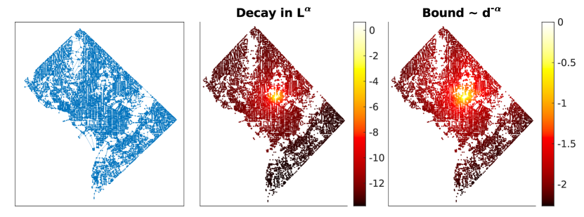
Figure 1: (Color online) Comparison between the entries of $L^{\alpha}$ and the distances between nodes in the graph DC. Left panel: largest connected component of the graph, with $n=9522$ nodes. Central panel: decay in the entries $(L^{\alpha})_{k,i_{0}}$, for $k=1,\dots,n$. Right panel: distances $d(i_{0},k)^{-\alpha}$, for $k=1,\dots,n$. We used $\alpha=0.5$ and computed $L^{\alpha}$ via its eigendecomposition (5); the scale for the colors is logarithmic.

3.2 Directed networks

Numerical evidence shows that the decay behavior in the entries of fractional Laplacians is not limited to the undirected case, but it can also be observed in directed networks; see Section 6. However, a generalization to the directed case of the results in Corollary 3.7 is not straightforward.

If $A$ is a nonnormal matrix and $f$ is analytic on an open set containing the numerical range $W(A)$ of $A$,

$$W(A)=\left\{\frac{\mathbf{x}^{H}A\mathbf{x}}{\mathbf{x}^{H}\mathbf{x}}\,:\,\mathbf{x}\in\mathbb{C}^{n},\;\mathbf{x}\neq\mathbf{0}\right\}=\left\{\mathbf{x}^{H}A\mathbf{x}\,:\,\mathbf{x}\in\mathbb{C}^{n},\;\|\mathbf{x}\|_{2}=1\right\},$$

it is shown in [3] that one can bound the entries of $f(A)$ using the following result of Crouzeix [9, 10]:

$$\exists\,C\text{ such that }\|f(A)\|_{2}\leq C\sup_{w\in W(A)}|f(w)|,$$ (10)

where $C$ is a universal constant independent of both $f$ and $A$; currently, the best known value for $C$ is $1+\sqrt{2}$, and it is conjectured to be 2. Unfortunately, (10) cannot be used in our case since $f(x)=x^{\alpha}$, $\alpha\in(0,1)$, is not analytic on the negative real axis, and it is easy to find directed graphs such that the numerical range $W(L_{\text{out}})$ of the out–degree Laplacian contains part of the negative real axis. Indeed, [17, Theorem 1.6.6] states that if $\lambda$ is an eigenvalue of $L_{\text{out}}$ that lies on the boundary of $W(L_{\text{out}})$, then the eigenvector associated to it is orthogonal to all the other eigenvectors. Thus, if $W(L_{\text{out}})\subseteq\mathbb{C}^{+}$ we have that $0\in\lambda(L_{\text{out}})\cap\partial W(L_{\text{out}})$, and then its eigenvector ${\bf 1}$ is orthogonal to all the other eigenvectors of $L_{\text{out}}$. Digraphs in which this does not happen are easy to find, and frequently encountered in applications.

Example 3.12.

Consider the graph with adjacency matrix

$$A=\begin{bmatrix}0&1&0\\ 0&0&1\\ 1&1&0\\ \end{bmatrix},$$

whose out–Laplacian $L_{\text{out}}$ has the following field of values:

$W(L_{\text{out}})=$

$$L_{\text{out}}=\begin{bmatrix}1&-1&0\\ 0&1&-1\\ -1&-1&2\\ \end{bmatrix},$$

which includes part of the negative real axis and therefore the origin.

There are other possible general alternatives to (10), which use extensions of the well known Dunford–Taylor integral representation of $f$, but attempts to bound the norm of terms like $|f(z)|=|z|^{\alpha}$, $\alpha\in(0,1)$ inside the contour integral cannot give a finite value and are not reported here.

Nevertheless, there are special cases for which a reasonable bound can be provided. First, if the Laplacian matrix is diagonalizable and we can give a bound for the spectral condition number of an eigenvector matrix that does not explode with the size of the graph, then we can prove a bound for the entries of the fractional Laplacian using an argument similar to the undirected case (Proposition 3.4). This is completely analogous to the approach taken in [3] in the case of analytic functions of nonsymmetric matrices. Of course, now the constant $c$ in the bounds (8) and (9) should also include a bound for the condition number of an eigenvector matrix diagonalizing the Laplacian $L$. Another possibility is to give up the search for general bounds and to look at special cases for which we can find explicit (closed form) expressions for the entries of $L_{\text{out}}^{\alpha}$ (and their limit for $n\rightarrow\infty$), and from these obtain estimates for the probability of a given transition on the graph. This is the case of the directed cycle and path graphs; see Section 5.

We found that, for a large enough cycle, the transition probabilities exhibit a power law decay parametrized by $\alpha$, in agreement with the bounds of Section 3.1; see Section 5 for details. In particular, similar to what happens for undirected networks, we show in Section 6 that fractional diffusion-based random walks on directed graphs result in more efficient navigation of certain complex directed networks than using the local ones.

4 Superdiffusive processes on infinite graphs

In [12, 13] Estrada et al. introduced a generalization of the diffusion equation on graphs, based on the $k$–path Laplacian, and they proved that the dynamics generated using the Mellin–transformed $k$–path Laplacian are superdiffusive processes on the infinite one– and two–dimensional lattice graphs. In this section we exploit similar techniques to prove that the dynamics generated by the fractional Laplacians $L^{\alpha}$ are superdiffusive on an infinite one–dimensional graph, both in the undirected and directed case.

Consider a time–dependent probability distribution $u(t)_{k}$, $k\in\mathbb{Z}$, such that $u(0)_{k}=\delta_{0k}$, i.e. the distribution at time $t=0$ is concentrated in $0$. The mean square displacement (MSD) of the distribution is defined as

$$\text{MSD}=\langle{\lvert u(t)-u(0)\rvert}^{2}\rangle=\sum_{k\in\mathbb{Z}}k^{2}u(t)_{k}.$$

We say that a process is superdiffusive if it generates probability distributions such that $\text{MSD}\sim ct^{\tau}$ with $\tau>1$ and $c>0$, for $t\to\infty$. In order to prove that the fractional diffusion dynamics on the infinite one–dimensional graph are superdiffusive, following the discussion in [12], we first show that by appropriately rescaling the solution $u(t)$, it converges to a stable probability distribution (Definition 4.1). Then, we will use some known properties of the limiting distribution to collect information on the behavior of the MSD of $u(t)$.

Definition 4.1 (Stable distribution).

Let $\alpha\in{(0,2]}$, $\beta\in[-1,1]$, $\gamma>0$, $\delta\in\mathbb{R}$ and

$$\omega(z,\alpha)=\begin{cases}-\tan(\alpha\frac{\pi}{2})&\text{if }\alpha\neq 1,\\ \frac{2}{\pi}\ln\left|z\right|&\text{if }\alpha=1.\end{cases}$$

A real random variable $X$ is called stable if its characteristic function can be written as

$$\mathbb{E}[e^{izX}]=\phi(z;\alpha,\beta,\gamma,\delta)=\exp\left[i\delta z-\left|\gamma z\right|^{\alpha}(1+i\beta\operatorname{sign}(z)\omega(z,\alpha))\right].$$

This means that the density of $X$ is given by

$$f(\xi;\alpha,\beta,\gamma,\delta)=\frac{1}{2\pi}\int_{-\infty}^{\infty}e^{-i\xi z}\,\phi(z;\alpha,\beta,\gamma,\delta)\,\text{d}z.$$

In the following, we will only use stable distributions with $\beta\in\{0,1\}$ and $\delta=0$, so we simplify the general notation to $f_{\beta}(\xi;\alpha,\gamma)\equiv f(\xi;\alpha,\beta,\gamma,\delta)$.

4.1 Undirected path graph

We start by examining the case of an infinite undirected path graph, i.e. the graph $G=(V,E)$ whose nodes are $V=\mathbb{Z}$ and whose edges are $E=\{(k,k\pm 1):k\in\mathbb{Z}\}$. In this case the adjacency and Laplacian matrices correspond respectively to the operators

$$(Au)_{k}=u_{k-1}+u_{k+1},\qquad u\in\ell^{2}(\mathbb{Z}),$$

and

$$(Lu)_{k}=2u_{k}-u_{k-1}-u_{k+1},\qquad u\in\ell^{2}(\mathbb{Z}).$$

For $\alpha\in(0,1)$, we consider the fractional diffusion equation on $G$ with initial condition concentrated on the vertex indexed by $0$, i.e., the bi-infinite vector $e^{(0)}$ with 1 in position 0 and 0 everywhere else,

$$\begin{cases}\displaystyle\frac{\text{d}}{\text{d}t}u(t)=-L^{\alpha}u(t),\\ u(0)=e^{(0)}.\end{cases}$$ (11)

As a first step, we find an explicit integral representation of the $k$th component $u(t)_{k}$ of the solution $u(t)$ of (11). This can be obtained by using the Fourier operator $\mathfrak{F}:\ell^{2}(\mathbb{Z})\to L^{2}(-\pi,\pi)$ and its inverse $\mathfrak{F}^{-1}:L^{2}(-\pi,\pi)\to\ell^{2}(\mathbb{Z})$,

$$(\mathfrak{F}u)\,(\theta)=\frac{1}{\sqrt{2\pi}}\sum_{k\in\mathbb{Z}}e^{ik\theta}u_{k},\quad u\in\ell^{2}(\mathbb{Z}),\qquad(\mathfrak{F}^{-1}g)_{k}=\frac{1}{\sqrt{2\pi}}\int_{-\pi}^{\pi}e^{-ikx}g(x)\,\text{d}x,\quad g\in L^{2}(-\pi,\pi).$$

Lemma 4.2.

The solution $u(t)$ to (11) is given by

$$u(t)_{k}=\frac{1}{2\pi}\int_{-\pi}^{\pi}e^{-ikx}\,e^{-t(2-2\cos x)^{\alpha}}\,\text{d}x,\qquad k\in\mathbb{Z}.$$ (12)

Proof 4.3.

It holds

$$(\mathfrak{F}Au)\,(\theta) =\frac{1}{\sqrt{2\pi}}\sum_{k\in\mathbb{Z}}e^{ik\theta}(Au)_{k}=\frac{1}{\sqrt{2\pi}}\sum_{k\in\mathbb{Z}}e^{ik\theta}(u_{k-1}+u_{k+1})=\frac{1}{\sqrt{2\pi}}\sum_{k\in\mathbb{Z}}(e^{i(k-1)\theta}+e^{i(k+1)\theta})u_{k}$$

$$=(e^{-i\theta}+e^{i\theta})\,(\mathfrak{F}u)(\theta)=2\cos\theta\,(\mathfrak{F}u)(\theta),$$

and thus $(\mathfrak{F}Lu)\,(\theta)=\left(2-2\cos\theta\right)\mathfrak{F}u(\theta)$. If we define $g=\mathfrak{F}u\in L^{2}(-\pi,\pi)$, then we have

$$(\mathfrak{F}L\mathfrak{F}^{-1}g)\,(\theta)=(2-2\cos\theta)g(\theta).$$

We have therefore proved that $L$ is conjugated to the operator on $L^{2}(-\pi,\pi)$ that multiplies functions by $a(\theta)=2-2\cos\theta$. In turn, this implies that $e^{-tL^{\alpha}}$ is conjugated to the multiplication by $a_{\alpha}(\theta)=e^{-ta(\theta)^{\alpha}}$. So, using the notation $g^{(0)}=\mathfrak{F}e^{(0)}$, the solution to (11) can be expressed as

$$u(t)_{k} =\left(e^{-tL^{\alpha}}u(0)\right)_{k}=\left(\mathfrak{F}^{-1}(a_{\alpha}g^{(0)})\right)_{k}=\frac{1}{\sqrt{2\pi}}\int_{-\pi}^{\pi}e^{-ikx}a_{\alpha}(x)g^{(0)}(x)\,\text{d}x$$

$$=\frac{1}{\sqrt{2\pi}}\int_{-\pi}^{\pi}e^{-ikx}e^{-t(2-2\cos x)^{\alpha}}(\mathfrak{F}e^{(0)})(x)\,\text{d}x=\frac{1}{{2\pi}}\int_{-\pi}^{\pi}e^{-ikx}e^{-t(2-2\cos x)^{\alpha}}\sum_{n\in\mathbb{Z}}e^{inx}\,(e^{(0)})_{n}\,\text{d}x.$$

Since the components of the initial condition are $(e^{(0)})_{n}=\delta_{0n}$, the previous expression simplifies to

$$u(t)_{k} =\frac{1}{2\pi}\int_{-\pi}^{\pi}e^{-ikx}e^{-t(2-2\cos x)^{\alpha}}\,\text{d}x.$$

We mention that Lemma 4.2 can also be found as [23, Theorem 1.3 (ii)]. We have included a proof in order to keep the discussion self-contained.

To prove that a properly scaled version of $u(t)$ converges to a stable distribution for $t\rightarrow\infty$, we need a Lemma from [12] linking together the expression of the solution (12) and a stable distribution in Definition 4.1 with $\beta=\delta=0$. However, we state it in a slightly more general formulation, which also introduces the asymmetry parameter $\beta\in[-1,1]$ and will be required shortly to deal with the directed case. Both the statement and the proof of the following lemma are based on Lemma 6.1 in [12].

Lemma 4.4.

Let $c>0$, $\alpha\in(0,2)$ and $\beta\in[-1,1]$ such that $\alpha\neq 1$ or $\beta=0$. Let $h:[-\pi,\pi]\to\mathbb{C}$ be a continuous function that satisfies

$$\text{Re}\,(h(x))>0 \text{for }x\in[-\pi,\pi]\setminus\{0\},$$ (13)

$$h(x)\sim c\left|x\right|^{\alpha}\left(\textstyle 1-i\beta\operatorname{sign}(x)\tan(\alpha\frac{\pi}{2})\right),\qquad \text{for }x\to 0.$$

Then

$$t^{1/\alpha}\frac{1}{2\pi}\int_{-\pi}^{\pi}e^{-it^{1/\alpha}\xi x}\,e^{-th(x)}\,\text{d}x\; \to\;\frac{1}{2\pi}\int_{-\infty}^{\infty}e^{-i\xi z}\,e^{-c\left|z\right|^{\alpha}\left(1-i\beta\operatorname{sign}(z)\tan(\alpha\frac{\pi}{2})\right)}\,\text{d}z$$ (14)

$$=f_{\beta}(\xi;\alpha,c^{1/\alpha}),$$

uniformly in $\xi\in\mathbb{R}$ as $t\to\infty$. In other words,

$$\frac{1}{2\pi}\int_{-\pi}^{\pi}e^{-it^{1/\alpha}\xi x}\,e^{-th(x)}\,\text{d}x\;=\;t^{-1/\alpha}f_{\beta}(\xi;\alpha,c^{1/\alpha})+o(t^{-1/\alpha}),$$ (15)

uniformly in $\xi\in\mathbb{R}$ as $t\to\infty$.

Proof 4.5.

For any $\xi\in\mathbb{R}$ and $t>0$, using the substitution $z=t^{1/\alpha}x$, we have

$$t^{1/\alpha}\frac{1}{2\pi}\int_{-\pi}^{\pi}e^{-it^{1/\alpha}\xi x}e^{-th(x)}\,\text{d}x=\frac{1}{2\pi}\int_{-\pi t^{1/\alpha}}^{\pi t^{1/\alpha}}e^{-i\xi z}e^{-th(t^{-1/\alpha}z)}\,\text{d}z.$$

By substituting this in (14) and using the triangle inequality, we get

$$\left|\,t^{1/\alpha}\frac{1}{2\pi}\int_{-\pi}^{\pi}e^{-it^{1/\alpha}\xi x}e^{-th(x)}\,\text{d}x-\frac{1}{2\pi}\int_{-\infty}^{\infty}e^{-i\xi z}e^{-c\left|z\right|^{\alpha}\left(1-i\beta\operatorname{sign}(z)\tan(\alpha\frac{\pi}{2})\right)}\,\text{d}z\,\right|\leq$$

$$\leq\frac{1}{2\pi}\int_{-\pi t^{1/\alpha}}^{\pi t^{1/\alpha}}\left|e^{-th(t^{-1/\alpha}z)}-e^{-c\left|z\right|^{\alpha}\left(1-i\beta\operatorname{sign}(z)\tan(\alpha\frac{\pi}{2})\right)}\right|\,\text{d}z+\frac{1}{2\pi}\int_{\mathbb{R}\setminus[-\pi t^{1/\alpha},\pi t^{1/\alpha}]}e^{-c\left|z\right|^{\alpha}}\,\text{d}z.$$

It is easy to see that the second term converges to $0$ as $t\to\infty$, so we only focus on the first term. Because of the hypothesis on the asymptotic behavior of $h(x)$, we have that

$$\frac{th(t^{-1/\alpha}z)}{c\left|z\right|^{\alpha}\left(1-i\beta\operatorname{sign}(z)\tan(\alpha\frac{\pi}{2})\right)}\to 1\qquad\text{as }t\to\infty.$$

This implies that, for any fixed $z\in\mathbb{R}$, the integrand in the first term goes to $0$ as $t\to\infty$. In order to conclude that the integral itself goes to $0$, by the Dominated Convergence Theorem it is sufficient to show that the integrand is bounded by an integrable function.

Using the continuity of $h$ in conjunction with (13), it is not hard to see that there exists $\lambda>0$ such that $\operatorname{Re}{h(x)}\geq\lambda\left|x\right|^{\alpha}$. This implies that the integrand is bounded for all $t>0$ by the integrable function $f(z)=e^{-\lambda\left|z\right|^{\alpha}}+e^{-c\left|z\right|^{\alpha}}$, concluding the proof of (14). Note that the convergence is uniform in $\xi\in\mathbb{R}$, since the bounds we have obtained are independent of $\xi$.

In order to have a cleaner statement for the next proposition, we allow the indices to be noninteger in the identity (12); in other words, we write

$$u(t)_{z}=\frac{1}{2\pi}\int_{-\pi}^{\pi}e^{-izx}\,e^{-t(2-2\cos x)^{\alpha}}\,\text{d}x,\qquad\forall\,z\in\mathbb{R}.$$

Proposition 4.6.

By scaling the solution $u(t)$ of (11) with respect to $t$, it converges to a stable probability distribution of the form $f_{0}(\xi;2\alpha,1)$ for $t\to\infty$. Specifically, for all $\xi\in\mathbb{R}$ it holds that

$$t^{1/2\alpha}(u(t))_{t^{1/2\alpha}\xi}\to f_{0}(\xi;2\alpha,1),\qquad\text{as }t\to\infty.$$

Proof 4.7.

From the expression of the solution in (12), we can write it in the form

$$u(t)_{{z}}=\int_{-\pi}^{\pi}e^{-i{z}x}e^{-th(x)}\,\text{d}x,$$

where $h(x)=a(x)^{\alpha}=(2-2\cos x)^{\alpha}=(x^{2}+o(x^{3}))^{\alpha}=\left|x\right|^{2\alpha}+o(x^{2\alpha+1})$ for $x\to 0$. Therefore, using Lemma 4.4 (with $\beta=0$) and the substitution $\xi=t^{-1/2\alpha}{z}$, we obtain

$$t^{1/2\alpha}\left(u(t)\right)_{t^{1/2\alpha}\xi}\to f_{0}(\xi;2\alpha,1),\qquad t\to\infty,$$

or, equivalently,

$$u(t)_{t^{1/2\alpha}\xi}=t^{-1/2\alpha}f_{0}(\xi;2\alpha,1)+o(t^{-1/2\alpha})\qquad\text{for }t\to\infty.$$ (16)

We complete our analysis of the (behavior of the) solution for $t\to\infty$ by showing that the $\text{MSD}\sim ct^{\tau}$ with $\tau>1$ and $c>0$, i.e., that we have superdiffusion. Observe now that, in our situation, the limiting stable distribution has an infinite variance since $2\alpha\in(0,2)$, thus we cannot compute the MSD of the solution directly. Let us look instead at the asymptotic behavior of the square of the full width at half maximum (FWHM) of the solution, since $\text{FWHM}^{2}$ gives a lower bound for the MSD; we recall that the FWHM can be defined as

$$\text{FWHM}=\max\left\{\left|b-a\right|:f(\xi)\geq{\textstyle\frac{1}{2}}\max_{x\in\mathbb{R}}f(x),\;\forall\,\xi\in[a,b]\right\}.$$

Theorem 4.8.

The fractional diffusion process on the infinite undirected path graph is superdiffusive for all $\alpha\in(0,1)$. In particular, the mean square displacement of the solution satisfies $\text{MSD}\geq\tilde{c}t^{1/\alpha}$, as $t\to\infty$.

Proof 4.9.

Let $\xi_{0}\in\mathbb{R}$ be such that $f_{0}(\xi_{0};2\alpha,1)=\frac{1}{2}f_{0}(0;2\alpha,1)$, so that the full width at half maximum of the distribution $f$ is $\text{FWHM}\{f(\xi)\}=2\xi_{0}$. Recalling equation (16) and using the fact that the FWHM is invariant under vertical scalings, we have that

$$\text{FWHM}\{u(t)_{k}\} =t^{1/2\alpha}\,\text{FWHM}\{u(t)_{t^{1/2\alpha}k}\}$$

$$=t^{1/2\alpha}\,\text{FWHM}\{t^{-1/2\alpha}f_{0}(k;2\alpha,1)+o(t^{-1/2\alpha})\}$$

$$=t^{1/2\alpha}\,\text{FWHM}\{f_{0}(k;2\alpha,1)+o(1)\}$$

$$\sim t^{1/2\alpha}\,2\xi_{0},\quad\qquad t\to\infty.$$

Therefore $\text{FWHM}^{2}\sim 2\xi_{0}\,t^{1/\alpha}$ and, since $\alpha\in(0,1)$, we have that $\text{FWHM}^{2}\sim c\,t^{\tau}$ with $\tau>1$. Thus we also have $\text{MSD}\geq\tilde{c}\,t^{\tau}$, i.e., the process is superdiffusive.

4.2 Directed path graph

In this part, we perform the same analysis for the fractional diffusion equation on the infinite directed path graph, i.e. the graph $G=(V,E)$ with nodes $V=\mathbb{Z}$ and edges $E=\{(k,k+1):k\in\mathbb{Z}\}$. Similarly to the undirected case, the solution converges to a stable distribution when appropriately scaled, and we can use this fact to describe the behavior of the MSD of the solution for $t\to\infty$.

We first observe that on a directed graph the diffusion equation uses the transpose of the nonsymmetric Laplacian $L_{\text{out}}$ instead of $L_{\text{out}}$. Indeed, the solution for the dynamics induced by $L_{\text{out}}^{T}$ remains a probability vector at all times since $L_{\text{out}}^{T}\bm{1}=\bm{0}$; on the other hand, this property is not preserved by the dynamics induced by $L_{\text{out}}$, since in general $\bm{1}^{T}L_{\text{out}}\neq\bm{0}^{T}$. Using $L$ to denote the transpose of the out-degree Laplacian of $G$ for simplicity of notation, the fractional diffusion equation on a directed graph is

$$\begin{cases}\displaystyle\frac{\text{d}}{\text{d}t}u(t)=-L^{\alpha}u(t),\qquad\alpha\in(0,1),\\ u(0)=e^{(0)},\end{cases}$$ (17)

where the initial condition is the one with all the mass concentrated on the vertex $0$, i.e. $(e^{(0)})_{k}=\delta_{0k}$. The (transposes of the) adjacency and Laplacian matrices correspond respectively to:

$$(Au)_{k} =u_{k-1}, \quad u\in\ell^{2}(\mathbb{Z}),$$

$$(Lu)_{k} =u_{k}-u_{k-1}, \quad u\in\ell^{2}(\mathbb{Z}).$$

Lemma 4.10.

The solution $u(t)$ to (17) is given by

$$u(t)_{k}=\frac{1}{2\pi}\int_{-\pi}^{\pi}e^{-ikx}e^{-t(1-e^{ix})^{\alpha}}\,\text{d}x.$$ (18)

Proof 4.11.

It holds

$$(\mathfrak{F}Au)\,(\theta) =\frac{1}{\sqrt{2\pi}}\sum_{k\in\mathbb{Z}}e^{ik\theta}(Au)_{k}=\frac{1}{\sqrt{2\pi}}\sum_{k\in\mathbb{Z}}e^{ik\theta}u_{k-1}$$

$$=\frac{1}{\sqrt{2\pi}}\sum_{k\in\mathbb{Z}}e^{i(k+1)\theta}u_{k}=e^{i\theta}\,(\mathfrak{F}u)(\theta).$$

Therefore we get $(\mathfrak{F}Lu)\,(\theta)=\left(1-e^{i\theta}\right)\mathfrak{F}u(\theta)$. If we define $g=\mathfrak{F}u\in L^{2}(-\pi,\pi)$, we have

$$(\mathfrak{F}L\mathfrak{F}^{-1}g)\,(\theta)=(1-e^{i\theta})g(\theta).$$

So $L$ is conjugated to the operator on $L^{2}(-\pi,\pi)$ that multiplies functions by $a(\theta)=1-e^{i\theta}$, and this implies that $e^{-tL^{\alpha}}$ is conjugated to the multiplication by $a_{\alpha}(\theta)=e^{-ta(\theta)^{\alpha}}$. Using the notation $g^{(0)}=\mathfrak{F}e^{(0)}$, we can write the solution to (17) explicitly in the form

$$u(t)_{k} =\left(e^{-tL^{\alpha}}e^{(0)}\right)_{k}=\left(\mathfrak{F}^{-1}(a_{\alpha}g^{(0)})\right)_{k}=\frac{1}{\sqrt{2\pi}}\int_{-\pi}^{\pi}e^{-ikx}a_{\alpha}(x)g^{(0)}(x)\,\text{d}x$$

$$=\frac{1}{\sqrt{2\pi}}\int_{-\pi}^{\pi}e^{-ikx}e^{-t(1-e^{ix})^{\alpha}}\mathfrak{F}e^{(0)}(x)\,\text{d}x=\frac{1}{{2\pi}}\int_{-\pi}^{\pi}e^{-ikx}e^{-t(1-e^{ix})^{\alpha}}\sum_{n\in\mathbb{Z}}e^{inx}(e^{(0)})_{n}\,\text{d}x$$

$$=\frac{1}{2\pi}\int_{-\pi}^{\pi}e^{-ikx}e^{-t(1-e^{ix})^{\alpha}}\,\text{d}x.$$

The result in Lemma 4.10 is a particular instance of a question with a long history concerning the “non-integer orders of summability” in the Cesàro sense; see, e.g., the seminal paper by Chapman [7, Parts III, and IV]. The question of the convergence of $-L^{\alpha}u$ for general sequences of complex numbers have been addressed in [22, Theorem 1]. Thus, although the expression in (18) was already known, see the discussion in [1, Section 1], we decided to give it here explicitly and with full details for the sake of keeping the discussion self-contained.

Note that as $x\to 0$ we have $(1-e^{ix})^{\alpha}\sim(-ix)^{\alpha}\sim\left|x\right|^{\alpha}\left(\cos(\alpha\frac{\pi}{2})-i\operatorname{sign}(x)\sin(\alpha\frac{\pi}{2})\right)$.

We can now use Lemma 4.4 to prove that the solution $u(t)$ converges to a stable distribution if appropriately scaled. Similar to what we did in the undirected case, for ease of notation we expand identity (18) to also include noninteger indices; that is, we write

$$u(t)_{z}=\frac{1}{2\pi}\int_{-\pi}^{\pi}e^{-izx}e^{-t(1-e^{ix})^{\alpha}}\,\text{d}x,\qquad\forall\,z\in\mathbb{R}.$$

Proposition 4.12.

By scaling the solution $u(t)$ of (17) with respect to $t$, it converges to a stable probability distribution of the form $f_{1}(\xi;\alpha,c)$ for $t\to\infty$, where $c=\cos(\alpha\frac{\pi}{2})$. Specifically, for all $\xi\in\mathbb{R}$ it holds that

$$t^{1/\alpha}(u(t))_{t^{1/\alpha}\xi}\to f_{1}(\xi;\alpha,c),\qquad\text{as }t\to\infty.$$

Proof 4.13.

In the expression for the solution (18) we have

$$h(x)=(1-e^{ix})^{\alpha}\sim\textstyle\cos({\alpha}\frac{\pi}{2})\left|x\right|^{\alpha}\left(1-i\operatorname{sign}(x)\tan(\alpha\frac{\pi}{2})\right),\qquad x\to 0.$$

Using Lemma 4.4 and introducing for simplicity of notation $c=\cos({\alpha}\frac{\pi}{2})^{1/\alpha}$, we get that for all $\xi\in\mathbb{R}$,

$$t^{1/\alpha}\left(u(t)\right)_{t^{1/\alpha}\xi}\to f_{1}(\xi;\alpha,c),\qquad t\to\infty,$$

or equivalently

$$u(t)_{t^{1/\alpha}\xi}=t^{-1/\alpha}f_{1}(\xi;\alpha,c)+o(t^{-1/\alpha}),\qquad t\to\infty.$$ (19)

As in the undirected case, the limiting stable distribution has an infinite variance since $\alpha<2$, so we cannot compute the MSD of the solution directly, and we instead examine the behavior of the square of the FWHM of the solution.

Theorem 4.14.

The full width at half maximum of the solution of the fractional diffusion process on the infinite directed path graph satisfies $\text{FWHM}^{2}\sim\tilde{c}t^{2/\alpha}$, as $t\to\infty$.

Proof 4.15.

Let $\xi_{0}\in\mathbb{R}$ be such that $f_{1}(\xi_{0};\alpha,c)=\frac{1}{2}f_{1}(0;\alpha,c)$, so that the full width at half maximum of the distribution $f_{1}$ is $\text{FWHM}\{f_{1}(\xi)\}=\xi_{0}$ (note that the density $f_{1}$ is nonsymmetric and identically $0$ for $\xi<0$). Recalling equation (19) and using the fact that the FWHM is invariant under vertical scalings, we have

$$\text{FWHM}\{u(t)_{k}\} =t^{1/\alpha}\,\text{FWHM}\{u(t)_{t^{1/\alpha}k}\}$$

$$=t^{1/\alpha}\,\text{FWHM}\{t^{-1/\alpha}f_{1}(k;\alpha,c)+o(t^{-1/\alpha})\}$$

$$=t^{1/\alpha}\,\text{FWHM}\{f_{1}(k;\alpha,c)+o(1)\}$$

$$\sim t^{1/\alpha}\,\xi_{0},\quad\qquad t\to\infty.$$

Therefore we obtain $\text{FWHM}^{2}\sim\xi_{0}^{2}\,t^{2/\alpha}$.

Note that, in contrast to Theorem 4.8, with Theorem 4.14 we have proved that the fractional diffusion dynamics on the infinite directed path graph is “superdiffusive” for all $\alpha\in(0,2)$; in particular, this holds also for classical diffusion, $\alpha=1$. This behavior seems at first sight confusing, but it can be explained by observing that the interpretation of (17) as describing a diffusion process is not appropriate. Indeed, the probability distribution is not really subjected to a diffusion process, since it is always “pushed” in the same direction in the graph; in other words, this process is more similar to a fractionalization of advection (or transport) than of diffusion. This can also be observed by comparing the definitions of the Laplacians of the undirected and directed path graphs: while the former one corresponds to a centered discretization of the second derivative in space (diffusion), the latter one corresponds to a forward discretization of the first derivative in space (advection).

In conclusion, we have proved that the solution to the fractional “diffusion” dynamics (17) on the directed path graph expands faster than the classical dynamics, similarly to what we proved in the undirected case; however, we cannot directly compare the directed case with the undirected one, since they can be respectively interpreted as advection and diffusion, and thus they have different time scales.

5 Closed form expressions for two simple cases

Having defined the fractional $\alpha$th power of the matrix $L_{\text{out}}$, we consider the normalized version of $\bar{L}_{\text{out}}^{(\alpha)}$ with entries $(L_{\text{out}}^{\alpha})_{i,j}/(L_{\text{out}}^{\alpha})_{i,i}$. It can then be exploited to generate the discrete time dynamics of a random walker on a directed graph by considering the transition matrix $P_{\text{out}}^{(\alpha)}=I-\bar{L}_{\text{out}}^{(\alpha)}$. As in the symmetric case discussed in [28] and in Lemma 3.1, this matrix is a row stochastic matrix, and the standard transition matrix for the Laplacian $L_{\text{out}}$ is recovered as $\alpha\rightarrow 1$.

To completely describe the behavior of the random walker in a fully analytical setting we consider two test cases, the directed path $\mathcal{P}_{n}$, and the directed cycle graph $\mathcal{C}_{n}$.

The directed path $\mathcal{P}_{n}$ is the graph with adjacency matrix $A=(a_{i,j})$ with $a_{i,i+1}=1$, $i=1,\ldots,n-1$, and whose outdegree Laplacian $L_{\text{out}}$ is

$$L_{\text{out}}=\begin{bmatrix}1&-1\\ &1&-1\\ &&\ddots&\ddots\\ &&&1&-1\\ &&&&0\end{bmatrix}.$$

This is a nonsymmetric, nondiagonalizable matrix, thus we cannot apply decomposition (5), and we need to use Definition 2.2. Therefore, we first need to compute the Jordan canonical form of $L_{\text{out}}=ZJZ^{-1}$, that reads as

$$Z=\begin{bmatrix}1&-1&&\\ 1&&1&\\ \vdots&&&\ddots\\ 1&&&&&(-1)^{n-1}\\ 1&&&&&0\end{bmatrix},\quad J=\begin{bmatrix}0&&\\ &1&1\\ &&\ddots&\ddots\\ &&&\ddots&1\\ &&&&1\\ \end{bmatrix}.$$

Thus, the resulting matrix function can be expressed by computing

$$J^{\alpha}=\begin{bmatrix}0&0&\cdots&0\\ &\binom{\alpha}{0}&\cdots&\binom{\alpha}{n-1}\\ &&\ddots&\vdots\\ &&&\binom{\alpha}{0}\\ \end{bmatrix},\quad\binom{\alpha}{k}=\frac{\alpha\cdot\ldots\cdot(\alpha-k+1)}{k!},$$

and by expressing $L_{\text{out}}^{\alpha}=ZJ^{\alpha}Z^{-1}$. So for $h\geq 1$ and $k<n$ we can express its $(h,k)$ element as

$$(L_{\text{out}}^{\alpha})_{h,k}=\begin{cases}0,&\text{ if }k<h\text{ or }k=h=n,\\ -1,&\text{ if }(h,k)=(n-1,n),\\ (-1)^{h+k}\binom{\alpha}{k-h},&\text{ if }1\leq h\leq k\leq n-1.\end{cases}$$

Therefore, the probability $p_{h\to k}^{(\alpha)}$ of a transition $h\to k$ on the directed path graph is given by

$$p_{h\to k}^{(\alpha)}=\begin{cases}0,&h=n,\\ \delta_{h,k}-\frac{(L_{\text{out}}^{\alpha})_{h,k}}{(L_{\text{out}}^{\alpha})_{h,h}}=\delta_{h,k}-(L_{\text{out}}^{\alpha})_{h,k},&\text{otherwise}.\end{cases}$$

If we let the size of the graph $n$ grow to infinity, and consider the decay of the transition probability for large values of $k>h$ we observe that

$$p_{h\to k}^{(\alpha)}=-\frac{\Gamma(k-h-\alpha)}{\Gamma(-\alpha)\Gamma(k-h+1)}\sim\frac{\Gamma(\alpha+1)\sin(\pi\alpha)}{\pi}k^{-\alpha-1},\quad\text{ since }\frac{\Gamma(x+\alpha)}{\Gamma(x+\beta)}\sim x^{a-b}\text{ as }x\rightarrow+\infty,$$

i.e., a polynomial decay parameterized by $\alpha$. Note that the associated chain has an absorbing state (the last vertex), which is always reached. Therefore, the effect of the nonlocality is reflected by the fact that we have a higher probability of transitioning to a far away node without completely exploring the network. In Figure 2, we observe the simulated behavior for 10 steps on a directed path with $n=20$ nodes, always starting from the first one.

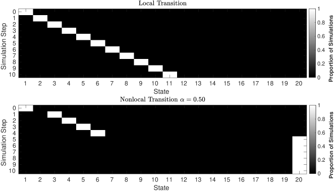
Figure 2: Simulation of $10$ steps of the local and nonlocal ($\alpha=0.5$) Markov chains on the directed path with $n=20$ nodes. In both cases we start from the first node of the chain, when $\alpha=0.5$ we reach the absorbing state in $5$ steps, which is exactly the value predicted by (20).

Moreover, decreasing the value of $\alpha$ resolves in faster absorption. To compute the average number of steps needed to reach the absorbing state starting from the first node, we partition the matrix $L^{\alpha}_{\text{out}}$ into the block form

$$L^{\alpha}=\begin{bmatrix}I-Q&\mathbf{r}\\ \mathbf{0}&0\end{bmatrix},$$

to extract the inverse of the fundamental matrix $I-Q$. Then we can compute the expected number of steps $n_{\text{step}}$ [21, Theorem 3.3.5] as $n_{\text{step}}=\lceil(I-Q)^{-1}\mathbf{1})_{1}\rceil$. By reusing the computation done for $J^{\alpha}$, it is easy to prove that $(I-Q)^{-1}$ is the upper triangular Toeplitz matrix with first row $(\mathbf{t})_{\ell}=t_{\ell}=(-1)^{\ell-1}\binom{-\alpha}{\ell-1}$, $\ell=1,\ldots,n-1$. Therefore, the expected number of steps needed to reach the absorbing state starting from the first node is

$$\begin{split}n_{\text{step}}=&\;\left\lceil\sum_{\ell=1}^{n-1}(-1)^{\ell-1}\binom{-\alpha}{\ell-1}\right\rceil=\left\lceil\frac{(-1)^{n+1}(n-1)\binom{-\alpha}{n-1}}{\alpha}\right\rceil,\end{split}$$ (20)

which is a monotonically increasing function with respect to $\alpha$.

For the case of the directed cycle graph $\mathcal{C}_{n}$, i.e., of the graph with nodes $V=\{1,\ldots,n\}$ and directed edges $E=\{(j,j+1),\,j=1,\ldots,n-1\}\cup\{(n,1)\}$, the out-degree Laplacian is then the circulant matrix of size $n$ with first row $\mathbf{c}=[1,-1,0,\ldots,0]$, i.e., $(L_{\text{out}})_{i,j}=c_{j-i\text{(mod }n\text{)}}$. This is a normal matrix which is diagonalized by the discrete Fourier matrix of size $n$, $F_{n}$, and whose eigenvalues are given by $\lambda_{\ell}(L_{\text{out}})=1-\exp(-{2\ell i\pi}/{n})$. By using (5) for this particular out-degree Laplacian we find

$$(L_{\text{out}}^{\alpha})_{h,k}=\frac{1}{n}\sum_{\ell=1}^{n}\left(1-e^{\frac{-2\ell\pi\cdot i}{n}}\right)^{\alpha}e^{\frac{2\ell\pi\cdot i}{n}(h-k)}.$$

Taking the limit for $n\rightarrow+\infty$ we can then express the $(h,k)$ element of $L_{\text{out}}^{\alpha}$ as

$$\begin{split}(L_{\text{out}}^{\alpha})_{h,k}=\;\frac{1}{2\pi}\int_{0}^{2\pi}(1-e^{-i\theta})^{\alpha}e^{id_{h,k}\theta}\,d\theta=\;\frac{\Gamma(d_{h,k}-\alpha)}{d_{h,k}!\Gamma(-\alpha)},\end{split}$$

where $d_{h,k}=h-k\,(\operatorname{mod}\,n)$. Therefore, the probability $p_{h\to k}^{(\alpha)}$ of a $h\to k$ transition on the cycle graph is given by

$$p_{h\to k}^{(\alpha)}=\delta_{h,k}-\frac{(L_{\text{out}}^{\alpha})_{h,k}}{(L_{\text{out}}^{\alpha})_{h,h}}=\delta_{h,k}-\frac{\Gamma(d_{h,k}-\alpha)}{d_{h,k}!\Gamma(-\alpha)}.$$

For $h,k$ such that $d_{h,k}\gg 1$ we can expand this transition probability, for $\alpha\in(0,1)$, as

$$p_{h\to k}^{(\alpha)}=-d_{h,k}^{-\alpha}\left(\frac{1}{d_{h,k}\Gamma(-\alpha)}+O\left(\frac{1}{d_{h,k}^{2}}\right)\right)\approx-\frac{d_{h,k}^{-\alpha-1}}{\Gamma(-\alpha)},$$

thus showing that, for a large enough cycle, the transition probability behaves as a distribution whose probabilities decay polynomially with respect to $\alpha$. In this case the underlying graph is strongly connected, therefore we do not have any absorbing states in the chain. In the local dynamics case, we can be sure that in a number of steps equal to the number of nodes of the network we completely explore it, while, on the other hand, the possibility of performing longer jumps increases the probability of returning to certain states while leaving others untouched. See, e.g., the example in Figure 3 for a directed cycle graph with $n=20$ nodes in which $10$ jumps are performed.

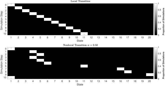
Figure 3: Simulation of $10$ steps of the local and nonlocal ($\alpha=0.25$) Markov chains on the directed cycle graph with $n=20$ nodes. In both cases we start from the same node of the cycle we identifiy with node 1.

6 Applications

The simple examples from Section 5 seem to suggest that, in the presence of a strong directionality in the network, the possibility of performing long distance jumps does not necessarily lead to better (i.e., faster) exploration of the network compared to the classical, local random walk (or, in the case of continuous time, diffusion) dynamics. Real world directed networks, however, are very different from these simple “unidirectional” graphs, and allow for far richer exploration dynamics. To understand what we have gained in moving from the standard random walk on the network to its fractional extension, we consider the efficiency of the new dynamics in exploring the underlying directed graph compared to the classical dynamics. To measure it, we consider the average return probability at time $t$, $p_{0}^{(\alpha)}(t)$, for a continuous time random walker described by the master equation for the probability $p(i,t|i_{0},0)$ of being at node $i$ at time $t$ having started from node $i_{0}$ at time $t=0$, for the dynamics induced by the normalized version of $\bar{L}_{\text{out}}^{(\alpha)}$. The continuous time random walk master equation on a directed graph reads as

$$\partial_{t}p(i,t|i_{0},0)=-\sum_{j}p(j,t|i_{0},0)(\bar{L}_{\text{out}}^{(\alpha)})_{ji},$$

with initial condition $p(i,0|i_{0},0)=\delta_{i,i_{0}}$. The desired average return probability is obtained as

$$p_{0}^{(\alpha)}(t)=\frac{1}{n}\sum_{i=1}^{n}p(i,t|i,0)=\frac{1}{n}\sum_{i=1}^{n}\exp(-\lambda_{i}(\bar{L}_{\text{out}}^{(\alpha)})t).$$

Even if $\bar{L}_{\text{out}}^{(\alpha)}$ has complex eigenvalues, they always appear in conjugate pairs. Therefore, $p_{0}^{(\alpha)}(t)$ is always a real number; specifically, we consider the network Roget in which each vertex corresponds to one of the categories in the 1879 edition of Peter Mark “Roget’s Thesaurus of English Words and Phrases”, and in which each arc connects two categories whenever Roget give reference to one of them among the words and phrases of the other, or if the two categories are directly related by their positions in the book. The wiki-Vote network containing all the Wikipedia voting data from the 2,794 elections that had taken place till January 2008. Nodes in the network represent Wikipedia users, directed arcs from node $i$ to node $j$ exists whenever user $i$ voted for user $j$. The network p2p-Gnutella08 obtained from the eight of the nine snapshots of the Gnutella peer-to-peer file sharing network collected in August 2002. In this case, the nodes are the hosts in the Gnutella network topology and the arcs are the connections between the hosts. For all the three cases, we restrict to the largest connected component of the network. The following examples demonstrate that in the case of real world complex digraphs, the use of nonlocal diffusion processes (or random walks) display similar advantages to those observed in the undirected case. We report in Figure 4 the quantity $p_{0}^{(\alpha)}(t)$ while highlighting the value of the first nonzero eigenvalue of the associated Laplacian. For each network we also report the relative spectral gap (magnitude of the ratio of the largest to the smallest nonzero eigenvalue) and the network diameter.

As we can observe, the higher the spectral gap, i.e., the larger the modulus of the second smallest eigenvalue of the Laplacian matrix $L_{\text{out}}$ is, the more efficient the fractional exploration of the associated network is. This is an expected behavior since the average return probability is directly linked to the whole spectral distribution of the associated normalized Laplacian matrix. In particular, it is well known that sparse networks with larger spectral gap can be explored more efficiently than those having a smaller spectral gap. The network’s diameter, on the other hand, seems to be less relevant as an indicator of when the nonlocal dynamics is more efficient than the local one.

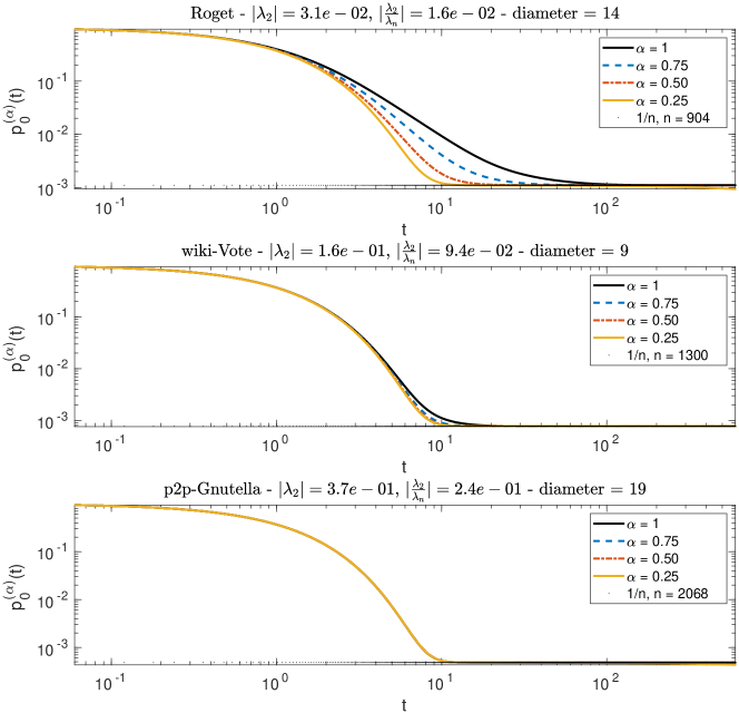
Figure 4: (Color online) Average fractional return probability $\mathbf{p}_{i}^{(\alpha)}(t)$ as a function of time for three different directed networks Roget, wiki-Vote, and p2p-Gnutella08. In each case we restrict the analysis to the largest connected component of the network. Note the logarithmic scale on the axes.

We also observe that the behavior shown in Figure 4 is similar to that observed for the fractional dynamics on undirected networks in [28].

6.1 Consensus models for control of vehicle motions

Consider an ensemble of $N$ vehicles moving in an $m$th dimensional space. We denote the initial positions by $\mathbf{x}_{i}\in\mathbb{R}^{m}$, $i=1,\ldots,N$, and the initial velocities by $\mathbf{v}_{i}\in\mathbb{R}^{m}$, $i=1,\ldots,N$. We are interested in steering the vehicles from their initial position to a prefixed end state, $\{(\mathbf{x}^{*}(t),\mathbf{v}^{*}(t))\in\mathbb{R}^{Nm\times Nm}\,:\,\dot{\mathbf{x}}^{*}(t)=\mathbf{v}^{*}(t),$ for all $t\geq T_{\text{final}}\}$, while maintaining fixed the geometric configuration between them. Of the many available approaches for this task, we focus on the class of consensus algorithms for systems modeled by a second-order dynamics in which the communication among the various vehicles is described in terms of the Laplacian of the graph of their connections. Specifically, we consider the following consensus model from [27]:

$$\left\{\begin{array}[]{rl}\dot{\mathbf{x}}_{i}=&\mathbf{v}_{i},\\ \dot{\mathbf{v}}_{i}=&\ddot{\mathbf{x}}^{*}_{i}-\beta(\mathbf{x}_{i}-\mathbf{x}_{i}^{*})-\gamma\beta(\mathbf{v}_{i}-\dot{\mathbf{x}}_{i}^{*})\\ &-\sum_{j=1}^{N}L_{i,j}[(\mathbf{x}_{i}-\mathbf{x}_{i}^{*})-(\mathbf{x}_{j}-\mathbf{x}_{j}^{*})]\\ &-\gamma\sum_{j=1}^{N}L_{i,j}[(\mathbf{v}_{i}-\dot{\mathbf{x}}_{i}^{*})-(\mathbf{x}_{j}-\dot{\mathbf{x}}_{j}^{*})],\end{array}\right.$$ (21)

which can be expressed in matrix form as

$$\frac{\text{d}}{\text{d}t}{{\begin{bmatrix}\tilde{\mathbf{x}}\\ \tilde{\mathbf{v}}\end{bmatrix}}}=\left(\begin{bmatrix}O_{N\times N}&I_{N}\\ -(\beta I_{N}+L)&-\gamma(\beta I_{N}+L)\end{bmatrix}\otimes I_{m}\right){\begin{bmatrix}\tilde{\mathbf{x}}\\ \tilde{\mathbf{v}}\end{bmatrix}}$$

where $\tilde{\mathbf{x}}=\mathbf{x}^{*}-\mathbf{x}$, and $\tilde{\mathbf{v}}=\mathbf{v}^{*}-\mathbf{v}$. From Theorem 3.3 [27] we can extract the following limit result for (21).

Theorem 6.1.

Let $L$ be the Laplacian of the graph of the connections in (21). Let $\mu_{i}$ be the $i$-th eigenvalue of $-L$. Then, $\mathbf{x}\rightarrow\mathbf{x}^{*}$, $\mathbf{v}\rightarrow\mathbf{v}^{*}$ if

$$\gamma>\max_{i}\sqrt{2}\left(|\nu_{i}|\cos(\frac{\pi}{2})-\tan^{-1}\left(-\frac{\operatorname{Re}(\nu_{i})}{\operatorname{Im}(\nu_{i})}\right)\right)^{-\frac{1}{2}},$$ (22)

$\nu_{i}=-\beta+\mu_{i}$.

The model (21) is extended here by considering a fractional power of the graph Laplacian, i.e., $L^{\alpha}$, $\alpha\in(0,1)$ instead of $L$. The convergence analysis can be performed with the same tools used in [27] and gives a result analogous to Theorem 6.1 but with $\mu_{i}$ the eigenvalues of $-L^{\alpha}$. The notable differences are that now the dynamics is faster as $\alpha$ approaches $0$, together with the fact that increasing the amount of communication helps the vehicles in maintaining their formation; see the numerical experiment in Figure 5 in which it can be observed that the position at each time step of the vehicles resembles the initial one faster as $\alpha$ is smaller.

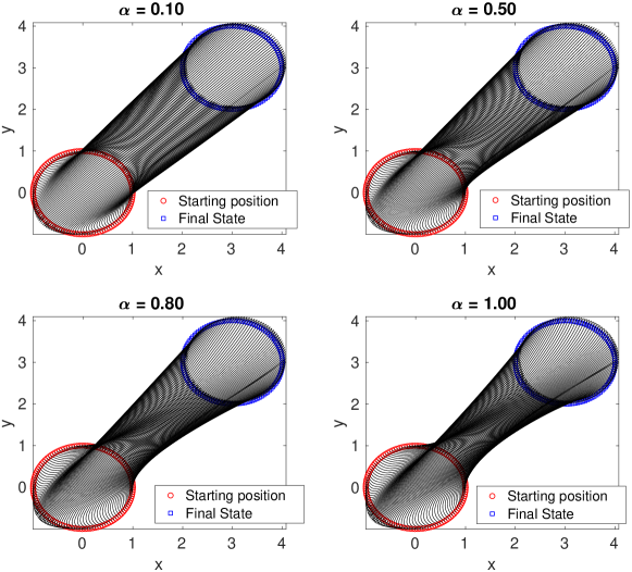
(a) Trace of the position of the vehicles

(b) Absolute error on the final position with respect to time

Figure 5: (Color online) We consider here the test cases in which $n=120$ vehicles are uniformly distributed on the unit circle $\mathbf{x}=(\cos(t_{i}),\sin(t_{i}))_{i}$, $\{t_{i}={2\pi i}{n}\}_{i=1}^{n}$, with starting velocity given $\mathbf{v}=\dot{\mathbf{x}}$, i.e., they are following a uniform circular motion. The desired ending state is represented again by a circle of unit radius and uniformly distributed vehicles but with center in $(3,3)$ and zero terminal velocity. The parameter $\beta$ is $0.5$ while $\gamma$ is computed as the lower bound in (22) plus one. The communication graph between the vehicles is the directed cycle.

7 Conclusions

In this paper we have investigated nonlocal diffusion dynamics (both discrete and continuous in time) on undirected as well as on directed networks using fractional powers of a suitable version of the graph Laplacian and its normalized counterpart. In order to treat the directed case, we have discussed the definition of the $\alpha$th power of a nonsymmetric graph Laplacian. We proved also that the proposed dynamic exhibits a superdiffusive behavior for both the undirected and directed path graph thus strengthening the analogy with the continuous fractional Laplacian. We have obtained analytical solutions for two simple directed graphs (a periodic one and an absorbing one) and highlighted some differences and similarities with fractional diffusion on related undirected graphs. Experiments on a few real world examples indicate that, similar to the undirected case, nonlocal (fractional) diffusion and related random walks on directed graphs result in more efficient navigation of complex directed networks than using the standard (local) counterparts. Finally, we have extended an existing consensus models for vehicle motions on directed networks to one driven by a fractional nonsymmetric Laplacian and observed that the system displays faster convergence to consensus than the standard (nonfractional) model.

In conclusion, the dynamics of nonlocal fractional diffusion appears to be a useful tool in the study of several problems involving directed as well as undirected graph models.

Funding

This work was supported in part by the Tor Vergata University “Beyond Borders” program through the project ASTRID, CUP E84I19002250005; by the INdAM–GNCS projects “Tecniche innovative e parallele per sistemi lineari e non lineari di grandi dimensioni, funzioni ed equazioni matriciali ed applicazioni”, “Nonlocal models for the analysis of complex networks”and “Metodi low-rank per problemi di algebra lineare con struttura data-sparse”.

References

- [1] Abadias, L., De León-Contreras, M. & Torrea, J. L. (2017) Non-local fractional derivatives. Discrete and continuous. J. Math. Anal. Appl., 449(1), 734–755.
- [2] Bauer, F. (2012) Normalized graph Laplacians for directed graphs. Linear Algebra Appl., 436(11), 4193–4222.
- [3] Benzi, M. & Boito, P. (2014) Decay properties for functions of matrices over -algebras. Linear Algebra Appl., 456, 174–198.
- [4] Benzi, M. & Razouk, N. (2007/08) Decay bounds and algorithms for approximating functions of sparse matrices. Electron. Trans. Numer. Anal., 28, 16–39.
- [5] Benzi, M. & Simoncini, V. (2015) Decay bounds for functions of Hermitian matrices with banded or Kronecker structure. SIAM J. Matrix Anal. Appl., 36(3), 1263–1282.
- [6] Berman, A. & Plemmons, R. J. (1994) Nonnegative Matrices in the Mathematical Sciences, volume 9 of Classics in Applied Mathematics. Society for Industrial and Applied Mathematics (SIAM), Philadelphia, PA. Revised reprint of the 1979 original.
- [7] Chapman, S. (1911) On Non-Integral Orders of Summability of Series and Integrals. Proc. London Math. Soc. (2), 9, 369–409.
- [8] Chung, F. (2005) Laplacians and the Cheeger inequality for directed graphs. Ann. Comb., 9(1), 1–19.
- [9] Crouzeix, M. (2004) Bounds for analytical functions of matrices. Integral Equations Operator Theory, 48, 461–477.
- [10] Crouzeix, M. (2007) Numerical range and functional calculus in Hilbert space. J. Funct. Anal., 244(2), 668–690.
- [11] Estrada, E., Delvenne, J.-C., Hatano, N., Mateos, J. L., Metzler, R., Riascos, A. P. & Schaub, M. T. (2018a) Random multi-hopper model: super-fast random walks on graphs. J. Complex Netw., 6(3), 382–403.
- [12] Estrada, E., Hameed, E., Hatano, N. & Langer, M. (2017) Path Laplacian operators and superdiffusive processes on graphs. I. One-dimensional case. Linear Algebra and Its Applications, 523, 307–334.
- [13] Estrada, E., Hameed, E., Langer, M. & Puchalska, A. (2018b) Path Laplacian operators and superdiffusive processes on graphs. II. Two-dimensional lattice. Linear Algebra and Its Applications, 555, 373–397.
- [14] Fiedler, M. & Schneider, H. (1983) Analytic functions of -matrices and generalizations. Linear and Multilinear Algebra, 13(3), 185–201.
- [15] Guo, C.-H. (2010) On Newton’s method and Halley’s method for the principal th root of a matrix. Linear Algebra Appl., 432(8), 1905–1922.
- [16] Higham, N. J. (2008) Functions of Matrices. Theory and Computation. Society for Industrial and Applied Mathematics (SIAM), Philadelphia, PA.
- [17] Horn, R. A. & Johnson, C. R. (2013) Matrix Analysis. Cambridge University Press, Cambridge, second edition.
- [18] Ilic, M., Liu, F., Turner, I. & Anh, V. (2005) Numerical approximation of a fractional-in-space diffusion equation. I. Fract. Calc. Appl. Anal., 8(3), 323–341.
- [19] Ilic, M., Liu, F., Turner, I. & Anh, V. (2006) Numerical approximation of a fractional-in-space diffusion equation. II. With nonhomogeneous boundary conditions. Fract. Calc. Appl. Anal., 9(4), 333–349.
- [20] Iserles, A. (2000) How large is the exponential of a banded matrix?. New Zealand J. Math., 29(2), 177–192. Dedicated to John Butcher.
- [21] Kemeny, J. G. & Snell, J. L. (1960) Finite Markov Chains. The University Series in Undergraduate Mathematics. D. Van Nostrand Co., Inc., Princeton, N.J.-Toronto-London-New York.
- [22] Kuttner, B. (1957) On differences of fractional order. Proc. London Math. Soc. (3), 7, 453–466.
- [23] Lizama, C. & Roncal, L. (2018) Hölder-Lebesgue regularity and almost periodicity for semidiscrete equations with a fractional Laplacian. Discrete Contin. Dyn. Syst., 38(3), 1365–1403.
- [24] Meinardus, G. (1967) Approximation of Functions: Theory and Numerical Methods. Springer, Berlin.
- [25] Metzler, R. & Klafter, J. (2000) The random walk’s guide to anomalous diffusion: a fractional dynamics approach. Phys. Rep., 339(1), 77.
- [26] Page, L., Brin, S., Motwani, R. & Winograd, T. (1999) The PageRank citation ranking: Bringing order to the web.. Technical report, Stanford InfoLab.
- [27] Ren, W. (2007) Consensus strategies for cooperative control of vehicle formations. IET Control Theory & Applications, 1, 505–512(7).
- [28] Riascos, A. P. & Mateos, J. L. (2014) Fractional dynamics on networks: Emergence of anomalous diffusion and Lévy flights. Phys. Rev. E, 90, 032809.