Edgeworth expansion with error estimates for power law shot noise

Abstract: Consider a homogeneous Poisson process in $\mathbb{R}^{d}$, $d\geq 1$. Let $R_{1}<R_{2}<\dots$ be the distances of the points from the origin, and let $S=R_{1}^{-\gamma}+R_{2}^{-\gamma}+\dots$, where $\gamma>d$ is a parameter. Let $\overline{S}^{(r)}=\sum_{k}R_{k}^{-\gamma}\,\mathbf{1}_{R_{k}\geq r}$ be the contribution to $S$ outside radius $r$. For large enough $r$, and any $\overline{s}$ in the support of $\overline{S}^{(r)}$, consider the change of measure that shifts the mean to $\overline{s}$. We derive rigorous error estimates for the Edgeworth expansion of the transformed random variable. Our error terms are uniform in $\overline{s}$, and we give explicitly the dependence of the error on $r$ and the order $k$ of the expansion. As an application, we provide a scheme that approximates the conditional distribution of $R_{1}$ given $S=s$ to any desired accuracy, with error bounds that are uniform in $s$. Along the way, we prove a stochastic comparison between $(R_{1},R_{2},\dots)$ given $S=s$ and unconditioned radii $(R^{\prime}_{1},R^{\prime}_{2},\dots)$.

Key-words: Poisson point process, positive stable law, Edgeworth expansion, change of measure, power law shot noise, pathloss

MSC 2010: 60F05

1 Introduction

Consider a homogeneous Poisson point process in $\mathbb{R}^{d}$. Let $0<R_{1}<R_{2}<\dots$ be the distances of the points from the origin in increasing order, and let

$$S=\sum_{k=1}^{\infty}R_{k}^{-\gamma}\qquad\qquad\overline{S}^{(r)}=\sum_{k:R_{k}>r}R_{k}^{-\gamma},\quad r\geq 0,$$ (1)

where $\gamma>d$ is a parameter. It is well known, and easy to see that $S=\overline{S}^{(0)}$ is a stable random variable of index $d/\gamma$ [15, Section 1.4].

1.1 Motivation

The setup above has the following interpretation relevant to wireless communication [9, Chapter 5], [18]. Assume that $d=2$ and at each point of the Poisson process a radio transmitter is located that emits a signal at unit power. The signal experiences a path loss $r^{-\gamma}$ at distance $r$ from the source, and hence an observer located at the origin receives a total signal $S$. Suppose that the observer measures $S$ and is interested in the distance $R_{1}$ to the nearest transmitter (providing the strongest signal for the observer). The density of $R_{1}$, given $S=s$, is

$$f_{R_{1}\,|\,S}(r_{1}\,|\,s)=\frac{1}{f_{S}(s)}f_{R_{1}}(r_{1})\,f_{S\,|\,R_{1}}(s\,|\,r_{1})=\frac{1}{f_{S}(s)}f_{R_{1}}(r_{1})\,f_{\overline{S}^{(r_{1})}}(s-r_{1}^{-\gamma}).$$ (2)

As no closed formula is known for the density of $\overline{S}^{(r)}$, it is of interest to find approximations. The main technical result of this paper gives rigorous error estimates for an approximation of this density when $r$ is large. This large $r$ result can be used, via a modification of (2) described further below, to approximate $f_{R_{1}\,|\,S}$ to any desired accuracy.

1.2 Approximating $\overline{S}^{(r)}$

Let us first describe the approximation to $\overline{S}^{(r)}$ we consider. We let $\mu(r)=\mathbf{E}[\overline{S}^{(r)}]$, $\sigma^{2}(r)=\mathsf{Var}(\overline{S}^{(r)})$, and

$$Y^{(r)}=\frac{\overline{S}^{(r)}-\mu(r)}{\sigma(r)}.$$

As $r\to\infty$, $Y^{(r)}$ tends to a standard Gaussian. An explicit way to see this is to write $\overline{S}^{(r)}$ as a sum of independent contributions from shells:

$$\overline{S}^{(r)}=\sum_{n=1}^{\infty}\left(\overline{S}^{(r+n-1)}-\overline{S}^{(r+n)}\right).$$

Since the volume of the $n$-th shell is $\approx c(r+n)^{d-1}$, the mean of the $n$-th term is $\approx c(r+n)^{d-1-\gamma}$ and its variance is $\approx c^{\prime}(r+n)^{d-1-2\gamma}$. Asymptotic normality of $\overline{S}^{(r)}$ can be deduced for example from Lyapunov’s criterion [5, Section X.8, Exercise 3]. We note that the mean and variance of $\overline{S}^{(r)}$ are of the form $\mu(r)=c\,r^{d-\gamma}$ and $\sigma^{2}(r)=c^{\prime}r^{d-2\gamma}$. Since the value of $\lambda$ can be fixed by scaling, we assume throughout that $\lambda$ has the fixed value that makes $c^{\prime}=1$.

Let $y$ be a fixed possible value of $Y^{(r)}$, and suppose we want to approximate the density $f_{Y^{(r)}}(y)$. We transform the variable $Y^{(r)}$ into a variable $\widetilde{Y}^{(r)}$, in such a way that the mean becomes $\mathbf{E}[\widetilde{Y}^{(r)}]=y$, and hence $y$ is ‘typical’ for $\widetilde{Y}^{(r)}$. This technique is standard in many branches of probability; see for example [6, Section XVI.7], where it is called the technique of ‘associated distributions’; or see [10, Section I.3], where it is called the ‘Cramér transform’; other names are: ‘change of measure’ and ‘tilting’. In order to define the transformation, denote the Laplace transform $\varphi_{Y^{(r)}}(t):=\mathbf{E}\left[e^{-tY^{(r)}}\right]$. The transformed probability density is

$$f_{\widetilde{Y}^{(r)}}(z):=\frac{e^{\xi z}}{\varphi_{Y^{(r)}}(-\xi)}f_{Y^{(r)}}(z),\quad z\in\mathbb{R},$$ (3)

where the parameter $\xi$ is chosen to be

$$\xi=\xi(y,r):=\operatorname*{arg\,min}_{\xi^{\prime}\in\mathbb{R}}\,e^{-\xi^{\prime}y}\varphi_{Y^{(r)}}(-\xi^{\prime}).$$ (4)

Let $\widetilde{\kappa}_{2}=\widetilde{\kappa}_{2}(y,r)$ denote the variance of $\widetilde{Y}^{(r)}$. It depends both on $r$ and $y$, through the definition of $\xi(y,r)$. The simplest approximation is to replace $\widetilde{Y}^{(r)}$ by a Gaussian of mean $y$ and variance $\widetilde{\kappa}_{2}$, which gives $f_{\widetilde{Y}^{(r)}}(y)\approx 1/\sqrt{2\pi\widetilde{\kappa}_{2}(y,r)}$. Inverting the transformation in (3), this gives an approximation of $f_{Y^{(r)}}(y)$. We find that the relative error of this approximation is uniform in $y$. That is, for all $r\geq 1$ and all $y$ in the support of the distribution of $Y^{(r)}$, we have

$$\begin{split}f_{Y^{(r)}}(y)=\frac{1}{\sqrt{2\pi\widetilde{\kappa}_{2}(y,r)}}e^{-\xi(y,r)\,y}\,\varphi_{Y^{(r)}}(-\xi(y,r))\,\left[1+O\left(r^{-d/2}\right)\right],\end{split}$$

where the constant in the error term only depends on $d$.

When $r$ is large, it is possible to improve the error, by replacing the normal approximation by the so-called Edgeworth expansion; see [6, Section XVI.2, Theorem 2]. We briefly explain the idea of this expansion, in order to state our main theorem. The normal approximation is based on a Taylor expansion of the characteristic function $\chi_{\widetilde{Y}^{(r)}}$ of $\widetilde{Y}^{(r)}$ to second order, and hence involves the mean and variance of $\widetilde{Y}^{(r)}$. When higher order moments also exists, the Taylor expansion can be continued with $k$ additional terms for some $k\geq 1$. Abreviating $\rho=r^{d/2}$, this takes the form

$$\begin{split}\chi_{\widetilde{Y}^{(r)}}(t)&=\exp\left(ity-\frac{t^{2}}{2!}\widetilde{\kappa}_{2}+\frac{(it)^{3}}{3!}\frac{\widetilde{\kappa}_{3}}{\rho}+\dots+\frac{(it)^{k+2}}{(k+2)!}\frac{\widetilde{\kappa}_{k+2}}{\rho^{k}}+O\left(\frac{t^{k+3}}{\rho^{k+1}}\right)\right)\\ &=\exp\left(ity-\frac{t^{2}}{2!}\widetilde{\kappa}_{2}\right)\,\exp\left(\frac{(it)^{3}}{3!}\frac{\widetilde{\kappa}_{3}}{\rho}+\dots+\frac{(it)^{k+2}}{(k+2)!}\frac{\widetilde{\kappa}_{k+2}}{\rho^{k}}+O\left(\frac{t^{k+3}}{\rho^{k+1}}\right)\right)\,\end{split}$$ (5)

with some coefficients $\widetilde{\kappa}_{n}$ that depend on $y$ and $r$. Expanding the second exponential in the right hand side of (5), according to the exponential power series, and keeping terms of order $\rho^{-k}$ and lower, yields the Edgeworth expansion. This is a multiplicative polynomial correction to the normal distribution, whose coefficients can be expressed in terms of the $\widetilde{\kappa}_{n}$’s. The asymptotic error of the correction is $O(\rho^{-k-1})$, as $r\to\infty$. Since we are interested in bounds for finite $r$, we determine the behaviour of the constant implicit in the $O$ for our specific case. All constants in our statements will be positive and finite. They could be replaced by explicit values throughout, however, we suppress these for the sake of readability. Constants that we do not need to refer to later on will be simply denoted $c$ or $C$, and such constants may change on each appearance. Let $d_{1}=2-\frac{d}{\gamma}\in(1,2)$.

Theorem 1.

There exist constants $C_{2},C_{3}$ and $C_{4}$, and for any $k\geq 0$, there is an explicit expression $\widetilde{\mathfrak{n}}_{k}$, expressible in terms of $\widetilde{\kappa}_{2},\dots,\widetilde{\kappa}_{k+2}$, such that for $r\geq 1$ and $-\frac{\mu(r)}{\sigma(r)}<y<\infty$ we have

$$\begin{split}f_{Y^{(r)}}(y)=\widetilde{\mathfrak{n}}_{k}\,e^{-\xi y}\,\varphi_{Y^{(r)}}(-\xi)\,\left[1+\varepsilon_{k}(r,y)\right],\end{split}$$ (6)

where

$$\begin{split}|\varepsilon_{k}(r,y)|&\leq\frac{C_{2}\,C_{3}^{k}\,k^{k/2}}{(\sqrt{\widetilde{\kappa}_{2}}\,r^{d/2})^{k+1}}\,\leq\frac{C_{2}\,C_{3}^{k}\,k^{k/2}}{(r^{d/2})^{k+1}},\quad\text{when $y\geq 0$ and $r^{d/2}\geq C_{4}\,\sqrt{k}$;}\\ |\varepsilon_{k}(r,y)|&\leq C_{2}\,C_{3}^{k}\,k^{k/2}\,\left(\frac{\widetilde{\kappa}_{2}^{\frac{1}{d_{1}}-\frac{1}{2}}}{r^{d/2}}\right)^{k+1}\leq\frac{C_{2}\,C_{3}^{k}\,k^{k/2}}{(r^{d/2})^{k+1}},\quad\\ &\qquad\qquad\text{when $y\leq 0$ and $r^{d/2}\geq\max\{C_{4}\sqrt{k},\,k\}$.}\end{split}$$

Remark 1.

An interesting feature of the error bound is that it improves away from the mean. Indeed, $\widetilde{\kappa}_{2}>1$ for $y>0$ and $\widetilde{\kappa}_{2}<1$ for $y<0$.

In Remark 4 of Section 2 we explain how $\xi(y,r)$ and the required coefficients $\widetilde{\kappa}_{n}(y,r)$ can be computed efficiently.

Remark 2.

Note the stronger requirement $r^{d/2}\geq k$ for the estimate on the lower tail in Theorem 1. In particular, our methods to prove Lemma 14 in Section 3.2 break down when considering them only under $r^{d/2}\geq C_{4}\,\sqrt{k}$. We do not know what is the optimal condition on $r$ for the same form of bound to hold.

It may seem restrictive that we are considering here only $\overline{S}^{(r)}$, in that this is a very specific family of infinitely divisible distributions. We believe that our methods could be applied in greater generality; a possible extension would be to replace $r^{-\gamma}$ by $r^{-\gamma}L(r)$ for a function $L$ slowly varying at infinity. However, the technicalities in obtaining the error estimates are already considerable in our specific case, and hence we do not pursue more general distributions here.

1.3 The conditional density of $R_{1}$ given $S=s$

In this section, we write down an easily implementable approximation for the conditional density of $R_{1}$ given $S=s$, and illustrate numerically that it performs well over a large range of values of $s$. Let us explain the ideas, restricting to $d=2$ and $\gamma=4$ (when the density of $S$ is known). Due to scaling properties, we can assume the Poisson density $\lambda$ to be fixed, and we make the choice $\lambda=3/\pi$ to make some formulas work out nicely.

Let $f_{S}(s)$ and $f_{R_{1}}(r_{1})$ denote the probability densities of $S$ and $R_{1}$, respectively, and let $f_{R_{1},S}(r_{1},s)$ denote the joint density. We are interested in the conditional density

$$f_{R_{1}\,|\,S}(r_{1}\,|\,s)=\frac{f_{R_{1}}(r_{1})\,f_{\overline{S}^{(r_{1})}}(s-r_{1}^{-4})}{f_{S}(s)},\quad s^{-1/4}<r_{1}<\infty,\,0<s<\infty,$$ (7)

where the densities of $R_{1}$ and $S$, respectively, are (see Section 2 for further details):

$$f_{R_{1}}(r_{1})=6\,r_{1}\,e^{-3\,r_{1}^{2}},\quad r_{1}>0,\qquad\text{ and }\qquad f_{S}(s)=\frac{3}{2}\,s^{-3/2}\,\exp\left(-\frac{9\,\pi}{4s}\right),\quad s>0.$$

The mean and variance of $\overline{S}^{(r)}$ are (see Section 2):

$$\mu(r)=3\,r^{-2}\qquad\text{ and }\qquad\sigma^{2}(r)=r^{-6}.$$

Since for large $r$, $\overline{S}^{(r)}$ is approximately Gaussian, as a crude approximation, we can try to replace $\overline{S}^{(r_{1})}$ in formula (7) by a Gaussian. However, this does not give a satisfactory result numerically. We can improve the approximation with the following three ideas.

• We integrate over the contribution of the nearest few points, say the nearest four. Conditionally on $R_{i}=r_{i}$, $i=1,\dots,4$, we write $S=r_{1}^{-4}+\dots+r_{4}^{-4}+\overline{S}^{(r_{4})}$, and replace $f_{\overline{S}^{(r_{4})}}$ by a Gaussian density:

  $$\begin{split}f_{R_{1}\,|\,S}(r_{1}\,|\,s)&=\frac{1}{f_{S}(s)}\iiint_{(r_{2},r_{3},r_{4}):r_{1}<\dots<r_{4}}f_{R_{1},\dots,R_{4}}(r_{1},\dots,r_{4})\\ &\qquad\quad\times f_{\overline{S}^{(r_{4})}}\left(s-r_{1}^{-4}-\dots-r_{4}^{-4}\right)\,dr_{2}\,dr_{3}\,dr_{4}\\ &\approx\frac{1}{f_{S}(s)}\iiint_{(r_{2},r_{3},r_{4}):r_{1}<\dots<r_{4}}f_{R_{1},\dots,R_{4}}(r_{1},\dots,r_{4})\\ &\qquad\quad\times\frac{1}{\sigma(r_{4})}\,\mathfrak{n}\left(\frac{s-r_{1}^{-4}-\dots-r_{4}^{-4}-\mu(r_{4})}{\sigma(r_{4})}\right)\,dr_{2}\,dr_{3}\,dr_{4},\end{split}$$ (8)

  where $\mathfrak{n}(x)$ is the standard normal density. One of the three integrations (an incomplete beta integral) can be carried out analytically, when $d/\gamma=1/2$. The next integration presents an elliptic integral. We give these calculations in Section 5. In Figure 1 we show the result of carrying out the integration over $r_{2},r_{3},r_{4}$ in formula (8), compared to a simulation from the conditional distribution.

  

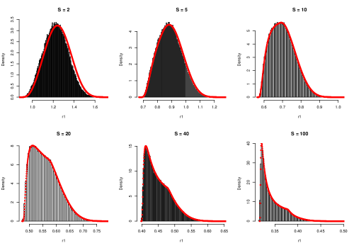
  Figure 1: The normal approximation of (8) compared to a direct simulation from the conditional distribution.

  The approximation compares well with the simulation over different values of $s$.

• Via the transformation in (3), the point of approximation becomes the mean. This allows us to get uniform relative error in the approximation, at the expense of having to compute $\xi(y,r)$.

• The precision of the approximation can be increased arbitrarily, in principle, if we integrate numerically over $r_{i}$, $i=1,\dots,\ell$, and approximate $f_{\overline{S}^{(r_{\ell})}}$. The order of the error improves, if we replace the normal approximation by the Edgeworth expansion of an appropriate order depending on $\ell$.

The next theorem formalizes the above approximation scheme and gives a rigorous error estimate. Fix a number $a_{0}$ such that $0<a_{0}<(d/\gamma)/d_{1}$. Let

$$\begin{split}\mathfrak{f}^{\ell,k}_{R_{1},S}(r_{1},\,s)&:=\int_{r_{1}}^{\infty}dr_{2}\,\cdots\int_{r_{\ell-1}}^{\infty}dr_{\ell}\,f_{R_{1},\dots,R_{\ell}}\left(r_{1},\dots,r_{\ell}\right)\,\mathfrak{g}_{\ell,k}(y,r_{\ell}),\end{split}$$

where

$$\begin{split}\mathfrak{g}_{\ell,k}(y,r)&=\begin{cases}\frac{1}{\sigma(r)}\,\widetilde{\mathfrak{n}}_{k}\,e^{-\xi(y,r)y}\,\varphi_{Y^{(r)}}(-\xi(y,r))&\text{when $r>(a_{0}\,\ell)^{1/d}$;}\\ 0&\text{when $r\leq(a_{0}\,\ell)^{1/d}$}\end{cases}\end{split}$$

and

$$y=y(s,r_{1},\dots,r_{\ell})=\frac{s-r_{1}^{-\gamma}-\dots-r_{\ell}^{-\gamma}-\mu(r_{\ell})}{\sigma(r_{\ell})}.$$

Theorem 2.

There are constants $C_{5},C_{6},c_{1}$ such that when $\ell\geq C_{5}$ and $k=\lfloor\sqrt{a_{0}\,\ell}\rfloor$, then we have

$$\left|\mathbf{P}[R_{1}\leq r\,|\,S=s]-\frac{1}{f_{S}(s)}\,\int_{s^{-1/\gamma}}^{r}\mathfrak{f}^{\ell,k}_{R_{1},S}(r_{1},\,s)\,dr_{1}\right|\leq C_{6}\,e^{-c_{1}\sqrt{\ell}\log\ell},\quad r>s^{-1/\gamma},\,s>0.$$ (9)

Remark 3.

The above theorem applies just as well, if the path-loss function behaves differently in a neighbourhood of $0$, for example, if

$$f(r)=\begin{cases}r^{-\gamma}&\text{when $r>r_{0}$;}\\ r_{0}^{-\gamma}&\text{when $0\leq r\leq r_{0}$,}\end{cases}$$

and $S=\sum_{k}f(R_{k})$. For this case, we merely have to choose $C_{5}$ large relative to $r_{0}$, and change the definition of $y$ to $(s-f(r_{1})-\dots-f(r_{\ell})-\mu(r_{\ell}))/\sigma(r_{\ell})$. In this case, no series expansion would be available to compute $f_{S}(s)$. Instead, the approximation $f_{S}(s)\approx\int_{0}^{\infty}\mathfrak{f}^{\ell,k}_{R_{1},S}(r_{1},\,s)\,dr_{1}$ can be used.

The following stochastic comparison plays a key role in ensuring that the error bound in Theorem 2 is uniform in $s$. Let $(R^{\prime}_{1},R^{\prime}_{2},\dots)$ have the same law as $(R_{1},R_{2},\dots)$.

Theorem 3.

Let $\gamma>d$ and let $0<s<\infty$. There is a coupling between the conditional law of the collection $(R_{1},R_{2},\dots)$ given $S=s$ and the unconditional law of the collection $(R^{\prime}_{1},R^{\prime}_{2},\dots)$, such that a.s. we have $R^{\prime}_{i-1}\leq R_{i}$ for all $i\geq 2$.

1.4 Related works

A lower bound on $R_{1}$ is $S^{-1/\gamma}$, and when $S$ is large, this is a good first approximation. The first term in the right hand side of (1) dominates the sum, in the sense that $R_{1}^{-\gamma}$ has the same tail behaviour as $S$ [15, Section 1.4]. The error of the simple heuristic $R_{1}\approx S^{-1/\gamma}$ for large $S$ is considered in [17, 13].

A more general setup than considered above is to study a random field of the form $S_{f}(x)=\sum_{P}f(P-x)$, $x\in\mathbb{R}^{d}$, where the summation is over points $P$ of the Poisson process (called Poisson shot noise). If $f$ is the function $f_{r}(y)=|y|^{-\gamma}\,\mathbf{1}_{|y|>r}$, then $\overline{S}^{(r)}=S_{f_{r}}(o)$, where $o$ is the origin. Rice [14, Section 1.6] proved that under certain general conditions on $f$, $S_{f}(o)$ approaches a normal law as the Poisson density approaches infinity. It follows from this that $S_{f_{r}}(o)$ is asymptotically normal as $r\to\infty$ (after rescaling the Poisson process so that $r$ becomes $1$). Rice also states the Edgeworth expansion around this normal limit. Lewis [11] gives error estimates (for a slightly modified version) for general $f$ and all orders, with the dependence on $f$ implicit. Explicit error estimates for the normal and Edgeworth approximation of infinitely divisible distributions, inclusing Poisson shot noise, were considered by Lorz and Heinrich [12]. They considered the supremal additive error in approximating the distribution function, with error estimates given in detail for the second order Edgeworth approximation. A novelty of our work is that we provide details of the estimate for all orders, giving the dependence of the error term on the order. By considering the transformed distribution we get very good relative error estimates (the relative error improves away from the mean). All constants in our estimates could be made explicit (with tedious but straightforward arguments), but we refrained from doing so for the sake of readability.

A possible alternative approach to approximating $\overline{S}^{(r)}$ would be to find a suitable series expansion for the density. Feller [6, Section XVII.6] gives a pointwise convergent series for stable densities, and Zolotarev [16] studies their analytical properties in detail. We note that, unlike in the case of the stable random variable $S$, the logarithm of the characteristic function of $\overline{S}^{(r)}$ is no longer given in closed form, which we believe makes it more problematic to derive a useful series. Another alternative would be to generalize the series of Brockwell and Brown [2] using Laguerre polynomials. We believe that the merit of our approach compared to these possibilities is that it is more probabilistic, and that the Edgeworth estimates we develop here are of interest in their own right, and possibly apply to more general infinitely divisible families.

In the context of wireless applications, Baccelli and Biswas [1] consider the joint distribution of the signals measured at a finite number of points (with a more general pathloss function than ours), and show asymptotic independence as the Poisson density approaches infinity. They also consider percolative properties of a random graph defined in terms of signal-to-interference ratios.

The rest of the paper is organized as follows. In Section 2 we collect some preliminary results and define the quantities appearing in Theorem 1. In Section 3 we prove Theorem 1. In Section 4 we prove Theorem 3 and use it to prove Theorem 2 building on the technical estimate of Theorem 1. In Section 5 we show that when $d/\gamma=1/2$ and we take $\ell\geq 4$, one integration over $(r_{1},\dots,r_{\ell})$ can be carried out analytically.

2 Preliminaries

Recall that $R_{1}<R_{2}<\dots$ are the radii of the points of a Poisson process in $\mathbb{R}^{d}$ of intensity $\lambda>0$. It will sometimes be convenient to consider the following finite version: let $R^{(n)}_{1}<\dots<R^{(n)}_{n}$ be the radii of $n$ independent points chosen uniformly at random from the ball of volume $n/\lambda$ centred at the origin.

Recall that $\overline{S}^{(r)}=\sum_{i:R_{i}>r}R_{i}^{-\gamma}$, $r\geq 0$. The following lemma, whose proof follows easily from large deviation bounds for Binomial and Poisson variables, and is left to the reader, implies in particular that the sum defining $\overline{S}^{(r)}$ converges almost surely for all $\gamma>d$, $r\geq 0$.

Lemma 1.

There exist constants $c=c(\lambda,d)$ and $C=C(\lambda,d)$ such that for all $k\geq 0$ and $r\geq 0$, we have

$$\begin{split}\mathbf{P}\left[\#\{j:r+k\leq R^{(n)}_{j}<r+k+1\}\geq C(r+k)^{d-1}\right]&\leq e^{-c(r+k)}\\ \mathbf{P}\left[\#\{j:r+k\leq R_{j}<r+k+1\}\geq C(r+k)^{d-1}\right]&\leq e^{-c(r+k)}.\end{split}$$ (10)

We will need to approximate $S$ by $S^{(n)}:=\sum_{j=1}^{n}\left(R^{(n)}_{j}\right)^{-\gamma}$. The following lemma provides a quantitative estimate on the rate of convergence. An estimate of this type was proved by Cramér [3] (who gave the details in the symmetric stable case). For the sake of being self-contained, we provide a proof in Appendix A.

Lemma 2.

There exist $C=C(\gamma,d)$, $\delta=\delta(\gamma,d)$ such that $\sup_{s\in\mathbb{R}}\left|f_{S^{(n)}}(s)-f_{S}(s)\right|\leq C\,n^{-\delta}$.

Recall that

$$\begin{split}Y^{(r)}&=\frac{\overline{S}^{(r)}-\mu(r)}{\sigma(r)},\qquad\text{where }\mu(r)=\mathbf{E}\left[\overline{S}^{(r)}\right],\quad\sigma^{2}(r)=\mathsf{Var}\left(\overline{S}^{(r)}\right).\end{split}$$

Note that since $\overline{S}^{(r)}>0$ a.s., we have $Y^{(r)}>-\frac{\mu(r)}{\sigma(r)}$ a.s.

Next, we compute the Laplace transforms of $\overline{S}^{(r)}$ and $Y^{(r)}$. Writing $|\mathbf{x}|$ for the Euclidean norm of $\mathbf{x}\in\mathbb{R}^{d}$, and $\omega_{d-1}$ for the measure of the $d-1$-sphere, we have:

$$\begin{split}\varphi_{\overline{S}^{(r)}}(t)&:=\mathbf{E}\left[e^{-t\overline{S}^{(r)}}\right]=\exp\left(\int_{\{\mathbf{x}:|\mathbf{x}|>r\}}\left(e^{-t\,|\mathbf{x}|^{-\gamma}}-1\right)\lambda\,d\mathbf{x}\right)\\ &=\exp\left(\lambda\,\omega_{d-1}\int_{r}^{\infty}q^{d-1}\,\left(e^{-tq^{-\gamma}}-1\right)\,dq\right).\end{split}$$

When $r=0$, this shows that $\varphi_{S}(t)=\exp(-b_{1}\,t^{d/\gamma})$, with $b_{1}(\lambda,\gamma,d)=\frac{\lambda\,\omega_{d-1}}{d}\Gamma(1-d/\gamma)>0$, and hence $S$ has a one-sided stable distribution of index $d/\gamma$ [6, Section XVII.5]. For $r>0$, we change variables via $q=r\,u^{-1/\gamma}$, which gives

$$\begin{split}\varphi_{\overline{S}^{(r)}}(t)&=\exp\left(\frac{\lambda\,\omega_{d-1}}{\gamma}\,r^{d}\,\int_{0}^{1}\left(e^{-r^{-\gamma}tu}-1\right)\,u^{-1-d/\gamma}\,du\right).\end{split}$$

Letting $a_{1}=a_{1}(r)=(\lambda\omega_{d-1}/\gamma)\,r^{d}$, and $a_{2}=a_{2}(r)=r^{-\gamma}$, we can then write

$$\varphi_{\overline{S}^{(r)}}(t)=\exp\left(a_{1}\,\psi(a_{2}t)\right),$$ (11)

where

$$\begin{split}\psi(a_{2}\,t)&=\int_{0}^{1}\left(e^{-a_{2}tu}-1\right)\,u^{-1-d/\gamma}\,du=\sum_{n=1}^{\infty}\frac{(-a_{2})^{n}t^{n}}{n!\,(n-d/\gamma)}.\end{split}$$ (12)

In particular, the mean and variance of $\overline{S}^{(r)}$ are

$$\begin{split}\kappa_{1}=\kappa_{1}(r)=\mu(r)=\frac{a_{1}a_{2}}{1-d/\gamma}\qquad\text{ and }\qquad\kappa_{2}=\kappa_{2}(r)=\sigma^{2}(r)=\frac{a_{1}a_{2}^{2}}{2-d/\gamma},\end{split}$$

and the higher order cumulants are given by

$$\kappa_{n}=\kappa_{n}(r)=\frac{a_{1}a_{2}^{n}}{n-d/\gamma},\quad n\geq 3.$$

Since the value of $\lambda$ can be fixed by scaling, we specialize to $\lambda=(2\gamma-d)/\omega_{d-1}$, which yields the simple form $\sigma(r)=r^{\frac{d}{2}-\gamma}$. Letting $d_{1}=d_{1}(d,\gamma):=2-\frac{d}{\gamma}$, and recalling the notation $\rho=r^{d/2}$, we can write $\varphi_{Y^{(r)}}(t)$ in the form:

$$\begin{split}\varphi_{Y^{(r)}}(t)&=\exp\left(d_{1}\,r^{d}\,\psi_{0}\left(\frac{t}{r^{d/2}}\right)\right)=\exp\left(d_{1}\,\rho^{2}\,\psi_{0}\left(\frac{t}{\rho}\right)\right)\qquad\text{where}\\ \psi_{0}(s)&:=\int_{0}^{1}(e^{-su}-1-su)\,u^{-1-d/\gamma}\,du=\sum_{n=2}^{\infty}\frac{(-s)^{n}}{n!\,(n-\frac{d}{\gamma})}.\end{split}$$ (13)

We now collect some estimates for the characteristic function of $Y^{(r)}$. From (13) we have that the Fourier transform of $Y^{(r)}$ is given by

$$\begin{split}\chi_{Y^{(r)}}(t)&=\exp\left(-\frac{t^{2}}{2}+\sum_{n=3}^{\infty}\kappa^{\prime}_{n}(r)\frac{(it)^{n}}{n!}\right)=\exp\left(d_{1}\,r^{d}\,\sum_{n=2}^{\infty}\frac{(it/r^{d/2})^{n}}{(n-d/\gamma)\,n!}\right)\\ &=\exp\left(d_{1}\,r^{d}\,\int_{0}^{1}\left(e^{itu/r^{d/2}}-1-\frac{itu}{r^{d/2}}\right)\,u^{-1-d/\gamma}\,du\right)=\left(\chi_{Y^{(1)}}(t/r^{d/2})\right)^{r^{d}},\end{split}$$ (14)

where $\kappa^{\prime}_{n}(r)$ are the cumulants of $Y^{(r)}$.

We will need estimates on $\chi_{Y^{(r)}}$ away from the real axis.

Lemma 3.

(i) For any $\xi>0$ we have

$$\left|\chi_{Y^{(r)}}(t-i\xi)\right|\leq\varphi_{Y^{(r)}}(-\xi)\,\left|\chi_{Y^{(r)}}(t)\right|.$$

(ii) For any $\zeta>0$ we have

$$\left|\chi_{Y^{(r)}}(t+i\zeta)\right|\leq\varphi_{Y^{(r)}}(\zeta)\,\left|\chi_{Y^{(r)}}(t)\right|^{e^{-\zeta/r}}.$$

(iii) For any $\xi,\zeta>0$ we have

$$\lim_{|t|\to\infty}\,\sup_{-\zeta\leq\mu\leq\xi}\,\left|\chi_{Y^{(r)}}(t-i\mu)\right|=0.$$

Proof.

For any $\xi\in\mathbb{R}$ we have

$$\begin{split}&\mathfrak{Re}\log\chi_{Y^{(r)}}(t-i\xi)\\ &\quad=d_{1}\,r^{d}\,\mathfrak{Re}\int_{0}^{1}\left(e^{(itu+\xi u)/r^{d/2}}-1-\frac{itu+\xi u}{r^{d/2}}\right)u^{-1-d/\gamma}\,du\\ &\quad=d_{1}\,r^{d}\,\int_{0}^{1}e^{\xi u/r^{d/2}}\left(\cos\left(\frac{tu}{r^{d/2}}\right)-1\right)u^{-1-d/\gamma}\,du+\int_{0}^{1}\left(e^{\xi u/r^{d/2}}-\frac{\xi u}{r^{d/2}}-1\right)u^{1-d/\gamma}\,du\\ &\quad\leq\min\left\{e^{\xi/r^{d/2}},1\right\}\,d_{1}\,r^{d}\,\int_{0}^{1}\left(\cos\left(\frac{tu}{r^{d/2}}\right)-1\right)\,u^{-1-d/\gamma}\,du+\log\varphi_{Y^{(r)}}(-\xi)\\ &\quad=\min\left\{e^{\xi/r^{d/2}},1\right\}\,\mathfrak{Re}\log\chi_{Y^{(r)}}(t)+\log\varphi_{Y^{(r)}}(-\xi).\end{split}$$ (15)

When $\xi>0$, we obtain (i) immediately, and statement (ii) follows by taking $\xi=-\zeta$. Statement (iii) follows from (i), (ii) and the facts that $\lim_{|t|\to\infty}|\chi_{Y^{(r)}}(t)|=0$, and $\sup_{-\zeta\leq\mu\leq\xi}\varphi_{Y^{(r)}}(-\mu)<\infty$. ∎

In order to approximate $f_{Y^{(r)}}(y)$ for a given $y$, we consider $\widetilde{Y}^{(r)}$ introduced in (3). Recall the expression:

$$\begin{split}f_{\widetilde{Y}^{(r)}}(z)&=\frac{e^{\xi(y,r)z}}{\varphi_{Y^{(r)}}(-\xi(y,r))}f_{Y^{(r)}}(z),\quad z\in\mathbb{R}.\end{split}$$

The parameter $\xi=\xi(y,r)$ is the solution to the equation

$$\frac{y}{\rho}=-d_{1}\,\psi_{0}^{\prime}(-\xi/\rho)=d_{1}\,\sum_{n=2}^{\infty}\frac{(\xi/\rho)^{n-1}}{(n-1)!\,(n-\frac{d}{\gamma})}.$$ (16)

From the definition of $\widetilde{Y}^{(r)}$, we have that the mean and higher order cumulants of $\widetilde{Y}^{(r)}$ are $y$ and $\widetilde{\kappa}_{n}/\rho^{n-2}$, where

$$\begin{split}\mathbf{E}[\widetilde{Y}^{(r)}]=y\qquad\text{ and }\qquad\widetilde{\kappa}_{n}:=d_{1}\,\int_{0}^{1}e^{\xi u/r^{d/2}}\,u^{n-1-d/\gamma}\,du,\quad n\geq 2,\end{split}$$ (17)

We have the following relationship between $\chi_{Y^{(r)}}$ and $\chi_{\widetilde{Y}^{(r)}}$:

$$\chi_{Y^{(r)}}(t-i\xi)=\varphi_{Y^{(r)}}(-\xi)\int_{-\infty}^{\infty}e^{itz}\frac{e^{\xi z}}{\varphi_{Y^{(r)}}(-\xi)}f_{Y^{(r)}}(z)\,dz=\varphi_{Y^{(r)}}(-\xi)\chi_{\widetilde{Y}^{(r)}}(t).$$ (18)

From this we obtain

$$\begin{split}f_{Y^{(r)}}(y)&=\frac{1}{2\pi}\int_{-\infty}^{\infty}e^{-ity}\,\chi_{Y^{(r)}}(t)\,dt=\frac{1}{2\pi}\int_{-\infty}^{\infty}e^{-ity-\xi y}\,\chi_{Y^{(r)}}(t-i\xi)\,dt\\ &=\frac{e^{-\xi y}\varphi_{Y^{(r)}}(-\xi)}{2\pi}\int_{-\infty}^{\infty}e^{-ity}\,\chi_{\widetilde{Y}^{(r)}}(t)\,dt.\end{split}$$ (19)

In the second step we moved the path of integration, which is justified by Lemma 3(iii). Our goal will be to estimate the expression

$$\begin{split}e^{-ity}\,\chi_{\widetilde{Y}^{(r)}}(t)=\exp\left(d_{1}\,\rho^{2}\,\int_{0}^{1}e^{\xi u/\rho}\left(e^{itu/\rho}-1-\frac{itu}{\rho}\right)\,u^{-1-d/\gamma}\,du\right).\end{split}$$ (20)

Recall $\widetilde{\kappa}_{k}$ defined in (17):

$$\widetilde{\kappa}_{k}=d_{1}\,\int_{0}^{1}e^{\xi u/\rho}\,u^{k-1-d/\gamma}\,du,\quad k\geq 2.$$ (21)

It is clear from this formula that with $d_{3}=d_{1}/(1-\frac{d}{\gamma})$, for all $-d_{3}\,\rho<y<\infty$ we have $\widetilde{\kappa}_{2}\geq\widetilde{\kappa}_{3}\geq\dots>0$.

Remark 4.

Let us comment on how the approximation in Theorem 1 can be computed numerically. The functional relationship between $y/\rho$ and $\xi/\rho$ does not depend on $r$, and is found to be

$$\frac{y}{\rho}=d_{1}\,\int_{0}^{1}\left(e^{\xi u/\rho}-1\right)\,u^{-d/\gamma}.$$

The right hand side can be written in terms of the regularized incomplete gamma function, for which efficient numerical evaluation is available both for positive arguments (when $\xi<0$, equivalently, $y<0$) [7]; and for negative argumments (when $\xi>0$, equivalently, $y>0$) [8]. Thus the increasing convex function $(\xi/\rho)\mapsto(y/\rho)$ can be easily inverted using Newton’s method. The expression $e^{-\xi y}\,\varphi_{Y^{(r)}}(-\xi)$ can be written in the form $\exp(\rho^{2}\,h(\xi/\rho,y/\rho))$ with an explicit function $h$. The number $\widetilde{\kappa}_{2}$ as well as all $\widetilde{\kappa}_{n}$’s, are again given in terms of incomplete gamma functions.

As mentioned earlier, for large $r$, the order of the approximation can be improved, if we replace the normal approximation by an Edgeworth expansion [6, Section XVI], and we are now ready to define the quantities appearing in Theorem 1. A reader not familiar with the expansion should note that it is possible to follow our proof of Theorem 1 without prior exposure, as it is self-contained. On the other hand, the somewhat complicated expressions one needs to define (see (22) and (23) below) may become more transparent upon reading [6, Section XVI].

Recall that $\mathfrak{n}$ denotes the standard normal density, and for $k=0$ define

$$\widetilde{\mathfrak{n}}_{0}:=\frac{1}{\sqrt{\widetilde{\kappa}_{2}}}\,\mathfrak{n}(0).$$

For $k\geq 1$, and $j\geq 1$, $1\leq\ell\leq j$ define

$$\widetilde{c}_{j,\ell}=\frac{1}{\ell!}\!\!\!\!\!\sum_{\begin{subarray}{c}3\leq n_{1},\dots,n_{\ell}\leq k+2\\ (n_{1}-2)+\dots+(n_{\ell}-2)=j\end{subarray}}\frac{\widetilde{\kappa}_{n_{1}}}{n_{1}!}\cdots\frac{\widetilde{\kappa}_{n_{\ell}}}{n_{\ell}!}.$$ (22)

Let

$$\begin{split}\widetilde{\mathfrak{n}}_{k}:=\frac{1}{\sqrt{\widetilde{\kappa}_{2}}}\mathfrak{n}(0)\left[1+\sum_{j=1}^{k}\frac{(-1)^{j}}{(r^{d/2})^{j}}\,\sum_{\ell=1}^{j}\,\frac{\widetilde{c}_{j,\ell}}{\widetilde{\kappa}_{2}^{\frac{j}{2}+\ell}}\,H_{j+2\ell}(0)\right],\quad k\geq 1,\end{split}$$ (23)

where $H_{n}(z)$, $n\geq 0$, denotes the $n$-th Hermite polynomial, that is, $(-1)^{n}H_{n}(z)\mathfrak{n}(z)$ has Fourier transform $(it)^{n}\,e^{-t^{2}/2}$. Observe that in computing $\widetilde{\mathfrak{n}}_{k}(0)$, all terms with odd $j$ vanish. In particular, $\widetilde{\mathfrak{n}}_{2k+1}=\widetilde{\mathfrak{n}}_{2k}$ for $k=0,1,\dots$.

We close this section with collecting a few estimates that we will often use. We have [6, Eqn. XVI.(2.8)]:

$$\left|e^{\alpha}-e^{\beta}\right|\leq e^{-x}\left|\alpha-\beta\right|\,\exp\left(\max\{|\alpha+x|,\,|\beta+x|\}\right),\quad\alpha,\beta\in\mathbb{C},\,x\in\mathbb{R}.$$ (24)

The following estimate is standard for the tail of the normal distribution (see for example [4, Theorem (1.4)]):

$$\int_{x}^{\infty}\exp(-t^{2}a/2)\,dt\leq\frac{1}{a\,x}\,\exp(-x^{2}a/2).$$ (25)

We will use the following Gaussian absolute moments:

$$\int_{-\infty}^{\infty}|t|^{k}\,\exp(-t^{2}a/2)\,dt=\left(\frac{2}{a}\right)^{\frac{k+1}{2}}\,\Gamma\left(\frac{k+1}{2}\right).$$ (26)

3 Estimates of the transformed distribution

In this section we prove Theorem 1. The arguments for $k=0$ (normal approximation) are similar and simpler than for $k\geq 1$. Therefore, we only give the details when $k\geq 1$.

We will often use Stirling’s formula [5, Section II.9] in the form:

$$\sqrt{2\pi N}N^{N}e^{-N}\leq\Gamma(N+1)\leq\sqrt{2\pi N}N^{N}e^{-N+\frac{1}{12N}},\qquad N\geq 1.$$ (27)

3.1 Upper tail

In this section we prove Theorem 1 in the case $y\geq 0$. It follows then from the definition of $\xi=\xi(y,r)$ that $0\leq\xi(y,r)<\infty$, and from (21) that $\widetilde{\kappa}_{2}\geq 1$. Recall that $\rho=r^{d/2}$. Recall the formula (19) and that our goal is to approximate

$$\begin{split}e^{-ity}\,\chi_{\widetilde{Y}^{(r)}}(t)=\exp\left(d_{1}\,\rho^{2}\,\int_{0}^{1}e^{\xi u/\rho}\left(e^{itu/\rho}-1-\frac{itu}{\rho}\right)\,u^{-1-d/\gamma}\,du\right)=:e^{u(t)}.\end{split}$$ (28)

We define

$${q}_{k}(t) =\rho^{2}\,\sum_{n=3}^{k+2}\frac{(it/\rho)^{n}\,\widetilde{\kappa}_{n}}{n!} {r}_{k}(t) =\rho^{2}\,\sum_{n=k+3}^{\infty}\frac{(it/\rho)^{n}\,\widetilde{\kappa}_{n}}{n!}$$ (29)

$${u}(t) =-\frac{t^{2}}{2}\widetilde{\kappa}_{2}+{q}_{k}(t)+{r}_{k}(t) {\widetilde{\chi}}_{k}(t) :=\exp\left(-\frac{t^{2}}{2}\widetilde{\kappa}_{2}+{q}_{k}(t)\right).$$ (30)

We give separate estimates for $|t|\leq\rho/2$ and $|t|>\rho/2$. For $|t|\leq\rho/2$, we estimate $e^{-ity}\,\chi_{\widetilde{Y}^{(r)}}(t)=e^{{u}(t)}$ first by ${\widetilde{\chi}}_{k}(t)=\exp\left(-\frac{t^{2}}{2}\,\widetilde{\kappa}_{2}+{q}_{k}(t)\right)$, then by the Taylor expansion of $e^{{q}_{k}(t)}$. Keeping terms of order $\rho^{-k}$ and lower yields the Edgeworth expansion. The above steps are carried out in a series of lemmas.

Lemma 4.

There exists a constant $C$ such that for all $r\geq 1$ and $k\geq 1$ we have

$$\begin{split}\int_{-\rho/2}^{\rho/2}\left|e^{{u}(t)}-{\widetilde{\chi}}_{k}(t)\right|\,dt\leq\frac{1}{\sqrt{\widetilde{\kappa}_{2}}}\,\frac{C^{k}\,k^{-\frac{k}{2}}}{(\sqrt{\widetilde{\kappa}_{2}}\,\rho)^{k+1}}.\end{split}$$

Proof.

Let $\alpha(t)=-\frac{t^{2}\,\widetilde{\kappa}_{2}}{2}+q_{k}(t)$, $\beta(t)=u(t)$ and $x(t)=\frac{t^{2}\,\widetilde{\kappa}_{2}}{2}$. For all $t\in\mathbb{R}$, $0\leq u\leq 1$, $r\geq 1$ and $k\geq 1$ we have

$$\begin{split}\left|\left(e^{itu/\rho}-1-\frac{itu}{\rho}\right)-\left(\sum_{n=2}^{k+2}\frac{(itu)^{n}}{\rho^{n}\,n!}\right)\right|\leq\frac{|t|^{k+3}\,u^{k+3}}{\rho^{k+3}\,(k+3)!}.\end{split}$$

Multiplying by $d_{1}\,\rho^{2}\,e^{\xi u/\rho}u^{-1-d/\gamma}$, integrating over $0\leq u\leq 1$, and using Stirling’s formula yields that for $|t|\leq\rho/2$, we have

$$\begin{split}\left|\beta(t)-\alpha(t)\right|\leq t^{2}\,\frac{|t|^{k+1}}{\rho^{k+1}\,(k+3)!}\,\widetilde{\kappa}_{k+3}.\end{split}$$

We also have

$$\begin{split}&\max\{|\alpha(t)+x(t)|,\,|\beta(t)+x(t)|\}=\max\{|q_{k}(t)|,\,|q_{k}(t)+r_{k}(t)|\}\leq\rho^{2}\,\sum_{n=3}^{\infty}\frac{|t|^{n}\,\widetilde{\kappa}_{n}}{\rho^{n}\,n!}\\ &\qquad\leq\frac{|t|^{3}}{\rho}\,\widetilde{\kappa}_{3}\,\sum_{n=3}^{\infty}\frac{|t|^{n-3}}{\rho^{n-3}\,(n-3)!\,6}\leq\frac{t^{2}}{2}\,\widetilde{\kappa}_{2}\,\frac{|t|}{3\,\rho}\,e^{|t|/\rho}\leq\frac{t^{2}}{4}\,\widetilde{\kappa}_{2}.\end{split}$$ (31)

Using (24) and then (26) and Stirling’s formula (27) yields:

$$\begin{split}\int_{-\rho/2}^{\rho/2}\left|\chi_{\widetilde{Y}^{(r)}}(t)-{\widetilde{\chi}}_{k}(t)\right|\,dt&\leq\frac{\widetilde{\kappa}_{k+3}}{\rho^{k+1}\,(k+3)!}\,\int_{-\infty}^{\infty}|t|^{k+3}\,e^{-t^{2}\widetilde{\kappa}_{2}/4}\,dt\leq\frac{C^{k}\,k^{-k/2}}{\rho^{k+1}\,\widetilde{\kappa}_{2}^{\frac{k}{2}+1}}.\end{split}$$

∎

Consider now ${\widetilde{\chi}}_{k}(t)=\exp(-\frac{t^{2}}{2}\widetilde{\kappa}_{2}+{q}_{k}(t))$. Expand $e^{{q}_{k}(t)}$ using the exponential power series, and collect terms according to inverse powers of $\rho$. This yields unique polynomials ${p}_{1},{p}_{2},\dots$ with real coefficients, such that

$${\widetilde{\chi}}_{k}(t)=e^{-t^{2}\widetilde{\kappa}_{2}/2}\,\left[1+\sum_{j=1}^{k}\frac{{p}_{j}(it)}{\rho^{j}}+{\tilde{r}}_{k}(t)\right]=\chi_{k}(t)+e^{-t^{2}\widetilde{\kappa}_{2}/2}{\tilde{r}}_{k}(t),$$ (32)

where ${\tilde{r}}_{k}$ collects all the terms of order $\rho^{-(k+1)}$ and higher, and $\chi_{k}(t)$ is defined by the second equality. More explicitly, recalling (22), we have

$${p}_{j}(it) =\sum_{\ell=0}^{j}\widetilde{c}_{j,\ell}\,(it)^{j+2\ell}.$$

Recall that the main term for the approximation is $\tilde{\mathfrak{n}}_{k}=\frac{1}{2\pi}\int_{-\infty}^{\infty}\chi_{k}(t)\,dt$. The following simple upper bound will be useful.

Lemma 5.

We have

$$\widetilde{c}_{j,\ell}\leq\frac{\left(\widetilde{\kappa}_{3}\right)^{\ell}\,\ell^{j}}{\ell!\,j!}.$$

Proof.

Recalling the definition from (22) we have

$$\begin{split}\widetilde{c}_{j,\ell}&=\frac{1}{\ell!}\sum_{\begin{subarray}{c}3\leq n_{1},\dots,n_{\ell}\leq k+2:\\ (n_{1}-2)+\dots+(n_{\ell}-2)=j\end{subarray}}\frac{\widetilde{\kappa}_{n_{1}}\,\cdots\,\widetilde{\kappa}_{n_{\ell}}}{n_{1}!\cdots n_{\ell}!}\leq\frac{\left(\widetilde{\kappa}_{3}\right)^{\ell}}{\ell!\,j!}\sum_{\begin{subarray}{c}1\leq m_{1},\dots,m_{\ell}\leq k:\\ m_{1}+\dots+m_{\ell}=j\end{subarray}}\frac{j!}{m_{1}!\cdots m_{\ell}!}\leq\frac{\left(\widetilde{\kappa}_{3}\right)^{\ell}\,\ell^{j}}{\ell!\,j!}.\end{split}$$ (33)

∎

We now find an estimate for the error resulting from omitting ${\tilde{r}}_{k}(t)$ in (32). We do this in two steps, summarized in the following two lemmas.

Lemma 6.

There exists a constant $C$ such that for all $r\geq 1$ and $k\geq 1$ we have

$$\int_{-\rho/2}^{\rho/2}e^{-t^{2}\widetilde{\kappa}_{2}/2}\,\left|e^{{q}_{k}(t)}-\sum_{\ell=0}^{k}\frac{{q}_{k}(t)^{\ell}}{\ell!}\right|\,dt\leq\frac{C^{k}\,k^{k/2}}{\sqrt{\widetilde{\kappa}_{2}}\,(\sqrt{\widetilde{\kappa}_{2}}\rho)^{k+1}}.$$ (34)

Proof.

Recalling (LABEL:e:max-qk-rk) we have

$$\left|{q}_{k}(t)\right|\leq\frac{|t|^{3}\,e^{|t|/\rho}}{6\,\rho}\,\widetilde{\kappa}_{2}\leq\frac{t^{2}}{4}\,\widetilde{\kappa}_{2}.$$

Hence the expression inside absolute values in the left hand side of (34) is at most

$$\begin{split}\frac{\left|{q}_{k}(t)\right|^{k+1}}{(k+1)!}\,e^{|{q}_{k}(t)|}&\leq\frac{\widetilde{\kappa}_{2}^{k+1}}{\rho^{k+1}}\,\frac{|t|^{3(k+1)}}{(k+1)!}\,\left(\frac{e^{1/2}}{6}\right)^{k+1}\,e^{t^{2}\widetilde{\kappa}_{2}/4}\leq\frac{C^{k}\,\widetilde{\kappa}_{2}^{k+1}}{\rho^{k+1}}\,\frac{1}{k^{k}}\,|t|^{3(k+1)}\,e^{t^{2}\widetilde{\kappa}_{2}/4}.\end{split}$$ (35)

Using (26) and Stirling’s formula, we have

$$\int_{-\rho/2}^{\rho/2}|t|^{3(k+1)}e^{-t^{2}\widetilde{\kappa}_{2}/4}\,dt\leq\left(\frac{4}{\widetilde{\kappa}_{2}}\right)^{\frac{3}{2}k+2}\,\Gamma\left(\frac{3}{2}k+2\right)\leq C^{k}\,k^{3k/2}\,\widetilde{\kappa}_{2}^{-\frac{3}{2}k-2}.$$

Taking into account the additional terms in the right hand side of (35), this implies that the left hand side of (34) is bounded by the expression claimed in the Lemma. ∎

Lemma 7.

(i) There exists a constant $C$ such that for any $k\geq 1$ and $r\geq 1$ we have

$$\int_{-\rho/2}^{\rho/2}e^{-\frac{t^{2}}{2}\widetilde{\kappa}_{2}}\,\left|1+\sum_{j=1}^{k}\frac{{p}_{j}(it)}{\rho^{j}}-\sum_{\ell=0}^{k}\frac{{q}_{k}(t)^{\ell}}{\ell!}\right|\leq\frac{C^{k}}{\sqrt{\widetilde{\kappa}_{2}}}\,\sum_{j=k+1}^{k^{2}}\frac{k^{j/2}}{(\sqrt{\widetilde{\kappa}_{2}}\rho)^{j}}.$$ (36)

(ii) When $\rho\geq\sqrt{k}$, the right hand side of (36) is at most $\frac{C^{k}\,k^{k/2}}{\sqrt{\widetilde{\kappa}_{2}}(\sqrt{\widetilde{\kappa}_{2}}\rho)^{k+1}}$.

Proof.

(i) We first note that the statement is vacuous when $k=1$, as the expression inside absolute values vanishes then. Henceforth we assume $k\geq 2$. The expression inside absolute values in the left hand side of (36) consists of those terms of $\sum_{\ell}{q}_{k}^{\ell}/\ell!$ where $\rho^{-1}$ occurs with a power at least $k+1$. These are

$$\begin{split}&\sum_{j=k+1}^{k^{2}}\frac{1}{\rho^{j}}\sum_{\ell=\lceil j/k\rceil}^{k}\widetilde{c}_{j,\ell}(it)^{j+2\ell}.\end{split}$$ (37)

For fixed $j$ and $k$, we take absolute values in (LABEL:e:the-terms), and integrate. Formula (26) gives

$$\int_{-\rho/2}^{\rho/2}e^{-\frac{t^{2}}{2}\widetilde{\kappa}_{2}}\,|t|^{j+2\ell}\,dt\leq\left(\frac{2}{\widetilde{\kappa}_{2}}\right)^{\frac{j}{2}+\ell+\frac{1}{2}}\,\Gamma\left(\frac{j}{2}+\ell+\frac{1}{2}\right).$$

Using Lemma 5 to bound $\widetilde{c}_{j,\ell}$, this yields the following bound on the left hand side of (36):

$$\begin{split}&\frac{1}{\sqrt{\widetilde{\kappa}_{2}}}\,\sum_{j=k+1}^{k^{2}}\frac{1}{(\sqrt{\widetilde{\kappa}_{2}}\rho)^{j}}\,\sum_{\ell=\lceil j/k\rceil}^{k}\frac{\ell^{j}\,2^{\frac{j}{2}+\ell+\frac{1}{2}}\,\Gamma(\frac{j}{2}+\ell+\frac{1}{2})}{\ell!\,j!},\end{split}$$ (38)

Fix $k+1\leq j\leq k^{2}$, and consider the ratio of the terms corresponding to $\ell+1$ and $\ell$ in the second sum. This ratio is

$$\begin{split}\frac{(\ell+1)^{j}}{\ell^{j}}\,\frac{2\,(\frac{j}{2}+\ell+\frac{1}{2})}{(\ell+1)}>1.\end{split}$$ (39)

Thus the sum over $\ell$ is bounded above by $k$ times the $\ell=k$ term. This gives

$$\begin{split}&\sum_{\ell=\lceil j/k\rceil}^{k}\frac{\ell^{j}\,2^{\frac{j}{2}+\ell+\frac{1}{2}}\,\Gamma(\frac{j}{2}+\ell+\frac{1}{2})}{\ell!\,j!}\leq k\,\frac{k^{j}\,2^{\frac{j}{2}+k+\frac{1}{2}}\,\Gamma(\frac{j}{2}+k+\frac{1}{2})}{k!\,j!}\\ &\qquad\leq C^{k}\,\frac{k^{j}\,2^{\frac{j}{2}+k}\,\left(\frac{j}{2}+k\right)^{\frac{j}{2}+k}\,e^{-\frac{j}{2}-k}}{k^{k}\,j^{j}\,e^{-j}}\leq C^{k}\,\frac{k^{j}\,\left(j+2k\right)^{\frac{j}{2}+k}\,e^{\frac{j}{2}}}{k^{k}\,j^{j}}.\end{split}$$ (40)

Writing $j=xk$, with $x>1$, the right hand side of (LABEL:e:sum-ell-only) is

$$\begin{split}&C^{k}\,k^{j/2}\,\frac{k^{\frac{x}{2}k}\,\left((2+x)k\right)^{(\frac{x}{2}+1)k}\,e^{\frac{x}{2}k}}{k^{k}\,(xk)^{xk}}=C^{k}\,k^{j/2}\,\frac{(2+x)^{(\frac{x}{2}+1)k}\,e^{\frac{x}{2}k}}{x^{xk}}\\ &\qquad=C^{k}\,k^{j/2}\,\left[\frac{(2+x)^{(\frac{x}{2}+1)}\,e^{\frac{x}{2}}}{x^{x}}\right]^{k}\leq C^{k}\,k^{j/2}.\end{split}$$ (41)

This proves statement (i) of the lemma.

(ii) When $\rho\geq\sqrt{k}$, using $\widetilde{\kappa}_{2}\geq 1$ (which holds due to $y\geq 0$), we have

$$\begin{split}\frac{C^{k}}{\sqrt{\widetilde{\kappa}_{2}}}\,\sum_{j=k+1}^{k^{2}}\frac{k^{j/2}}{(\sqrt{\widetilde{\kappa}_{2}}\,\rho)^{j}}&\leq\frac{C^{k}\,k^{k/2}}{\sqrt{\widetilde{\kappa}_{2}}\,(\sqrt{\widetilde{\kappa}_{2}}\,\rho)^{k+1}}\,\sum_{j=k+1}^{k^{2}}\frac{k^{(j-k)/2}}{\rho^{j-k-1}}\leq\frac{C^{k}\,k^{k/2}}{\sqrt{\widetilde{\kappa}_{2}}\,(\sqrt{\widetilde{\kappa}_{2}}\,\rho)^{k+1}}.\end{split}$$

∎

We also need bounds on the tails of $\chi_{k}(t)$ and $\chi_{\widetilde{Y}^{(r)}}(t)$, in the range $|t|>\frac{1}{2}\rho$.

Lemma 8.

For $|t|>\rho/2$ we have

$$\left|e^{-ity}\,\chi_{\widetilde{Y}^{(r)}}(t)\right|\leq\exp\left(-c\,\rho^{d_{1}}\,|t|^{d/\gamma}\right)\,\exp\left(-c\,\rho^{2}\,\sqrt{\widetilde{\kappa}_{2}}\right).$$ (42)

Proof.

We have

$$\begin{split}\mathfrak{Re}\,\log\left(e^{-ity}\,\chi_{\widetilde{Y}^{(r)}}(t)\right)&=d_{1}\,\rho^{2}\,\int_{0}^{1}e^{\xi u/\rho}\,\left(\cos\left(\frac{tu}{\rho}\right)-1\right)\,u^{-1-d/\gamma}\,du.\end{split}$$ (43)

When $0\leq u\leq\frac{1}{4}\rho\,|t|^{-1}$, we have $|tu/\rho|\leq\frac{1}{4}$, and $\cos(tu/\rho)\leq 1-t^{2}u^{2}/4\rho^{2}$. Therefore, the contribution of this interval of $u$ to the right hand side of (43) is at most

$$\begin{split}&-d_{1}\,\rho^{2}\,\int_{0}^{\frac{1}{4}\rho|t|^{-1}}\frac{t^{2}u^{2}}{4\rho^{2}}\,u^{-1-d/\gamma}\,du=-\frac{t^{2}}{4}\,d_{1}\,\int_{0}^{\frac{1}{4}\rho|t|^{-1}}u^{1-d/\gamma}\,du\\ &\qquad=-\frac{t^{2}}{4}\,d_{1}\,\left(\frac{1}{4}\right)^{d_{1}}\,\rho^{d_{1}}\,|t|^{-d_{1}}=-c\,\rho^{d_{1}}\,|t|^{d/\gamma}.\end{split}$$ (44)

On the other hand, the contribution of the interval $1/2\leq u\leq 1$ to the right hand side of (43) is at most

$$\begin{split}d_{1}\,\rho^{2}\,\sqrt{e^{\xi/\rho}}\,2^{1+d/\gamma}\,\int_{1/2}^{1}\left(\cos\left(\frac{tu}{\rho}\right)-1\right)\,du\leq-c\,\rho^{2}\,\sqrt{e^{\xi/\rho}}.\end{split}$$ (45)

In the last step we used that the period of the cosine function inside the integral is $O(1)$, and hence the value of the integral is bounded above by a negative constant independent of $r$ and $t$. Moreover, we have

$$\begin{split}\widetilde{\kappa}_{2}=d_{1}\,\int_{0}^{1}e^{\xi u/\rho}\,u^{1-d/\gamma}\,du\leq e^{\xi/\rho},\end{split}$$ (46)

which implies that the right hand side of (45) is at most $-c\,\rho^{2}\,\sqrt{\widetilde{\kappa}_{2}}$. Combining (LABEL:e:decaying), (45) and (46) yields the statement of the lemma. ∎

Lemma 9.

Suppose $\rho\geq\sqrt{k}$. Then we have

$$\int_{|t|>\rho/2}|\chi_{k}(t)|\,dt\leq\frac{C^{k}\,k^{k/2}}{\sqrt{\widetilde{\kappa}_{2}}\,(\sqrt{\widetilde{\kappa}_{2}}\rho)^{k+1}}\quad\text{ and }\quad\int_{|t|>\rho/2}\left|\chi_{\widetilde{Y}^{(r)}}(t)\right|\,dt\leq\frac{C^{k}\,k^{k/2}}{\sqrt{\widetilde{\kappa}_{2}}\,(\sqrt{\widetilde{\kappa}_{2}}\rho)^{k+1}}.$$

Proof.

Using Lemma 5, the integral in the first claim can be estimated by

$$\begin{split}\int_{|t|>\rho/2}|\chi_{k}(t)|\,dt&\leq 2\int_{\rho/2}^{\infty}e^{-\frac{t^{2}}{2}\widetilde{\kappa}_{2}}\left[1+\sum_{j=1}^{k}\frac{\left|{p}_{j}(it)\right|}{\rho^{j}}\right]\,dt\\ &\leq\frac{C}{\widetilde{\kappa}_{2}\,\rho}e^{-\rho^{2}\widetilde{\kappa}_{2}/8}+2\sum_{j=1}^{k}\frac{1}{\rho^{j}}\sum_{\ell=1}^{j}\frac{\left(\widetilde{\kappa}_{2}\right)^{\ell}\,\ell^{j}}{\ell!\,j!}\int_{\rho/2}^{\infty}t^{j+2\ell}\,e^{-\frac{t^{2}}{2}\widetilde{\kappa}_{2}}\,dt.\end{split}$$ (47)

Repeated integration by parts yields

$$\begin{split}\int_{\rho/2}^{\infty}t^{j+2\ell}\,e^{-\frac{t^{2}}{2}\widetilde{\kappa}_{2}}\,dt=\frac{2\,e^{-\rho^{2}\widetilde{\kappa}_{2}/8}}{\widetilde{\kappa}_{2}\,\rho}\,\left[\left(\rho/2\right)^{j+2\ell}+\frac{(j+2\ell-1)}{\widetilde{\kappa}_{2}}\,\left(\rho/2\right)^{j+2\ell-3}+\dots\right].\end{split}$$

Since $j+2\ell-1\leq 3k-1\leq 3\,\rho^{2}=12\,(\rho/2)^{2}$ and $\widetilde{\kappa}_{2}\geq 1$, the right hand side is bounded above by

$$\frac{C\,e^{-\rho^{2}\widetilde{\kappa}_{2}/8}}{\widetilde{\kappa}_{2}\,\rho}\,3k\,\left(\rho/2\right)^{j+2\ell}\leq\frac{C^{k}\,e^{-\rho^{2}\widetilde{\kappa}_{2}/8}}{\widetilde{\kappa}_{2}\,\rho}\,\frac{\rho^{j+2\ell}}{16^{j}}.$$

Substituting this into the right hand side of (47), we get the upper bound

$$\begin{split}\frac{e^{-\rho^{2}\widetilde{\kappa}_{2}/8}}{\widetilde{\kappa}_{2}\,\rho}\,\left[2+C^{k}\,\sum_{j=1}^{k}\frac{1}{16^{j}\,j!}\sum_{\ell=1}^{j}\frac{\left(\widetilde{\kappa}_{2}\,\rho^{2}\right)^{\ell}\,\ell^{j}}{\ell!}\right].\end{split}$$

Since $\widetilde{\kappa}_{2}\,\rho^{2}\geq k$, in the second sum the last term is the largest, and hence we have the bound:

$$\begin{split}\frac{e^{-\rho^{2}\widetilde{\kappa}_{2}/8}}{\widetilde{\kappa}_{2}\,\rho}\,\left[2+C^{k}\,\sum_{j=1}^{k}\frac{(\widetilde{\kappa}_{2}\,\rho^{2})^{j}}{16^{j}\,j!}\right]\leq\frac{e^{-\rho^{2}\widetilde{\kappa}_{2}/8}}{\widetilde{\kappa}_{2}\,\rho}\,\left[2+C^{k}\,e^{\rho^{2}\,\widetilde{\kappa}_{2}/16}\right]\leq\frac{C^{k}\,e^{-\rho^{2}\widetilde{\kappa}_{2}/16}}{\widetilde{\kappa}_{2}\,\rho}.\end{split}$$

The last expression equals

$$\begin{split}\frac{C^{k}\,k^{k/2}}{\sqrt{\widetilde{\kappa}_{2}}\,(\sqrt{\widetilde{\kappa}_{2}}\rho)^{k+1}}\,\exp\left(-\frac{k}{2}\,\log k-\frac{\widetilde{\kappa}_{2}\,\rho^{2}}{16}+\frac{k}{2}\log\left(\widetilde{\kappa}_{2}\,\rho^{2}\right)\right)\leq\frac{C^{k}}{\sqrt{\widetilde{\kappa}_{2}}\,(\sqrt{\widetilde{\kappa}_{2}}\rho)^{k+1}},\end{split}$$

using that $\widetilde{\kappa}_{2}\rho^{2}\geq k$.

For the second claim, the bound derived in (42) (Lemma 8) gives

$$\begin{split}&\int_{|t|>\rho/2}|e^{-iyt}\,\chi_{\widetilde{Y}^{(r)}}(t)|\,dt\leq\frac{C}{\rho}\exp\left(-c\,\rho^{2}-c\,\rho^{2}\,\sqrt{\widetilde{\kappa}_{2}}\right)\leq\frac{C}{\rho}\exp\left(-c\,\rho^{2}\,\sqrt{\widetilde{\kappa}_{2}}\right)\\ &\qquad=\frac{C\,k^{k/2}}{\sqrt{\widetilde{\kappa}_{2}}\,(\sqrt{\widetilde{\kappa}_{2}}\rho)^{k+1}}\exp\left(-k\,\frac{\log k}{2}-c\,\rho^{2}\,\sqrt{\widetilde{\kappa}_{2}}+(k+2)\,\log(\sqrt{\widetilde{\kappa}_{2}}\rho)\right)\\ &\qquad\leq\frac{C\,k^{k/2}}{\sqrt{\widetilde{\kappa}_{2}}\,(\sqrt{\widetilde{\kappa}_{2}}\rho)^{k+1}}\,C^{k}.\end{split}$$ (48)

In the last step we used that $\rho\geq\sqrt{k}$ and $\widetilde{\kappa}_{2}\geq 1$. ∎

Finally, we need the fact that $\tilde{\mathfrak{n}}_{k}$ is of order $1/\sqrt{\widetilde{\kappa}_{2}}$, given in the following lemma.

Lemma 10.

There exist constants $C_{4}\geq 1$, $c$ and $C$ such that if $\rho\geq C_{4}\,\sqrt{k}$, then $c/\sqrt{\widetilde{\kappa}_{2}}\leq\tilde{\mathfrak{n}}_{k}\leq C/\sqrt{\widetilde{\kappa}_{2}}$.

Proof.

We estimate, using Lemma 5 in the third step:

$$\begin{split}&\left|\widetilde{\mathfrak{n}}_{k}-\frac{1}{\sqrt{2\pi}}\,\frac{1}{\sqrt{\widetilde{\kappa}_{2}}}\right|\leq\int_{-\infty}^{\infty}e^{-t^{2}\widetilde{\kappa}_{2}/2}\,\sum_{j=1}^{k}\frac{|p_{j}(it)|}{\rho^{j}}\,dt\\ &\qquad\leq\sum_{j=1}^{k}\frac{1}{\rho^{j}}\sum_{\ell=1}^{j}\tilde{c}_{j,\ell}\,\int_{-\infty}^{\infty}e^{-t^{2}\widetilde{\kappa}_{2}/2}\,|t|^{j+2\ell}\,dt\\ &\qquad=\frac{1}{\sqrt{\widetilde{\kappa}_{2}}}\,\sum_{j=1}^{k}\frac{1}{\rho^{j}}\,\sum_{\ell=1}^{j}\frac{\tilde{c}_{j,\ell}}{\widetilde{\kappa}_{2}^{\frac{j}{2}+\ell}}\,2^{\frac{j}{2}+\ell+\frac{1}{2}}\,\Gamma\left(\frac{j}{2}+\ell+\frac{1}{2}\right)\\ &\qquad\leq\frac{1}{\sqrt{\widetilde{\kappa}_{2}}}\,\sum_{j=1}^{k}\frac{1}{\rho^{j}}\,\sum_{\ell=1}^{j}\frac{\widetilde{\kappa}_{2}^{\ell}\,\ell^{j}}{\ell!\,j!\,\widetilde{\kappa}_{2}^{\frac{j}{2}+\ell}}\,2^{\frac{j}{2}+\ell+\frac{1}{2}}\,\Gamma\left(\frac{j}{2}+\ell+\frac{1}{2}\right)\\ &\qquad\leq\frac{C}{\sqrt{\widetilde{\kappa}_{2}}}\,\sum_{j=1}^{k}\frac{1}{(\sqrt{\widetilde{\kappa}_{2}}\,\rho)^{j}}\,\sum_{\ell=1}^{j}\frac{\ell^{j}\,(j+2\ell)^{\frac{j}{2}+\ell}\,e^{\frac{j}{2}}}{\ell^{\ell}\,j^{j}}.\end{split}$$ (49)

Writing $\ell=xj$, the summand inside the sum over $\ell$ is of the form:

$$\begin{split}\frac{(xj)^{j}\,\left[(1+2x)j\right]^{(\frac{1}{2}+x)j}\,(\sqrt{e})^{j}}{(xj)^{xj}\,j^{j}}&=j^{j/2}\,\frac{x^{j}\,(1+2x)^{(\frac{1}{2}+x)j}\,(\sqrt{e})^{j}}{x^{xj}}\\ &=j^{j/2}\,\left[\frac{x\,(1+2x)^{\frac{1}{2}+x}\,\sqrt{e}}{x^{x}}\right]^{j}\leq C^{j}\,j^{j/2}.\end{split}$$

Therefore, the right hand side of (LABEL:e:nf_k-bnd) is at most

$$\frac{C}{\sqrt{\widetilde{\kappa}_{2}}}\,\sum_{j=1}^{k}\frac{C^{j}\,j^{j/2}}{(\sqrt{\widetilde{\kappa}_{2}}\rho)^{j}}.$$

Choosing $C_{4}$ large enough the sum over $j$ can be made small, and the statement follows. ∎

Proof of Theorem 1 when $y\geq 0$..

We estimate

$$\begin{split}\left|f_{\widetilde{Y}^{(r)}}(y)-\widetilde{\mathfrak{n}}_{k}\right|&\leq I_{1}+I_{2}+I_{3}+I_{4}+\frac{1}{2\pi}\int_{|t|>\rho/2}|\chi_{\widetilde{Y}^{(r)}}(t)|\,dt,\end{split}$$ (50)

where

$$\begin{split}I_{1}&:=\frac{1}{2\pi}\int_{-\rho/2}^{\rho/2}\left|e^{\widetilde{u}(t)}-e^{-\frac{t^{2}}{2}\widetilde{\kappa}_{2}+\widetilde{q}_{k}(t)}\right|\,dt\\ I_{2}&:=\frac{1}{2\pi}\int_{-\rho/2}^{\rho/2}e^{-\frac{t^{2}}{2}}\left|e^{\widetilde{q}_{k}(t)}-\sum_{\ell=0}^{k}\frac{\widetilde{q}_{k}(t)^{\ell}}{\ell!}\right|\,dt\\ I_{3}&:=\frac{1}{2\pi}\int_{-\rho/2}^{\rho/2}e^{-\frac{t^{2}}{2}\widetilde{\kappa}_{2}}\left|1+\sum_{j=1}^{k}\frac{\widetilde{p}_{j}(it)}{\rho^{j}}-\sum_{\ell=0}^{k}\frac{\widetilde{q}_{k}(t)^{\ell}}{\ell!}\right|\,dt\\ I_{4}&:=\frac{1}{2\pi}\int_{|t|>\rho/2}|\chi_{k}(t)|\,dt.\end{split}$$

The contributions $I_{1}$, $I_{2}$, $I_{3}$, $I_{4}$, and the last term, respectively, were estimated in Lemmas 4, 6, 7 and 9, respectively. The bounds provided by these lemmas are of the form: $C/\sqrt{\widetilde{\kappa}_{2}}$ multiplied by a factor that is, in each case, bounded above by the claimed upper bound on $\varepsilon_{k}$. Due to Lemma 10, $\widetilde{\mathfrak{n}}_{k}$ is of the order $1/\sqrt{\widetilde{\kappa}_{2}}$, and hence the theorem follows. ∎

3.2 Lower tail

In this section we prove Theorem 1 in the case $-\mu(r)/\sigma(r)<y\leq 0$. What makes this case different from the previous section is that $\widetilde{\kappa}_{2}\leq 1$, and in fact, $\widetilde{\kappa}_{2}\to 0$ as $y\to-\mu(r)/\sigma(r)$. This means that the tail of the Gaussian $e^{-\frac{t^{2}\,\widetilde{\kappa}_{2}}{2}}$ decays slower, and more care is needed. For ease of notation we write $\zeta=\zeta(y,r)=-\xi(y,r)\geq 0$. We also write $d_{3}=d_{1}/(1-d/\gamma)$, so that $\mu(r)/\sigma(r)=d_{3}\rho$. Then from (16) we have

$$\begin{split}y&=-d_{3}\,\rho+d_{1}\,\rho\,\int_{0}^{1}e^{-\zeta u/\rho}u^{-d/\gamma}\,du\\ &=-d_{3}\,\rho\left(1-\frac{(1-\frac{d}{\gamma})\,\rho^{1-d/\gamma}}{\zeta^{1-d/\gamma}}\int_{0}^{\zeta/\rho}e^{-v}v^{-d/\gamma}\,dv\right),\end{split}$$ (51)

which shows that as $y$ varies in the interval $(-d_{3}\,\rho,0]$, the number $-\zeta(y,r)$ varies in the interval $(-\infty,0]$. It will be useful to write some of the estimates in terms of $\zeta/\rho$, rather than $\widetilde{\kappa}_{2}$. The following relationship will be useful:

$$\begin{split}\widetilde{\kappa}_{2}&=d_{1}\,\int_{0}^{1}e^{-\zeta u/\rho}\,u^{1-d/\gamma}\,du=d_{1}\,\left(\frac{\zeta}{\rho}\right)^{-d_{1}}\,\int_{0}^{\zeta/\rho}e^{-v}\,v^{d_{1}-1}\,dv\\ &=\left(\frac{\zeta}{\rho}\right)^{-d_{1}}\,\left(\Gamma(d_{1}+1)-O\left(\left(\frac{\zeta}{\rho}\right)^{d_{1}-1}\,e^{-\zeta/\rho}\right)\right),\quad\text{as $\zeta/\rho\to\infty$.}\end{split}$$

Since $1=\Gamma(2)<\Gamma(d_{1}+1)<\Gamma(3)=2$, we can fix a constant $D$ with the property that

$$(\zeta/\rho)^{-d_{1}}\leq\widetilde{\kappa}_{2}\leq 2(\zeta/\rho)^{-d_{1}},\quad\text{ when $\zeta/\rho\geq D$.}$$ (52)

For later use, we are going to assume that

$$D\geq 3\qquad\text{ and }\qquad D^{d/\gamma}\geq 9/2.$$ (53)

Recall the formula

$$\begin{split}e^{-ity}\,\chi_{\widetilde{Y}^{(r)}}(t)=\exp\left(d_{1}\,\rho^{2}\,\int_{0}^{1}e^{-\zeta u/\rho}\left(e^{itu/\rho}-1-\frac{itu}{\rho}\right)\,u^{-1-d/\gamma}\,du\right),\end{split}$$ (54)

where $\rho=r^{d/2}$ and $d_{1}=2-\frac{d}{\gamma}$. We will frequently use the observation that

$$\begin{split}\widetilde{\kappa}_{n}&=d_{1}\int_{0}^{1}e^{-\zeta u/\rho}\,u^{n-1-d/\gamma}\,du\\ &\leq\widetilde{\kappa}_{2}\,(\zeta/\rho)^{-(n-2)}\,\left(n-1-\frac{d}{\gamma}\right)\,\left(n-2-\frac{d}{\gamma}\right)\cdots\left(2-\frac{d}{\gamma}\right)\\ &\leq\widetilde{\kappa}_{2}\,(\zeta/\rho)^{-(n-2)}\,(n-1)!,\quad n\geq 2,\end{split}$$ (55)

which is obtained via integrating by parts $n-2$ times and dropping negative terms.

We continue to use the expressions defined in (29). We give separate arguments depending on whether $\zeta/\rho\geq D$ or not. In the former case, an argument similar to that in Section 3.1 works, and we give a slightly different argument in the latter case.

We first consider $|t|\leq\frac{1}{3}\zeta=\frac{1}{3}\,\rho\,(\zeta/\rho)$. As in Section 3.1, we estimate $e^{-ity}\,\chi_{\widetilde{Y}^{(r)}}(t)=e^{{u}(t)}$ first by ${\widetilde{\chi}}_{k}(t)=\exp\left(-\frac{t^{2}}{2}\,\widetilde{\kappa}_{2}+{q}_{k}(t)\right)$, then by the Taylor expansion of $e^{{q}_{k}(t)}$, and keep terms of order $\rho^{-k}$ and lower. The following series of lemmas gives the estimates.

Lemma 11.

For $|t|<\zeta/3$ we have

$$\max\left\{\left|{q}_{k}(t)\right|,\,\left|{q}_{k}(t)+{r}_{k}(t)\right|\right\}\leq\frac{t^{2}}{2}\,\widetilde{\kappa}_{2}\,\frac{|t|}{\zeta}\leq\frac{t^{2}}{4}\,\widetilde{\kappa}_{2}.$$ (56)

Proof.

From (29) and (55) we have that the left hans side of (56) is at most

$$\frac{\widetilde{\kappa}_{2}}{\zeta/\rho}\,\rho^{2}\,\sum_{n=3}^{\infty}\frac{|t|^{n}\,(n-1)!}{(\zeta/\rho)^{n-3}\,\rho^{n}\,n!}\leq\widetilde{\kappa}_{2}\,\frac{|t|^{3}}{\zeta}\,\sum_{n=3}^{\infty}\frac{|t|^{n-3}}{\zeta^{n-3}\,n}\leq\frac{t^{2}}{3}\,\widetilde{\kappa}_{2}\,\frac{|t|}{\zeta}\,\frac{1}{1-\frac{|t|}{\zeta}}\leq\frac{t^{2}}{4}\,\widetilde{\kappa}_{2}.$$

∎

Lemma 12.

There exists a constant $C$ such that when $\zeta/\rho\geq D$ then for all $r\geq 1$ and $k\geq 1$ we have

$$\begin{split}\int_{-\frac{1}{3}\zeta}^{\frac{1}{3}\zeta}\left|e^{{u}(t)}-{\widetilde{\chi}}_{k}(t)\right|\,dt\leq\frac{C^{k}\,k^{k/2}}{\sqrt{\widetilde{\kappa}_{2}}}\,\left(\frac{\widetilde{\kappa}_{2}^{\frac{1}{d_{1}}-\frac{1}{2}}}{\rho}\right)^{k+1}.\end{split}$$

When $0\leq\zeta/\rho<D$, the same upper bound applies to $\int_{-\rho/3}^{\rho/3}\left|e^{{u}(t)}-{\widetilde{\chi}}_{k}(t)\right|\,dt$.

Proof.

As in Lemma 4, let $\alpha(t)=-\frac{t^{2}\,\widetilde{\kappa}_{2}}{2}+q_{k}(t)$, $\beta(t)=u(t)$ and $x(t)=-\frac{t^{2}\,\widetilde{\kappa}_{2}}{2}$. As in that Lemma, we have $|\beta(t)-\alpha(t)|\leq t^{2}\,\frac{|t|^{k+1}}{\rho^{k+1}\,(k+3)!}\,\widetilde{\kappa}_{k+3}$. Using (55), we get

$$\begin{split}|\beta(t)-\alpha(t)|\leq t^{2}\,\frac{|t|^{k+1}\,(k+2)!}{\rho^{k+1}\,(k+3)!}\,\left(\frac{\zeta}{\rho}\right)^{-(k+1)}\,\widetilde{\kappa}_{2}\leq\frac{t^{2}}{4}\,\widetilde{\kappa}_{2}\,\left(\frac{|t|}{\zeta}\right)^{k+1}\leq\frac{t^{2}}{4}\,\widetilde{\kappa}_{2}.\end{split}$$

Applying (24), using Lemma 11, and then (26) yields:

$$\begin{split}&\int_{-\frac{1}{3}\zeta}^{\frac{1}{3}\zeta}\left|e^{-ity}\,\chi_{\widetilde{Y}^{(r)}}(t)-{\widetilde{\chi}}_{k}(t)\right|\,dt\leq\frac{\widetilde{\kappa}_{2}}{4\,\zeta^{k+1}}\,\int_{-\infty}^{\infty}|t|^{k+3}\,e^{-t^{2}\widetilde{\kappa}_{2}/4}\,dt\\ &\qquad\leq\frac{C^{k}\,k^{k/2}}{((\zeta/\rho)\rho)^{k+1}}\,\frac{\widetilde{\kappa}_{2}}{\widetilde{\kappa}_{2}^{\frac{k}{2}+2}}\leq\frac{C^{k}\,k^{k/2}}{\sqrt{\widetilde{\kappa}_{2}}}\,\left(\frac{\widetilde{\kappa}_{2}^{\frac{1}{d_{1}}-\frac{1}{2}}}{\rho}\right)^{k+1}.\end{split}$$

In the last inequality we used that $(\zeta/\rho)\geq\widetilde{\kappa}_{2}^{-1/d_{1}}$ when $\zeta/\rho\geq D$ (recall (52)).

When $0\leq\zeta/\rho<D$, the proof of Lemma 4 can be followed, noting that $\widetilde{\kappa}_{2}$ is bounded away from $0$. ∎

We now find an estimate for the error resulting from omitting ${\tilde{r}}_{k}(t)$ in (32). We do this in two steps, similarly to Lemmas 6 and 7

Lemma 13.

There is a constant $C$ such that if $\zeta/\rho\geq D$ then for all $r\geq 1$, $k\geq 1$ we have

$$\int_{-\frac{1}{3}\zeta}^{\frac{1}{3}\zeta}e^{-t^{2}\widetilde{\kappa}_{2}/2}\,\left|e^{{q}_{k}(t)}-\sum_{\ell=0}^{k}\frac{{q}_{k}(t)^{\ell}}{\ell!}\right|\,dt\leq\frac{C^{k}\,k^{k/2}}{\sqrt{\widetilde{\kappa}_{2}}}\,\left(\frac{\widetilde{\kappa}_{2}^{\frac{1}{d_{1}}-\frac{1}{2}}}{\rho}\right)^{k+1}.$$ (57)

When $0\leq\zeta/\rho<D$, the same upper bound applies to $\int_{-\rho/3}^{\rho/3}e^{-t^{2}\widetilde{\kappa}_{2}/2}\,\left|e^{{q}_{k}(t)}-\sum_{\ell=0}^{k}\frac{{q}_{k}(t)^{\ell}}{\ell!}\right|\,dt$.

Proof.

Using Lemma 11, the expression inside absolute values in the left hand side of (57) is at most

$$\begin{split}\frac{\left|{q}_{k}(t)\right|^{k+1}}{(k+1)!}\,e^{|{q}_{k}(t)|}&\leq\frac{\widetilde{\kappa}_{2}^{k+1}}{\zeta^{k+1}}\,\frac{|t|^{3(k+1)}}{(k+1)!}\,\left(\frac{1}{2}\right)^{k+1}\,e^{t^{2}\widetilde{\kappa}_{2}/4}\leq\frac{\widetilde{\kappa}_{2}^{k+1}}{((\zeta/\rho)\,\rho)^{k+1}}\,\frac{C^{k}}{k^{k}}\,|t|^{3(k+1)}\,e^{t^{2}\widetilde{\kappa}_{2}/4}.\end{split}$$ (58)

Using (26) and Stirling’s formula, we have

$$\int_{-\zeta/3}^{\zeta/3}|t|^{3(k+1)}e^{-t^{2}\widetilde{\kappa}_{2}/4}\,dt\leq\left(\frac{4}{\widetilde{\kappa}_{2}}\right)^{\frac{3}{2}k+2}\,\Gamma\left(\frac{3}{2}k+2\right)\leq C^{k}\,k^{3k/2}\,\widetilde{\kappa}_{2}^{-\frac{3}{2}k-2}.$$

Taking into account the additional terms in the right hand side of (58), and using the inequality $(\zeta/\rho)\geq\widetilde{\kappa}_{2}^{-1/d_{1}}$ (when $\zeta/\rho\geq D$), this implies that the left hand side of (57) is bounded by the expression claimed in the Lemma.

When $0\leq\zeta/\rho<D$, the proof of Lemma 6 can be followed, noting that $\widetilde{\kappa}_{2}$ is bounded away from $0$. ∎

Lemma 14.

There is a constant $C$ such that if $\zeta/\rho\geq D$ then for any $k\geq 1$ and $\rho\geq k$ we have

$$\int_{-\zeta/3}^{\zeta/3}e^{-\frac{t^{2}}{2}\widetilde{\kappa}_{2}}\,\left|1+\sum_{j=1}^{k}\frac{{p}_{j}(it)}{\rho^{j}}-\sum_{\ell=0}^{k}\frac{{q}_{k}(t)^{\ell}}{\ell!}\right|\,dt\leq\frac{C^{k}\,k^{k/2}}{\sqrt{\widetilde{\kappa}_{2}}}\,\left(\frac{\widetilde{\kappa}_{2}^{\frac{1}{d_{1}}-\frac{1}{2}}}{\rho}\right)^{k+1}.$$ (59)

When $0\leq\zeta/\rho<D$, the same applies to $\int_{-\rho/3}^{\rho/3}e^{-\frac{t^{2}}{2}\widetilde{\kappa}_{2}}\,\left|1+\sum_{j=1}^{k}\frac{{p}_{j}(it)}{\rho^{j}}-\sum_{\ell=0}^{k}\frac{{q}_{k}(t)^{\ell}}{\ell!}\right|\,dt$.

We will need the following alternative bound on the coefficients $\tilde{c}_{j,\ell}$.

Lemma 15.

When $-d_{3}\,\rho<y\leq 0$, we have

$$\tilde{c}_{j,\ell}\leq\widetilde{\kappa}_{2}^{\ell}\,\left(\frac{\zeta}{\rho}\right)^{-j}\,\frac{(j+\ell-1)!}{\ell!\,(\ell-1)!\,j!}.$$

Proof.

In (55) the right hand side is less than $\widetilde{\kappa}_{2}\,(\zeta/\rho)^{-(n-2)}\,n!$. Using this in the definition (22) we get:

$$\begin{split}\tilde{c}_{j,\ell}\leq\frac{\widetilde{\kappa}_{2}^{\ell}}{\ell!}\,\left(\frac{\zeta}{\rho}\right)^{-j}\,\sum_{\begin{subarray}{c}1\leq m_{1},\dots,m_{\ell}\leq k\\ m_{1}+\dots+m_{\ell}=j\end{subarray}}1\leq\frac{\widetilde{\kappa}_{2}^{\ell}}{\ell!}\,\left(\frac{\zeta}{\rho}\right)^{-j}\,\sum_{\begin{subarray}{c}1\leq m_{1},\dots,m_{\ell}\\ m_{1}+\dots+m_{\ell}=j\end{subarray}}1=\frac{\widetilde{\kappa}_{2}^{\ell}}{\ell!}\,\left(\frac{\zeta}{\rho}\right)^{-j}\,\binom{j+\ell-1}{\ell-1}.\end{split}$$

∎

Proof of Lemma 14..

(i) The statement is vacuous when $k=1$, so assume $k\geq 2$. We estimate the expression inside absolute values as in Lemma 7, this time using Lemma 15 to bound $\widetilde{c}_{j,\ell}$. This yields the following bound on the left hand side of (59):

$$\begin{split}&\frac{1}{\sqrt{\widetilde{\kappa}_{2}}}\,\sum_{j=k+1}^{k^{2}}\frac{(\zeta/\rho)^{-j}}{(\sqrt{\widetilde{\kappa}_{2}}\rho)^{j}}\,\sum_{\ell=\lceil j/k\rceil}^{k}\frac{2^{\frac{j}{2}+\ell+\frac{1}{2}}\,\Gamma(\frac{j}{2}+\ell+\frac{1}{2})\,(j+\ell-1)!}{\ell!\,(\ell-1)!\,j!}.\end{split}$$ (60)

The largest term in the second sum is for $\ell=k$, and hence we can bound above the sum over $\ell$ by $k$ times the $\ell=k$ term. By Stirling’s formula (27), the expression in (LABEL:e:sum-j-ell-ew-lower) is at most

$$\begin{split}&\frac{C^{k}}{\sqrt{\widetilde{\kappa}_{2}}}\sum_{j=k+1}^{k^{2}}\frac{(\zeta/\rho)^{-j}}{(\sqrt{\widetilde{\kappa}_{2}}\rho)^{j}}\,\frac{2^{\frac{j}{2}+k}\,(\frac{j}{2}+k)^{\frac{j}{2}+k}\,e^{-\frac{j}{2}-k}\,(j+k)^{k}}{k^{k}\,k^{k}}\\ &\qquad\leq\frac{C^{k}}{\sqrt{\widetilde{\kappa}_{2}}}\sum_{j=k+1}^{k^{2}}\frac{(\zeta/\rho)^{-j}}{(\sqrt{\widetilde{\kappa}_{2}}\rho)^{j}}\,\frac{2^{\frac{j}{2}}\,(\frac{j}{2}+k)^{\frac{j}{2}+k}\,e^{-\frac{j}{2}}\,(j+2k)^{k}}{k^{k}\,k^{k}}.\end{split}$$

Writing $j=xk$, the right hand side equals:

$$\begin{split}&\frac{C^{k}}{\sqrt{\widetilde{\kappa}_{2}}}\sum_{j=k+1}^{k^{2}}\frac{(\zeta/\rho)^{-j}}{(\sqrt{\widetilde{\kappa}_{2}}\rho)^{j}}\,\frac{\left[(x+2)\,k\right]^{(\frac{x}{2}+1)k}\,e^{-(\frac{x}{2}+1)k}\,\left[(x+1)\,k\right]^{k}}{k^{2k}}\\ &\qquad=\frac{C^{k}}{\sqrt{\widetilde{\kappa}_{2}}}\sum_{j=k+1}^{k^{2}}\frac{(\zeta/\rho)^{-j}k^{\frac{j}{2}}}{(\sqrt{\widetilde{\kappa}_{2}}\rho)^{j}}\,\left[(x+2)^{\frac{x}{2}+1}\,e^{-(\frac{x}{2}+1)}\,(x+1)\right]^{k}.\end{split}$$ (61)

We use now that $\widetilde{\kappa}_{2}\geq(\zeta/\rho)^{-d_{1}}$ when $\zeta/\rho\geq D$ and hence that $1/(\sqrt{\widetilde{\kappa}_{2}})^{j}\leq(\zeta/\rho)^{\frac{d_{1}}{2}j}$. We also use that

$$\frac{1}{D^{2-d_{1}}}\left(\frac{\zeta}{\rho}\right)^{2-d_{1}}\rho^{2}\geq\rho^{2}\geq k^{2}\geq j=xk,$$

which implies that

$$\frac{1}{\rho}\leq\frac{1}{D^{1-\frac{d_{1}}{2}}}\,\left(\frac{\zeta}{\rho}\right)^{1-\frac{d_{1}}{2}}\,\frac{1}{x^{1/2}k^{1/2}}.$$

From this

$$\begin{split}\frac{1}{(\sqrt{\widetilde{\kappa}_{2}}\rho)^{j}}&\leq\frac{(\zeta/\rho)^{\frac{d_{1}}{2}j}}{\rho^{k+1}}\,\frac{1}{\rho^{j-(k+1)}}\leq\frac{(\zeta/\rho)^{\frac{d_{1}}{2}j}}{\rho^{k+1}}\,\frac{1}{D^{(1-\frac{d_{1}}{2})(j-k-1)}}\,\left(\frac{\zeta}{\rho}\right)^{(1-\frac{d_{1}}{2})(j-k-1)}\,\frac{k^{-\frac{1}{2}(j-k-1)}}{x^{\frac{1}{2}(j-k-1)}}\\ &\leq\frac{(\zeta/\rho)^{j}}{\rho^{k+1}}\,\frac{D^{1-\frac{d_{1}}{2}}}{D^{(1-\frac{d_{1}}{2})(x-1)k}}\,\left(\frac{\zeta}{\rho}\right)^{-(1-\frac{d_{1}}{2})(k+1)}\,\frac{x^{1/2}}{x^{\frac{1}{2}(x-1)k}}\,k^{-\frac{j}{2}}\,k^{\frac{k+1}{2}}.\end{split}$$

Substituting this into the right hand side of (LABEL:e:sum-j-lower-2) we get that the expression in (LABEL:e:sum-j-lower-2) is at most:

$$\begin{split}\frac{D^{1-\frac{d_{1}}{2}}\,C^{k}\,k^{k/2}\,(\zeta/\rho)^{-(1-\frac{d_{1}}{2})(k+1)}}{\sqrt{\widetilde{\kappa}_{2}}\,\rho^{k+1}}\sum_{j=k+1}^{k^{2}}\left[\frac{(x+2)^{\frac{x}{2}+1}\,e^{-(\frac{x}{2}+1)}\,(x+1)}{\left(D^{1-\frac{d_{1}}{2}}\right)^{x-1}\,x^{\frac{x-1}{2}}}\right]^{k}.\end{split}$$

Choosing $D$ large enough, the expression inside square brackets is at most a constant $C$, and hence the sum over $j$ is bounded by $k^{2}C^{k}$. Noting that $(\zeta/\rho)^{-(1-\frac{d_{1}}{2})}\leq\widetilde{\kappa}_{2}^{\frac{1}{d_{1}}-\frac{1}{2}}$ when $\zeta/\rho\geq D$ completes the proof of the first statement.

When $0\leq\zeta/\rho<D$, the proof of Lemma 7 can be followed, noting that $\widetilde{\kappa}_{2}$ is bounded away from $0$. ∎

We now prove bounds on the tails of $\chi_{k}(t)$ and $e^{-ity}\chi_{\widetilde{Y}^{(r)}}(t)$.

Lemma 16.

When $\zeta/\rho\geq D$, we have

$$\left|e^{-iyt}\,\chi_{\widetilde{Y}^{(r)}}(t)\right|\leq\exp\left(-c\,\rho^{d_{1}}\,|t|^{d/\gamma}\right).$$ (62)

Proof.

We consider the range $|t|\geq\frac{1}{3}\zeta=\frac{1}{3}\,\rho\,(\zeta/\rho)$. Recall that $D\geq 3$, and hence $\rho\,|t|^{-1}\leq 3(\zeta/\rho)^{-1}\leq 1$. When $0\leq u\leq\rho\,|t|^{-1}$, we have $|t\,u/\rho|\leq 1$, and $\zeta\,u/\rho\leq(\zeta/\rho)\,\rho\,|t|^{-1}\leq 3$. Therefore,

$$\begin{split}&\mathfrak{Re}\,\log\left(e^{-ity}\,\chi_{\widetilde{Y}^{(r)}}(t)\right)=d_{1}\,\rho^{2}\,\int_{0}^{1}e^{-\zeta u/\rho}\,\left(\cos\left(\frac{tu}{\rho}\right)-1\right)\,u^{-1-d/\gamma}\,du\\ &\qquad\leq d_{1}\,\rho^{2}\,\int_{0}^{\rho|t|^{-1}}e^{-3}\,\left(-\frac{t^{2}u^{2}}{4\rho^{2}}\right)\,u^{-1-d/\gamma}\,du=-c\,t^{2}\,\int_{0}^{\rho|t|^{-1}}u^{1-d/\gamma}\,du\\ &\qquad=-c\,t^{2}\,\rho^{d_{1}}\,|t|^{-d_{1}}=-c\,\rho^{d_{1}}\,|t|^{\frac{d}{\gamma}}.\end{split}$$ (63)

This proves the claim. ∎

Lemma 17.

Suppose $\rho\geq k\geq 1$. If $\zeta/\rho\geq D$ then we have

$$\int_{|t|>\zeta/3}|\chi_{k}(t)|\,dt\leq\frac{C^{k}\,k^{k/2}\,(\widetilde{\kappa}_{2}^{\frac{1}{d_{1}}-\frac{1}{2}})^{k+1}}{\sqrt{\widetilde{\kappa}_{2}}\,\rho^{k+1}}\quad\text{and}\quad\int_{|t|>\zeta/3}|\chi_{\widetilde{Y}^{(r)}}(t)|\,dt\leq\frac{C^{k}\,k^{k/2}\,(\widetilde{\kappa}_{2}^{\frac{1}{d_{1}}-\frac{1}{2}})^{k+1}}{\sqrt{\widetilde{\kappa}_{2}}\,\rho^{k+1}}.$$

When $0\leq\zeta/\rho<D$, the same bounds hold for the intergal over $\{|t|>\rho/3\}$.

Proof.

Using Lemma 15, the integral in the first claim can be bounded above by

$$\begin{split}\int_{|t|>\zeta/3}|\chi_{k}(t)|\,dt&\leq 2\int_{\zeta/3}^{\infty}e^{-\frac{t^{2}}{2}\widetilde{\kappa}_{2}}\left[1+\sum_{j=1}^{k}\frac{1}{\rho^{j}}\,\sum_{\ell=1}^{j}\frac{\widetilde{\kappa}_{2}^{\ell}\,(\zeta/\rho)^{-j}\,\binom{j+\ell-1}{\ell-1}}{\ell!}\,t^{j+2\ell}\right]\,dt.\end{split}$$ (64)

As in Lemma 9 we have

$$\begin{split}\int_{\zeta/3}^{\infty}t^{j+2\ell}\,e^{-\frac{t^{2}}{2}\widetilde{\kappa}_{2}}\,dt&=\frac{e^{-\zeta^{2}\widetilde{\kappa}_{2}/18}}{\widetilde{\kappa}_{2}}\,\left[\left(\frac{\zeta}{3}\right)^{j+2\ell-1}+\frac{j+2\ell-1}{\widetilde{\kappa}_{2}}\,\left(\frac{\zeta}{3}\right)^{j+2\ell-3}+\dots\right].\end{split}$$ (65)

Note that $j+2\ell-1\leq 3k$ and if $D^{d/\gamma}\geq 9/2$, we have:

$$\widetilde{\kappa}_{2}(\zeta/3)^{2}\geq\frac{1}{9}\,(\zeta/\rho)^{-d_{1}}\,(\zeta/\rho)^{2}\,\rho^{2}\geq\frac{1}{9}\,(\zeta/\rho)^{d/\gamma}\,\rho^{2}\geq\frac{D^{d/\gamma}}{9}\rho^{2}\geq k^{2}/2=(1/6)(3k).$$

This implies that the sum in square brackets in (65) is bounded above by $C^{k}(\zeta/3)^{j+2\ell-1}$. Observe that this bound is also valid when $j=\ell=0$. Substituting this into the right hand side of (64), we get the upper bound

$$\begin{split}&\frac{C^{k}\,e^{-\zeta^{2}\widetilde{\kappa}_{2}/18}}{\widetilde{\kappa}_{2}\,\zeta}\,\left[1+\sum_{j=1}^{k}\frac{1}{\rho^{j}}\sum_{\ell=1}^{j}\frac{\widetilde{\kappa}_{2}^{\ell}\,(\zeta/\rho)^{-j}\,\binom{j+\ell-1}{\ell-1}}{\ell!}\,\frac{\zeta^{j}\,(\zeta^{2})^{\ell}}{3^{j+2\ell}}\right]\\ &\qquad=\frac{C^{k}\,e^{-\zeta^{2}\widetilde{\kappa}_{2}/18}}{\widetilde{\kappa}_{2}\,\zeta}\,\left[1+\sum_{j=1}^{k}\frac{1}{3^{j}}\sum_{\ell=1}^{j}\frac{\left(\frac{1}{9}\widetilde{\kappa}_{2}\zeta^{2}\right)^{\ell}\,\binom{j+\ell-1}{\ell-1}}{\ell!}\right].\end{split}$$ (66)

In the sum over $\ell$, the ratio of the $\ell+1$-st and $\ell$-th terms equals:

$$\frac{1}{9}\,\widetilde{\kappa}_{2}\,\zeta^{2}\,\frac{j+\ell}{\ell}\,\frac{1}{\ell+1}\geq\frac{k^{2}}{2}\,\frac{2\ell}{\ell}\,\frac{1}{\ell+1}\geq k\geq 1.$$

Hence the sum over $\ell$ in (LABEL:e:sum-j-ell-lower) is at most $k$ times the last term, and hence the right hand side of (LABEL:e:sum-j-ell-lower) is at most

$$\begin{split}&\frac{C^{k}\,e^{-\zeta^{2}\widetilde{\kappa}_{2}/18}}{\widetilde{\kappa}_{2}\,\zeta}\,\left[1+\sum_{j=1}^{k}\frac{\left(\frac{1}{9}\widetilde{\kappa}_{2}\zeta^{2}\right)^{j}\,\binom{2j-1}{j-1}}{3^{j}\,j!}\right]\leq\frac{C^{k}\,e^{-\zeta^{2}\widetilde{\kappa}_{2}/18}}{\widetilde{\kappa}_{2}\,\zeta}\,8^{k}\,\left[1+\sum_{j=1}^{k}\frac{\left(\frac{1}{36}\widetilde{\kappa}_{2}\zeta^{2}\right)^{j}}{j!}\right]\\ &\qquad\leq\frac{C^{k}\,e^{-\zeta^{2}\widetilde{\kappa}_{2}/36}}{\widetilde{\kappa}_{2}\,\zeta}=\frac{C^{k}}{\sqrt{\widetilde{\kappa}_{2}}\,\sqrt{\widetilde{\kappa}_{2}}\zeta}\,e^{-\zeta^{2}\widetilde{\kappa}_{2}/16}.\end{split}$$ (67)

Since

$$\sqrt{\widetilde{\kappa}_{2}}\,\zeta=\sqrt{\widetilde{\kappa}_{2}}\,(\zeta/\rho)\,\rho\geq(\zeta/\rho)^{1-\frac{d_{1}}{2}}\,\rho\geq\widetilde{\kappa}_{2}^{-\frac{1}{d_{1}}(1-\frac{d_{1}}{2})}\,\rho=\frac{\rho}{\widetilde{\kappa}_{2}^{\frac{1}{d_{1}}-\frac{1}{2}}},$$

the right hand side of (LABEL:e:sum-j-lower) is at most

$$\begin{split}\frac{C^{k}}{\sqrt{\widetilde{\kappa}_{2}}}\,\left(\frac{\widetilde{\kappa}_{2}^{\frac{1}{d_{1}}-\frac{1}{2}}}{\rho}\right)^{k+1}\,\exp\left(-\frac{1}{36}\,\left(\frac{\zeta}{\rho}\right)^{2-d_{1}}\,\rho^{2}+k\,\log\left((\zeta/\rho)^{1-\frac{d_{1}}{2}}\,\rho\right)\right).\end{split}$$

Using that $(\zeta/\rho)^{1-\frac{d_{1}}{2}}\,\rho\geq D^{1-\frac{d_{1}}{2}}\,k$, the exponential is at most $C^{k}$, thus we get the claimed bound for $\chi_{k}(t)$ when $\zeta/\rho\geq D$.

When $0\leq\zeta/\rho<D$, the proof of Lemma 9 can be followed, noting that $\widetilde{\kappa}_{2}$ is bounded away from $0$.

Finally, for the estimates on $\chi_{\widetilde{Y}^{(r)}}(t)$ we can integrate the bound in Lemma 16, which gives

$$\begin{split}&\int_{|t|>\zeta/3}\left|e^{-iyt}\,\chi_{\widetilde{Y}^{(r)}}(t)\right|\,dt\leq C\,\int_{\frac{1}{3}\,\rho\,(\zeta/\rho)}^{\infty}\exp\left(-c\,\rho^{d_{1}}\,|t|^{d/\gamma}\right)\,dt\\ &\qquad=\frac{C}{\rho^{1-2\gamma/d}}\,\int_{c\,\rho^{2}\,(\zeta/\rho)^{d/\gamma}}^{\infty}v^{\frac{\gamma}{d}-1}\,e^{-v}\,dv\\ &\qquad\leq\frac{C}{\rho^{1-2\gamma/d}}\,\rho^{2\gamma/d-2}\,\left(\frac{\zeta}{\rho}\right)^{1-d/\gamma}\,\exp\left(-c\,\rho^{2}\,(\zeta/\rho)^{d/\gamma}\right)\\ &\qquad=\frac{C}{\rho}\,\left(\frac{\zeta}{\rho}\right)^{d_{1}}\,\left(\frac{\zeta}{\rho}\right)^{-1}\,\rho^{\frac{4\gamma}{d}-2}\,\exp\left(-c\,\rho^{2}\,\left(\zeta/\rho\right)^{d/\gamma}\right)\\ &\qquad\leq\frac{C}{\sqrt{\widetilde{\kappa}_{2}}}\,\frac{\widetilde{\kappa}_{2}^{\frac{1}{d_{1}}-\frac{1}{2}}}{\rho}\,\exp\left(-c\,\rho^{2}\,\left(\zeta/\rho\right)^{d/\gamma}+\left(\frac{4\gamma}{d}-2\right)\,\log\rho\right)\\ &\qquad=\frac{C}{\sqrt{\widetilde{\kappa}_{2}}}\,\frac{\widetilde{\kappa}_{2}^{\frac{1}{d_{1}}-\frac{1}{2}}}{\rho}\,\left(\frac{1}{\rho\,(\zeta/\rho)^{d/2\gamma}}\right)^{k}\\ &\qquad\quad\times\exp\left(-c\,\rho^{2}\,\left(\zeta/\rho\right)^{d/\gamma}+k\,\log\left(\rho\,(\zeta/\rho)^{d/2\gamma}\right)+\left(\frac{4\gamma}{d}-2\right)\,\log\rho\right)\\ &\qquad\leq\frac{C}{\sqrt{\widetilde{\kappa}_{2}}}\,\left(\frac{\widetilde{\kappa}_{2}^{\frac{1}{d_{1}}-\frac{1}{2}}}{\rho}\right)^{k+1}\,\exp\left(-c\,\rho^{2}\,\left(\zeta/\rho\right)^{d/\gamma}+k\,\log\left(\rho\,(\zeta/\rho)^{d/2\gamma}\right)+\left(\frac{4\gamma}{d}-2\right)\,\log\rho\right).\end{split}$$

Apart from the $\log\rho$ term in the exponential, this is the same expression as what was estimated above, and it satisfies the same bound. When $0\leq(\zeta/\rho)<D$, we can argue as in the proof of Lemma 9. ∎

Finally, we need an analogue of Lemma 10 to show that $\widetilde{\mathfrak{n}}_{k}$ is of order $1/\sqrt{\widetilde{\kappa}_{2}}$.

Lemma 18.

There exist constants $C_{4}$ and $C$, $c$ such that when $y\leq 0$, and $\rho\geq C_{4}k$, we have $c/\sqrt{\widetilde{\kappa}_{2}}\leq\widetilde{\mathfrak{n}}_{k}\leq C/\sqrt{\widetilde{\kappa}_{2}}$.

Proof.

Using Lemma 15, we estimate:

$$\begin{split}&\left|\widetilde{\mathfrak{n}}_{k}-\frac{1}{\sqrt{2\pi}}\frac{1}{\sqrt{\widetilde{\kappa}_{2}}}\right|\leq\frac{1}{\widetilde{\kappa}_{2}}\sum_{j=1}^{k}\frac{1}{\rho^{j}}\sum_{\ell=1}^{j}\frac{\tilde{c}_{j,\ell}}{\widetilde{\kappa}_{2}^{\frac{j}{2}+\ell}}\,2^{\frac{j}{2}+\ell+\frac{1}{2}}\,\Gamma\left(\frac{j}{2}+\ell+\frac{1}{2}\right)\\ &\qquad\leq\frac{1}{\widetilde{\kappa}_{2}}\sum_{j=1}^{k}\frac{C^{j}\,(\zeta/\rho)^{-j}}{\widetilde{\kappa}_{2}^{\frac{j}{2}}\,\rho^{j}}\sum_{\ell=1}^{j}\frac{(j+\ell-1)!\,\Gamma\left(\frac{j}{2}+\ell+\frac{1}{2}\right)}{\ell!\,(\ell-1)!\,j!}\\ &\qquad\leq\frac{1}{\widetilde{\kappa}_{2}}\sum_{j=1}^{k}\frac{C^{j}\,(\zeta/\rho)^{-j}}{\widetilde{\kappa}_{2}^{\frac{j}{2}}\,\rho^{j}}\sum_{\ell=1}^{j}\frac{\Gamma\left(\frac{j}{2}+\ell+\frac{1}{2}\right)}{\ell!}.\end{split}$$

The largest term in the sum over $\ell$ is for $\ell=j$, and hence, using Stirling’s formula, the right hand side is at most

$$\begin{split}\frac{1}{\widetilde{\kappa}_{2}}\sum_{j=1}^{k}\frac{C^{j}\,j^{j/2}\,(\zeta/\rho)^{-j}}{\widetilde{\kappa}_{2}^{\frac{j}{2}}\,\rho^{j}}.\end{split}$$

Now if $\zeta/\rho\geq D$, we have $(\zeta/\rho)^{-1}\leq\widetilde{\kappa}_{2}^{1/d_{1}}$, and hence we have the upper bound

$$\begin{split}\frac{1}{\widetilde{\kappa}_{2}}\sum_{j=1}^{k}\frac{C^{j}\,j^{j/2}\,\widetilde{\kappa}_{2}^{(\frac{1}{d_{1}}-\frac{1}{2})j}}{\rho^{j}}\leq\frac{1}{\widetilde{\kappa}_{2}}\sum_{j=1}^{k}\frac{C^{j}\,j^{j/2}}{\rho^{j}},\end{split}$$

and the sum can be made small by choosing $C_{4}$ large.

If $0\leq\zeta/\rho<D$, we reach the same conclusion, since $\widetilde{\kappa}_{2}$ is then bounded away from $0$. ∎

Proof of Theorem 1 when $y\leq 0$..

The proof is similar to the computations in Section 3.1. Combining the estimates in Lemmas 12, 13, 14 and 17, yields the statement. This completes the proof of the Theorem. ∎

4 Stochastic comparison and error of the approximation

The goal of this section is to prove Theorem 2 building on the main technical estimate of Theorem 1. Uniformity in the conditioning will be achieved via the following bound on the escape rate of $R_{\ell}$, that follows easily from Theorem 3. Since the proof of Theorem 3 itself is somewhat technical, we defer it to the end of this section.

Recall that we fix $\lambda=(2\gamma-d)/\omega_{d-1}$. It will be convenient to abreviate $d_{2}:=\frac{d_{1}}{d/\gamma}=2\frac{\gamma}{d}-1=\lambda\omega_{d-1}/d$.

Proposition 1.

For any $0<a<1/d_{2}$ there exist constants $C=C(a)$ and $c=c(a)$ such that for all $0<s<\infty$ and for all $\ell\geq 2$ we have

$$\mathbf{P}\big{(}R_{\ell}\leq(a\ell)^{1/d}\,\big{|}\,S=s\big{)}\leq C\exp\left(-c\ell\right).$$

Proof of Proposition 1 — assuming Theorem 3..

Consider the coupling stated in Theorem 3 with unconditioned radii $R^{\prime}_{1},R^{\prime}_{2},\dots$. Under this coupling we have

$$\begin{split}\mathbf{P}\big{(}R_{\ell}\leq(a\ell)^{1/d}\,\big{|}\,S=s\big{)}\leq\mathbf{P}\big{(}R^{\prime}_{\ell-1}\leq(a\ell)^{1/d}\big{)}.\end{split}$$ (68)

Since $\left(R^{\prime}_{\ell-1}\right)^{d}\stackrel{{\scriptstyle\mathrm{d}}}{{=}}T_{1}+\dots+T_{\ell-1}$, where $T_{1},T_{2},\dots$ are i.i.d. $\mathsf{Exp}(d_{2})$ random variables, for any $\theta>0$ the right hand side of (68) equals

$$\mathbf{P}\left(\sum_{j=1}^{\ell-1}T_{j}\leq a\ell\right)=\mathbf{P}\left(\prod_{j=1}^{\ell-1}e^{-\theta T_{j}}\geq e^{-\theta a\ell}\right)\leq e^{\theta a}\left(\frac{d_{2}\,e^{a\theta}}{\theta+d_{2}}\right)^{\ell-1}.$$

This satisfies the claimed bound, when $\theta$ is chosen sufficiently small. ∎

Proof of Theorem 2 — assuming Theorem 3..

Recall that $a_{0}$ is a number such that $0<a_{0}<1/d_{2}$. Take $a=a_{0}$ in Proposition 1, and let $k=\lfloor\sqrt{a_{0}\,\ell}\rfloor$. The difference in the left hand side of (9) can be written as an integral over the variables $(r_{1},\dots,r_{\ell})$. We split the domain of integration into two regions:

$$\begin{split}\mathcal{R}&=\left\{(r_{1},\dots,r_{\ell}):s^{-1/\gamma}<r_{1}\leq r,\,r_{1}<\dots<r_{\ell}\right\}=\mathcal{R}_{1}\cup\mathcal{R}_{2}\\ \mathcal{R}_{1}&=\left\{(r_{1},\dots,r_{\ell}):s^{-1/\gamma}<r_{1}\leq r,\,r_{1}<\dots<r_{\ell}\leq(a_{0}\ell)^{1/d}\right\}\\ \mathcal{R}_{2}&=\left\{(r_{1},\dots,r_{\ell}):s^{-1/\gamma}<r_{1}\leq r,\,r_{1}<\dots<r_{\ell},\,r_{\ell}>(a_{0}\ell)^{1/d}\right\}.\end{split}$$

We then have

$$\begin{split}&\mathbf{P}[R_{1}\leq r\,|\,S=s]=\frac{1}{f_{S}(s)}\int_{\mathcal{R}}dr_{1}\dots dr_{\ell}\,f_{R_{1},\dots,R_{\ell}}(r_{1},\dots,r_{\ell})\,f_{\overline{S}^{(r_{\ell})}}(s-r_{1}^{-\gamma}-\dots-r_{\ell}^{-\gamma})\\ &\qquad=\frac{1}{f_{S}(s)}\int_{\mathcal{R}_{2}}\ +\,\frac{1}{f_{S}(s)}\int_{\mathcal{R}_{1}}\ =:I_{2}+I_{1}.\end{split}$$

Due to Proposition 1, we have

$$I_{1}\leq\mathbf{P}[R_{\ell}\leq(a_{0}\ell)^{1/d}\,|\,S=s]\leq C\,e^{-c\ell}.$$

On $\mathcal{R}_{2}$, we have $r_{\ell}^{d/2}>\sqrt{a_{0}\ell}\geq k$, and requiring $\ell\geq C_{4}^{4}\,a_{0}^{-1}$ ensures that also $r_{\ell}^{d/2}\geq C_{4}\,\sqrt{k}$. Hence on $\mathcal{R}_{2}$ Theorem 1 can be applied, and we can write

$$\begin{split}f_{\overline{S}^{(r_{\ell})}}(s-r_{1}^{-\gamma}-\dots-r_{\ell}^{-\gamma})&=\frac{1}{\sigma(r_{\ell})}f_{Y^{(r_{\ell})}}(y)=\frac{1}{\sigma(r_{\ell})}\widetilde{\mathfrak{n}}_{k}e^{-\xi y}\varphi_{Y^{(r_{\ell})}}(-\xi)\,[1+\varepsilon_{k}(y,r_{\ell})]\\ &=\mathfrak{g}_{\ell,k}(y,r_{\ell})\,[1+\varepsilon_{k}(y,r_{\ell})],\end{split}$$

where

$$\begin{split}|\varepsilon_{k}(y,r_{\ell})|\leq\frac{C_{2}\,C_{3}^{k}\,k^{k/2}}{(r_{\ell}^{d/2})^{k+1}}\leq\frac{C_{2}\,C_{3}^{k}\,k^{k/2}}{\sqrt{a_{0}\ell}^{\sqrt{a_{0}\ell}}}\leq C\,\exp(c\,\sqrt{\ell}-c^{\prime}\,\sqrt{\ell}\,\log\ell).\end{split}$$

If $\ell$ is sufficiently large, we have $|\varepsilon_{k}|\leq 1/2$, and hence

$$\begin{split}f_{\overline{S}^{(r_{\ell})}}(s-r_{1}^{-\gamma}-\dots-r_{\ell}^{-\gamma})=\mathfrak{g}_{\ell,k}(y,r_{\ell})+O\left(e^{-c\sqrt{\ell}\,\log\ell}\right)\,f_{\overline{S}^{(r_{\ell})}}(s-r_{1}^{-\gamma}-\dots-r_{\ell}^{-\gamma}).\end{split}$$

This implies that

$$I_{2}=\frac{1}{f_{S}(s)}\,\int_{s^{-1/\gamma}}^{r}\mathfrak{f}_{R_{1},S}^{\ell,k}(r_{1},s)\,dr_{1}+O\left(e^{-c\sqrt{\ell}\,\log\ell}\right).$$

This completes the proof of the theorem. ∎

In the proof of Proposition 1 we used the stochastic comparison stated in Theorem 3, which we now prove. The proof has two steps: we first prove a version with a fixed number of points in a finite region, stated in the next proposition. In the second step we pass to the limit of infinitely many points.

Let $U_{1},\dots,U_{n}$ be i.i.d. ${\mathsf{Unif}}(0,m)$ random variables ($m>0$) with order statistics $U^{(1)}<\dots<U^{(n)}$. Let $W_{j}=U_{j}^{-\gamma/d}$, where $\gamma>d$. Let also $U^{\prime}_{1},\dots,U^{\prime}_{n-1}$ be i.i.d. ${\mathsf{Unif}}(0,m)$ with order statistics $U^{(1)^{\prime}}<\dots<U^{(n-1)^{\prime}}$.

Proposition 2.

There is a coupling between

the conditional law of $$(U_{1},\dots,U_{n}) \sum_{j=1}^{n}W_{j}=s s>n\,m^{-\gamma/d}$$ given ()

and

the unconditional law of $$U^{\prime}_{1},\dots,U^{\prime}_{n-1}$$

such that we have $U^{(j)}\geq U^{(j-1)^{\prime}}$, $2\leq j\leq n$, almost surely.

Proof.

The proof has two parts. We first prove the case $n=2$, and then use it to prove the general case via a Gibbs sampling argument.

The case $n=2$. Let $\Sigma_{1}$ be the set

$$\Sigma_{1}=\left\{(u_{1},u_{2})\in(0,m)^{2}:\text{$u_{1}\leq u_{2}$ and $u_{1}^{-\gamma/d}+u_{2}^{-\gamma/d}=s$}\right\}.$$

Let $s_{0}=s-m^{-\gamma/d}$, and let

$$\Sigma_{0}=\left\{(u_{1},u_{2})\in(0,m)^{2}:\text{$u_{1}=s_{0}^{-d/\gamma}$ and $u_{2}\geq s_{0}^{-d/\gamma}$}\right\}.$$

Let $P$ be the orthogonal projection onto the line $u_{1}=s_{0}^{-d/\gamma}$, and $\Sigma^{\prime}_{1}=P(\Sigma_{1})$. Observe that $\Sigma^{\prime}_{1}\subset\Sigma_{0}$.

When $U_{1}=\min\{U_{1},U_{2}\}$, the conditional distribution of $(U_{1},U_{2})$ given $W_{1}+W_{2}=s$, equals the normalized length measure on $\Sigma_{1}$. Expressing $u_{1}=h(u_{2}):=\left(s-u_{2}^{-\gamma/d}\right)^{-d/\gamma}$, this normalized length measure is mapped by $P$ to $d\mu_{1}=\frac{1}{Z_{1}}\,f(u_{2})\,du_{2}$, where $f(u_{2})=\sqrt{1+\left(\frac{dh}{du_{2}})\right)^{2}}$, and $Z_{1}$ is a normalization constant. On the other hand, normalized length measure on $\Sigma_{0}$ equals $\mu_{0}=\frac{1}{Z_{0}}\,du_{2}$, where $Z_{0}=m-s_{0}^{-d/\gamma}$.

Consider a transformation $T:\Sigma^{\prime}_{1}\to\Sigma_{0}$ of the form $T(u_{2})=u_{2}-g(u_{2})$, with a positive function $g=g(u_{2})$. The Jacobian of $T$ equals $1-\frac{dg}{du_{2}}$, and hence, if $1-\frac{dg}{du_{2}}=f=\sqrt{1+(\frac{dh}{du_{2}})^{2}}$, then the image of $\mu_{1}$ under $T$ is a uniform measure on the set $[m-u_{*}-g(m-u_{*}),m]$, where $u_{*}$ is defined as the solution to $m-u_{*}=h(m-u_{*})$. Hence we take $g$ to be the function

$$g(m-u)=\int_{0}^{u}\left[\sqrt{1+\left(h^{\prime}(m-v)\right)^{2}}-1\right]\,dv.$$

We show that the image of $T$ is a subset of $[h(m),m]$. Indeed,

$$g(m-u_{*})\leq\int_{0}^{u_{*}}|h^{\prime}(m-v)|\,dv=-\int_{0}^{u_{*}}h^{\prime}(m-v)\,dv=h(m)-h(m-u_{*})=h(m)-(m-u_{*}).$$

Thus we have shown that the conditional distribution of $U_{2}$, given $W_{1}+W_{2}=s$ and $U_{1}\leq U_{2}$ is stochastically larger than that of a random variable $U^{\prime}_{2}$ that is uniform on $[s_{0}^{-d/\gamma},m]$. This is stronger than what was required for the statement. The map $T$ composed with a linear stretch of the interval $[s_{0}^{-2/\gamma},m]$ to $[0,m]$ defines a coupling of the two distributions considered, that we shall use in the sequel.

The case $n\geq 3$. We are going to construct a sequence $(\mathbf{U}_{k},\mathbf{U}^{\prime}_{k})_{k\geq 0}$ of pairs of random vectors with the following properties:
(i) for each $k\geq 0$, the order statistics of $\mathbf{U}_{k}=(U_{k,1},\dots,U_{k,n})$ is that of $n$ i.i.d. $\mathsf{Unif}(0,m)$ r.v. conditioned on $\sum_{j=1}^{n}U_{k,j}^{-\gamma/d}=s$.
(ii) for each $k\geq 0$ we have $\mathbf{U}^{\prime}_{k}\leq\mathbf{U}_{k}$ componentwise.
(iii) almost surely, for all large enough $k$, we have that there exists exactly one index $1\leq\ell=\ell(k)\leq n$ such that $U^{\prime}_{k,\ell}\equiv 0$ and the remaining $U^{\prime}_{k,j}$’s are i.i.d. $\mathsf{Unif}(0,m)$.
Given the above properties, it is sufficient to take a subsequential weak limit of the law of $(\mathbf{U}_{k},\mathbf{U}^{\prime}_{k})$ as $k\to\infty$ to obtain a coupling, and the Proposition will be proved.

We start the construction by picking $\mathbf{U}_{0}$ with the required law, and letting $\mathbf{U}^{\prime}_{0}$ be the identically $0$ vector, so that (i) and (ii) hold for $k=0$. Then for $k\geq 0$ we recursively define $(\mathbf{U}_{k+1},\mathbf{U}^{\prime}_{k+1})$ as follows. Let $\ell=\ell(k)$ be the index such that

$$U_{k,\ell}<\min\{U_{k,j}:1\leq j\leq n,\,j\not=\ell\}.$$

Let $\ell^{\prime}\not=\ell$ be any index such that $U^{\prime}_{k,\ell^{\prime}}=0$; where if there is no such index, we select any $\ell^{\prime}\not=\ell$ according to a fixed rule. We then let $U_{k+1,j}=U_{k,j}$ for $j\not=\ell,\ell^{\prime}$ and $U^{\prime}_{k+1,j}=U_{k,j}$ for $j\not=\ell,\ell^{\prime}$. We also let $U^{\prime}_{k+1,\ell}=0$, and we independently update the triple $(U_{k+1,\ell},U_{k+1,\ell^{\prime}},U^{\prime}_{k+1,\ell^{\prime}})$ as follows. The pair $(U_{k+1,\ell},U_{k+1,\ell^{\prime}})$ has the conditional distribution of a pair of $\mathsf{Unif}(0,m)$ variables $(U_{\ell},U_{\ell^{\prime}})$ given $U_{\ell}<U_{\ell^{\prime}}$ and $U_{\ell}^{-\gamma/d}+U_{\ell^{\prime}}^{-\gamma/d}=s-\sum_{j\not=\ell,\ell^{\prime}}U_{k+1,j}^{-\gamma/d}$, and $U^{\prime}_{k+1,\ell^{\prime}}$ is a $\mathsf{Unif}(0,m)$ variable coupled to the above pair in such a way that $U^{\prime}_{k+1,\ell^{\prime}}<U_{k+1,\ell^{\prime}}$ almost surely. This is possible, due to the already proved $n=2$ case. Then (i) is satisfied for $k+1$, since we have updated the coordinates $\ell,\ell^{\prime}$ according to their conditional law given the other coordinates (up to ordering). It is also clear that (ii) is satisfied for $k+1$.

It remains to show that (iii) is satisfied. For this, first observe that by construction, the number of zero coordinates of $\mathbf{U}^{\prime}_{k}$ never increases, and once there is only one zero coordinate, this holds for all larger times. Hence in order to prove (iii), it is sufficient to show that there are infinitely many times $k$ when $U^{\prime}_{k,\ell(k)}=0$. For this it is sufficient to show that there is $c=c(\gamma/d,s,n,m)>0$ and a finite $K$ such that whatever the value of $\mathbf{U}_{k}$ is, the probability that $U^{\prime}_{k^{\prime},\ell(k^{\prime})}=0$ for some $k\leq k^{\prime}<k+K$ is at least $c$. We break things down according to two (partially overlapping) cases the vector $\mathbf{U}_{k}$ can satisfy. In order to define these cases, let $\delta=\delta(\gamma/d,s,n,m)>0$ be sufficiently small with the following property:

If $$\max_{1\leq i<j\leq n}|U_{k,i}-U_{k,j}|<\delta U_{k,j}<m-\delta 1\leq j\leq n$$, then we have for all . (69)

Let

$$I=\left\{1\leq j\leq n:\left|U_{k,j}-U_{k,\ell(k)}\right|<\delta\right\}.$$

Case (a) $U_{k,\ell^{\prime}(k)}<m-\frac{\delta}{4}$. In this case, there is probability at least $c_{a}=c_{a}(\gamma/d,\delta)>0$ that $U_{k+1,\ell^{\prime}(k)}>U_{k,\ell^{\prime}(k)}$ and $U_{k+1,\ell(k)}<U_{k,\ell(k)}$. On this event, we have $\ell(k+1)=\ell(k)$, and $U^{\prime}_{k+1,\ell(k+1)}=U^{\prime}_{k+1,\ell(k)}=0$, and the required property holds.

Case (b) $U_{k,\ell^{\prime}(k)}\geq m-\delta$.
Observe (using (69)) that this implies that $\ell^{\prime}(k)\not\in I$, and consequently $U_{k,\ell^{\prime}(k)}>U_{k,\ell(k)}+\delta$. In this case, there is probability at least $c_{b}=c_{b}(\gamma/d,\delta)>0$ that $U_{k,\ell(k)}<U_{k+1,\ell(k)}<U_{k,\ell(k)}+\frac{\delta}{4}$ and $U_{k+1,\ell^{\prime}(k)}<U_{k,\ell^{\prime}(k)}-\frac{\delta}{4}$. On this event, the number of indices $j$ such that $U_{k+1,j}\geq m-\delta$ is one less than the corresponding number at time $k$. Hence after at most $n-1$ applications of Case (b) we must arrive at Case (a).

This completes the proof of the Proposition. ∎

Proof of Theorem 3.

Take $m=nd/\lambda\omega_{d-1}$ in Proposition 2. Then $R^{(n)}_{j}:=\left(U^{(j)}\right)^{1/d}$, $j=1,\dots,n$ has the distribution of the (ordered) set of radii of $n$ independent points chosen uniformly in a ball of volume $n/\lambda$. Let $S^{(n)}:=\sum_{i=1}^{n}\left(R^{(n)}_{i}\right)^{-\gamma}$. Proposition 2 yields a coupling between the conditional law of $\{R^{(n)}_{i}\}_{i=1}^{n}$ given $S^{(n)}=s$ and the unconditional law of a collection $R^{(n)^{\prime}}_{2}<\dots<R^{(n)^{\prime}}_{n}$ of $n-1$ radii. It remains to pass to the limit $n\to\infty$.

It is sufficient to show that for any $0<r<\infty$ the conditional distribution (given $S^{(n)}=s$) of the points satisfying $R^{(n)}_{i}<r$ converges to the conditional distribution (given $S=s$) of the points satisfying $R_{i}<r$. Let us write $N^{(n)}_{r}$, respectively $N_{r}$ for the number of radii satisfying this property. It is sufficient to prove convergence with the value $N^{(n)}_{r}=k=N_{r}$ fixed, that is, to prove the convergence

$$\begin{split}&\mathbf{P}\big{[}R^{(n)}_{1}\leq r_{1},\dots,R^{(n)}_{k}\leq r_{k},\text{$R^{(n)}_{j}>r$ for $k+1\leq j\leq n$}\,\big{|}\,S^{(n)}=s\big{]}\\ &\qquad\stackrel{{\scriptstyle n\to\infty}}{{\longrightarrow}}\mathbf{P}\big{[}R_{1}\leq r_{1},\dots,R_{k}\leq r_{k},\text{$R_{j}>r$ for $k+1\leq j<\infty$}\,\big{|}\,S=s\big{]}\end{split}$$ (70)

for each $r_{1}\leq\dots\leq r_{k}\leq r$ and $k\geq 0$. We split $S^{(n)}$ into the contributions

$$\begin{split}\overline{S}^{(n)}_{k}=\sum_{j=k+1}^{n}(R_{j}^{(n)})^{-\gamma}\qquad\text{ and }\qquad S^{(n)}_{k}=\sum_{j=1}^{k}(R_{j}^{(n)})^{-\gamma},\end{split}$$

and likewise we split $S$ into the contributions

$$\begin{split}\overline{S}_{k}=\sum_{j=k+1}^{\infty}R_{j}^{-\gamma}\qquad\text{ and }\qquad S_{k}=\sum_{j=1}^{k}R_{j}^{-\gamma},\end{split}$$

We can write the left hand side of (LABEL:e:cond-distr) as

$$\begin{split}&\frac{\mathbf{P}[N^{(n)}_{r}=k]}{f_{S^{(n)}}(s)}\,\int f_{\overline{S}^{(n)}_{k}\,|\,N^{(n)}_{r}}(\overline{s}\,|\,k)\,f_{S^{(n)}_{k}\,|\,N^{(n)}_{r}}(s-\overline{s}\,|\,k)\\ &\qquad\qquad\times\mathbf{P}[R^{(n)}_{1}\leq r_{1},\dots,R^{(n)}_{k}\leq r_{k}\,|\,N^{(n)}_{r}=k,\,S^{(n)}_{k}=s-\overline{s}]\,d\overline{s}.\end{split}$$ (71)

We claim that the conditional law of $\overline{S}^{(n)}_{k}$ given $N^{(n)}_{r}=k$ converges to the conditional law of $\overline{S}_{k}$ given $N_{r}=k$. An application of Lemma 1 yields that given $\varepsilon>0$ we can find $r^{\prime}>r$ large enough such that uniformly in $n$ and $k$ we have

$$\begin{split}\mathbf{P}\Bigg{[}\sum_{j:R^{(n)}_{j}\geq r^{\prime}}(R^{(n)}_{j})^{-\gamma}\geq\varepsilon\,\Bigg{|}\,N^{(n)}_{r}=k\Bigg{]}&<\varepsilon,\\ \mathbf{P}\Bigg{[}\sum_{j:R_{j}\geq r^{\prime}}(R_{j})^{-\gamma}\geq\varepsilon\,\Bigg{|}\,N_{r}=k\Bigg{]}&<\varepsilon.\end{split}$$

Therefore, the claim follows from the convergence in distribution of the radii falling between $r$ and $r^{\prime}$, which holds due to the relationship between $m$ and $n$ (and a binomial to Poisson convergence). Observe that the limiting law of $\overline{S}_{k}$ given $N_{r}=k$ is continuous.

We turn to the remaining quantities in (LABEL:e:conv-decomp). We have $\lim_{n\to\infty}\mathbf{P}[N^{(n)}_{r}=k]=\mathbf{P}[N_{r}=k]$ again by the choice of $m$. When $k=0$, this proves the convergence sought in (LABEL:e:cond-distr). Henceforth assume $k\geq 1$.

The conditional distribution function of $R^{(n)}_{1},\dots,R^{(n)}_{k}$ inside the integral in (LABEL:e:conv-decomp) is in fact independent of $n$, and equals

$$\mathbf{P}[R_{1}\leq r_{1},\dots,R_{k}\leq r_{k}\,|\,N_{r}=k,\,S_{k}=s-\overline{s}].$$

This expression is a bounded function of $\overline{s}$. When $k=1$, it only takes the values $0$ and $1$, and has at most one jump in $\overline{s}$. When $k\geq 2$, it is continuous in $\overline{s}$ whenever $f_{S_{k}\,|\,N_{r}}(s-\overline{s}\,|\,k)>0$. The conditional density $f_{S^{(n)}_{k}\,|\,N^{(n)}_{r}}$ inside the integral in (LABEL:e:conv-decomp) is independent of $n$, and equals $f_{S_{k}\,|\,N_{r}}(s-\overline{s}\,|\,k)$. It is also continuous in $\overline{s}$ when $k\geq 2$. When $k=1$, it is continuous apart from one point. It is also bounded, since it can be written as the $k$-fold convolution of the $k=1$ case, which has a bounded density. Hence the integral in (LABEL:e:conv-decomp) converges to the claimed limit. Due to Lemma 2 the density $f_{S^{(n)}}(s)$ also converges to $f_{S}(s)$, and this completes the proof of the Theorem. ∎

5 Contribution of up to three points when $\gamma=4$ and $d=2$

Conditional on there being $1$, $2$, or $3$ Poisson points in an annulus, the distribution of their contribution to $S$ can be computed. In this section we focus on the distribution of the contribution of the nearest three points.

We condition on $R_{1}=r_{1}$ and $R_{4}=r_{4}$ for some $0<r_{1}<r_{4}<\infty$. We are interested in the conditional distribution of $W=S_{2}+S_{3}=R_{2}^{-4}+R_{3}^{-4}$. The conditional density of $(S_{2},S_{3})$ takes the form:

$$f_{S_{2},S_{3}|R_{1},R_{4}}(s_{2},s_{3}|r_{1},r_{4})=\frac{1}{Z_{r_{1},r_{4}}}\frac{1}{s_{2}^{3/2}s_{3}^{3/2}},\qquad s_{4}:=r_{4}^{-4}<s_{3}<s_{2}<r_{1}^{-4}=:s_{1},$$

where $Z_{r_{1},r_{4}}$ is a normalization factor. The possible values of $W$ are in the interval $(2s_{4},2s_{1})$. For $w\in(2s_{4},2s_{1})$, we integrate over the range $w/2<s_{2}<w-s_{4}$ to find

$$\begin{split}f_{W|R_{1},R_{4}}(w|r_{1},r_{4})&=\frac{1}{Z_{r_{1},r_{4}}}\int_{\frac{w}{2}}^{w-s_{4}}\frac{1}{s_{2}^{-3/2}}\,\frac{1}{(w-s_{2})^{-3/2}}\,ds_{2}\\ &=\frac{1}{Z_{r_{1},r_{4}}}\,\frac{1}{w^{3}}\int_{\frac{w}{2}}^{w-s_{4}}\frac{1}{(\frac{s_{2}}{w})^{3/2}}\,\frac{1}{(1-\frac{s_{2}}{w})^{3/2}}\,ds_{2}.\end{split}$$

Changing variables according to $\frac{s_{2}}{w}=\sin^{2}\theta$, this equals

$$\begin{split}&f_{W|R_{1},R_{4}}(w|r_{1},r_{4})=\frac{1}{Z_{r_{1},r_{4}}}\,\frac{1}{w^{2}}\int_{\frac{w}{2}}^{w-s_{4}}\frac{2\,\sin\theta\,\cos\theta}{\sin^{3}\theta\,\cos^{3}\theta}\,d\theta=\frac{1}{Z_{r_{1},r_{4}}}\,\frac{8}{w^{2}}\int_{s_{2}=\frac{w}{2}}^{s_{2}=w-s_{4}}\frac{1}{\sin^{2}2\theta}\,d\theta\\ &\qquad=\frac{1}{Z_{r_{1},r_{4}}}\,\frac{4}{w^{2}}\left[-\frac{\cos 2\theta}{\sin 2\theta}\right]_{s_{2}=\frac{w}{2}}^{s_{2}=w-s_{4}}=\frac{1}{Z_{r_{1},r_{4}}}\,\frac{4}{w^{2}}\left[\frac{2\sin^{2}\theta-1}{2\sin\theta\,\cos\theta}\right]_{s_{2}=\frac{w}{2}}^{s_{2}=w-s_{4}}\\ &\qquad=\frac{1}{Z_{r_{1},r_{4}}}\,\frac{4}{w^{2}}\frac{2(1-\frac{s_{4}}{w})-1}{2\,\sqrt{1-\frac{s_{4}}{w}}\,\sqrt{\frac{s_{4}}{w}}}=\frac{1}{Z_{r_{1},r_{4}}}\,\frac{4}{w^{2}}\frac{(\frac{1}{2}-\frac{s_{4}}{w})}{\sqrt{\frac{5}{4}-(\frac{1}{2}-\frac{s_{4}}{w})^{2}}}.\end{split}$$

Suppose now that we instead condition on $R_{1}=r_{1}$ and $R_{5}=r_{5}$, and are interested in the conditional distribution of $Z=S_{2}+S_{3}+S_{4}$. The range of possible values of $Z$ is $(3s_{5},3s_{1})$, where $s_{1}=r_{1}^{-4}$ and $s_{5}=r_{5}^{-4}$. Using the result of the previous calculation, for the conditional density of $Z$ we obtain the elliptic integral:

$$\begin{split}f_{Z|R_{1},R_{5}}(z|r_{1},r_{5})&=\frac{1}{Z_{r_{1},r_{5}}}\int_{z-s_{1}}^{\frac{2}{3}z}\frac{1}{(z-w)^{3/2}}\,\frac{4}{w^{2}}\frac{(\frac{w}{2}-s_{5})}{\sqrt{s_{5}w-s_{5}^{2}}}\,dw.\end{split}$$

Appendix A Appendix

Proof of Lemma 2..

We have

$$S^{(n)}\stackrel{{\scriptstyle\mathrm{d}}}{{=}}\sum_{j=1}^{n}\left(U_{j}\right)^{-\gamma/2},$$

where $U_{1},\dots,U_{n}$ are i.i.d. ${\mathsf{Unif}}(0,n/\lambda\pi)$. Hence

$$\chi_{S^{(n)}}(t):=\mathbf{E}\left[e^{itS^{(n)}}\right]=\chi_{W}\left(\frac{t}{n^{\gamma/2}}\right)^{n},$$

where $W=U^{-\gamma/2}$ with $U\sim{\mathsf{Unif}}(0,1/\pi\lambda)$. We have

$$\begin{split}\chi_{W}(t)&=\mathbf{E}\left[e^{itU^{-\gamma/2}}\right]=(\pi\lambda)\int_{0}^{1/\pi\lambda}e^{itu^{-\gamma/2}}\,du=\frac{2\pi\lambda}{\gamma}\,|t|^{2/\gamma}\,\int_{|t|(\pi\lambda)^{\gamma/2}}^{\infty}e^{{\mathrm{sgn}}(t)iv}\,\frac{dv}{v^{\frac{2}{\gamma}+1}}\\ &=1+\frac{2\pi\lambda}{\gamma}\,|t|^{2/\gamma}\,\int_{|t|(\pi\lambda)^{\gamma/2}}^{\infty}\left(e^{{\mathrm{sgn}}(t)iv}-1\right)\,\frac{dv}{v^{\frac{2}{\gamma}+1}}.\end{split}$$ (72)

This gives

$$\chi_{S^{(n)}}(t)=\chi_{W}\left(\frac{t}{n^{\gamma/2}}\right)^{n}=\left[1+\frac{1}{n}\,\frac{2\pi\lambda}{\gamma}\,|t|^{2/\gamma}\,\int_{|t|(\pi\lambda)^{\gamma/2}/n^{2/\gamma}}^{\infty}\left(e^{{\mathrm{sgn}}(t)iv}-1\right)\,\frac{dv}{v^{1+\frac{2}{\gamma}}}\right]^{n}.$$

The characteristic function of $S$ on the other hand is

$$\begin{split}\chi_{S}(t)&:=\mathbf{E}\left[e^{itS}\right]=\exp\left(\frac{2\pi\lambda}{\gamma}\,|t|^{2/\gamma}\,\int_{0}^{\infty}\left(e^{{\mathrm{sgn}}(t)iv}-1\right)\,\frac{dv}{v^{1+\frac{2}{\gamma}}}\right)\\ &=\exp\left(-b_{2}(\gamma)\,|t|^{2/\gamma}\,(1+i\,{\mathrm{sgn}}(t)\,\tan(\pi/\gamma))\right),\end{split}$$ (73)

where $b_{2}(\gamma)=b_{1}(\gamma)\,\cos(\pi/\gamma)>0$.

We estimate the $L^{1}$-distance between $\chi_{S^{(n)}}$ and $\chi_{S}$. For $|t|<(\pi\lambda)^{-\gamma/2}$ we expand

$$\begin{split}\chi_{W}(t)&=1+\frac{2\pi\lambda}{\gamma}\,|t|^{2/\gamma}\left[\int_{|t|(\pi\lambda)^{\gamma/2}}^{1}\left(e^{{\mathrm{sgn}}(t)iv}-1\right)\,\frac{dv}{v^{1+\frac{2}{\gamma}}}+\int_{1}^{\infty}\left(e^{{\mathrm{sgn}}(t)iv}-1\right)\,\frac{dv}{v^{1+\frac{2}{\gamma}}}\right]\\ &=1-b_{2}(\gamma)\,|t|^{2/\gamma}\,(1+i\,{\mathrm{sgn}}(t)\,\tan(\pi/\gamma))-i\,d\,t+O(t^{2}),\end{split}$$ (74)

where $d$ is a constant. This implies that for $\varepsilon>0$ small, taking $t=\pm\varepsilon n$ we have

$$\begin{split}&\chi_{W}\left(\frac{t}{n^{\gamma/2}}\right)^{n}\\ &\qquad=\left(1-b_{2}(\gamma)(1+i\,{\mathrm{sgn}}(t)\,\tan(\pi/\gamma))\,\frac{\varepsilon^{2/\gamma}}{n^{1-2/\gamma}}-i\,d\,\frac{\varepsilon}{n^{\frac{\gamma}{2}-1}}+O(\frac{\varepsilon^{2}}{n^{\gamma-2}})\right)^{n^{1-\frac{2}{\gamma}}\cdot n^{\frac{2}{\gamma}}}\\ &\qquad=\left[\exp\left(-b_{2}(\gamma)\,(1+i\,{\mathrm{sgn}}(t)\,\tan(\pi/\gamma)\,\varepsilon^{2/\gamma}\right)\,\left(1+O\left(\frac{\varepsilon}{n^{\frac{\gamma}{2}+\frac{2}{\gamma}-2}}\right)\right)\right]^{n^{\frac{2}{\gamma}}}\\ &\qquad=\exp\left(-b_{2}(\gamma)\,(1+i\,{\mathrm{sgn}}(t)\,\tan(\pi/\gamma))\,|t|^{2/\gamma}\right)\,\left(1+O\left(\frac{\varepsilon}{n^{\frac{\gamma}{2}-2}}\right)\right).\end{split}$$ (75)

Let us now take $0\leq\varepsilon\leq n^{\eta-1}$, where $0<2\eta<\min\{\frac{\gamma}{2}-1,2\}$. This gives

$$\begin{split}\int_{-n^{\eta}}^{n^{\eta}}\left|\chi_{W}\left(\frac{t}{n^{\gamma/2}}\right)^{n}-\chi_{S}(t)\right|\,dt\leq O(1)\,n^{\eta}\,\frac{n^{\eta-1}}{n^{\frac{\gamma}{2}-2}}=O(1)\,n^{2\eta-\frac{\gamma}{2}+1}\to 0,\quad\text{as $n\to\infty$.}\end{split}$$ (76)

Fix now a small $\varepsilon_{0}>0$. When $n^{\eta}\leq|t|\leq\varepsilon_{0}n^{\gamma/2}$, from the expansion (74) we have

$$\chi_{W}\left(\frac{t}{n^{\gamma/2}}\right)=\exp\left(-b_{2}(\gamma)\,|t|^{2/\gamma}\,\frac{1}{n}\,(1+i\,{\mathrm{sgn}}(t)\,\tan(\pi/\gamma))+O(|t|^{4/\gamma}\,n^{-2})\right),$$

and hence when $\varepsilon_{0}$ is small enough, we have

$$\begin{split}\mathfrak{Re}\log\chi_{W}\left(\frac{t}{n^{\gamma/2}}\right)&\leq-(b_{2}(\gamma)/2)\,|t|^{2/\gamma}\,\frac{1}{n}\\ \left|\chi_{S^{(n)}}(t)\right|=\left|\chi_{W}\left(\frac{t}{n^{\gamma/2}}\right)^{n}\right|&\leq\exp\left(-(b_{2}(\gamma)/2)|t|^{2/\gamma}\right).\end{split}$$ (77)

In addition (for the same reason),

$$\left|\chi_{S}(t)\right|\leq\exp\left(-(b_{2}(\gamma)/2)|t|^{2/\gamma}\right).$$ (78)

The estimates (77) and (78) combine to give

$$\int_{n^{\eta}\leq|t|\leq{\varepsilon_{0}n^{\gamma/2}}}\left|\chi_{S^{(n)}}(t)-\chi_{S}(t)\right|\,dt\leq\exp\left(-(b_{2}(\gamma)/4)n^{2\eta/\gamma}\right).$$ (79)

Finally, in the interval $\varepsilon_{0}n^{\gamma/2}\leq|t|<\infty$ we have the following estimate. From (72) we have that for some $\varepsilon_{0}<t_{0}<\infty$ and $C>0$ and for all $|t|\geq t_{0}$ we have

$$|\chi_{W}(t)|\leq C\,|t|^{-2/\gamma}\leq 1/2.$$

This implies that

$$\int_{|t|>t_{0}n^{\gamma/2}}\left|\chi_{S^{(n)}}(t)-\chi_{S}(t)\right|\leq e^{-cn}.$$ (80)

On the interval $\varepsilon_{0}\leq|t|\leq n^{\gamma/2}$ we have that $\chi_{W}(t)$ is bounded away from $1$ since $U^{-\gamma/2}$ is not a lattice distribution. This implies

$$\int_{\varepsilon_{0}n^{\gamma/2}\leq|t|\leq t_{0}n^{\gamma/2}}\left|\chi_{S^{(n)}}(t)-\chi_{S}(t)\right|\leq e^{-cn}.$$ (81)

Putting together the estimates (76), (79), (80), (81) gives

$$\sup_{s\in\mathbb{R}}\left|f_{S^{(n)}}(s)-f_{S}(s)\right|\leq\frac{1}{2\pi}\int_{\mathbb{R}}\left|\chi_{S^{(n)}}(t)-\chi_{S}(t)\right|\,dt\leq C\,n^{-\delta}$$

with some $\delta=\delta(\gamma)>0$. This completes the proof of the Lemma. ∎

References

- [1] François Baccelli and Anup Biswas (2015). On scaling limits of power law shot-noise fields. Stoch. Models 31, 187–207.
- [2] Peter J. Brockwell and Bruce M. Brown (1978). Expansions for the positive stable laws. Z. Wahrsch. Verw. Gebiete 45, 213–224.
- [3] Harald Cramér (1962). On the approximation to a stable probability distribution. Chapter 10 in the volume: Gábor Szegő et al. (eds.): Studies in mathematical analysis and related topics, essays in honour of George Pólya. Stanford Univ. Press, Stanford.
- [4] Richard Durrett (1996). Probability: theory and examples, second edition, Duxbury, Belmont, CA.
- [5] William Feller (1970). An introduction to probability theory and its applications; Volume I. Reprint of third edition. John Wiley & Sons, New York.
- [6] William Feller (1970). An introduction to probability theory and its applications; Volume II. Second edition. John Wiley & Sons, New York.
- [7] Walter Gautschi (1979). A computational procedure for incomplete gamma functions. ACM Trans. Math. Software 5, 466–481.
- [8] Amparo Gil, Diego Ruiz-Antolín, Javier Segura and Nico M. Temme (2016). Algorithm 969: Computation of the incomplete gamma function for negative values of the argument. ACM Trans. Math. Software 43, Article 26.
- [9] Martin Haenggi (2013). Stochastic geometry for wireless networks. Cambridge University Press, Cambridge.
- [10] Frank den Hollander (2000). Large deviations. Fields Institute Monographs Vol. 14, American Mathematical Society, Providence.
- [11] James L. Lewis (1973). An approximation for the distribution of shot noise. IEEE Trans. Inform. Theory IT-19 235–237.
- [12] Udo Lorz and Lothar Heinrich (1991). Normal and Poisson approximation of infinitely divisible distribution functions. Statistics 22, 627–649.
- [13] Amy L.L. Middleton, Keith Briggs, Jonathan P. Dawes and Antal A. Járai (2019). How close is the nearest node in a wireless network? Preprint.
- [14] Stephen O. Rice (1944). Mathematical analysis of random noise. Bell System Tech. J. 23, 282–332.
- [15] Gennady Samorodnitsky and Murad S. Taqqu (1994). Stable non-Gaussian random processes. Chapman and Hall/CRC, New York.
- [16] Vladimir M. Zolotarev (1986). One-dimensional stable distributions. Translated from the Russian by H.H. McFaden, translation edited by Ben Silver. Translations of Mathematical Monographs Vol. 65, American Mathematical Society, Providence.
- [17] Siân Webster (2015). Distributed heuristic for optimizing femtocell performance. MSc Thesis. University of Bath.
- [18] Moe Z. Win, Pedro C. Pinto and Lawrence A. Schepp (2009). A mathematical theory of network interference and its applications. Proceedings of the IEEE, 97 No. 2, 205–230.